Article

Adaptive Autopilot Design and Implementation for Cessna Citation X

Laboratory of Applied Research in Active Controls, Avionics and AeroServoElasticity (LARCASE), École de Technologie Supérieure (ÉTS), Montreal, QC H3C 1K3, Canada
*
Author to whom correspondence should be addressed.
Aerospace 2026, 13(4), 318; https://doi.org/10.3390/aerospace13040318
Submission received: 13 February 2026 / Revised: 24 March 2026 / Accepted: 24 March 2026 / Published: 28 March 2026
(This article belongs to the Special Issue Challenges and Innovations in Aircraft Flight Control (2nd Edition))

Abstract

This paper presents the development of two adaptive autopilots for the Cessna Citation X business jet aircraft. The two adaptive control strategies, including a dynamic inversion controller and a neural network controller, provide dual adaptation. The control objective consists of tracking the vertical speed, altitude, and heading commands. Dynamic inversion is applied on each output variable, and then the neural network (NN) controller is updated using adaptive law, derived from backpropagation. Dynamic inversion (DI) is achieved locally using a Recursive Least Squares (RLS) algorithm for state estimation. An inner control loop for the pitch, roll and yaw rates is integrated within the autopilots. The longitudinal states were separated from the lateral states in order to differentiate between longitudinal and lateral control. Robustness tests were conducted under turbulence and wind-gust conditions. The autopilot results were compared with flight simulation data from a Cessna Citation X research flight simulator. Results have shown that the autopilots accurately track the vertical speed, altitude and heading reference signals. The flight simulation comparison has shown that the proposed adaptive controllers were better than the one currently on board the Cessna Citation X.

1. Introduction

Autonomous flight capabilities are becoming increasingly critical as aircraft manufacturers strive to reduce pilot workload and decrease computational demands. Autopilot systems enable aircraft to accurately follow predefined trajectories and perform maneuvers such as altitude changes or coordinated turns. As a result, the development of advanced flight control systems has become a central focus in modern aviation research, with the objective of improving aircraft performance and safety. In this scope, one of the main safety concerns in aviation is the Loss of Control In-Flight (LOC-I), which remains one of the major causes of fatal accidents. According to the Federal Aviation Administration, over 60% to 80% of these accidents are attributed to human error [1,2]. Therefore, enhancing the autonomy and robustness of flight control systems through software and hardware improvements presents a cost-effective alternative to aerodynamic redesigns.
In general, flight control systems (FCSs) serve as the aircraft’s “brain”, managing subsystems to ensure safe operation. Current FCS architectures typically include Stability Augmentation Systems (SASs) in order to dampen oscillations, and Control Augmentation Systems (CASs), which increase aircraft controllability [3]. The SAS and CAS combination is denoted as the Control Stability Augmentation System or CSAS. Actual onboard autopilots include position angle control, airspeed control and load factor control, as well as advanced control architectures such as C* controllers [4], which are especially relevant for high-speed vehicle control such as in the Space Shuttle.
As a reminder, traditional autopilots largely depend on linear control techniques such as classic Proportional–Integral–Derivative (PID) controllers and modern Linear Quadratic Regulator (LQR) controllers [3]. Although certified and reliable, these linear methods greatly depend on gain scheduling and accurate linear mathematical models [5]. In fact, gain scheduling requires extensive effort, and linear control often neglects significant nonlinearities in complex aircraft dynamics [3]. Advanced linear methods, such as Linear Quadratic Gaussian (LQG) [6] and H controllers [7,8], address further robustness issues, but they still rely on linearized models that limit overall performance. In order to overcome the limitations of linear controllers, adaptive control strategies such as dynamic inversion (DI) [9,10,11] and Model Predictive Control (MPC) [12] have gained a great deal of interest. DI control directly inverts system dynamics in order to compute control inputs, but it can suffer from zero-crossing singularities, while the MPC controller [13] optimizes control inputs over prediction horizons. However, these two recent techniques also require reliable linear models.
In order to address these linearization issues, recent advances have shown the growing use of online estimation filters, such as Recursive Least Squares (RLS) [14,15,16], Kalman Filtering (KF) [17], and intelligent methods, such as Fuzzy Logic [18,19,20] and neural networks [21,22,23]. These approaches enable real-time adaptive estimation of system dynamics, allowing controllers to locally linearize the flight dynamics and adapt to uncertainties. Hybrid architectures [24] combining traditional control with neural networks (NNs) or Reinforcement Learning (RL) are promising, although challenges still remain in terms of data volume requirements, training times, and certification.
Recent studies have also investigated advanced adaptive nonlinear and fault-tolerant control strategies to improve controller robustness. Some research has proposed a fast fixed-time incremental backstepping controller [25] and sliding mode controller [26] combined with a disturbance observer. Other works [27] have explored robust nonlinear control based on adaptive or observer-based approaches. These approaches mainly focus on fault-tolerant stabilization of aircraft dynamics or damage recovery scenarios in the presence of model uncertainties and disturbances. In contrast, the present paper focuses on adaptive outer-loop autopilot design, combining dynamic inversion with online Recursive Least Squares (RLS) estimation and neural network compensation, which greatly improves trajectory tracking and robustness under varying flight conditions, and thus reduces dependence on gain scheduling.
Despite the positive results of new approaches, certification of adaptive controllers remains a significant hurdle. Regulatory organizations, such as the FAA, EASA, and NASA [28,29,30], require adaptive systems to have constrained adaptive elements and backup classical controllers due to potential non-deterministic behaviour. To date, adaptive controllers have primarily been deployed in unmanned aerial systems and simulation environments [31,32]. However, adaptive autopilots applied to high-level trajectory tracking tasks [33], as in this paper, such as altitude command, vertical-speed command, and heading command, offer a safer path toward the real application of adaptive control. These outer-loop autopilots are designed by following tracking performance, robustness tests and validation.

1.1. Research Objectives

This paper presents the design and implementation of adaptive autopilots for vertical speed, altitude, and heading control, specifically adapted to the Cessna Citation X business jet. The control architecture integrates PID controllers, dynamic inversion, and neural network (NN)-based adaptation laws to satisfy precise control objectives. The heading autopilot includes an adaptive roll controller employing an NN-based Aileron–Rudder Interconnect (ARI) to enhance yaw damping. The adaptive autopilot incorporates validated inner-loop controllers for pitch, roll, and yaw rate damping [34,35]. These inner-loop controllers, previously validated using flight quality criteria across the full flight envelope, achieve Level 1 flight quality for short-period, roll, and Dutch-roll dynamic modes.
The resulting autopilots demonstrate robustness against modelling uncertainties and eliminate the need for gain scheduling, enabling a single controller configuration to cover the validated cruise envelope for the Cessna Citation X. The design emphasizes minimizing complexity to maintain system reliability, which is in line with best practices in aircraft control design.

1.2. Related Work

Previous research has explored various adaptive controllers for the Cessna Citation X, including Fuzzy Logic [20], recurrent neural networks, Model Predictive Control [13], dynamic inversion control [34,35], and neural network-based controllers. Robust control approaches such as H and LQG [36,37] have also been studied for longitudinal and lateral dynamic models. These designs are generally validated using sensitivity analysis focused on stability, performance, and tracking accuracy. Also, the highly nonlinear C* parameter has been successfully controlled on the Cessna Citation X flight dynamics using dynamic inversion [4] and neural network techniques, thus improving model flight qualities. Other research from NASA’s Intelligent Flight Control System project [38,39] demonstrated that adaptive neural networks and dynamic inversion methods can be implemented on experimental aircraft, confirming their practical applicability.

1.3. Validation Methods

The autopilots are validated in this paper using an accurate MATLAB/Simulink v.2024b flight dynamic model derived from high-fidelity simulation data [40] obtained from a Cessna Citation X Research Aircraft Flight Simulator (RAFS). The aircraft’s cruise envelope is studied and tested for altitude capture, vertical speed control and coordinated turn maneuvers. Robustness tests under Dryden turbulence and wind-gust disturbances confirm the controller’s ability to maintain its objectives.
A modified Recursive Least Squares filter is employed with covariance matrix updates, triggered by threshold-based estimation errors. Additional logic prevents instability due to divisions by zero by enforcing minimum limits and absolute value corrections. A parameter optimization process accounts for environmental disturbances to enhance controller robustness, evaluating model performance using the Sum Squared Errors (SSE) metric across simulations.
The proposed autopilots achieve precise tracking of reference commands for vertical speed, altitude, and heading, including dual-objective scenarios. Control-surface deflections remain effective without being saturated, and stability is maintained across varying flight conditions. The adaptive approach reduces pilot workload, enhances safety, and simplifies the autopilot architecture into a single robust configuration.
This paper is structured as follows: Section 2 details the simulation setup. The adaptive autopilot architecture and the development of command laws are described in Section 3. The simulation results and their validation are presented in Section 4, followed by a robustness assessment in Section 5. Finally, in Section 6, the results are discussed.

2. Aircraft Description and Simulation Platform

2.1. Cessna Citation X Aircraft Description

The Cessna Citation X (CCX) is a high-performance conventional aircraft introduced in 1996, known for its high-speed and long-range capabilities. Designed for corporate and private aviation, it balances speed, comfort, and efficiency. The aircraft features a low-swept wing optimized for high-speed cruise, with a maximum operating Mach number of 0.92. Its pressurized cabin accommodates up to 12 passengers and three crew members. The CCX can operate at altitudes of up to 51,000 ft (MSL). Powered by two AE 3007C-1 turbofan engines, developed by Rolls-Royce, Reston, VA, USA, the Cessna Citation X cruises at approximately 350 knots and offers a range of about 3460 nautical miles. Its main performance characteristics are summarized in Table 1. The flight control system uses actuators and supports advanced autopilot functions. Inner control loops regulate pitch rate, roll rate, and yaw rate dynamics, while outer loops manage altitude, vertical speed, and heading.
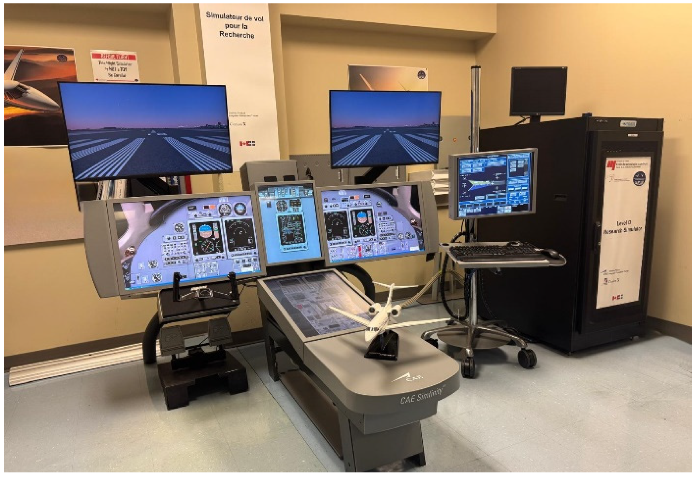
For the development and validation of the proposed autopilots, simulated flight data from a Research Aircraft Flight Simulator (RAFS) (Figure 1) with Level D flight dynamics have been gathered in order to model the Cessna Citation X flight dynamics. The RAFS is therefore a valuable platform for flight control studies due to its performance and realistic system data.

2.2. Cessna Citation X Simulink Platform

The Simulink platform of the Cessna Citation X was developed in earlier studies and validated against flight simulation data gathered from the RAFS [40]. The platform incorporates high-fidelity aerodynamic and engine models, nonlinear actuator dynamic models, and equations of motion that accurately represent the aircraft’s flight dynamics. It also integrates environmental modules, such as wind models, as well as failure scenarios involving engine failures or aerodynamic effects. These components were validated against RAFS flight-test data with less than 5% error [40]. The RAFS, manufactured by CAE Inc., Montreal, QC, Canada, is qualified to Level D for flight dynamics. According to the FAA, Level D is the highest qualification level for flight simulators, ensuring that simulation outputs closely match real-flight behaviour within certified tolerances. This certification supports the generalizability and practical relevance of the proposed control algorithms when evaluated in this environment.
Additionally, the Simulink model includes linearization capabilities at specified calibrated airspeeds (CASs) and altitudes, supporting a variety of control design approaches. This platform has been successfully used in prior work for designing controllers such as Linear Quadratic Regulators (LQRs) [36], fuzzy controllers [20], sliding mode controllers [41], hybrid adaptive controllers [42] and hybrid MPC controllers [13].

3. Design Methodology

3.1. Inner-Loop Controllers and Autopilot Design Requirements

The autopilot system for the Cessna Citation X is designed to satisfy key performance and safety requirements derived from certification standards. The CSAS and autopilots are designed to operate over an altitude range of 1500 ft (MSL) to 51,000 ft, covering the aircraft’s certified service ceiling and ensuring flight-envelope protection under all operating conditions. Throughout this altitude range, the system maintains the load factor within certified structural limits, thereby preserving airframe integrity and ensuring passenger comfort during cruise and flight-level changes. In addition, the CSAS complies with the Level 1 flying-qualities given in MIL-STD-1797A [43]. The design requirements are summarized in Table 2.

3.2. Adaptive Autopilot Architectures

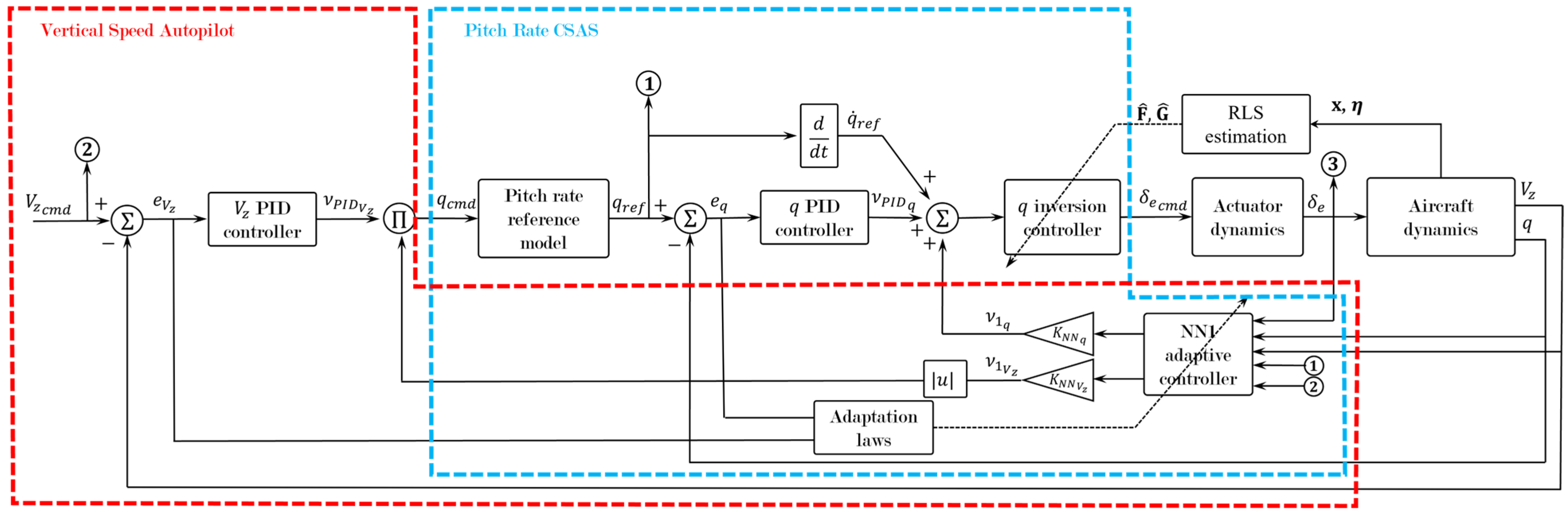
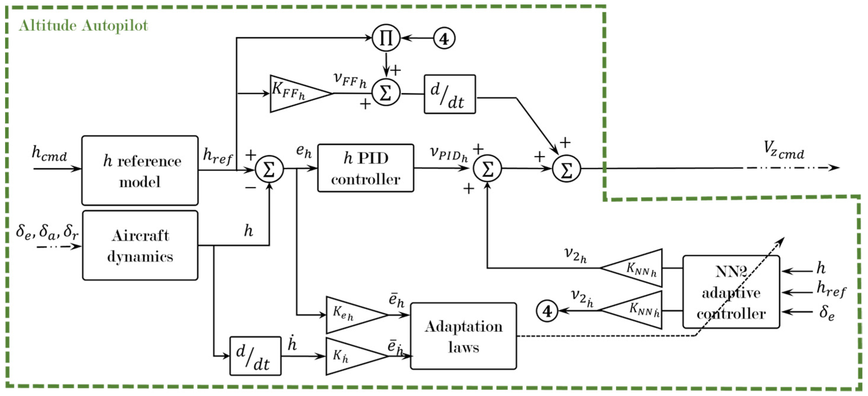
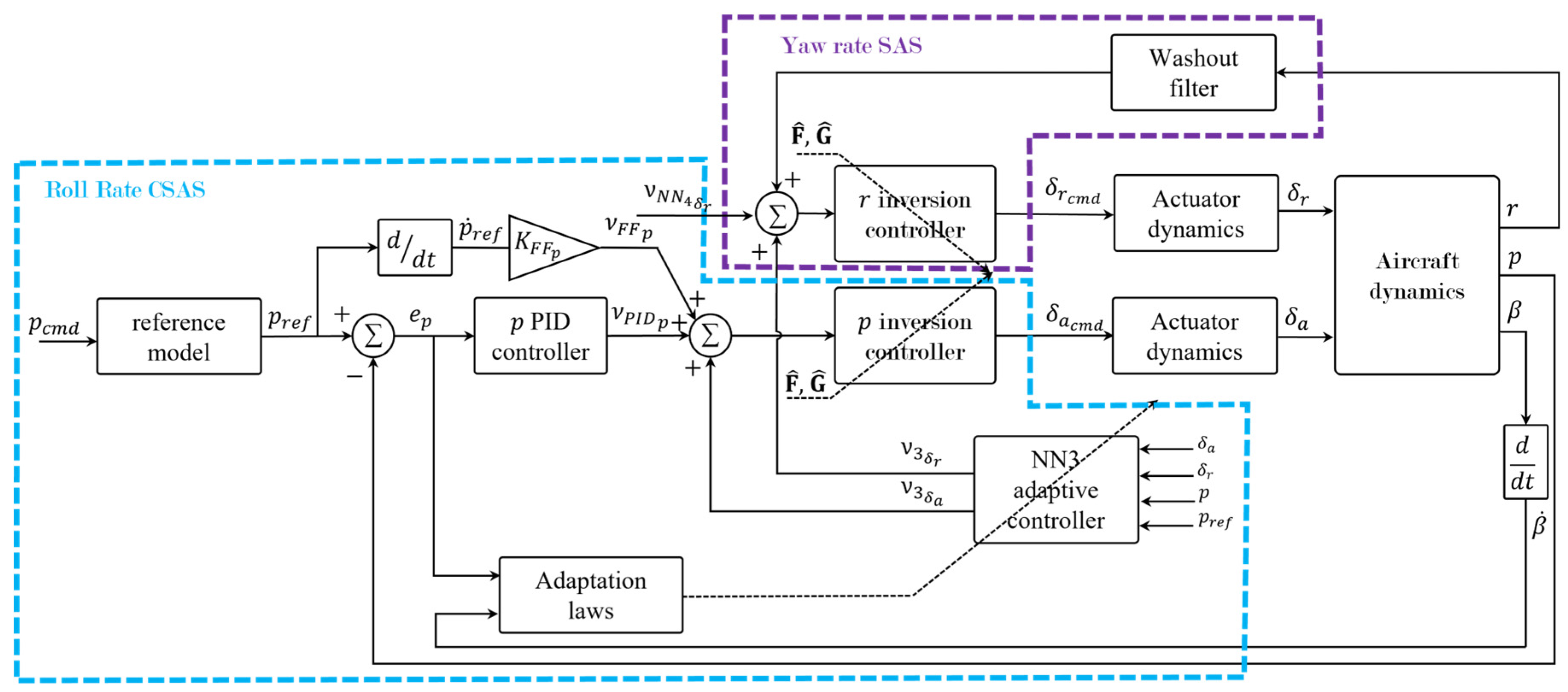
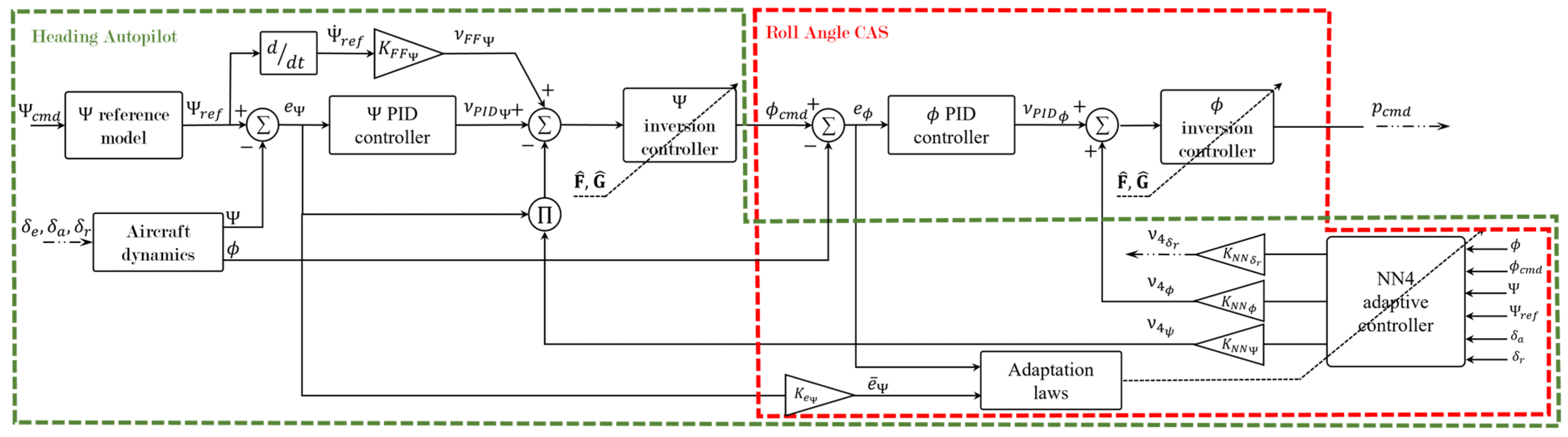
The complete controller and autopilot architectures are illustrated in Figure 2, Figure 3, Figure 4 and Figure 5. Figure 2 presents the inner-loop pitch rate controller and the outer-loop vertical-speed autopilot. Figure 3 illustrates the altitude autopilot. Figure 4 and Figure 5 detail the lateral control loops, including the roll rate and roll angle CSAS and the heading autopilot.

3.3. Aircraft Nonlinear Dynamics

This study considers longitudinal and lateral aircraft dynamics. The aircraft’s nonlinear dynamics can be expressed as
x ˙ = φ x , η y = ( x )
where the state vector x and the control input vector η are defined as follows:
x = x l o n   x l a t T η = δ e δ a δ r T
with
x l o n = u w q θ V z h T and   x l a t = v p r ϕ Ψ T
Here, x l o n is the longitudinal state vector, including the longitudinal and vertical velocity components u and w , the pitch rate q , the pitch angle θ , the vertical speed V z , and the altitude h . The lateral state vector x l a t includes the lateral velocity component v , the roll and yaw rates p and r , the roll angle ϕ , and the heading angle Ψ . The control input vector η includes the elevator δ e , aileron δ a , and rudder δ r angles. The functions φ and represent the (unknown) nonlinear dynamics and output mappings, respectively.
The nonlinear formulation in Equation (1) captures the full variations in the aircraft states and control inputs. Unlike conventional linear state-space models, it is well suited for the design of nonlinear controllers and autopilots.

3.4. Nonlinear Actuator Dynamics

The actuator models were implemented on the Simulink platform using second-order nonlinear transfer functions to capture the higher-order nonlinearities present in real actuator dynamics. The key parameters defining the actuator dynamics are given in Table 3.

3.5. Mathematical Foundations and Control Elements

This section presents the controller and autopilot designs, and reviews the inner-loop controllers, including the pitch and roll rate controllers, and the yaw rate stabilization. The control loops and command laws for the vertical speed, altitude, and heading autopilots are described separately in Figure 2, Figure 3, Figure 4 and Figure 5. The designed control system consists of multi-stage adaptive control loops that combine adaptive neural networks (NNs), Recursive Least Squares (RLS) dynamic inversion, and conventional linear PID controllers. Additional elements, such as feedforward filters, were incorporated to enhance transient response and overall performance.
Four neural networks, respectively labelled N N 1 , N N 2 , N N 3 and N N 4 , were developed and integrated, as shown in Figure 2, Figure 3, Figure 4 and Figure 5. The adaptive signals produced by the neural network controllers were denoted according to their corresponding inputs and outputs. For example, ν 4 δ r denotes the adaptive control signal generated by N N 4 for the rudder deflection δ r . Adaptive laws are used to update the neural network weights and the RLS parameters, ensuring convergence and stability. These laws have been derived to minimize tracking errors while guaranteeing the boundedness of the adaptive signals. Additional feedforward filters and disturbance rejection strategies were incorporated to enhance transient response and robustness in the presence of uncertainties.
These control elements and their mathematical foundations enable the design of robust adaptive autopilots capable of operating effectively across the cruise flight envelope of the CCX, while maintaining performance in the presence of uncertainties and nonlinearities such as turbulence and wind gusts.

3.5.1. Dynamic Inversion Controller

The CCX nonlinear dynamics can be written in affine form with respect to the control input as
x ˙ = f x + g x η
where f · and g · are nonlinear functions describing the aircraft dynamics. The measured output y i is expressed as
y i = C i x
The dynamic inversion controller aims to compute the control input η that will directly achieve a desired state derivative x ˙ , which can be written conceptually as an inverse mapping:
η = φ 1 ( x ˙   , x )
To obtain a local linear approximation, the aircraft dynamics are linearized about a nominal operating point ( x 0 , η 0 ). Using a first-order Taylor series expansion, the incremental dynamics Δ x ˙ can then be approximated locally as follows:
Δ x ˙ = F x 0 , η 0 Δ x + G x 0 , η 0 Δ η
where F x 0 , η 0 and G x 0 , η 0 are the Jacobian matrices evaluated at ( x 0 , η 0 ), defined by
F x 0 , η 0 = f x x + g x x   η x 0 , η 0 ;   G x 0 , η 0 = g x x 0 , η 0
Using the output relation in Equation (5) together with the linearized dynamics in Equation (7), the incremental control input Δ η required to track a reference signal r s can be computed using the following control law:
Δ η = C G x 0 , η 0 1     r ˙ s + ν   C F x 0 , η 0 Δ x
where C is the output matrix, and the signal ν is chosen to reduce the tracking error according to [3]:
e ˙ = ν
With an appropriate choice of ν , this formulation stabilizes the tracking error e , ensuring convergence and stable tracking of the desired reference signal.

3.5.2. Online State Estimation

The state variation at time step k + 1 , denoted by Δ x k + 1 , depends on the current state variation Δ x k and the control input variation Δ η k . Based on Equation (7), the state equation can be written as
Δ x ^ k + 1 = Δ x k Δ η k   F ^ k T G ^ k T
where F ^ k T and G ^ k T are the Jacobian matrix estimates.
Let us consider Θ ^ k   = F ^ k T G ^ k T as the vector of unknown parameters and X k = Δ x k Δ η k T as the vector of past increments. With these definitions, Equation (11) can be compactly rewritten as
Δ x ^ k + 1 = X k T Θ ^ k
where Θ ^ k can be estimated online using the Recursive Least Squares (RLS) algorithm.
The RLS prediction error ϵ k is defined as follows:
ϵ k = Δ x k   Δ x ^ k
where Δ x k is the measured state variation and Δ x ^ k is its estimated state variations.
Following the method described in [14], the parameter vector Θ ^ k can be updated using the following law:
Θ ^ k = Θ ^ k 1 + L k 1 X k κ + X k T L k 1 X k   ϵ k
where L k is the covariance matrix, which is numerically computed as follows:
L k = 1 κ     L k 1 L k 1 X k X k T L k 1 κ + X k T L k 1 X k  
Equations (14) and (15) are derived from the matrix inversion lemma, as detailed in [14]. Note that in this RLS formulation, F ^ k T and G ^ k T depend on the increment vector X k , rather than on the absolute state and control values.
Before running the algorithm, Θ 0 , L 0 , and κ must be initialized. In this work, in order to improve stability, the covariance matrix L k is updated conditionally: L k is reset when the prediction error ϵ k exceeds a prescribed threshold; i.e., ϵ k > ϵ t r e s h o l d . Here below in Table 4 is given a pseudo-code for the covariance matrix update.

3.5.3. NN Controller

Using the error estimates in Equation (13) often leads to non-negligible prediction errors in practical applications [44]. Therefore, the actual output variation at the time step k + 1 can be expressed in discrete form as
Δ y ^ k + 1 = Δ y k + 1 ε 1
where Δ y ^ k + 1 is the estimated output variation and ε 1 denotes the RLS estimation error.
Substituting this relation into the control law in Equation (9), the control input variation Δ η k can be rewritten as follows:
Δ η k = C G ^ k 1 [ r s ˙ + v   C F ^ k Δ x ε 1 ]
where C G ^ k and C F ^ k represent the locally estimated aircraft dynamics. An adaptive term is introduced to compensate for the RLS estimation error, such that
ε 1 = ν a d
A feedforward neural network (FFNN) is used to compute ν a d as an adaptive component.
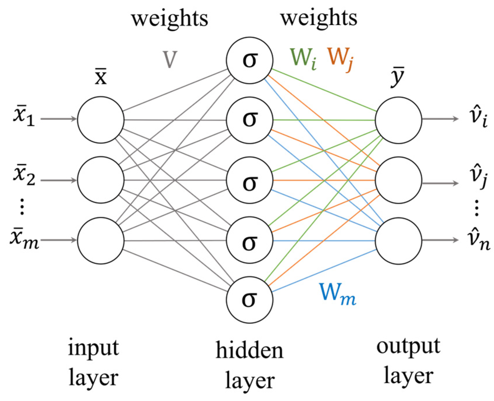
Figure 6 illustrates the architecture of the FFNN used in the CSAS and in the autopilots. The NN’s performance depends on the number of neurons, the number of hidden layers, the activation function, and the associated weight matrices.
The adaptive output signal of the neural network can be expressed as follows [3]:
ν ^ i = W i T σ V T x ¯
where the activation function σ R N × 1 is applied elementwise to the N neurons in the hidden layer. The input vector is defined as x ¯ = x ¯ 1 x ¯ 2 x ¯ m T . The weight matrices are W R N × n and V R m × N , where m and n denote the number of inputs and outputs, respectively. The activation function used in this work is the sigmoid function, defined as
σ i z = 1 1 + e z
A linear function is used for both the input and the output layers. As seen in Figure 2, Figure 3, Figure 4 and Figure 5, the neural network adaptive signals are scaled by a gain factor K N N i , which is used to adjust the amplitude of the adaptive correction term ν a d .

3.5.4. NN Adaptation Laws

The neural network weights are updated online using adaptation laws derived from the backpropagation algorithm [45,46,47]:
W ˙ i = σ σ   V T x ¯   e i T + λ   e i W i   Γ i V ˙ = Γ V [ x ¯ e i T W i T σ + λ   e i V ]
Here, e i is the tracking error vector corresponding to the i -th controlled variable, Γ i is the learning rate matrix for the i -th output of the NN, Γ V is the input layer learning rate, and σ is the gradient of the activation function σ . The scalar λ is set to 1.
The additional terms λ e i W i and λ e i V are defined to guarantee robustness and stability, as demonstrated through Lyapunov’s direct method. These update laws are based on the backpropagation theory [45,46,47].

3.5.5. PID Controllers

From the inversion control law, a linear feedback controller ν is required [3]. The feedback term ν is solely designed to ensure system stability. To model ν , a basic Proportional–Integral–Derivative (PID) controller is typically sufficient and can be expressed as follows [3]:
ν i   = K P + K I s + K D   s e i
where K P , K I and K D are the proportional, integral, and derivative gains, s is the Laplace operator, and i indexes the controlled variable.

3.6. Longitudinal and Lateral CSAS Inner Loops

In this research, the longitudinal and lateral Control Stability Augmentation System (CSAS) consists of low-level inner-loop controllers that ensure robust and stable tracking and are included within higher-level adaptive autopilots.
The longitudinal CSAS is designed to control the pitch rate q and to stabilize the short-period dynamics. It provides a fast feedback loop that improves pitch stability and reduces pilot workload. Building on this foundation, the longitudinal autopilot regulates vertical speed and altitude by commanding appropriate pitch rate responses, enabling smooth vertical flight path tracking even in the presence of disturbances.
Regarding the lateral dynamics, the CSAS focuses on controlling the roll rate p and stabilizing the yaw rate r by damping the Dutch-roll mode, which is essential for maintaining directional stability. The lateral autopilots then command the roll angle φ and heading Ψ , allowing coordinated control for accurate bank-angle regulation and heading tracking. A key contribution of this work is the integration of an adaptive Aileron–Rudder Interconnect (ARI) using neural networks, which improves yaw damping by adaptively coordinating aileron and rudder inputs.
These CSAS are model-reference controllers designed using prescribed reference signals. They have previously been validated for Level 1 flying qualities over the Cessna Citation X operational envelope [48]. Their proven performance provides a reliable foundation for the outer-loop adaptive autopilots developed in this study, ensuring stability and responsiveness during complex maneuvers even in the presence of uncertainties.

3.7. Pitch Rate CSAS

For pitch rate and roll rate control, a second-order transfer function is used as a reference model, which allows approximation of the short-period dynamics with specific frequency, damping ratio and time constant values, ω s p , ξ s p and T θ 2 , respectively. Their values have been set to satisfy Level 1 flight qualities according to MIL-STD-1797A [43]. Table 5 summarizes the mathematical design equations of the pitch rate controller.

3.8. Vertical-Speed Autopilot

The vertical-speed autopilot is designed to control V z . The designed autopilot uses a PID controller and an adaptive neural network N N 1 . Its primary control element equations are summarized in the following Table 6.

3.9. Altitude Autopilot

The adaptive neural network NN2 and a PID are used to track the desired altitude. The neural network receives the altitude error and its derivatives as inputs in the adaptation laws, enabling it to reduce tracking errors, stabilize altitude, and dampen oscillations during transient phases effectively. A ramp reference model is used to generate altitude commands. This model ensures smooth transitions between climb and cruise phases by shaping the altitude reference signal with a first-order transfer function. The ramp signal is designed to constrain climb and descent rates within 9.14 m/s [±1800 ft/min], thereby indirectly controlling the vertical speed and ensuring safe flight-level changes. The altitude autopilot design equations are summarized in the following Table 7.

3.10. Roll Rate CSAS and Yaw Rate Stabilization

The roll rate CSAS controller is designed using a Model-Reference Adaptive Control (MRAC) approach. A reference model is used to capture the desired roll and Dutch-roll dynamics based on flying quality specifications in MIL-STD-1797A [43], specifically the roll time constant τ r , damping ξ d r and natural frequency ω d r . The controller combines a conventional PID controller with dynamic inversion and adaptive neural network NN3. A feedforward term is included to anticipate changes in roll dynamics, while a washout filter is used to stabilize the yaw rate response during lateral maneuvers. Commands are generated for both the ailerons and rudder, accounting for actuator dynamics and coupling effects to ensure coordinated and stable lateral control.
In addition to stabilizing the yaw rate, the roll rate CSAS dampens the sideslip rate β ˙ , driving it toward 0. The sideslip rate β ˙ can be approximated by the following kinetic relationship [3]:
β ˙ v ˙ T A S
where v ˙ is the lateral acceleration and TAS is the true airspeed. Setting β ˙ to 0 allows fulfilling a coordinated turn with a dampened Dutch-roll effect. The roll rate CSAS design equations are summarized in the following Table 8.
K W F is the washout filter gain and τ is its time constant; C i is the output matrix with respect to the i -th variable state.

3.11. Roll Angle CSAS

The roll controller aims to regulate the aircraft’s roll angle ϕ in order to follow a command ϕ c m d . The control loop incorporates PID control, RLS dynamic inversion and adaptive neural network controller NN4. The roll controller design equations are summarized in the following Table 9.

3.12. Heading Autopilot

Finally, the heading autopilot is designed using equations described in Table 10. The autopilot uses a PID controller, RLS dynamic inversion and an adaptive neural network. A feedforward term is added to improve tracking of the heading reference signal. This formulation ensures precise and robust control of the aircraft’s heading by integrating model-based control with adaptive neural network compensation.

4. Results

This section presents the applications of the proposed CSAS and the adaptive autopilots. The simulations include nominal tests for parameter tuning as well as robustness evaluations under wind and turbulence. The evolution of the adaptive parameters is also shown, and system performance is assessed across the Cessna Citation X operating cruise flight envelope.
The simulation campaign is structured to progressively evaluate the controller performance, starting from nominal conditions, followed by robustness tests under disturbances, and finally validation across the complete cruise envelope. Each simulation case is designed to assess a specific aspect of controller performance, ensuring a comprehensive and logically connected evaluation framework.

4.1. Control Parameters

The control parameters presented in the previous equations were carefully tuned over the aircraft’s cruise flight envelope using parameter-sensitivity analysis, with their values summarized in Table 11 and Table 12.

4.2. Vertical-Speed Autopilot Tuning

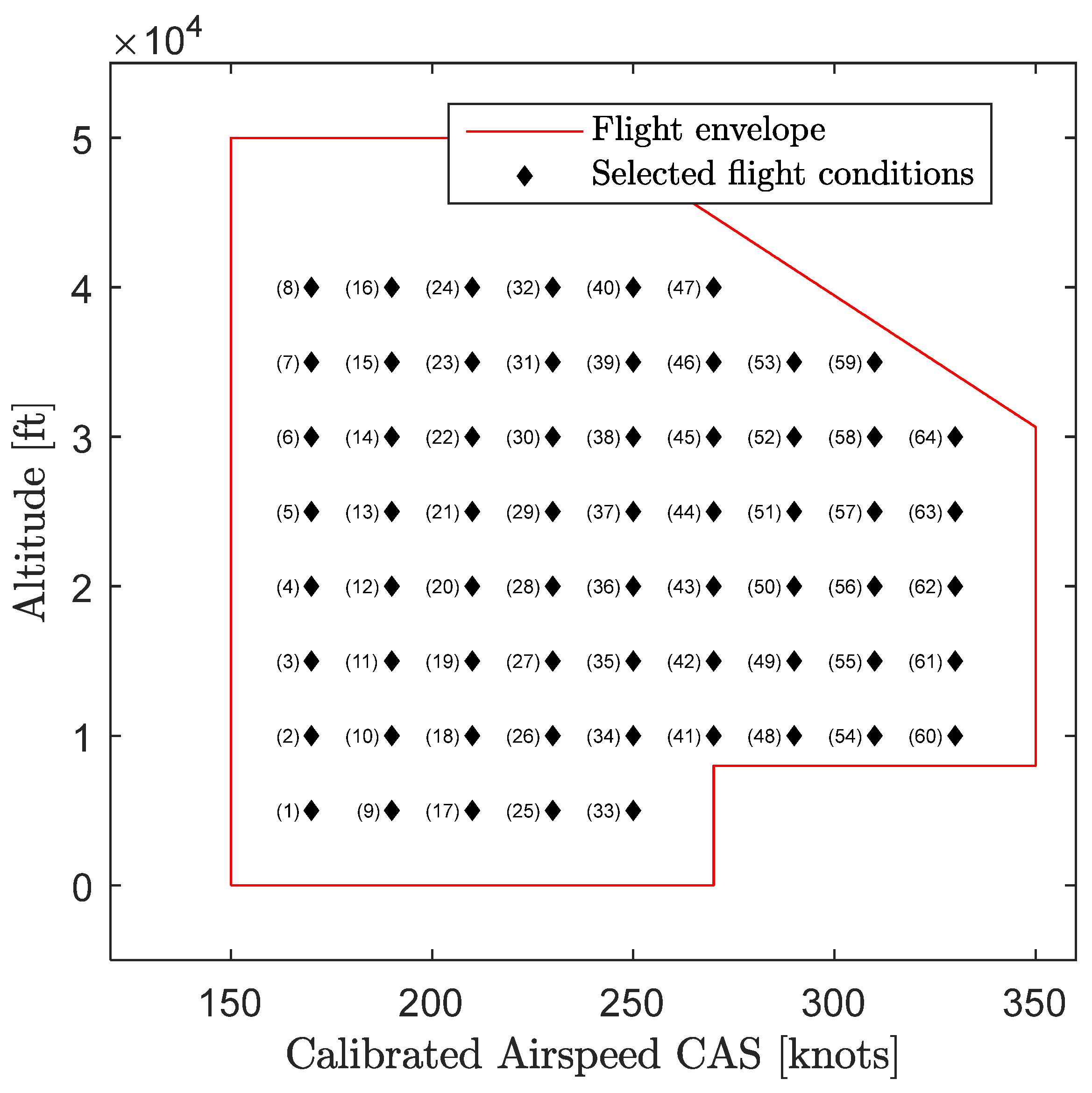
This section describes the tuning procedure for the vertical-speed autopilot. The tuning was carried out through a parameter-sensitivity analysis. The adaptive features were tuned using 64 representative cruise flight cases covering the Cessna Citation X cruise envelope.
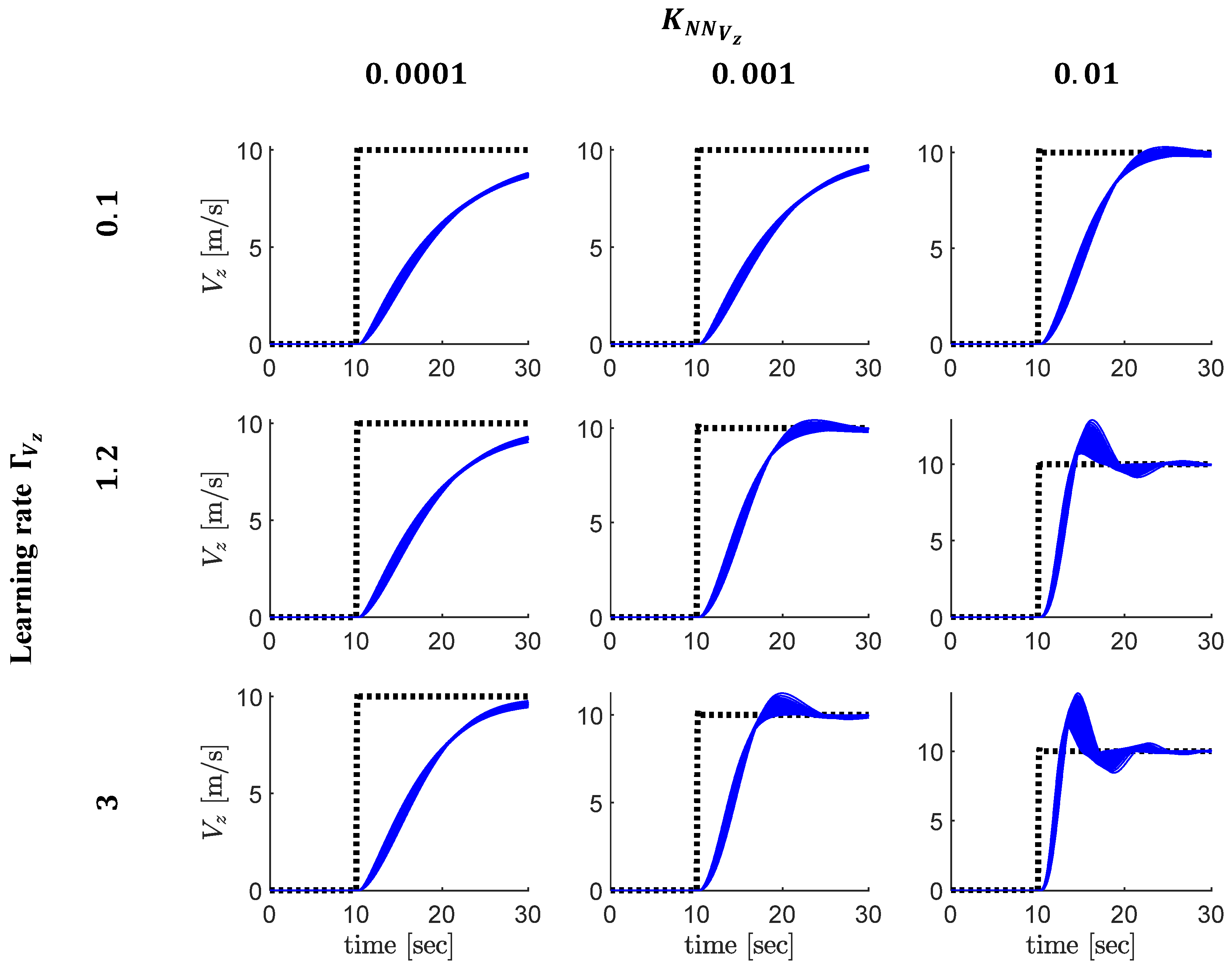
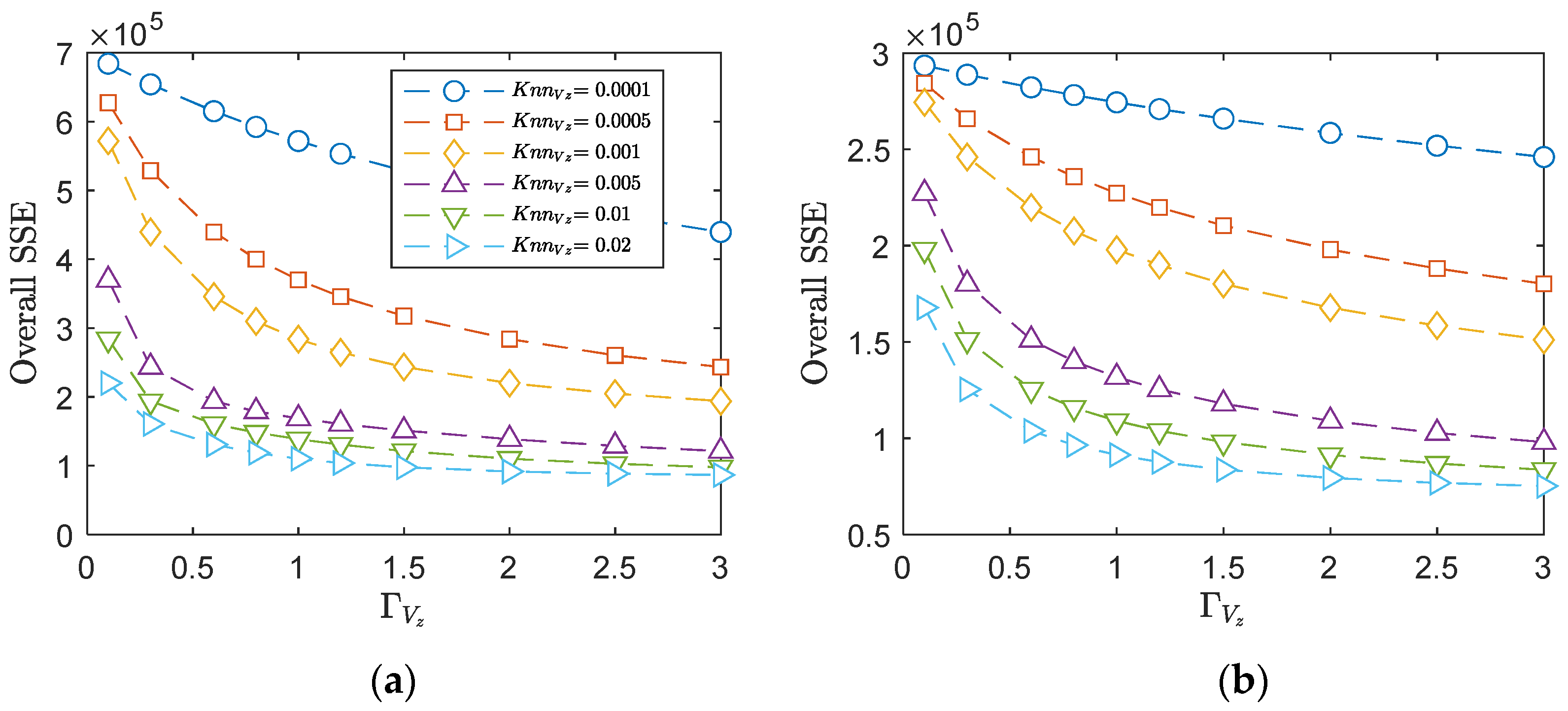
First, the PID controller was tuned. A single PID configuration was selected to ensure controller stability and convergence. The adaptive features were then tuned. For the vertical-speed autopilot, the neural networks’ learning rates Γ V z and gain K N N V z were set. Figure 7 shows the influence of these parameters on tracking performance. A suitable combination of parameters was found and is summarized in Table 11.
The NN learning rates and gains were optimized in the presence of uncertainties, as seen in Figure 8. In fact, incorporating uncertainties during the tuning process improves robustness and ensures reliable performance under off-nominal conditions. The optimization was performed by minimizing an objective function based on the overall Sum Squared Errors ( O v e r a l l   S S E ), defined as follows:
O v e r a l l   S S E = i = 1 i = N S S E i ;               S S E = Δ t t = 0 t = T V z c m d t V z t 2
where N is the number of simulated cruise scenarios.
The term S S E i is computed for each flight scenario, V z c m d and V z are the reference vertical speed and the vertical speed values at a given time step t , T is the simulation duration for a given flight condition, and Δ t = 0.02 s is the sample time. The remaining CSAS and autopilots, such as the altitude autopilot, roll controller and heading autopilot, were tuned following the same procedure. The parameters for each control algorithm are summarized in Table 11 and Table 12.

4.3. Altitude and Heading Command at 35,000 ft and 290 Knots

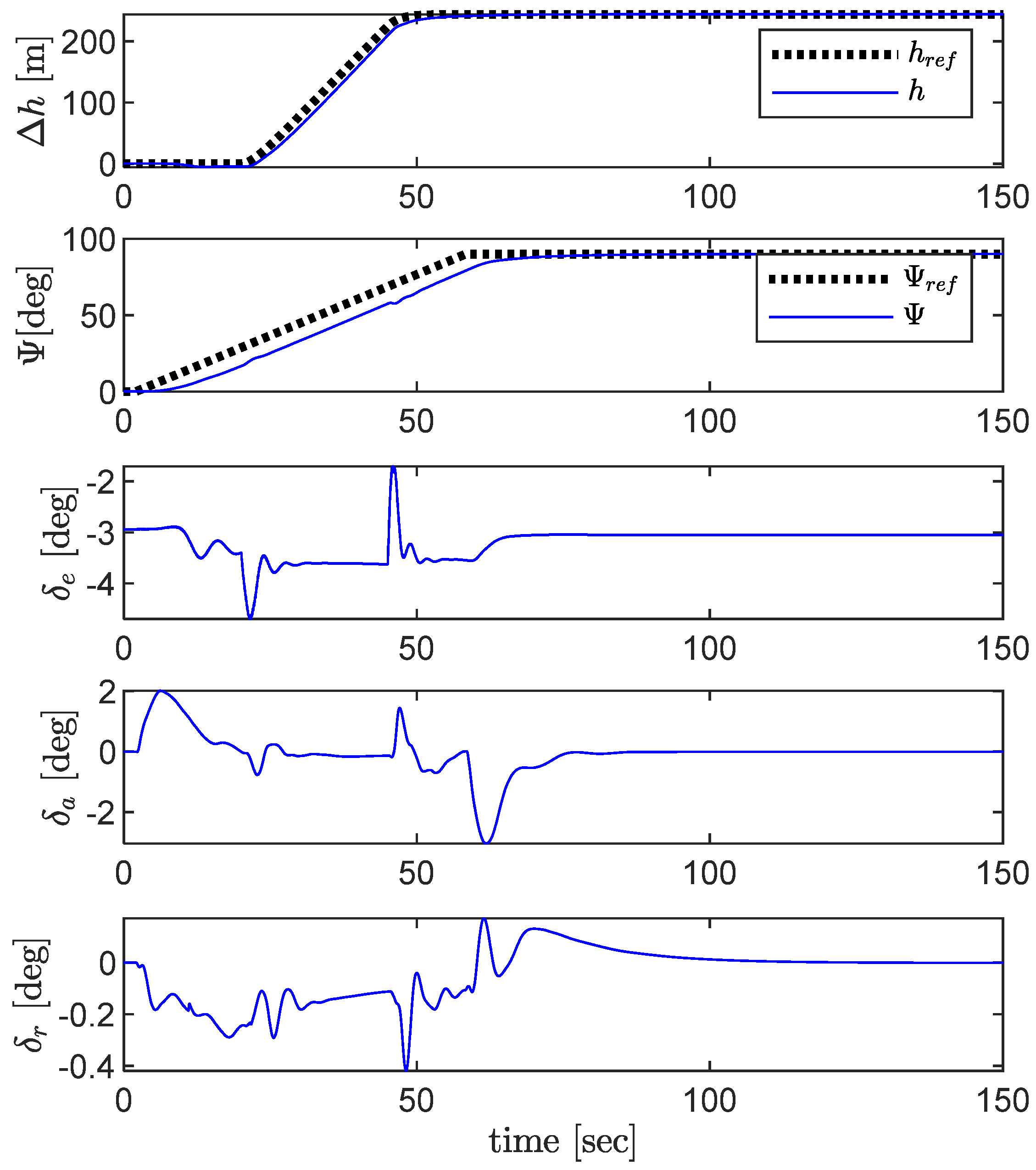
Once the CSAS and the autopilots were properly tuned, they were tested in flight simulation scenarios. First, a combined altitude and heading command was simulated under cruise conditions at an altitude of 10,600 m [35,000 ft] and a calibrated airspeed of 537 km/h [290 knots]. As seen in Figure 9, the altitude tracking consists of a flight-level change of 300 m [ 1000 ft], with a climb rate of 9.14 m/s [ 1800 ft/min], which effectively imposes an indirect vertical-speed command. Upon reaching the target altitude, the altitude capture mode engages automatically to ensure a smooth transition with minimal overshoot.
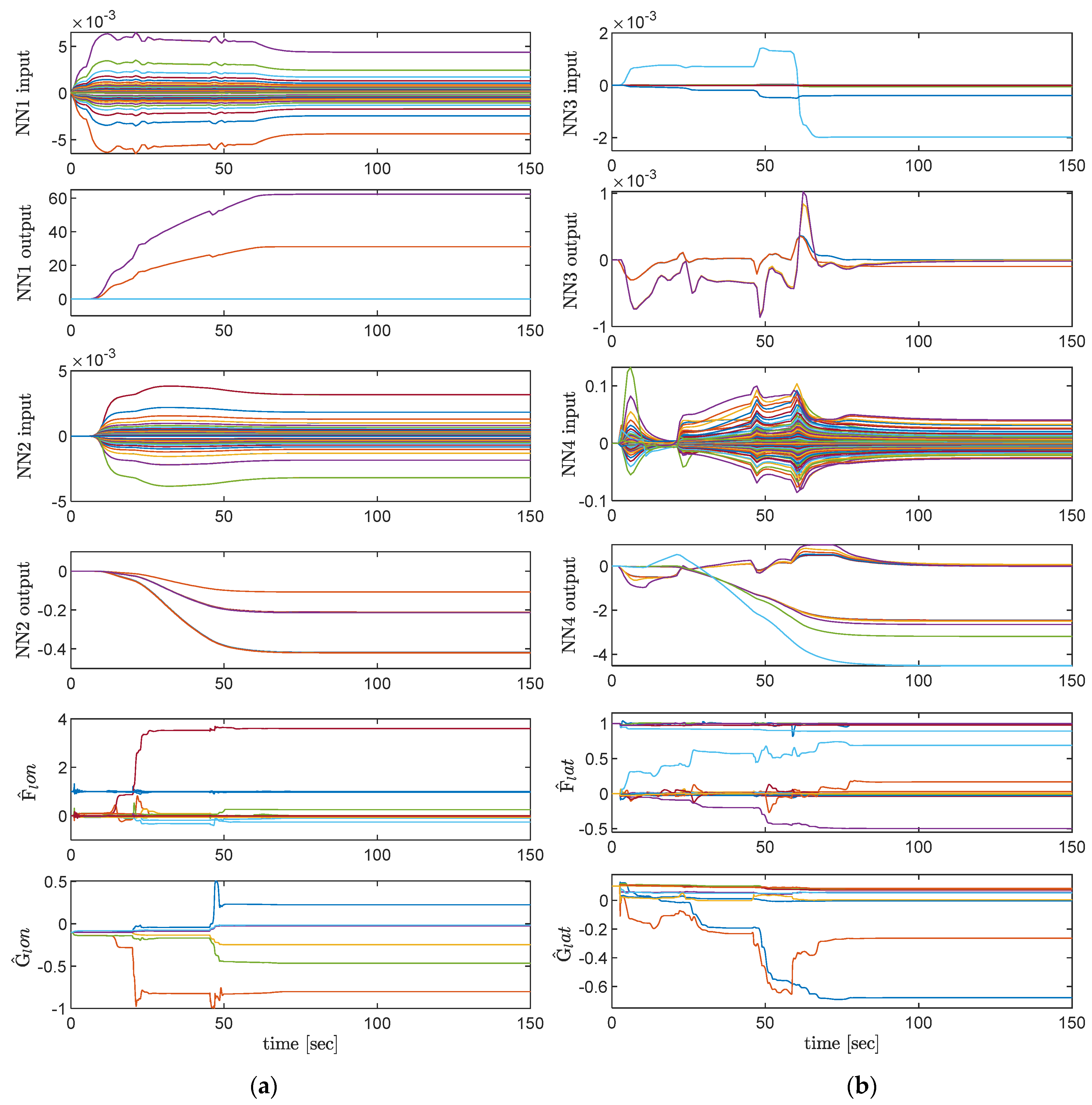
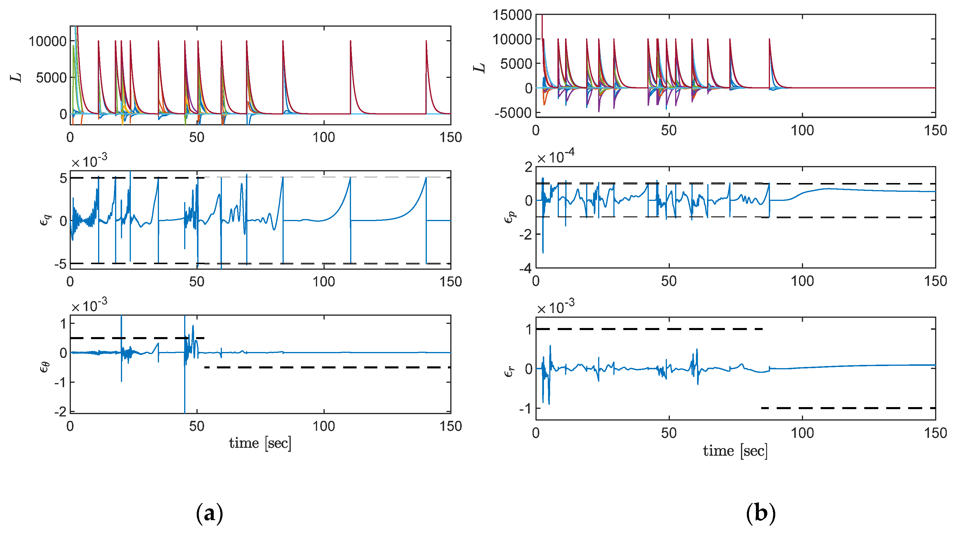
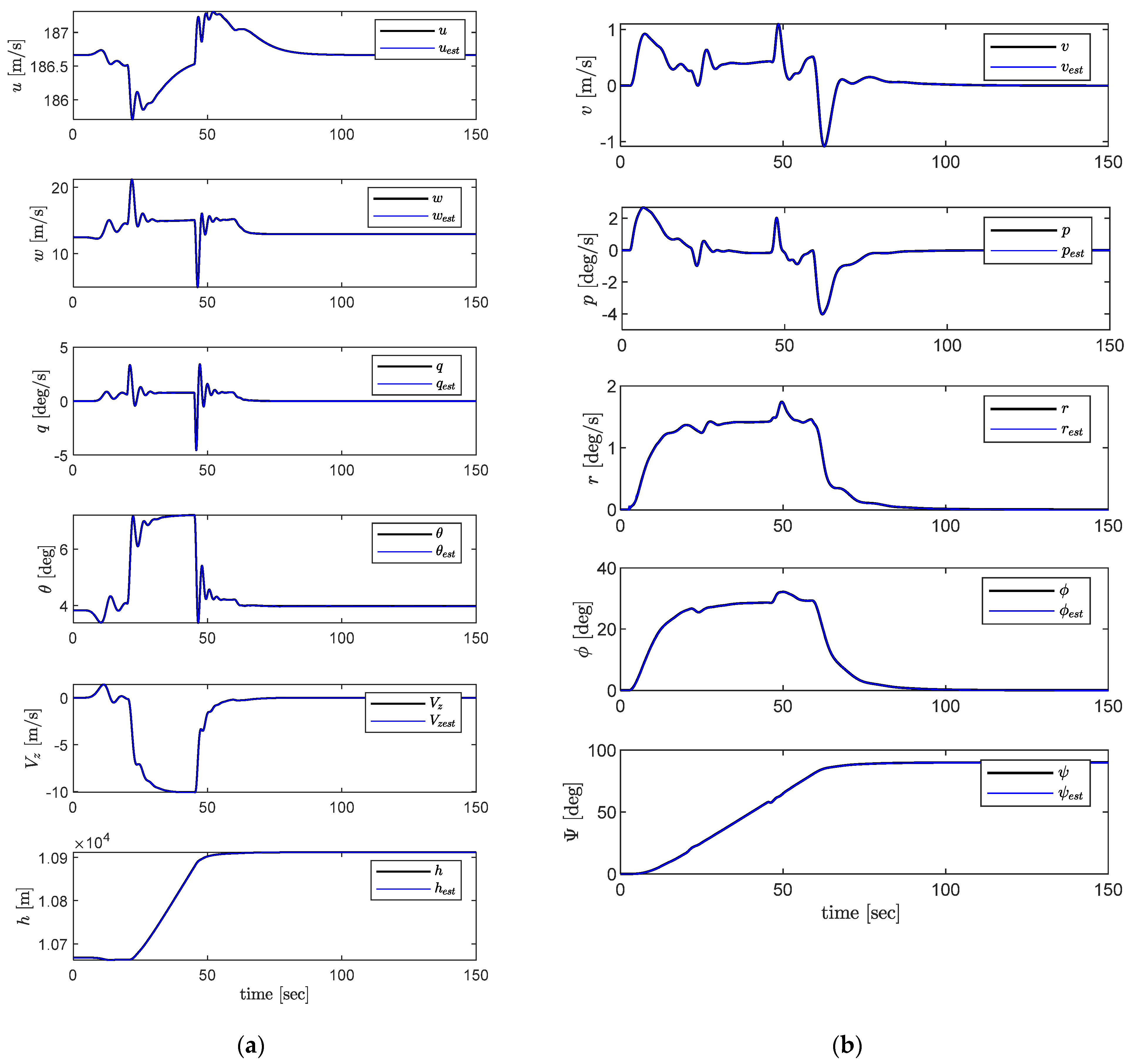
Simultaneously, a heading command of 90° is executed, allowing a coordinated turn with a constant turn rate of 3 ° /sec. This scenario is used to assess controller performance and coordination between the longitudinal and lateral control loops. Figure 10 and Figure 11 show the controller’s overall adaptive parameter variations, including the RLS estimation F ^ and G ^ , the covariance matrices L k , the estimation errors ϵ i , and the NN input and output weights V and W , while Figure 12 shows the resulting state estimations.
The RLS parameters’ numerical values are given below in Equation (32), showing their orders and dimensions for both longitudinal and lateral controllers. The values were registered at simulation time t = 15 s. F ^ l o n is a 6 × 6 state matrix, corresponding to six longitudinal states included in the state vector x l o n ; G ^ l o n is a 6 × 1 control matrix, corresponding to the elevator control input δ e , and the covariance matrix is a 7 × 7 matrix, corresponding to the sum of states and control inputs. The same logic applies to the lateral parameters F ^ l a t , G ^ l a t and L l a t , where the number of lateral states is five, and the control inputs are the ailerons δ a and the rudders δ r . As we can see from Equation (32), the state matrix F ^ l o n and F ^ l a t are close to the identity matrix, which is the right state-space representation in discrete time, thus showing that the RLS estimation is performed correctly. Also, the diagonal values of the covariance matrices x L l o n  and L l a t are high and positive, showing the positive definiteness of the matrices during estimation. Example values of the NN weights are not given here, as their dimensions are quite big and reach 7 × 30, depending on the number of neural network inputs and outputs and the number of neurons.
F ^ l o n = 0.985   0.0049   0.006   0.0054   0.0015   0.0013   0.245     1.04     0.0973     0.0924     0.0108     0.0107   0.0006   0.0003     0.999   0.0011     0     0   0.0002   0.0002   0.0012     0.999     0.0001     0   0.0312   0.0197     0.0893     0.0926     1   0.0038   0.0178     0.0002   0.0534   0.0559   0.0181     1   G ^ l o n = 0.0974   0.139   0.101   0.0994   0.138   0.0818   L l o n = 225   7.57   44.1   11.8   22.6   2.86     16.8   7.57     0.557   12.1   6.35   0.570     0.0019     5.46   44.1   12.1     963   0.736   4.08   2.13     1.01   11.8   6.35   0.736     965     5.42   0.807     0.322   22.6   0.57   4.08     5.42     2.47     0.364   0.0424   2.86     0.0019   2.13   0.807     0.364     0.0745     0.333   16.8     5.46     1.01     0.322   0.0424     0.333     965   F ^ l a t = 0.977   0.241   0.0595     0.07   0.123   0.0018     0.97   0.0103     0.0062   0.0065   0.0029   0.0232     0.924     0.0138   0.0122   0.0013     0.0002   0.0184     1.01   0.009   0.0015   0.0187   0.0195     0.0105     0.989   G ^ l a t = 0.0181   0.188   0.0996     0.0559   0.110     0.0542   0.103     0.0211   0.105     0.0132   L l a t = 10.3   42.7   4.99   25.3     35.5   3.22   29.4   42.7     527   4.78     58.2   47.2   8.99   27.3   4.99   4.78     580   16.7   22.1   0.988   2.49   25.3     58.2   16.7     77.9   118     18.5     39.7   35.5   47.2   22.1   118     190   20   22.5   3.22   8.99   0.988     18.5   20     579   5.51   29.4   27.3   2.49     39.7   22.5   5.51     565  

4.4. Validation for the Cessna Citation X Cruise Flight Envelope

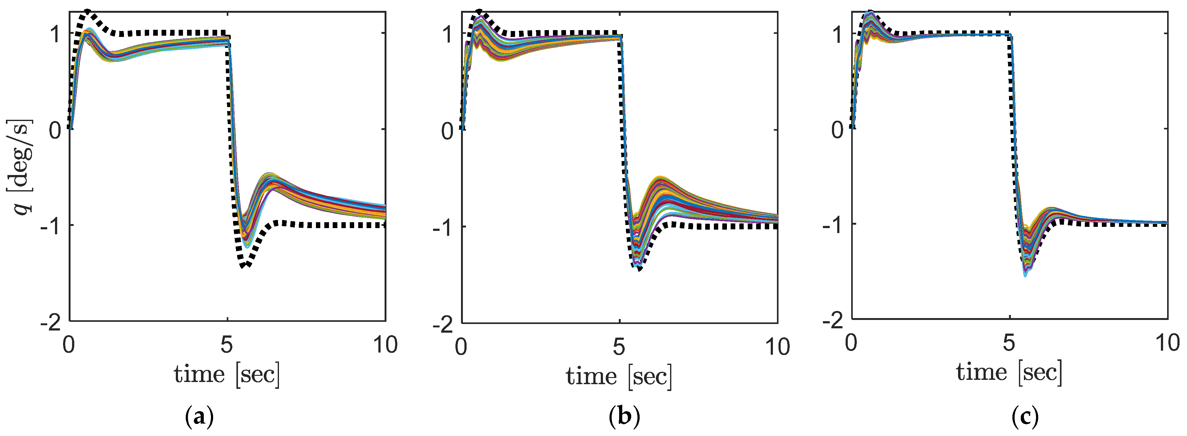
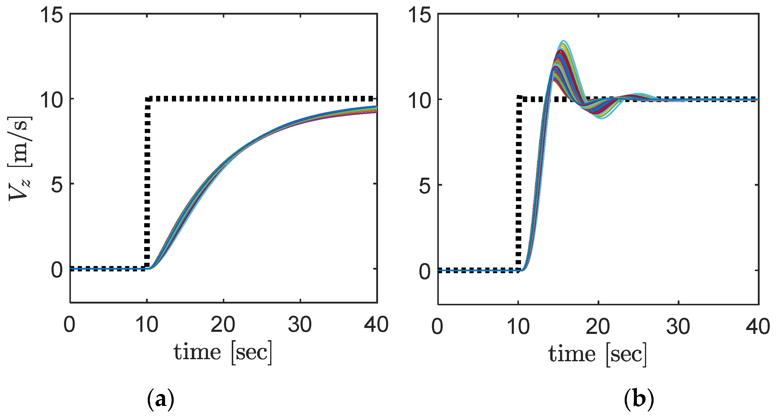
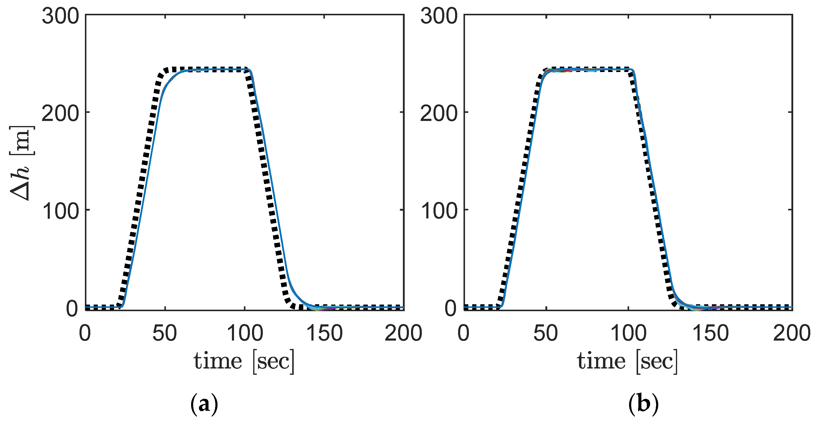
The CSAS and the autopilots were tested across the Cessna Citation X cruise operational envelope. The cruise flight envelope was discretized into a set of flight points (trim conditions). As seen in Figure 13, a total of 64 representative cruise flight conditions were defined for altitudes ranging from 5000 ft to 40,000 ft, while the calibrated airspeed was varied from 170 to 330 knots. Each CSAS and autopilot was tested, with and without their adaptive elements, as seen in Figure 14, Figure 15, Figure 16, Figure 17, Figure 18 and Figure 19. Overall, the controllers with adaptive elements exhibit improved tracking performance, following the reference commands more closely than their non-adaptive counterparts.

4.5. Performance Results

The CSAS and autopilot performances are summarized in the following Table 13. The inner-loop CSAS, including the pitch rate and roll rate responses, presents damping and frequency characteristics, as they are oscillatory motions related to the short-period and Dutch-roll dynamics. Comparing the results with the flight quality specifications provided by [43], we can conclude the inner-loop controllers respect the Level 1 flight quality criteria and are therefore suitable to implement within the trajectory tracking controller. The vertical speed overshoots by between 11% and 34%, depending on the flight conditions; however, the settling and rising times are short enough for longitudinal maneuvers. Also, the altitude and the heading autopilots present negligible overshoots and short enough settling times, which are the requirement for smooth flight-level changes and coordinated turns, thus ensuring passenger comfort.

5. Robustness Tests

5.1. Wind and Turbulence Tests

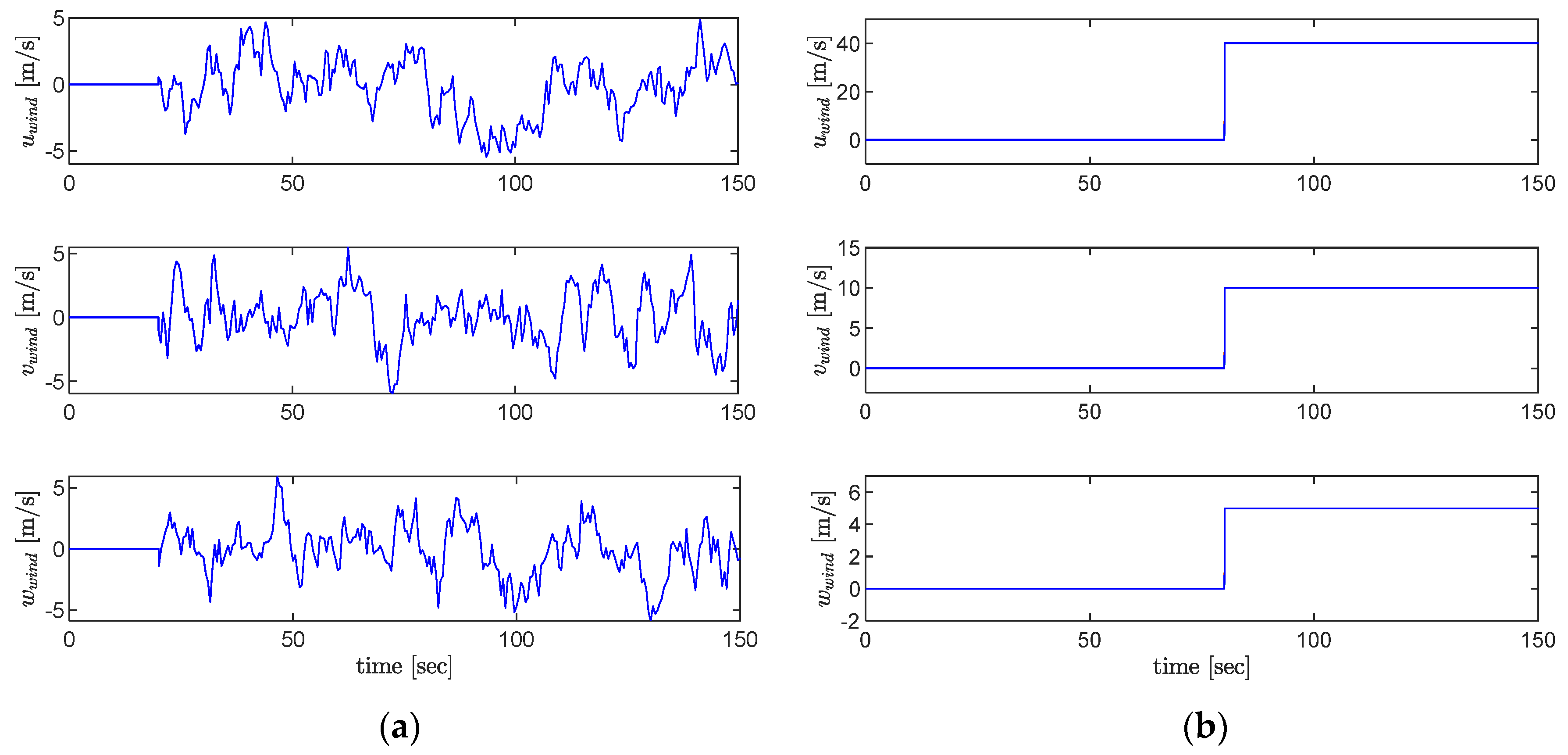
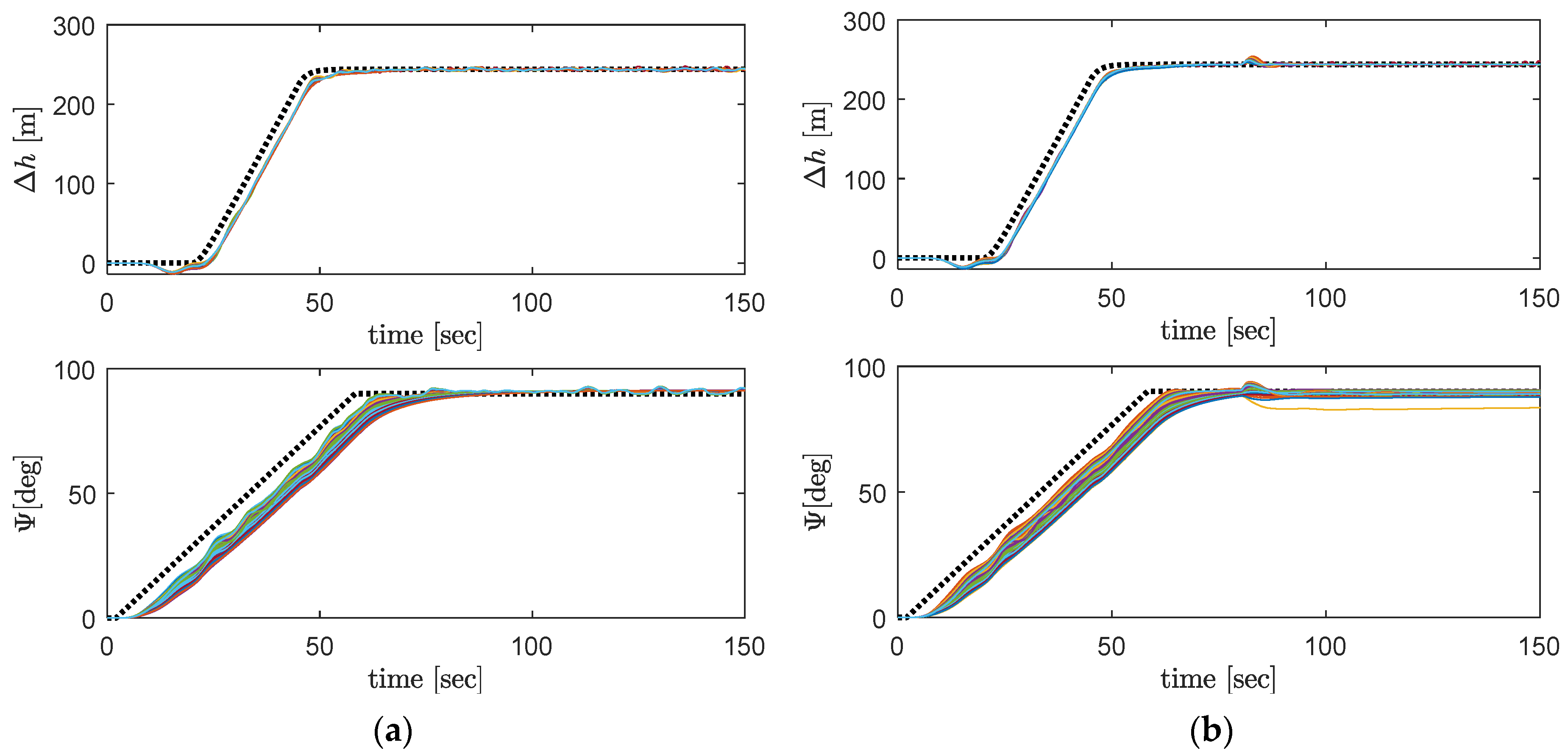
The CSAS and the autopilots were tested in the presence of external disturbances such as wind gusts and turbulence. The disturbances were simulated using a Dryden turbulence model, and they were directly implemented on the aircraft model dynamics. Figure 20 illustrates the wind and turbulence profiles, while Figure 21 shows the coordinated altitude and heading tracking for 64 representative cruise conditions.

5.2. Flight Simulation Comparison in the RAFS

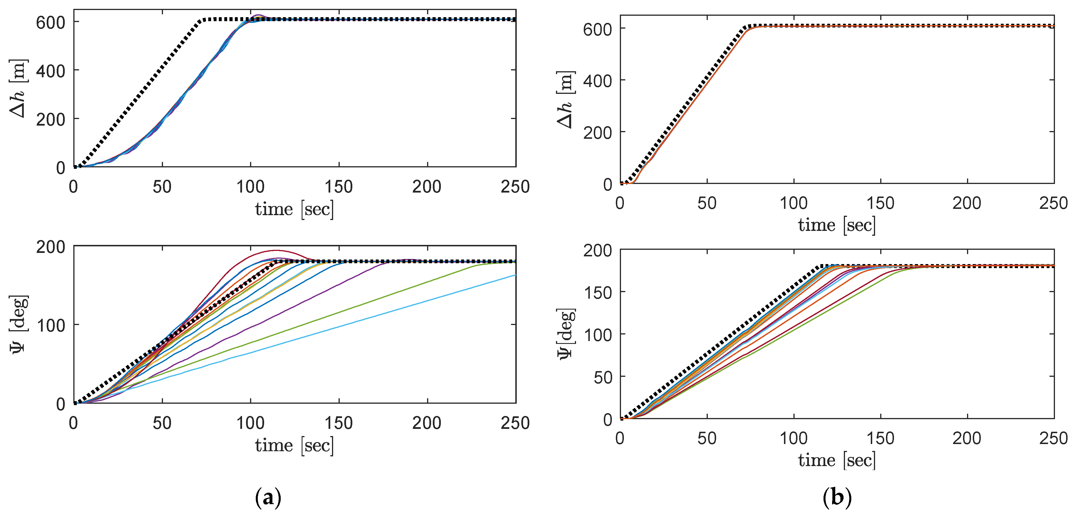
Finally, the altitude and heading autopilots were compared with those of the real Cessna Citation X using flight simulations in the Research Aircraft Flight Simulator (RAFS), and the comparison results are given in Figure 22. Saturators were added according to the aircraft performance limitations as specified in Table 2.

6. Discussion of Results

6.1. CSAS and Autopilot Architectures

The CSAS and autopilots developed for the Cessna Citation X contained three inner-loop controllers for the pitch rate, roll rate, and roll angle control, and three outer-loop autopilots for the vertical speed, altitude, and heading command. Their respective architectures are illustrated in Figure 2, Figure 3, Figure 4 and Figure 5, where Figure 2 shows the pitch rate and vertical-speed autopilot configuration, Figure 3 shows the altitude autopilot, and Figure 4 and Figure 5 show the complete set of autopilot architectures, including the heading autopilot with the roll angle control and yaw rate stabilization. The CSAS design objectives were established to satisfy MIL-STD-1797A Level 1 flight quality criteria across the CCX cruise flight envelope [43]. The longitudinal system architecture included the pitch rate, vertical speed, and altitude autopilots, whereas the lateral directional system architecture integrated roll rate, roll angle, and heading control with yaw rate stabilization. In addition, the yaw stabilization was fulfilled through dampening of the sideslip angle derivative.
The CSAS and hybrid adaptive architectures combined PID control for baseline stability, Recursive Least Squares (RLS)-based dynamic inversion, and neural network (NN) adaptation for residual error compensation. Dynamic inversion (DI) was applied to the CSAS controllers and heading autopilots, while the altitude and vertical-speed autopilots used PID–NN configurations. DI was not applied to the altitude and vertical-speed command due to small value inversion, which may lead to zero division and, thus, numerical instabilities when inverting the control matrices G V z and G h .

6.2. Tuning and Adaptation

In sum, the controllers and autopilots overall were tuned and validated for 64 representative cruise flight conditions with varying altitudes from 1500 m [5000 ft] to 12,200 m [40,000 ft] and calibrated airspeeds between 314 km/h [170 knots] and 611 km/h [330 knots], as shown in Figure 13. Parameter tuning was fulfilled using sensitivity analysis and global optimization, as shown in Figure 7 and Figure 8, to identify a single robust controller configuration. The RLS estimator provided accurate local linearization, with updates triggered only when the estimation error exceeded a predefined threshold to avoid divergence, as indicated in Figure 11. The influence of the forgetting factor κ was analyzed; small κ values yielded faster but noisier updates, while higher κ values improved stability. The convergence of RLS estimated states, covariance matrices, and hyperparameters is shown in Figure 11, Figure 12 and Figure 13, confirming reliable estimation of both longitudinal and lateral dynamics. The neural network compensates for modelling errors from the RLS estimations. The normalization coefficient K e i was applied to the NN i t h input to keep error magnitudes near zero and stabilize weight adaptation, as depicted in Figure 14. The NN demonstrated effective learning for both single-loop and coupled-loop configurations, thus accelerating transient responses and reducing steady-state tracking errors.
Regarding numerical singularities associated with nonlinear dynamic inversion, they may arise when the control effectiveness matrix becomes ill-conditioned. In fact, as seen in the numerical values of G ^ l o n and G ^ l a t from Equation (32), their values can be very small and cross zero, as they constantly change through time. In the proposed adaptive autopilot architecture, this issue is mitigated by operating around trimmed flight conditions, and a covariance matrix update is performed. The inversion process is therefore performed on matrices whose determinants remain sufficiently far from zero, ensuring numerical stability and reliable control allocation. Furthermore, the adaptive neural network compensation and feedback control loops contribute to maintaining bounded system responses, which prevents the controller from driving the system toward singular configurations during the evaluated cruise flight conditions.

6.3. CSAS and Autopilot Performance

Three controller configurations were assessed: PID, PID–DI, and the full hybrid PID–DI–NN. As shown in Figure 14, Figure 15, Figure 16, Figure 17, Figure 18 and Figure 19, the hybrid adaptive design consistently achieved the best tracking and disturbance rejection performance. Pitch rate and roll rate controllers reached a steady state within 1.9 s with errors below 0.1%, meeting Level 1 flight quality by closely following reference signals. For vertical speed control, response times ranged from 5 s to 8 s, and settling times from 10 s to 15 s, while NN adaptation reduced transient response time by about 30%. The altitude autopilot achieved smooth altitude capture with minimal overshoot, improved by derivative-based NN weight updates near the target altitude. Roll control performance improved, notably by the use of dynamic inversion, and the addition of NN further decreased the settling time from 12 to 15 s to 8–10 s and eliminated residual steady-state errors. The heading autopilot accurately tracked a 3°/s standard turn rate, maintaining altitude–heading maneuver coordination. The combined altitude–heading maneuver at 35,000 ft and 290 knots is illustrated in Figure 21, and it confirms the controller’s ability to coordinate longitudinal and lateral control.

6.4. Robustness Validation

Robustness testing under Dryden turbulence and wind-gust disturbances, as shown in Figure 21, has validated the system’s resilience to uncertainties. Controller stability was preserved across all conditions without retuning or reconfiguration, and control-surface deflections remained within their physical required limits. Furthermore, the adaptive control elements demonstrated numerical stability and convergence. Thus, the adaptive autopilots maintained stable dynamics even when reference models were changed, confirming structural robustness.
Finally, a comparative validation using the Level D Research Aircraft Flight Simulator is shown in Figure 22. The proposed controller achieved faster and smoother trajectory tracking than the actual baseline Cessna Citation X autopilot. Despite minor actuator saturation limits in real flight, the adaptive-controller responses were nearly identical, demonstrating the realism and generalizability of the simulation results.

6.5. Stability Assessment

The stability and convergence of the proposed adaptive control architecture follow the Lyapunov-based framework commonly used in adaptive neural network control. According to the Lyapunov stability criterion, a positive definite candidate function L is selected such that L 0 and its time derivative satisfies L ˙ 0 , which guarantees boundedness of the closed-loop signals and convergence of the tracking error [49]. Neural network adaptive control laws derived using Lyapunov stability theory have been extensively established in the literature, where the weight adaptation laws are designed to ensure the negative semi-definiteness of the Lyapunov derivative and the boundedness of the neural network approximation error [45,50,51]. In addition, the parameter estimation used in the proposed controller relies on the Recursive Least Squares (RLS) algorithm, whose convergence properties and boundedness of the estimation error are well established in estimation theory [14]. Under appropriate excitation conditions, the RLS estimator ensures convergence of the estimated parameters and bounded estimation errors. Consequently, in this work, we assume that the combination of Lyapunov-based neural network adaptation and RLS parameter estimation guarantees bounded closed-loop signals and convergence of the tracking error for the proposed adaptive control system.

6.6. General Remarks

In sum, the designed controller’s main advantage is that it does not require any prior knowledge of the aircraft’s mathematical model. Control inputs are solely generated from online RLS estimated local dynamics, allowing dual adaptation using dynamic inversion and NN to maintain high controller accuracy and robustness throughout the cruise flight envelope. By combining the proven reliability of classical PID control with modern adaptive estimation and learning, the proposed architecture achieved stable, certifiable, and high-performance flight path control suitable for advanced business jet autopilot systems.

6.7. Future Works

Although the proposed adaptive autopilot architecture has been validated across 64 representative cruise flight conditions and evaluated under wind-gust and Dryden turbulence disturbances, further robustness assessment could be conducted using Monte Carlo simulations. Such an approach would allow a systematic statistical analysis of controller performance under randomized variations in aerodynamic parameters, actuator dynamics, sensor uncertainties, and environmental disturbances. In addition, the present work focuses primarily on cruise flight conditions. Future research will extend the proposed control framework to other flight regimes, including climb, descent, takeoff, and landing phases, where aircraft dynamics and operational constraints differ significantly. Investigating controller performance across the full flight envelope would further demonstrate the applicability of the adaptive architecture to complete flight missions. Finally, future developments may explore the integration of fault-tolerant control strategies to enhance system resilience in the presence of actuator or sensor failures. The inclusion of additional secondary control surfaces, such as spoilers, could also be investigated to improve control allocation and overall aircraft maneuverability.

7. Conclusions

7.1. Research Summary

This research mainly aims to:
  • Address Loss of Control In-Flight risks through enhanced flight control robustness.
  • Reduce the strong dependence of conventional controllers on gain scheduling and linear models.
  • Improve adaptability across the cruise flight envelope, while maintaining Level 1 flight quality requirements.
  • Bridge the gap between advanced adaptive control methods and practical implementation constraints, including flight quality requirements.
The key contributions can be enumerated as follows:
  • Designing hybrid adaptive controllers and autopilots combining PID, RLS-based dynamic inversion and neural network controllers.
  • Eliminating gain scheduling by enabling a single controller configuration that is valid across the cruise flight envelope.
  • Validating the designed controllers and autopilots throughout the cruise envelope of the Cessna Citation X by using a high-fidelity nonlinear flight dynamic model.
  • Comparing the adaptive autopilots with the actual autopilots mounted on the Cessna Citation X.

7.2. Conclusions

From the simulation results, the following conclusions can be formulated:
  • The hybrid adaptive controller and autopilots were successfully developed for Cessna Citation X flight dynamics. The proposed system included inner-loop CSAS controllers for pitch rate, roll rate, and yaw rate stabilization, and outer-loop autopilots for vertical speed, altitude, and heading control.
  • The controller achieves MIL-STD-1797A Level 1 flight quality across 64 cruise conditions using a single configuration without gain scheduling.
  • The RLS estimator and NN adaptation enable accurate online modelling and compensation of uncertainties, ensuring robust performance in the presence of wind gusts and turbulence.
  • The proposed controller outperforms baseline PID and PID–RLS designs, providing faster response, improved tracking accuracy, and effective disturbance rejection.
  • Validation with high-fidelity RAFS data confirms the practical feasibility, robustness, and real-world applicability of the approach.

Author Contributions

Conceptualization, R.P.A.; Methodology, R.P.A., H.R., L.P. and D.M.C.; Software, R.P.A., H.R. and D.M.C.; Validation, R.P.A., G.G., H.R., L.P. and D.M.C.; Formal analysis, R.P.A.; Investigation, R.P.A., R.M.B., H.R., L.P. and D.M.C.; Resources, G.G. and R.M.B.; Data curation, R.P.A.; Writing—original draft, R.P.A.; Writing—review & editing, R.P.A., G.G. and R.M.B.; Supervision, G.G. and R.M.B.; Project administration, G.G. and R.M.B.; Funding acquisition, G.G. and R.M.B. All authors have read and agreed to the published version of the manuscript.

Funding

This research was funded by the Canada Research Chair of Aircraft Modelling and New Simulation Technologies, grant number: 231679, and the NSERC CREATE UTILI program which helped in the realization and publication of this article. Ruxandra Botez is the Canada Research Chair Tier 1 Holder in Aircraft Modeling and New Simulation Technologies.

Data Availability Statement

The original contributions presented in this study are included in the article. Further inquiries can be directed to the corresponding author.

Acknowledgments

This study was carried out in the Laboratory of Applied Research in Active Controls, Avionics and AeroServoElasticity (LARCASE). Ruxandra Botez received the Cessna Citation X Research Flight Simulator (RAFS) through research grants authorized by the Canadian Foundation of Innovation (CFI), the Ministère du Développement Économique, de l’Innovation et de l’Exportation (MDEIE), and CAE Inc.

Conflicts of Interest

The authors declare no conflicts of interest.

Nomenclature

CoG ,   x c g centre of gravity, coordinate of the centre of gravity
f, gunknown nonlinear functions
h altitude
F , F ^ online state matrix and its estimate
G , G ^ online control matrix and its estimate
L covariance matrix
V , W neural network weight matrices
I N × N unit   matrix   of   size   N × N
K i gain   coefficient   corresponding   to   the   i -th signal
T θ 2 short-period time constant
V z vertical speed
x , x l o n , x l a t full state, longitudinal state and lateral state vectors
x ¯ NN input vector
m mass
p , q , r roll, pitch, and yaw rates
u , v , w longitudinal, lateral, and vertical velocity components
Γ i learning   rate   matrix   corresponding   to   output   i
δ e , δ a , δ r elevator, aileron and rudder deflections
ξ d r , ω d r Dutch-roll damping and frequency
ξ s p , ω s p short-period damping and frequency
ϵ i , RLS   approximation   error ,   respectively ,   to   i -th state
Δ t time step
Ψ heading angle
Θ , Θ ^ unknown parameters’ vector and its estimate
φ , unknown nonlinear functions
β , β ˙ sideslip angle and its derivative
θ pitch angle
κ forgetting factor
λ scalar parameter
τ roll time constant
η control input vector
σ , σ tangent sigmoid function and its gradient

Abbreviations

The following abbreviations are used in this manuscript:
ARIAileron–Rudder Interconnect
CASCalibrated Airspeed
CSASControl Stability Augmentation System
FCSFlight Control System
LARCASEResearch Laboratory of Active Controls, Avionics, and AeroSErvoelasticity
NNNeural Network
PIDProportional–Integral–Derivative
RAFSResearch Aircraft Flight Simulator
RLSRecursive Least Squares

References

  1. Wiegmann, D.A.; Shappell, S. A Human Error Analysis of Commercial Aviation Accidents Using the Human Factors Analysis and Classification System; U.S. Department of Transportation, Federal Aviation Administration: Oklahoma City, OK, USA, 2001.
  2. Federal Aviation Administration. Human Factors Guide for Aviation Maintenance; Federal Aviation Administration: Washington, DC, USA, 2009.
  3. Stevens, B.L.; Lewis, F.L.; Johnson, E.N. Aircraft Control and Simulation: Dynamics, Controls Design, and Autonomous Systems; John Wiley & Sons: Hoboken, NJ, USA, 2015. [Google Scholar]
  4. Atmaca, D.; Stroosma, O.; van Kampen, E.-J. Design and Piloted Simulation of Envelope-Protected Control for Flying Wing Aircraft. J. Guid. Control Dyn. 2026, 1–16. [Google Scholar] [CrossRef] [Scilit]
  5. Reynolds, O.R.; Pachter, M.; Houpis, C. Full Envelope Flight Control System Design Using Quantitative Feedback Theory. J. Guid. Control Dyn. 1996, 19, 23–29. [Google Scholar] [CrossRef] [Scilit]
  6. Ferrier, Y.; Nguyen, N.T.; Ting, E.; Chaparro, D.; Wang, X.; de Visser, C.C.; Chu, Q.P. Active Gust Load Alleviation of High-Aspect Ratio Flexible Wing Aircraft. In Proceedings of the 2018 AIAA Guidance, Navigation, and Control Conference, Kissimmee, FL, USA, 8–12 January 2018. AIAA 2018-0620. [Google Scholar]
  7. Khalil, A.; Fezans, N. Gust Load Alleviation for Flexible Aircraft Using Discrete-Time Preview Control. Aeronaut. J. 2021, 125, 341–364. [Google Scholar] [CrossRef] [Scilit]
  8. Efremov, A.V.; Mbikayi, Z.; Efremov, E.V. Comparative Study of Different Algorithms for a Flight Control System Design and the Potentiality of Their Integration with a Sidestick. Aerospace 2021, 8, 290. [Google Scholar] [CrossRef] [Scilit]
  9. Horn, J.F. Non-Linear Dynamic Inversion Control Design for Rotorcraft. Aerospace 2019, 6, 38. [Google Scholar] [CrossRef] [Scilit]
  10. Moncayo, H.; Perhinschi, M.; Wilburn, B.; Wilburn, J.; Karas, O. Extended Nonlinear Dynamic Inversion Control Laws for Unmanned Air Vehicles. In Proceedings of the AIAA Guidance, Navigation, and Control Conference, Minneapolis, MN, USA, 13–16 August 2012; p. 4675. [Google Scholar]
  11. Steffensen, R.; Steinert, A.; Smeur, E.J. Nonlinear Dynamic Inversion with Actuator Dynamics: An Incremental Control Perspective. J. Guid. Control Dyn. 2023, 46, 709–717. [Google Scholar] [CrossRef] [Scilit]
  12. Doff-Sotta, M.; Cannon, M.; Bacic, M. Data-Driven Robust Model Predictive Control of Tiltwing Vertical Takeoff and Landing Aircraft. J. Guid. Control Dyn. 2025, 48, 203–211. [Google Scholar] [CrossRef] [Scilit]
  13. Andrianantara, R.P.; Ghazi, G.; Botez, R.M. Model Predictive Controller with Adaptive Neural Networks and Online State Estimation for Pitch Rate Control of the Cessna Citation X. In Proceedings of the AIAA SCITECH 2024 Forum, Orlando, FL, USA, 8–12 January 2024. AIAA 2024-0118. [Google Scholar]
  14. Haykin, S. Adaptive Filter Theory: International Edition, 5th ed.; Pearson: London, UK, 2013. [Google Scholar]
  15. Mahadi, M.; Ballal, T.; Moinuddin, M.; Al-Saggaf, U.M. A Recursive Least-Squares with a Time-Varying Regularization Parameter. Appl. Sci. 2022, 12, 2077. [Google Scholar] [CrossRef] [Scilit]
  16. Mohseni, N.; Bernstein, D.S. Recursive Least Squares with Variable-Rate Forgetting Based on the F-Test. In Proceedings of the 2022 American Control Conference (ACC); IEEE: Piscataway, NJ, USA, 2022; pp. 3937–3942. [Google Scholar]
  17. Xiaoqian, T.; Feicheng, Z.; Zhengbing, T.; Hongying, W. Nonlinear Extended Kalman Filter for Attitude Estimation of the Fixed-Wing UAV. Int. J. Opt. 2022, 2022, 7883851. [Google Scholar] [CrossRef] [Scilit]
  18. Grigorie, T.L.; Botez, R.M.; Popov, A.V.; Mamou, M.; Mébarki, Y. A Hybrid Fuzzy Logic Proportional-Integral-Derivative and Conventional on-off Controller for Morphing Wing Actuation Using Shape Memory Alloy Part 1: Morphing System Mechanisms and Controller Architecture Design. Aeronaut. J. 2012, 116, 433–449. [Google Scholar] [CrossRef] [Scilit]
  19. Hashemi, S.M.; Botez, R.M.; Grigorie, L.T. Adaptive Fuzzy Control of Chaotic Flapping Relied upon Lyapunov-Based Tuning Laws. In Proceedings of the AIAA Aviation 2020 Forum, American Institute of Aeronautics and Astronautics, Online, 15 June 2020. [Google Scholar]
  20. Hosseini, S.M.; Ghazi, G.; Botez, R.M. New Type-2-Fuzzy-Logic-Based Control System for the Cessna Citation X. J. Aerosp. Inf. Syst. 2024, 21, 846–864. [Google Scholar] [CrossRef] [Scilit]
  21. Ge, S.S.; Hang, C.C.; Lee, T.H.; Zhang, T. Stable Adaptive Neural Network Control; Springer Science & Business Media: London, UK, 2013; Volume 13. [Google Scholar]
  22. Liu, S.; Lyu, W.; Zhang, Q.; Yang, C.; Whidborne, J.F. Neural-Network-Based Incremental Backstepping Sliding Mode Control for Flying-Wing Aircraft. J. Guid. Control Dyn. 2025, 48, 600–614. [Google Scholar] [CrossRef] [Scilit]
  23. Emami, S.A.; Castaldi, P.; Banazadeh, A. Neural Network-Based Flight Control Systems: Present and Future. Annu. Rev. Control 2022, 53, 97–137. [Google Scholar] [CrossRef] [Scilit]
  24. Pedro, J.; Meyer, N. Neural Network-Based Dynamic Inversion Controller for Fighter Aircrafts. IFAC Proc. Vol. 2007, 40, 946–951. [Google Scholar] [CrossRef] [Scilit]
  25. Li, Y.; Liu, K.; Wen, C.-Y.; Liu, X.; Zhang, W.; Zheng, Y. Fast Fixed-Time Incremental Backstepping Fault-Tolerant Control for Aircraft with Asymmetric Wing Damage. Aerosp. Sci. Technol. 2025, 164, 110405. [Google Scholar] [CrossRef] [Scilit]
  26. Dai, P.; Feng, D.; Zhao, J.; Cui, J.; Wang, C. Asymmetric Integral Barrier Lyapunov Function-Based Dynamic Surface Control of a State-Constrained Morphing Waverider with Anti-Saturation Compensator. Aerosp. Sci. Technol. 2022, 131, 107975. [Google Scholar] [CrossRef] [Scilit]
  27. Ma, W.; Liu, S.; Huang, W. Robust Prescribed-Time Observer-Based Sliding Mode Control: Theoretical Design and Flight Control Applications. ISA Trans. 2025, 167, 1446–1457. [Google Scholar] [CrossRef] [Scilit] [PubMed]
  28. Federal Aviation Administration. Roadmap for Artificial Intelligence Safety Assurance; Federal Aviation Administration: Washington, DC, USA, 2024.
  29. European Union Aviation Safety Agency. EASA Artificial Intelligence Concept Paper—Issue 2: Guidance for Level 1 & 2 Machine-Learning Applications; EASA: Cologne, Germany, 2024. [Google Scholar]
  30. Agogino, A.; Brat, G.; He, Y.; Hulse, D.; Lipkis, R.; Pressburger, T.; Gopinath, D.; Irshad, L.; Katis, A.; Mavridou, A.; et al. Recommendations on Evidence and Process for Certification of Learning-Enabled Components in Aerospace Systems; National Aeronautics and Space Administration, Ames Research Center: Moffett Field, CA, USA, 2024.
  31. Geronel, R.; Botez, R.; Bueno, D. Dynamic Responses Due to the Dryden Gust of an Autonomous Quadrotor UAV Carrying a Payload. Aeronaut. J. 2023, 127, 116–138. [Google Scholar] [CrossRef] [Scilit]
  32. Yu, Z.; Zhang, Y.; Jiang, B.; Su, C.-Y. Distributed FTCC of Multi-UAVs Under Actuator Fault and Input Saturation. In Fault-Tolerant Cooperative Control of Unmanned Aerial Vehicles; Springer: Cham, Switzerland, 2023; pp. 51–76. [Google Scholar]
  33. Yue, F.; Zonghua, S.; Liaoni, W.; Yongshun, W.; Bin, X.; Weng Khuen, H.; Yancheng, Y. Nonlinear Adaptive Flight Control System: Performance Enhancement and Validation. Chin. J. Aeronaut. 2023, 36, 354–365. [Google Scholar] [CrossRef] [Scilit]
  34. Andrianantara, R.P.; Ghazi, G.; Botez, R.M. Neural Network Adaptive Controller with Approximate Dynamic Inversion for Pitch Control of the Cessna Citation X. In Proceedings of the AIAA Aviation 2023 Forum, San Diego, CA, USA, 12–16 June 2023. AIAA 2023-3798. [Google Scholar]
  35. Quintin, E.; Andrianantara, R.P.; Ghazi, G.; Botez, R.M. Neural Network Adaptive Controller with Approximate Dynamic Inversion for the Cessna Citation X Lateral Control. In Proceedings of the AIAA Scitech 2024 Forum, Orlando, FL, USA, 8–12 January 2024. AIAA 2024-0261. [Google Scholar]
  36. Boughari, Y.; Ghazi, G.; Botez, R.M.; Theel, F. New Methodology for Optimal Flight Control Using Differential Evolution Algorithms Applied on the Cessna Citation X Business Aircraft—Part 1: Design and Optimization. INCAS Bull. 2017, 9, 31–44. [Google Scholar] [CrossRef] [Scilit]
  37. Ghazi, G.; Botez, R.M. Lateral Controller Design for the Cessna Citation X with Handling Qualities and Robustness Requirements. In Proceedings of the 62nd CASI Aeronautics Conference and AGM, Montreal, QC, Canada, 14–16 October 2015. [Google Scholar]
  38. Nguyen, N. Hybrid Adaptive Flight Control with Model Inversion Adaptation. In Advances in Flight Control Systems; InTech: London, UK, 2011; Volume 18, p. 19. [Google Scholar]
  39. Park, O.; Shin, H.-S.; Lee, H.-I.; Antonios, T. Optimal and Adaptive Control Design Using Recursive Least Square with a New Exponential Forgetting Factor. In Proceedings of the International Conference on Robot Intelligence Technology and Applications; Springer: Cham, Switzerland, 2021; pp. 116–128. [Google Scholar]
  40. Ghazi, G.; Botez, R. Development of a High-Fidelity Simulation Model for a Research Environment. In Proceedings of the SAE 2015 AeroTech Congress & Exhibition, Seattle, WA, USA, 15 September 2015. [Google Scholar]
  41. Hosseini, S.M.; Bematol, I.; Ghazi, G.; Botez, R.M. Enhanced Fuzzy-Based Super-Twisting Sliding-Mode Control System for the Cessna Citation X Lateral Motion. Aerospace 2024, 11, 549. [Google Scholar] [CrossRef] [Scilit]
  42. Andrianantara, R.P.; Ghazi, G.; Botez, R.M. Nonlinear Adaptive Longitudinal Controller and Flight Qualities Validation for a Business Aircraft. Aeronaut. J. 2026, 1–27. [Google Scholar] [CrossRef] [Scilit]
  43. Department of Defense. Flying Qualities of Piloted Aircraft; Department of Defense: Washington, DC, USA, 1997.
  44. Soares, F.; Burken, J. A Flight Test Demonstration of On-Line Neural Network Applications in Advanced Aircraft Flight Control System. In Proceedings of the 2006 International Conference on Computational Intelligence for Modelling Control and Automation and International Conference on Intelligent Agents Web Technologies and International Commerce (CIMCA’06); IEEE: Piscataway, NJ, USA, 2006; pp. 136–142. [Google Scholar]
  45. Narendra, K.; Annaswamy, A. A New Adaptive Law for Robust Adaptation without Persistent Excitation. IEEE Trans. Autom. Control 1987, 32, 134–145. [Google Scholar] [CrossRef] [Scilit]
  46. Williams-Hayes, P. Flight Test Implementation of a Second Generation Intelligent Flight Control System; NASA: Washington, DC, USA, 2005; p. 6995.
  47. Smith, T.; Barhorst, J.; Urnes, J.M. Design and Flight Test of an Intelligent Flight Control System. In Applications of Neural Networks in High Assurance Systems; Springer: Cham, Switzerland, 2010; pp. 57–76. [Google Scholar]
  48. Andrianantara, R.P.; Ghazi, G.; Botez, R.M. Flying Qualities Assessment for Nonlinear Adaptive Control Validation on the Cessna Citation X Longitudinal and Lateral Dynamics. In Proceedings of the AIAA Scitech 2025 Forum, Orlando, FL, USA, 6–10 January 2025. AIAA 2025-1826. [Google Scholar]
  49. Lavretsky, E.; Wise, K.A. Robust Adaptive Control. In Robust and Adaptive Control: With Aerospace Applications; Springer: London, UK, 2024; pp. 469–506. [Google Scholar]
  50. Lewis, F.L.; Yeşildirek, A.; Liu, K. Neural Net Robot Controller: Structure and Stability Proofs. J. Intell. Robot. Syst. 1995, 12, 277–299. [Google Scholar] [CrossRef] [Scilit]
  51. Kim, B.S.; Calise, A.J. Nonlinear Flight Control Using Neural Networks. J. Guid. Control Dyn. 1997, 20, 26–33. [Google Scholar] [CrossRef] [Scilit]
Figure 1. Research Aircraft Flight Simulator of the Cessna Citation X available at the LARCASE laboratory. The flight simulator is qualified to Level D for its flight dynamics.
Aerospace 13 00318 g001
Figure 2. Adaptive pitch rate CSAS and adaptive vertical-speed autopilot architectures. The controller uses RLS dynamic inversion, an NN controller and a PID controller.
Aerospace 13 00318 g002
Figure 3. Adaptive altitude autopilot architecture. The autopilot includes an adaptive NN controller and a PID controller. An additional feedforward filter allows improvement of transient response.
Aerospace 13 00318 g003
Figure 4. Adaptive yaw rate stabilization and adaptive roll rate CSAS architectures. The controller includes RLS dynamic inversion, an NN adaptive controller and a PID controller.
Aerospace 13 00318 g004
Figure 5. Adaptive roll angle CSAS controller and adaptive heading autopilot architectures. The controller includes RLS dynamic inversion, an NN controller and a PID controller. A feedforward controller is added to the heading autopilot to improve transient behaviour.
Aerospace 13 00318 g005
Figure 6. Single-layer feedforward neural network architecture.
Aerospace 13 00318 g006
Figure 7. Vertical-speed responses for varying learning rates and NN gain for 64 representative cruise operating conditions. The reference vertical signal is presented as the dotted line, while the vertical-speed responses are in blue.
Aerospace 13 00318 g007
Figure 8. Overall Sum Squared Error (SSE) for 64 representative cruise flight conditions vs. learning rates Γ V z and K N N V z in the presence of (a) wind gusts and (b) turbulence for different learning rates and NN gain variations.
Aerospace 13 00318 g008
Figure 9. Altitude and heading command and control-surface responses for coordinated turn and climb at 35,000 ft and 290 knots. The control-surface responses include the elevators δ e , the ailerons δ a and the rudder δ r . The reference signals are presented as the dotted line, while the responses are shown as the blue line.
Aerospace 13 00318 g009
Figure 10. Adaptive hyperparameter variations for (a) longitudinal controllers and (b) lateral controllers. For longitudinal and lateral controllers, the adaptive hyperparameters are the NN weight matrices V and W and the RLS estimated matrices F ^ and G ^ . Each coloured curve corresponds to the variation of an element in the matrices for the simulation length. The number of curves corresponds to the number of elements in the matrices.
Aerospace 13 00318 g010
Figure 11. RLS hyperparameter variations during altitude and heading command for (a) longitudinal and (b) lateral states. Each coloured curve corresponds to an element of the covariance matrices L . The number of curves corresponds to the number of elements included in the covariance matrix.
Aerospace 13 00318 g011
Figure 12. RLS estimations during altitude and heading command for (a) longitudinal and (b) lateral states. Blue lines correspond to RLS estimated states, while black lines correspond to actual states.
Aerospace 13 00318 g012
Figure 13. Cessna Citation X cruise flight envelope expressed in terms of 64 representative cruise conditions considered for validation.
Aerospace 13 00318 g013
Figure 14. Pitch rate q variation with time responses for 64 cruise conditions for (a) PID, (b) PID–DI and (c) PID–DI–NN controller configurations. The dotted line corresponds to the reference pitch rate signal, while the coloured lines correspond respectively to the pitch rate response for each flight condition. The same reference signal was applied throughout the 64 cruise conditions.
Aerospace 13 00318 g014
Figure 15. Vertical speed variations with time responses for 64 cruise conditions using (a) PID and (b) PID–NN controller configurations. The dotted line corresponds to the reference vertical-speed signal, while the coloured lines correspond respectively to the vertical-speed response for each flight condition.
Aerospace 13 00318 g015
Figure 16. Altitude variations with time responses for 64 cruise conditions using (a) PID and (b) PID–NN controller configurations. The dotted line corresponds to the reference altitude signal, while the coloured lines correspond respectively to the altitude response for each flight condition.
Aerospace 13 00318 g016
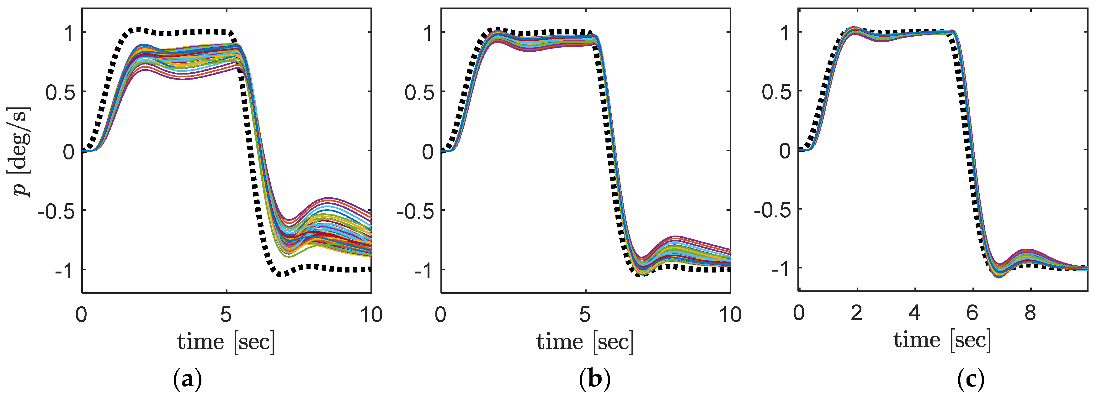
Figure 17. Roll rate p variations with time responses for 64 cruise conditions using (a) PID, (b) PID and DI and (c) PID–DI–NN controller configurations. The dotted line corresponds to the reference roll rate signal, while the coloured lines correspond respectively to the roll rate response for each flight condition.
Aerospace 13 00318 g017
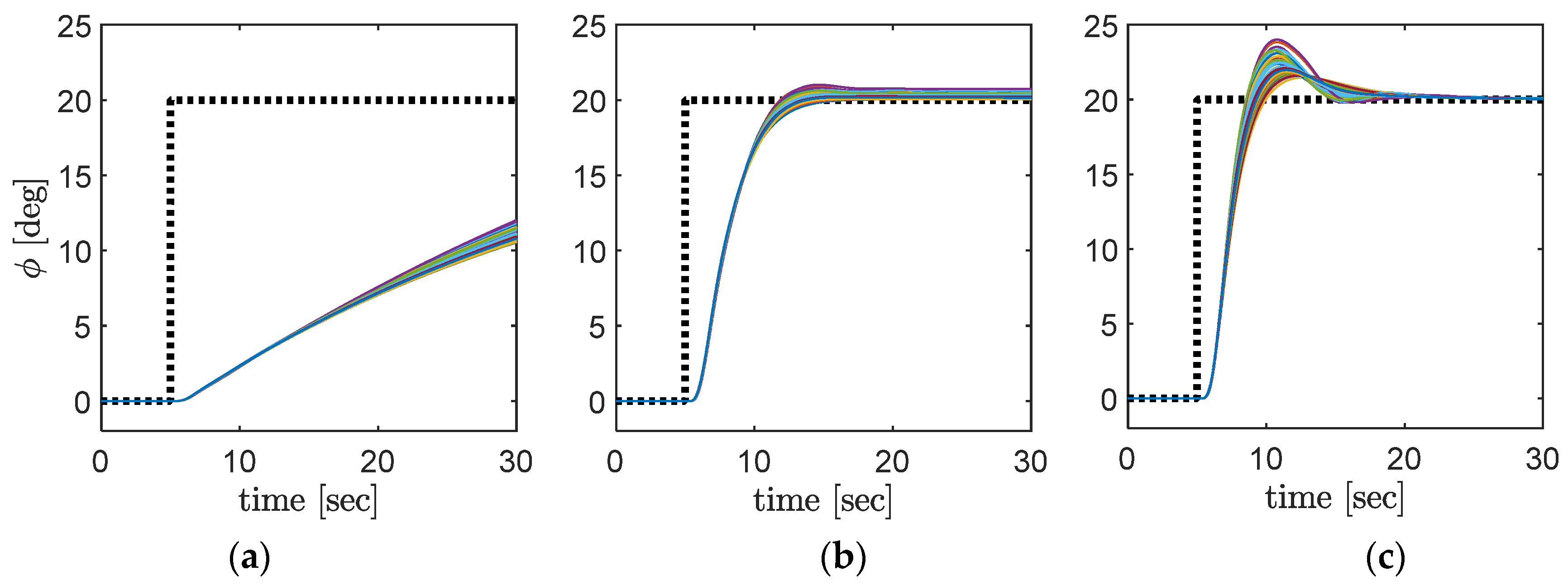
Figure 18. Roll ϕ variation with time responses for 64 cruise conditions for (a) PID, (b) PID–DI and (c) PID–DI–NN controller configurations. The dotted line corresponds to the reference roll angle signal, while the coloured lines correspond respectively to the roll angle response for each flight condition.
Aerospace 13 00318 g018
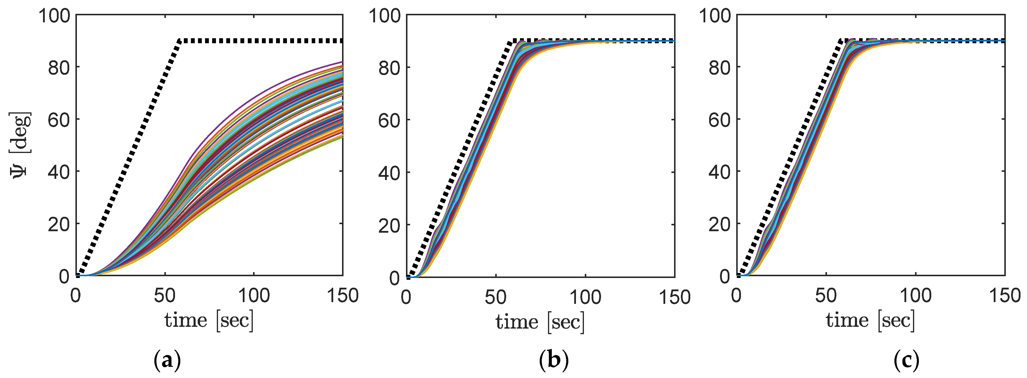
Figure 19. Heading control for 64 cruise conditions for (a) PID, (b) PID–DI and (c) PID–DI–NN controller configurations. The dotted line corresponds to the reference heading signal, while the coloured lines correspond respectively to the heading response for each flight condition. The same reference signal was applied for the three configurations (ac).
Aerospace 13 00318 g019
Figure 20. (a) Dryden turbulence profile and (b) wind-gust profile. The wind profiles show the longitudinal u , lateral v and vertical w wind components.
Aerospace 13 00318 g020
Figure 21. Dual altitude and heading command for 64 representative cruise conditions in the presence of (a) turbulence and (b) wind gusts. The dotted line corresponds to the reference altitude and heading signals, while the coloured lines correspond respectively to the altitude and heading response for each flight condition.
Aerospace 13 00318 g021
Figure 22. Altitude and heading time variation comparison between (a) flight simulations in the RAFS and (b) Simulink simulations. The dotted line corresponds to the reference altitude and heading signals, while the colored lines correspond respectively to the altitude and heading response for each simulated cruise condition.
Aerospace 13 00318 g022
Table 1. Cessna Citation X performance characteristics.
PerformanceMaximum Value
Cruise speed648 km/h [350 knots]
Mach number0.92
Range5725 km [3091 nm]
Altitude15,544 m [51,000 ft]
Takeoff weight16,193 kg [35,700 lb]
Zero-fuel weight11,067 kg [24,400 lb]
Gross thrust28,655 N [6442 lbf]
Table 2. CSAS and autopilot design specifications.
CSAS/AutopilotControlled StateLimitationsSpecifications
Pitch Rate CSAS q ±1.2°/s [±0.0017 rad/s]Smooth and controlled longitudinal maneuvers; Level 1 flight quality.
Vertical-Speed Autopilot V Z ±9.14 m/s [±1800 ft/min] Ensures safe climb and descent rates while allowing rapid altitude changes in emergencies.
Altitude Autopilot h no overshootEnhances safety and passenger comfort during climb/descent transitions.
Roll Rate CSAS p ±2.5°/s [0.43 rad/s]Guarantees smooth, controlled lateral maneuvers; Level 1 flight quality.
Roll Angle CSAS ϕ ±27.5° [0.47 rad]Maintains safe load factors and prevents structural overstress.
Heading Autopilot Ψ heading rate of 3°/s [0.052 rad/s]Complies with civil and military standard turn rates.
Table 3. Second-order nonlinear actuator dynamics.
CharacteristicsValues
Natural frequency 20 rad/s
Maximum deflection 14°
Minimum deflection −19°
Damping ratio 0.8
Rate limit20°/s
Table 4. RLS estimation algorithm and covariance matrix update.
Initialize Θ 0 , L 0
Set κ and ϵ t r e s h o l d
Compute Θ ^ k using Equation (14)
Compute Δ x ^ k + 1 using Equation (12)
Compute ϵ k using Equation
Update L k
if abs ( ϵ k ) ϵ t r e s h o l d
then  L k = 10 3 I
else compute L k using Equation (15)
Table 5. Pitch rate CSAS controller design equations.
Control ElementsEquations
Pitch rate reference model q r e f q c m d = ω s p 2 ( 1 + T θ 2 s ) s 2 + 2   ξ s p ω s p s + ω s p 2
Pitch rate error dynamics e q = q r e f q
NN1 controller input vector x ¯ 1 = q q r e f V z V z c m d δ e T
NN1 adaptation laws W ˙ q = σ σ V 1 T x ¯ 1   e V z T + λ   e V z W q   Γ q
W ˙ V z = σ σ V 1 T x ¯ 1   e V z T + λ   e V z   W V z   Γ V z
V ˙ 1 = Γ V 1 [ x ¯ 1 e V z W V z T σ + x ¯ 1 e q W q T σ + λ e V z + e q V 1 ]
PID controller ν P I D q = K P + K I s + K D s e q
NN1 output signals ν 1 q = K N N q W q T σ V 1 T x ¯ 1
ν 1 V z = K N N V z W V z T σ V 1 T x ¯ 1
Elevator control law Δ δ e = C q G ^ k 1 q ˙ r e f + K P + K I s + K D s e q C q F ^ k Δ x k K N N q W q T σ V 1 T x ¯ 1 (23)
Table 6. Vertical-speed autopilot design equations.
Control ElementsEquations
Error dynamics e V z = V z c m d V z
PID controller output ν P I D V z = K P + K I s + K D   s   e V z
NN1 controller See Table 5
Pitch rate command q c m d   = ν 1 V z   ν P I D V z (24)
Table 7. Altitude autopilot design equations.
Control ElementsEquations
Error dynamics e ¯ h = K e h ( h r e f h )
e ¯ h ˙ = K e h ˙ h ˙
NN2 inputs x ¯ 2 = h h r e f δ e T
NN2 adaptation laws W ˙ h = σ σ V 2 T x ¯ 2 e ¯ h T + λ e ¯ h W h Γ h
W ˙ h ˙ = σ σ V 2 T x ¯ 2 e ¯ h ˙ T + λ e ¯ h ˙ W h ˙ Γ h ˙
V ˙ 2 = Γ V 2 [ x ¯ 2 e ¯ h W h T σ + x ¯ 2 e ¯ h ˙ W h ˙ T σ + λ e ¯ h + e ¯ h ˙ V 2 ]
PID controller ν P I D h = K P + K I s + K D s e h
Feedforward controller ν F F h = K F F h h r e f
NN2 output signals ν 2 h = K N N h W h T σ V 2 T x ¯ 2
ν 2 h ˙ = K N N h ˙ W h ˙ T σ V 2 T x ¯ 2
Command law V z c m d = ( K F F h + ν a d h ˙ ) h ˙ r e f + ν P I D h + d d t ν 2 h (25)
Table 8. Roll rate CSAS controller design equations.
Control ElementsEquations
Roll rate reference model p r e f p c m d = ω d r 2 s 2 + 2 ξ d r ω d r s + ω d r 2 1 τ s + 1
Error dynamics e p = p r e f p
e r = β ˙
NN3 inputs x ¯ 3 = p p r e f δ a δ r T
NN3 adaptation laws W 3 ˙ δ a = σ σ V 3 T x ¯ 3 e p + λ e p W δ a Γ δ a
W 3 ˙ δ r =   σ σ   V 3 T x ¯ 3   e r + λ   e r   W 3 δ r Γ δ r
V ˙ 3 = Γ V 3 [ x ¯   e p W a T   σ + x ¯ e r W r T σ + λ e p + e r V 3 ]
PID controller ν P I D p = K P + K I s + K D s e p
Feedforward controller ν F F p = K F F   p ˙ r e f
Yaw rate washout filter F s = K W F   τ   s τ s + 1
NN3 outputs ν 3 δ a = W a T σ   V 3 T   x ¯ 3
ν 3 δ r = W 3 δ r T σ   V 3 T   x ¯ 3  
Aileron control law Δ δ a k = ( C p G ^ δ a k ) 1 K F F p ˙ r e f + K P + K I s + K D s e p C p F ^ k Δ x k C p G ^ δ r k Δ δ r k 1 W a T σ V 3 T x ¯ 3 (27)
Rudder control law Δ δ r k = ( C r G ^ δ r k ) 1 K W F . τ s τ s + 1 r C r F ^ k Δ x k C r G ^ δ a k Δ δ a k 1 W 3 δ r T σ V 3 T x ¯ 3 + ν 4 δ r k (28)
Table 9. Roll angle CSAS controller design equations.
Control ElementsEquations
Error dynamics e ϕ = ϕ c m d ϕ
NN4 inputs x ¯ 4 = ϕ ϕ c m d Ψ Ψ r e f δ a δ r T
PID controller ν P I D ϕ = K P + K I s + K D s e ϕ
NN4 adaptation laws W 4 ˙ δ r = σ σ V 4 T x ¯ 4 e ϕ T + λ e ϕ W 4 δ r Γ 4 δ r
W ˙ ϕ = σ σ V 4 T x ¯ 4 e ϕ T + λ e ϕ W ϕ Γ ϕ
W ˙ Ψ = σ σ V 4 T x ¯ 4 e ¯ Ψ T + λ e ¯ Ψ W Ψ Γ Ψ
V ˙ 4 = Γ V 4 [ x ¯ 4 e ϕ W ϕ T σ + x ¯ 4 e ¯ Ψ W Ψ T σ + λ e ϕ + e ¯ Ψ V 4 ]
NN4 outputs ν 4 δ r = K N N δ r W 4 T δ r σ V 4 T x ¯ 4
ν 4 ϕ = K N N ϕ W ϕ T σ V 4 T x ¯ 4
ν 4 Ψ = K N N Ψ W 4 Ψ T σ V 4 T x ¯ 4
Command law p c m d = ( C ϕ G ^ δ a k ) 1 ν P I D ϕ C ϕ F ^ k Δ x k + ν 4 ϕ (29)
Table 10. Heading autopilot design equations.
Control ElementsEquations
Error dynamics e Ψ = Ψ r e f Ψ
e ¯ Ψ = K e Ψ e Ψ
PID controller ν P I D Ψ = K P + K I s + K D s e Ψ
Feedforward controller ν F F Ψ = K F F Ψ Ψ ˙ r e f
Command law ϕ c m d = ( C Ψ G ^ δ a k ) 1 ν F F Ψ + ν P I D Ψ C Ψ F ^ k Δ x k + ν 4 Ψ (30)
Table 11. Longitudinal CSAS and autopilot design parameters.
Control ElementsParametersValues
q PID controller K P , K I , K D 1 , 1 , 0.1
RLS longitudinal state estimation κ , L 0 , F ^ 0 , G ^ 0
ϵ q t r e s h o l d , ϵ θ t r e s h o l d
L u p d a t e
1.015 , 1 0 7 I 5 , 5 , I 4 , 4 , 0.1 4 , 1
0.0001 rad/s 0.005 rad
10 4
NN1 controller K N N q , learning rate Γ q
K N N V z , learning rate Γ V z
hidden layers, neurons
5 , 1
0.02, 0.8
1 , 30
Pitch rate reference model ξ s p , ω s p , T θ 2 0.69 , 4 rad/s, 0.35 s
V z PID controller K P , K I , K D 0.1 , 0 , 0
h PID controller K P , K I , K D 0.3 , 0 , 0
h feedforward controller K F F h 0.2
NN2 controller K N N h , K N N h ˙ ,
learning rates Γ h , Γ h ˙ , Γ V 2
K e h , K h ˙ ,
hidden layers, neurons
2, 0.05
1, 1, 2
0.001 , 0.0002
1, 30
Table 12. Lateral CSAS and autopilot design parameters.
Control ElementsParametersValues
p PID controller K P , K I , K D −1, −1, 0
p feedforward controller K F F p −0.1
Yaw damper, washout filter K W F , τ 3, 2 s
NN3 controllerlearning rates Γ a , Γ r , Γ V 3 , λ
number of layers
number of neurons
0.1, 0.3, 2, 1
1
30
p reference model ξ d r , ω d r , τ 0.5, 3 rad/s, 0.5
RLS lateral state estimation κ , L 0 , F ^ 0 , G ^ 0
ϵ p t r e s h o l d , ϵ r t r e s h o l d
L u p d a t e
1.015 , 1 0 4 I 7 , 7 , I 5 , 5 , 0.1 5 , 2
0.0001 rad/s, 0.001 rad/s
10 4 I 7 , 7
ϕ PID controller K P , K I , K D 0.03, 0, 0
Ψ PID controller K P , K I , K D 0.2, 0, 0.1
Ψ feedforward controller K F F Ψ
NN4 controller K N N δ r , K N N ϕ , K N N Ψ , K e Ψ
learning rates Γ δ r , Γ ϕ , Γ ψ ,   Γ V N N 4 , λ
hidden layers, neurons
0.001, 0.0001, 0.005, 0.1
0.5, 4, 4, 1,
1, 1
1, 30
Table 13. CSAS and autopilot transient performance results.
SignalDampingFrequency, rad/sRising Time, sSettling Time, sOvershoot, %
Pitch rate controller0.59–0.774.3–5.3 0.25–0.291–1.856–28
Roll rate controller0.33–0.472.8–3.031.37–1.491.5–3.54.3% <
Roll angle controller --8–1013.2–15.27.2–20
Vertical-speed autopilot--5–810–15 11–34
Altitude autopilot--2.8–4.83.4–6.71% <
Heading autopilot --3.5–233–311% <
Disclaimer/Publisher’s Note: The statements, opinions and data contained in all publications are solely those of the individual author(s) and contributor(s) and not of MDPI and/or the editor(s). MDPI and/or the editor(s) disclaim responsibility for any injury to people or property resulting from any ideas, methods, instructions or products referred to in the content.