A Normalized Objective Function for Multi-Stage Rotor Assembly Optimization Targeting Vibration Suppression Across Critical Speeds

Abstract

Excessive vibration during critical speed traversal remains a primary challenge in assembling multi-stage rotors of aero-engines. Conventional assembly optimization methods, which target static geometric and mass eccentricity errors or vibration at a fixed operating speed, are inadequate to ensure smooth passage through multiple critical speeds. To address this gap, we propose a novel, vibration-suppression-oriented assembly optimization model. A normalized objective function is formulated to minimize the overall vibration response across multiple rotor nodes specifically at the first and second critical speeds. This function integrates an assembly error propagation model with a rotor dynamic model that considers flexible dynamic deflection. The optimal assembly angle sequence is solved using a genetic algorithm. Experimental validation on a four-stage rotor demonstrates that the proposed method reduces the maximum vibration displacement amplitude at the first and second critical speeds by 74.7% and 11.9%, respectively, significantly outperforming conventional objectives based on geometric error, unbalanced mass, or single-speed vibration. This work provides a practical and effective strategy to enhance rotor dynamic safety by ensuring low-vibration operation across the critical speeds encountered before reaching the operating speed through optimal assembly.

1. Introduction

The multi-stage rotor is the most critical component in large-scale rotating machinery, such as aero-engines and gas turbines. The post-assembly vibration response serves as the paramount indicator for evaluating its assembly quality [1,2]. In recent years, significant research efforts have been devoted to developing optimization methods for the assembly angles of multi-stage rotors. These methods aim to minimize geometric and unbalanced mass errors in the assembled rotor by optimally matching the assembly angles of each single-stage rotor, based on measured geometric and mass characteristic parameters.

Hussain and Yang et al. [3,4,5,6,7,8,9] pioneered an assembly error propagation model for axi-symmetric rotational components. By defining tolerance zones for key dimensions of each single-stage rotor, statistical methods were employed to evaluate the geometric eccentricity error of the multi-stage rotor under all possible assembly angle combinations. These methods essentially constitute tolerance analysis, providing guidance for tolerance allocation during the rotor design stage. However, they cannot directly yield the optimal assembly angles that minimize the geometric eccentricity error of the assembled rotor.

Wang and Sun et al. [10,11,12] developed a measurement model for multi-stage rotor assembly error based on the positional and orientational deviations of individual single-stage rotors. This model takes the final coaxiality of the assembled rotor as the optimization objective to determine the optimal assembly angles for each stage. Sun et al. [13] also proposed an assembly angle correction method for aero-engine rotors based on geometric eccentricity minimization, whose theoretical foundation aligns with that presented in Ref. [10]. Ding et al. [14] introduced a REM–GA rotor assembly optimization method. This method utilizes a robust eigenvalue method to convert point cloud data from rotor assembly faces into plane parameter equations, determining the optimal relative assembly angle between adjacent rotors based on their tilt and offset relationships. Sun et al. [15,16] further incorporated the Jacobian–Torsor theory into the aforementioned propagation model to analyze the transmission patterns and interactive effects of cumulative geometric errors in multi-stage rotors. Tu et al. [17] established an assembly error propagation model based on geometric algebra theory, which reportedly offers significantly improved computational efficiency compared to traditional homogeneous transformation matrix models. Liu et al. [18] applied the centroid coordinate transfer method from Ref. [10] to the transfer of mass center coordinates. However, in this method, the mass center coordinates are not obtained through direct measurement but are estimated from the geometric centroid coordinates of each single-stage rotor using an assumed conversion factor, which constitutes a significant limitation. To address this deficiency, we employed a horizontal balancing machine to directly measure the two-plane unbalance of each single-stage rotor and proposed a dual-objective optimization method targeting both coaxiality and unbalance for multi-stage rotors using a genetic algorithm [19].

Sun et al. [20,21,22], building upon the multi-stage rotor assembly error propagation model from ref. [10], derived a mathematical model describing how the unbalance excitation force of each single-stage rotor varies with assembly angles. They further formulated an objective function based on the vibration displacement at the bearings under the rotor’s operating speed to solve for the optimal assembly angles. Results indicated that for a four-stage rotor, the optimal assembly angles reduced bearing-end vibration displacement by 29.8%, 19.6%, and 22.0% at 3000 rpm, 6000 rpm, and 9000 rpm, respectively, compared to the default assembly. Subsequently, we established an optimization function with the maximum vibration velocity at the front and rear journal bearings as the objective and the assembly angles of the single-stage rotors as variables. Experimental verification demonstrated that the optimal assembly significantly reduced the vibration velocity at the bearings by 69.6% and 45.5% compared to the worst-case and default assemblies, respectively [23].

While extensive research has focused on optimizing assembly angles to minimize geometric errors and unbalance, the fundamental question of why assembly angles matter from a dynamics perspective warrants further examination. In multi-stage rotor systems, the assembly configuration determines not only the static alignment of components but also the dynamic interactions between stages under operating conditions.

Bladh et al. [24] investigated the effects of multistage coupling and disk flexibility on the dynamics of bladed disks, demonstrating that proper treatment of interstage boundaries is essential for capturing disk-blade modal interactions, particularly in eigenfrequency veering regions. Their findings revealed that multistage coupling-induced changes in disk flexibility significantly impact both tuned forced responses and a design’s sensitivity to mistuning. This suggests that assembly configurations, which inherently affect the relative positioning of stages, can influence the dynamic coupling between components and consequently the forced vibration characteristics of the entire rotor system.

Similarly, Shahab and Thomas [25] examined the coupling effects of disk flexibility on the dynamic behavior of multi-disk-shaft systems, showing that disk flexibility introduces additional degrees of freedom that modify the system’s modal properties. These effects are particularly relevant for assembled rotors, where the interface conditions between stages determine how flexibility propagates through the assembly.

Laxalde et al. [26] developed a method for dynamical analysis of multistage cyclic structures, highlighting that interstage coupling must be properly accounted for when predicting the forced response of turbomachinery rotors. Their work demonstrated that engine-order excitations can propagate through stage interfaces, making the assembly configuration a critical factor in determining vibration amplitudes at resonant conditions.

Rzadkowski and Maurin [27] further extended this analysis to mistuned bladed disk assemblies on flexible shafts, considering forced vibrations under various engine-order excitations. Their results showed that multistage coupling significantly influences stress distributions and resonance conditions, with assembly-induced variations in stage alignment potentially altering the forced response characteristics.

These studies collectively underscore that assembly angles are important not merely for static alignment but because they govern the dynamic coupling between stages, influencing the system’s forced vibration behavior at critical operating conditions. As noted in [24], multistage analyses may be required when excitations are expected to fall in or near eigenfrequency veering regions—precisely the conditions encountered during critical speed traversal. Therefore, a comprehensive assembly optimization approach must consider not only static eccentricity errors but also the forced vibration response of the assembled system, which is the central objective of the present work.

In summary, the multi-stage rotor assembly angle optimization process enables the minimization of geometric errors, unbalanced mass errors, or vibration responses of the assembled rotor by using the assembly angles of each single-stage rotor as control variables, without requiring secondary corrective machining. The primary distinctions among existing studies lie in three aspects of their formulated objective functions:

• Choice of the objective function: Optimization models have evolved from initially considering only geometric properties to incorporating mass properties, and finally to directly targeting vibration response. The optimization of multi-stage rotor vibration has thus progressed from an indirect to a direct approach, establishing a direct functional relationship between assembly angles and vibration response.
• Rotational speed in the objective function: The operational speeds of multi-stage high-pressure rotors in modern high-bypass-ratio civil aero-engines commonly exceed the first critical speed, with some even surpassing the second critical speed. However, existing studies targeting vibration response have exclusively used the vibration response at the operational speed as the objective function. The resulting optimal assembly angles may minimize vibration at the operating speed but do not necessarily ensure that the rotor smoothly traverses the first two critical speeds without interacting with the stator casing. Increasing the radial clearance between the rotor and stator to mitigate this risk would significantly reduce compressor efficiency. Therefore, sacrificing engine efficiency by enlarging radial clearance to ensure safe passage through critical speeds is not a viable solution. The rotational speeds considered in the objective function should instead be the multiple critical speeds encountered before reaching the operating speed.
• Node selection in the objective function: Existing studies targeting vibration response have used the single-node vibration displacement amplitude at the rotor bearings as the objective function. The resulting optimal assembly angles may minimize vibration at this specific target node but cannot guarantee a simultaneous reduction—and may even cause an increase—in the vibration response at other nodal locations on the rotor. Consequently, an objective function capable of characterizing the overall vibration level of the entire rotor should be established.

Addressing the aforementioned research gaps, this study builds upon our previously developed and experimentally validated multi-stage rotor assembly error propagation model and dynamic model considering flexible dynamic deflection. In Section 2, by establishing the functional relationship between the assembly angle sequence and the nodal vibration responses, a normalized objective function is formulated to minimize the overall vibration response of the rotor system across multiple critical speeds. In Section 3.1, a genetic algorithm is employed to solve for the optimal assembly angles of the single-stage rotors under three different objective functions constructed in this work. In Section 3.2, a comparative analysis is conducted on the effectiveness of the three proposed objective functions versus those from existing studies for suppressing rotor vibration at the first and second critical speeds. Experimental verification in Section 4 demonstrates that, compared to the default assembly angle set, the optimal assembly angle set obtained using the proposed normalized vibration response objective function reduces the maximum displacement amplitude across six nodes at the first and second critical speeds by 74.7% and 11.9%, respectively. This vibration suppression effect is significantly superior to that achieved by the four objective functions from existing studies.

2. Methods

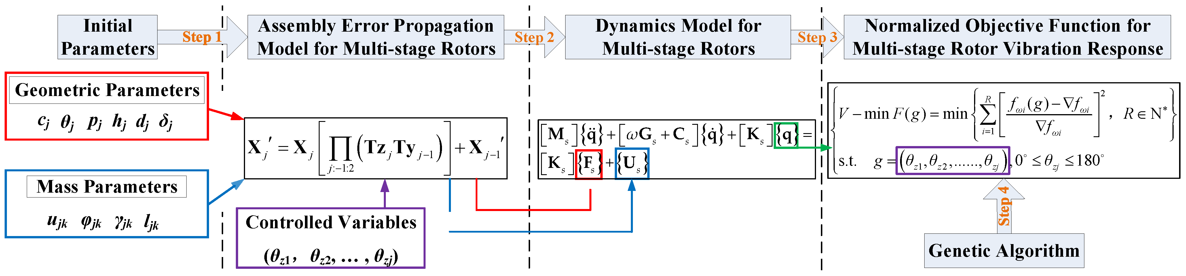
To evaluate the overall vibration level of a multi-stage rotor under different assembly angle sequences and establish a quantifiable objective for optimization, it is necessary to construct an objective function that reflects the vibration responses at all nodes of the rotor. The construction of this function follows a clear relational chain, as illustrated in Figure 1.

2.1. Measurement Definition of Geometric Parameters for a Single-Stage Rotor

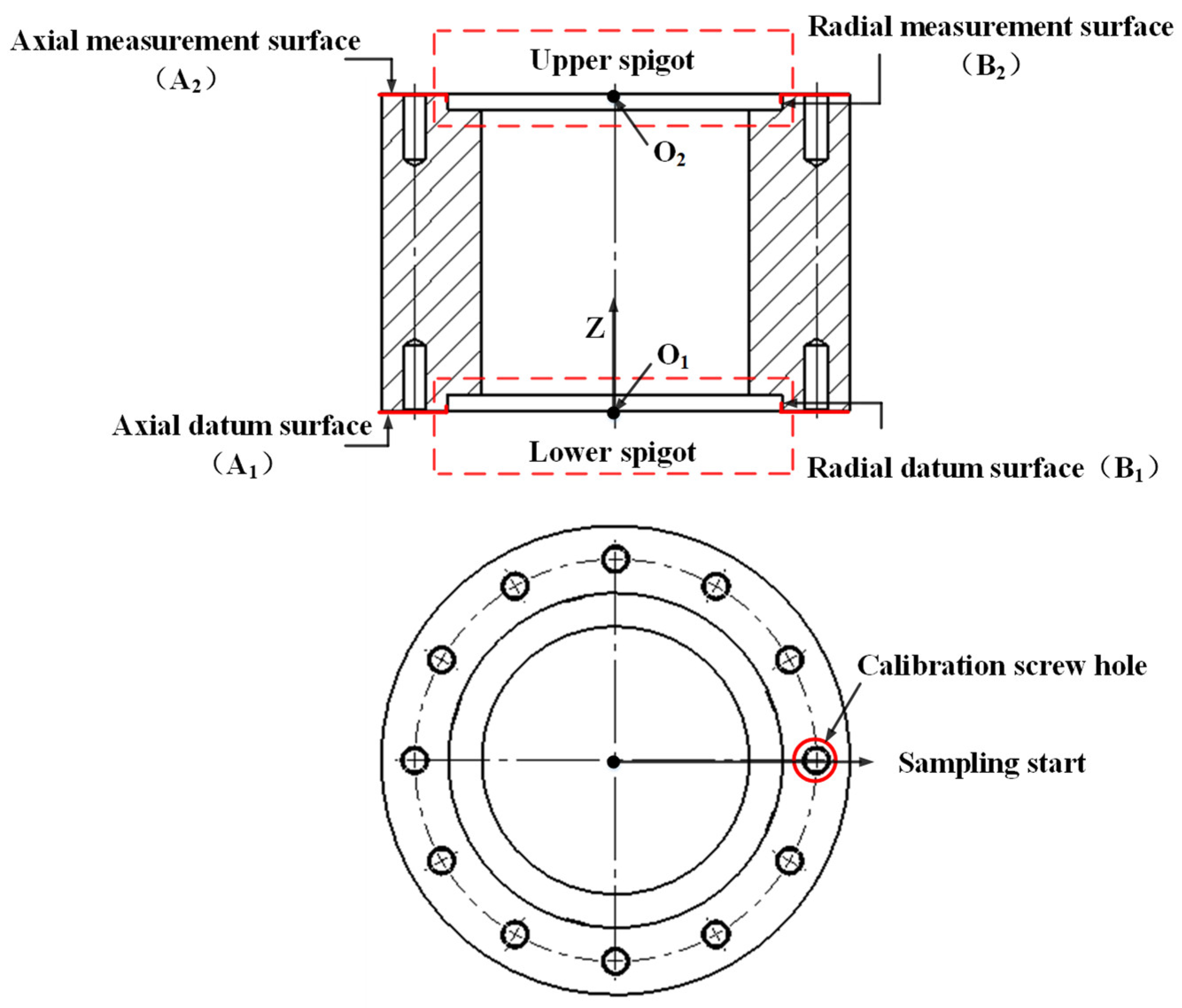
Figure 2 illustrates the measurement definition of the assembly spigot for a single-stage rotor. The measurement procedure using a coordinate measuring machine (CMM) is as follows:

Step 1: Evenly distribute probing points on the axial datum surface of the lower spigot, and fit plane A₁ as the XY plane.

Step 2: Evenly distribute probing points along the radial datum surface (surface B₁) of the lower spigot, fit a circle and its centroid, and define the line passing through this centroid and perpendicular to the XY plane as the Z-axis.

Step 3: Project the fitted circle and its centroid from Step 2 onto the XY plane along the Z-axis and define the projected centroid O₁ as the coordinate origin.

Step 4: Measure the parallelism error and the vertical distance between surface A₂ and surface A₁. Select any pair of assembly screw holes with the same distribution angle on the circumference of the upper and lower assembly surfaces as the calibration screw holes. Choose one of these holes, probe four points to calibrate its center, and define the line connecting this center to the Z-axis as the sampling start direction (0°). From this sampling start angle, establish evenly distributed measurement points on surface A₂ and fit surface A₂. The mean value of the Z-coordinates of the fitted surface A₂ at all sampling angles represents the vertical distance between surface A₂ and surface A₁. The difference between the highest and lowest points represents the parallelism error between surface A₂ and surface A₁. The line connecting the highest and lowest points, projected onto surface A₁, is defined as the X-axis.

Step 5: Measure the eccentricity error between surface B₂ and surface B₁. Establish evenly distributed measurement points on surface B₂, fit a circle and its centroid, and project them onto surface A₂. Define the projected centroid as O₂. The eccentricity and eccentricity angle between surface B₂ and surface B₁ can be obtained from the spatial coordinates of O₁ and O₂.

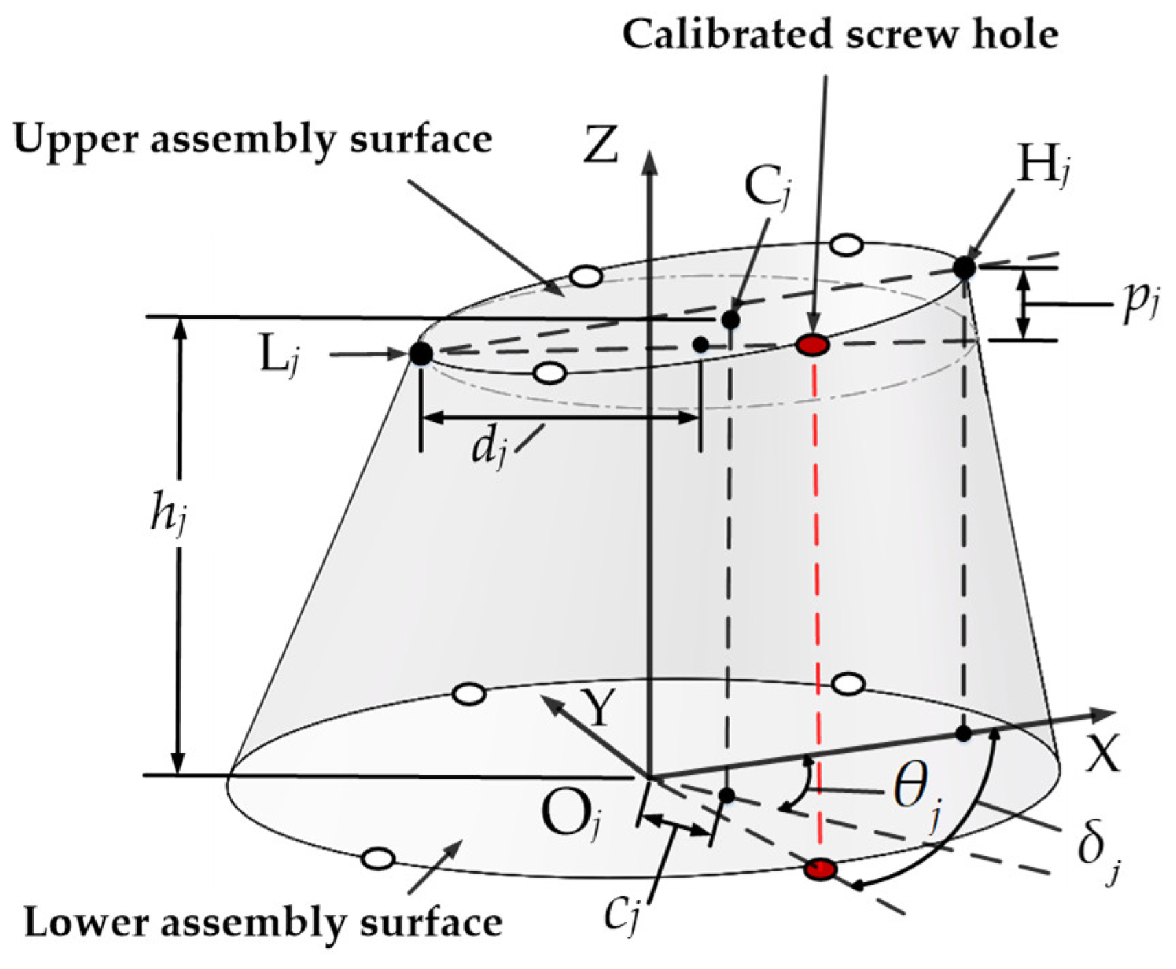
Figure 3 illustrates all the geometric parameters to be measured for a single-stage rotor, along with the measurement coordinate system. The lower assembly surface of the j-th stage rotor is defined as the XY plane of the measurement coordinate system (Step 1). The axis passing through the spigot centroid O_j and perpendicular to the lower assembly surface is defined as the Z-axis (Step 2). The spigot centroid O_j is defined as the coordinate origin (Step 3). The projection of the line connecting the highest point H_j and the lowest point L_j of the upper assembly surface onto the lower assembly surface is defined as the X-axis. δ_j is the sampling angle between the center of the calibrated screw hole and H_j. h_j is the vertical distance between the upper and lower assembly surfaces, and p_j is the parallelism error between these surfaces (Step 4). c_j and θ_j are the eccentricity distance and eccentricity angle of the centroid C_j of the upper assembly surface, respectively (Step 5). Its coordinate vector can be expressed as C_j = [c_jcos(θ_j), c_jsin (θ_j), h_j]. The radius d_j of the upper assembly surface can be obtained from the circle fitted in Step 5.

2.2. Measurement Definition of Mass Parameters for a Single-Stage Rotor

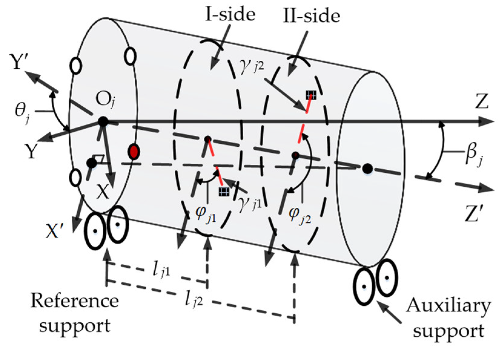
A dynamic balancing machine is employed to measure the mass parameters of a single-stage rotor, including the two-plane unbalance mass, its action phase, and the action radius of the unbalanced mass points. The measurement definition is shown in Figure 4. The procedure is as follows:

Step 1: Place the rotor to be measured on the bilateral pendulum supports of the dynamic balancing machine. The upper and lower assembly surfaces in the geometric measurement coordinate system should preferably be positioned on the left and right roller supports. If the spigot structure (e.g., a concave spigot) does not permit this or falls outside the adjustment range of the support rollers, alternative support benchmarks should be considered during the machining process.

Step 2: Define the eccentric direction of the centroid of the lower assembly surface of the j-th stage rotor as the zero phase.

Step 3: Align the phase of the calibrated screw hole with the key-phase sensor.

Step 4: Rotate the rotor by δ_j − θ_j degrees.

Step 5: Attach a reflective sticker at the corresponding position of the key-phase sensor.

After completing the above steps, the dynamic balancing machine can be started to perform the measurement.

In Figure 4, the O_jZ′ axis represents the measurement datum for the mass feature parameters of the j-th stage rotor, i.e., its actual rotation axis. The coordinates of the unbalanced mass points are measured relative to the coordinate system O_jX′Y′Z′ and need to be further unified into the geometric measurement coordinate system O_jXYZ to ensure the synchronous transmission of both types of parameters in the assembly model. The coordinate vector I_jk of an unbalanced mass point can be expressed by Equation (1). Using the coordinate transformation Equation (2), I_jk is first rotated by θ_j about the O_jZ-axis and then rotated by β_j (where β_j = arctan(c_j/h_j)) about the O_jY-axis, finally converting I_jk into the coordinate vector E_jk relative to the O_jXYZ coordinate system.

$$I_{jk}=\left[\begin{array}{ccc}{\gamma }_{jk}\cos \left({\phi }_{jk}\right)& {\gamma }_{jk}\sin \left({\phi }_{jk}\right)& l_{jk}\end{array}\right]\left(j,k\in {\mathrm{N}}^{\ast },k\le 2\right),$$

(1)

where φ_jk is the action phase of the k-th unbalanced mass point of the j-th stage rotor; γ_jk is the action radius of the k-th unbalanced mass point of the j-th stage rotor; l_jk is the distance between the k-th unbalanced mass point of the j-th stage rotor and the reference support.

$$E_{jk}=I_{jk}\left[\begin{array}{ccc}\cos \left({\theta }_j\right)& -\sin \left({\theta }_j\right)& 0\\ \sin \left({\theta }_j\right)& \cos \left({\theta }_j\right)& 0\\ 0& 0& 1\end{array}\right]\left[\begin{array}{ccc}\cos \left({\beta }_j\right)& 0& \sin \left({\beta }_j\right)\\ 0& 1& 0\\ -\sin \left({\beta }_j\right)& 0& \cos \left({\beta }_j\right)\end{array}\right].$$

(2)

2.3. Coordinate Transfer for Multi-Stage Rotor Assembly

Using the assembly angles of each single-stage rotor as control variables (denoted as θ_z1, θ_z2,…, θ_zj), these initial parameters are input into our established multi-stage rotor assembly error propagation model (Equation (3)). This model computes the assembly spigot eccentricity errors and mass eccentricity errors, which vary with the assembly angles.

$${X_j}^{\prime }=X_j\left[{\displaystyle \prod _{j:-1:2}\left(T{z}_{j}T{y}_{j-1}\right)}\right]+{X_{j-1}}^{\prime },$$

(3)

where X_j′ is the coordinate vector of X_j after assembly transformation; Tz_j is the coordinate rotation matrix of the j-th stage rotor about the Z-axis (Equation (4)); Ty_j is the coordinate rotation matrix of the j-th stage rotor about the Y-axis (Equation (5)).

$$T{z}_j=\left[\begin{array}{ccc}\cos \left({\theta }_{zj}+{\delta }_j-{\delta }_{j-1}\right)& -\sin \left({\theta }_{zj}+{\delta }_j-{\delta }_{j-1}\right)& 0\\ \sin \left({\theta }_{zj}+{\delta }_j-{\delta }_{j-1}\right)& \cos \left({\theta }_{zj}+{\delta }_j-{\delta }_{j-1}\right)& 0\\ 0& 0& 1\end{array}\right],$$

(4)

where δ_j − δ_j−1 is the actual phase difference between two adjacent rotor stages; θ_zj is the selectable assembly phase of the j-th stage rotor relative to the (j − 1)-th stage rotor. The parameter δ_j represents the angle between the calibrated screw hole of the j-th stage rotor and the X-axis. When the screw holes of adjacent rotors are aligned, the phase difference in the j-th stage rotor relative to the (j − 1)-th stage rotor becomes δ_j − δ_j−1. Thus, when the j-th stage rotor selects any assembly phase θ_zj, the phase difference between the two stages is θ_zj + (δ_j − δ_j−1).

$$T{y}_j=\left[\begin{array}{ccc}\cos \left(\arctan \left({\displaystyle \frac{p_j}{2d_j}}\right)\right)& 0& \sin \left(\arctan \left({\displaystyle \frac{p_j}{2d_j}}\right)\right)\\ 0& 1& 0\\ -\sin \left(\arctan \left({\displaystyle \frac{p_j}{2d_j}}\right)\right)& 0& \cos \left(\arctan \left({\displaystyle \frac{p_j}{2d_j}}\right)\right)\end{array}\right].$$

(5)

2.4. Mass Eccentricity Errors of a Multi-Stage Rotor Based on Its Actual Rotation Axis

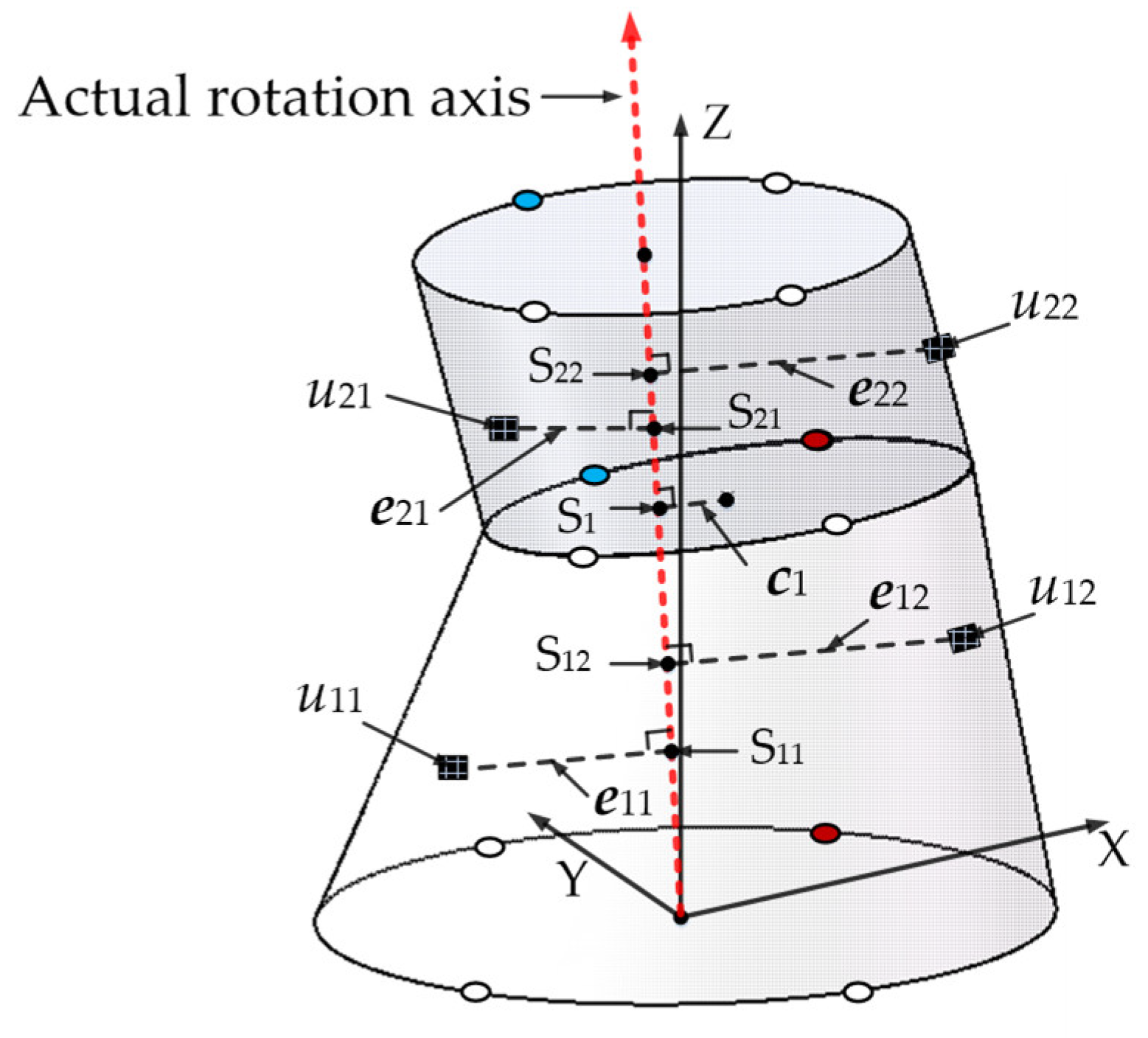
During the assembly process of a multi-stage rotor, the inherent errors of each single-stage rotor are transmitted step-by-step through the assembly spigots, forming cumulative errors. This consequently causes the actual spatial positions of the rotors at each stage to deviate from their ideal assembly positions, and the actual rotation axis of the assembly to deviate from the geometric reference axis. Therefore, the geometric and mass eccentricity errors of the rotors at each stage should be recalculated relative to the actual rotation axis, based on the centroid coordinates after assembly transformation and the coordinates of the unbalanced mass points. The actual rotation axis itself also changes with variations in the assembly phases of the rotors at each stage. Figure 5 illustrates the geometric and mass eccentricity errors of a two-stage rotor under a specific assembly phase. The actual rotation axis is the line connecting the centroids of the supporting journal cross-sections of the first and last rotors. Let the coordinate vectors of the spigot centroid and the k-th unbalanced mass point of the j-th stage rotor before assembly be C_j = [C_jx, C_jy, C_jz] and E_jk = [E_jkx, E_jky, E_jkz], respectively. Substituting these into Equation (3) yields the coordinates after assembly, C_j′ = [C_jx′, C_jy′, C_jz′] and E_jk′ = [E_jkx′, E_jky′, E_jkz′]. The linear parameter equation of the actual rotation axis can then be expressed as

$${\displaystyle \frac{x}{{C_{jx}}^{\prime }}}={\displaystyle \frac{y}{{C_{jy}}^{\prime }}}={\displaystyle \frac{z}{{C_{jz}}^{\prime }}}=\lambda .$$

(6)

The equation of the normal plane passing through the k-th unbalanced mass point of the j-th stage rotor and perpendicular to the rotation axis is:

$${C_{jx}}^{\prime }\left(x-{E_{jkx}}^{\prime }\right)+{C_{jy}}^{\prime }\left(y-{E_{jky}}^{\prime }\right)+{C_{jz}}^{\prime }\left(z-{E_{jkz}}^{\prime }\right)=0.$$

(7)

By combining Equations (6) and (7), the parameter λ of the linear equation can be obtained as:

$$\lambda ={\displaystyle \frac{{C_{jx}}^{\prime }{E_{jkx}}^{\prime }+{C_{jy}}^{\prime }{E_{jky}}^{\prime }+{C_{jz}}^{\prime }{E_{jkz}}^{\prime }}{{\left({C_{jx}}^{\prime }\right)}^2+{\left({C_{jy}}^{\prime }\right)}^2+{\left({C_{jz}}^{\prime }\right)}^2}}.$$

(8)

Substituting λ into Equation (6) yields the coordinates of the intersection point S_jk between the rotation axis and the normal plane:

$$\left\{\begin{array}{c}{S}_{jkx}={\displaystyle \frac{{\left({C_{jx}}^{\prime }\right)}^2{E_{jkx}}^{\prime }+{C_{jx}}^{\prime }{C_{jy}}^{\prime }{E_{jky}}^{\prime }+{C_{jx}}^{\prime }{C_{jz}}^{\prime }{E_{jkz}}^{\prime }}{{\left({C_{jx}}^{\prime }\right)}^2+{\left({C_{jy}}^{\prime }\right)}^2+{\left({C_{jz}}^{\prime }\right)}^2}}\\ S_{jky}={\displaystyle \frac{{C_{jx}}^{\prime }{C_{jy}}^{\prime }{E_{jkx}}^{\prime }+{\left({C_{jy}}^{\prime }\right)}^2{E_{jky}}^{\prime }+{C_{jy}}^{\prime }{C_{jz}}^{\prime }{E_{jkz}}^{\prime }}{{\left({C_{jx}}^{\prime }\right)}^2+{\left({C_{jy}}^{\prime }\right)}^2+{\left({C_{jz}}^{\prime }\right)}^2}}\\ S_{jkz}={\displaystyle \frac{{C_{jx}}^{\prime }{C_{jz}}^{\prime }{E_{jkx}}^{\prime }+{C_{jy}}^{\prime }{C_{jz}}^{\prime }{E_{jky}}^{\prime }+{\left({C_{jz}}^{\prime }\right)}^2{E_{jkz}}^{\prime }}{{\left({C_{jx}}^{\prime }\right)}^2+{\left({C_{jy}}^{\prime }\right)}^2+{\left({C_{jz}}^{\prime }\right)}^2}}\end{array}\right..$$

(9)

Then, the action radius vector e_jk of the k-th unbalanced mass point of the j-th stage rotor can be expressed as

$$e_{jk}=\left\{\left({E_{jkx}}^{\prime }-S_{jkx}\right),\left({E_{jky}}^{\prime }-S_{jky}\right),\left({E_{jkz}}^{\prime }-S_{jkz}\right)\right\}.$$

(10)

Similarly, the geometric eccentricity vector c_j of the assembly spigot of the j-th stage rotor can be expressed as

$$c_j=\left\{\left({C_{jx}}^{\prime }-S_{jx}\right),\left({C_{jy}}^{\prime }-S_{jy}\right),\left({C_{jz}}^{\prime }-S_{jz}\right)\right\}.$$

(11)

2.5. Decomposition Principle of Two-Plane Unbalance in a Multi-Stage Rotor

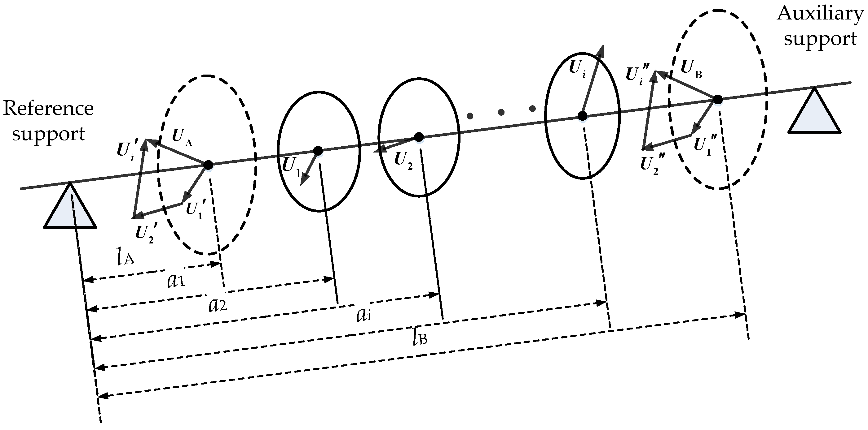
Figure 6 illustrates the decomposition principle of two-plane unbalance in a rotor dynamic balancing test. Assuming there are i unbalance vectors U_i located on i planes perpendicular to the rotation axis, two planes at distances l_A and l_B from the reference support are selected as correction planes. According to the principle of moment balance, U_i is decomposed into two component vectors, U_i′ and U_i″, on planes A and B. The resultant unbalanced vectors U_A and U_A on planes A and B are then the vector sums of U_i′ and U_i″, respectively:

$$\left\{\begin{array}{l}{U}_{\mathrm{A}}={\displaystyle \sum _{i=1}^n\frac{l_{\mathrm{B}}-a_i}{l_{\mathrm{B}}-l_{\mathrm{A}}}{U}_i}\\ U_{\mathrm{B}}={\displaystyle \sum _{i=1}^n\frac{a_i-l_{\mathrm{A}}}{l_{\mathrm{B}}-l_{\mathrm{A}}}{U}_i}\end{array}\right.,$$

(12)

where a_i is the distance between the i-th unbalance vector and the reference support.

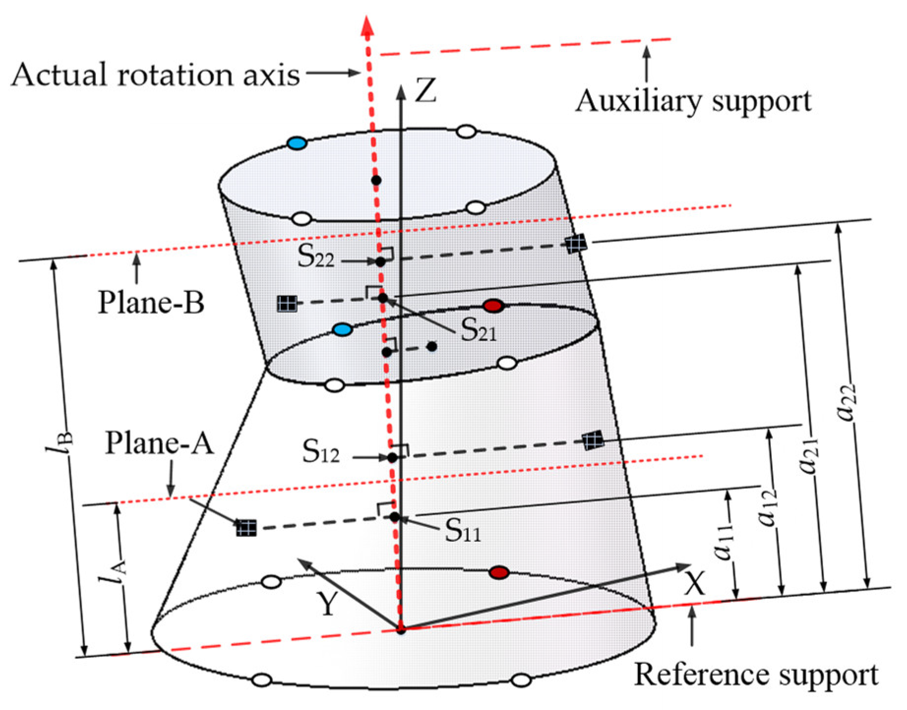
Figure 7 shows a schematic diagram of the two-plane unbalance decomposition for a two-stage rotor. Extending this to a multi-stage rotor, the distance between the k-th unbalanced mass point of the j-th stage rotor and the reference support can be expressed as:

$$a_{jk}=\sqrt{{\left(S_{jkx}\right)}^2+{\left(S_{jky}\right)}^2+{\left(S_{jkz}\right)}^2}.$$

(13)

If the vector direction of the first unbalanced mass point of the first stage rotor is taken as the X-direction, the angle between this direction and that of another unbalanced mass point is:

$${\theta }_{jk\to 1}=\arccos \left({\displaystyle \frac{e_{11}\cdot e_{jk}}{\left|e_{11}\right|\left|e_{jk}\right|}}\right).$$

(14)

According to Equation (12), the unbalance on Plane A of the multi-stage rotor, decomposed from the two-plane unbalance of each stage rotor, can be obtained as:

$$\left\{\begin{array}{l}{U}_{\mathrm{A}x}={\displaystyle \sum _{j=1}^n\left[\frac{l_{\mathrm{B}}-a_{j1}}{l_{\mathrm{B}}-l_{\mathrm{A}}}{u}_{j1}{e}_{j1}\cos \left({\theta }_{j1\to 1}\right)+\frac{l_{\mathrm{B}}-a_{j2}}{l_{\mathrm{B}}-l_{\mathrm{A}}}{u}_{j2}{e}_{j2}\cos \left({\theta }_{j2\to 1}\right)\right]}\\ U_{\mathrm{A}y}={\displaystyle \sum _{j=1}^n\left[\frac{l_{\mathrm{B}}-a_{j1}}{l_{\mathrm{B}}-l_{\mathrm{A}}}{u}_{j1}{e}_{j1}\sin \left({\theta }_{j1\to 1}\right)+\frac{l_{\mathrm{B}}-a_{j2}}{l_{\mathrm{B}}-l_{\mathrm{A}}}{u}_{j2}{e}_{j2}\sin \left({\theta }_{j2\to 1}\right)\right]}\end{array}\right..$$

(15)

where u_jk is the k-th unbalanced mass of the j-th stage rotor, and u_jke_jk is the k-th unbalance (mass–radius product) of the j-th stage rotor. Similarly, the unbalance on Plane B of the multi-stage rotor, decomposed from the two-plane unbalance of each stage rotor, can be obtained as:

$$\left\{\begin{array}{l}{U}_{\mathrm{B}x}={\displaystyle \sum _{j=1}^n\left[\frac{a_{j1}-l_{\mathrm{A}}}{l_{\mathrm{B}}-l_{\mathrm{A}}}{u}_{j1}{e}_{j1}\cos \left({\theta }_{j1\to 1}\right)+\frac{a_{j2}-l_{\mathrm{A}}}{l_{\mathrm{B}}-l_{\mathrm{A}}}{u}_{j2}{e}_{j2}\cos \left({\theta }_{j2\to 1}\right)\right]}\\ U_{\mathrm{B}y}={\displaystyle \sum _{j=1}^n\left[\frac{a_{j1}-l_{\mathrm{A}}}{l_{\mathrm{B}}-l_{\mathrm{A}}}{u}_{j1}{e}_{j1}\sin \left({\theta }_{j1\to 1}\right)+\frac{a_{j2}-l_{\mathrm{A}}}{l_{\mathrm{B}}-l_{\mathrm{A}}}{u}_{j2}{e}_{j2}\sin \left({\theta }_{j2\to 1}\right)\right]}\end{array}\right..$$

(16)

The two-plane unbalance of the multi-stage rotor can then be determined using Equation (17), and its action phase can be expressed by Equation (18):

$$\left\{\begin{array}{l}{U}_{\mathrm{A}}=\sqrt{{\left(U_{\mathrm{A}x}\right)}^2+{\left(U_{\mathrm{A}y}\right)}^2}\\ U_{\mathrm{B}}=\sqrt{{\left(U_{\mathrm{B}x}\right)}^2+{\left(U_{\mathrm{B}y}\right)}^2}\end{array}\right..$$

(17)

$$\left\{\begin{array}{l}{\zeta }_{\mathrm{A}}=\arctan \left({\displaystyle \frac{U_{\mathrm{A}y}}{U_{\mathrm{A}x}}}\right)+{\phi }_{11}\\ {\zeta }_{\mathrm{B}}=\arctan \left({\displaystyle \frac{U_{\mathrm{B}y}}{U_{\mathrm{B}x}}}\right)+{\phi }_{11}\end{array}\right..$$

(18)

2.6. Synchronous Excitation of Mass and Spigot Eccentricities in Multi-Stage Rotors

Assuming the multi-stage rotor has n shaft elements and n + 1 nodes, the spigot eccentricity error of the j-th stage rotor acts on node i, and the k-th mass eccentricity error of the j-th stage rotor acts on node f. If the vector direction of the first mass eccentricity error is taken as the measurement direction for the X-direction vibration response, the phase differences between this direction and the nodal excitations generated by all other mass and spigot eccentricity errors can be expressed as

$$\left\{\begin{array}{l}{\theta }_{j\to 1}=\arccos \left({\displaystyle \frac{e_{11}\cdot c_j^i}{\left|e_{11}\right|\left|c_j^i\right|}}\right)\hfill \\ {\theta }_{jk\to 1}=\arccos \left({\displaystyle \frac{e_{11}\cdot e_{jk}^f}{\left|e_{11}\right|\left|e_{jk}^f\right|}}\right)\hfill \end{array}\right.\left(1\le i,f\le n+1,n\in {\mathrm{N}}^{\ast }\right).$$

(19)

The mass eccentricity excitation U_f at node f of the multi-stage rotor is decomposed into the X and Y directions as

$$\left\{\begin{array}{l}{U}_{fx}=u_{jk}^f{\omega }^2\left|e_{jk}^f+r_j^{\omega }\right|\cos \left({\theta }_{jk\to 1}+\omega t\right)\hfill \\ U_{fy}=u_{jk}^f{\omega }^2\left|e_{jk}^f+r_j^{\omega }\right|\sin \left({\theta }_{jk\to 1}+\omega t\right)\hfill \end{array}\right..$$

(20)

The spigot eccentricity excitation F_i at node i of the multi-stage rotor is decomposed into the X and Y directions as

$$\left\{\begin{array}{l}{F}_{ix}=\left|c_j^i+r_j^{\omega }\right|\cos \left({\theta }_{j\to 1}+\omega t\right)\hfill \\ F_{iy}=\left|c_j^i+r_j^{\omega }\right|\sin \left({\theta }_{j\to 1}+\omega t\right)\hfill \end{array}\right..$$

(21)

2.7. Dynamic Equations of a Multi-Stage Rotor System

The mass and spigot eccentricities errors at each node are input into our developed dynamic model for the multi-stage rotor (Equation (22)), where they are transformed into the geometric eccentricity excitation F_s (Equation (23)) and the mass eccentricity excitation U_s (Equation (24)), both being functions of the assembly angles. In (Equation (22)), M_s is the system mass matrix of dimension 4(n + 1) × 4(n + 1), K_s is the system stiffness matrix, and [ωG_s + C_s] is the system gyroscopic matrix including damping. By solving the system dynamics equations of the multi-stage rotor using the Newmark-β method, the system displacement vector matrix Q (Equation (25)) of the multi-stage rotor under given assembly angles and a specified rotational speed ω can be calculated.

$$\left[M_s\right]\left\{\ddot{q}\right\}+\left[\omega G_s+C_s\right]\left\{\dot{q}\right\}+\left[K_s\right]\left\{q\right\}=\left[K_s\right]\left\{F_s\right\}+\left\{U_s\right\}.$$

(22)

$$\left\{F_s\right\}=\left\{\dots ,F_{ix},0,F_{iy},0,F_{(i+1)x},0,F_{(i+1)y},0,\dots \right\}.$$

(23)

$$\left\{U_s\right\}=\left\{\dots ,U_{fx},0,U_{fy},0,U_{(f+1)x},0,U_{(f+1)y},0,\dots \right\}.$$

(24)

$$Q=\left[{\left\{q\right\}}_{t_1},{\left\{q\right\}}_{t_2},\dots ,{\left\{q\right\}}_{t_k}\right].$$

(25)

where t_k represents the time points with identical iterative time steps, q denotes the displacement vector of all nodes (Equation (4)) [24], and n is the number of nodes.

$$\left\{q\right\}=\left\{x_1,{\theta }_{y1},y_1,-{\theta }_{x1},\dots ,x_{n+1},{\theta }_{y\left(n+1\right)},y_{n+1},-{\theta }_{x\left(n+1\right)}\right\}.$$

(26)

At a given time instant t_k, the maximum displacement amplitude among all rotor nodes can be expressed as:

$$f_{\omega }^{t_k}=\max \left\{\left(\sqrt{{\left(x_o^{t_k}\right)}^2+{\left(y_o^{t_k}\right)}^2}\right),o=1,2,\dots ,n+1\right\},$$

(27)

where $x_o^{t_k}$ and $y_o^{t_k}$ are the vibration displacements of the o–th node in the X and Y directions at time instant t_k, respectively.

2.8. A Normalized Objective Function for Multi-Stage Rotor Assembly Optimization Targeting Vibration Suppression

The vibration level of the entire rotor system is characterized by the maximum displacement amplitude across all nodes over the entire time history. This metric is adopted as the objective function for determining the optimal assembly angles of each single-stage rotor:

$$\left\{\begin{array}{l}V-\min f_{\omega }(g)=\min \left\{\max \left(f_{\omega }^{t_1},f_{\omega }^{t_2},\dots ,f_{\omega }^{t_k}\right)\right\}\\ \mathrm{s}.\mathrm{t}. g=\left({\theta }_{z1},{\theta }_{z2},\dots \dots ,{\theta }_{zj}\right),0^{\circ }\le {\theta }_{zj}\le {180}^{\circ }\end{array}\right..$$

(28)

When it is necessary to simultaneously optimize the vibration responses at multiple rotational speeds, particularly at multiple critical speeds, the goal programming method can be employed. The objective functions based on displacement amplitude at each speed undergo uniform dimensionless processing. This transforms the multi-objective optimization problem into a normalized objective function (Step 3), aiming to make the computational results approach the optimal solutions of the individual objectives as closely as possible, as shown in Equation (7):

$$\left\{\begin{array}{l}V-\min F(g)=\min \left\{{\displaystyle \sum _{i=1}^R{\left[\frac{f_{\omega i}(g)-\nabla f_{\omega i}}{\nabla f_{\omega i}}\right]}^2,R\in {\mathrm{N}}^{\ast }}\right\}\\ \mathrm{s}.\mathrm{t}. g=\left({\theta }_{z1},{\theta }_{z2},\dots \dots ,{\theta }_{zj}\right),0^{\circ }\le {\theta }_{zj}\le {180}^{\circ }\end{array}\right.,$$

(29)

where ∇f_ωi is the minimum value of the displacement amplitude across all nodes of the rotor system at the i–th rotational speed, and R is the number of rotational speeds to be optimized.

Then, using the vibration response normalized objective function F(g) as the fitness function for the genetic algorithm, the genetic algorithm employed in this study is configured with a search space dimension of 3, corresponding to the three assembly angles ${\theta }_{z2}$, ${\theta }_{z3}$, and ${\theta }_{z4}$ (the front axle ${\theta }_{z1}$ is fixed at 0°). The algorithm parameters are set as follows: population size of 1000, maximum number of iterations of 100, crossover probability of 0.9, and mutation probability of 0.001. These probability values are selected based on widely recognized practices in genetic algorithm parameter tuning. According to the foundational work by Goldberg [28], crossover probabilities in the range of 0.6–0.9 and mutation probabilities in the range of 0.001–0.01 are generally recommended to balance exploration and exploitation. Similar parameter settings have been successfully applied in rotor assembly optimization problems using genetic algorithms [22].

The evolutionary scheme consists of the following components:

• Initialization: The initial population is generated by randomly selecting assembly angles from the discrete feasible sets: ${\theta }_{z2}\in \{0^{\circ },{30}^{\circ },{60}^{\circ },{90}^{\circ },{120}^{\circ },{150}^{\circ },{180}^{\circ }\}$, ${\theta }_{z3}\in \{0^{\circ },{15}^{\circ },{30}^{\circ },{45}^{\circ },{60}^{\circ },{75}^{\circ },{90}^{\circ },{105}^{\circ },{120}^{\circ },{135}^{\circ },{150}^{\circ },{165}^{\circ },{180}^{\circ }\}$, and ${\theta }_{z4}\in \{0^{\circ },{30}^{\circ },{60}^{\circ },{90}^{\circ },{120}^{\circ },{150}^{\circ },{180}^{\circ }\}$. This ensures all candidate solutions are feasible assembly configurations.
• Selection: A combined strategy is employed: (a) Elitism—the best individual in each generation is preserved; (b) Worst replacement—individuals with fitness below a dynamic threshold (20% of the fitness range) are replaced by copies of the best individual. This accelerates convergence while maintaining diversity.
• Crossover: Single-point crossover is applied with a probability of 0.9. A randomly selected crossover point (one of the three angles) is exchanged between two randomly selected individuals.
• Mutation: Adaptive mutation is implemented. The mutation magnitude decreases with the number of iterations as $\left(1−t/\mathrm{iter}{)}^2\right.$, where $t$ is the current generation. This allows larger exploration in early generations and finer local search in later generations. To guide the current chromosomes toward better trends, apply Equation (30) to ensure that assembly angle sequences with lower fitness have a smaller mutation range, while those with higher fitness have a larger mutation range. After mutation, each angle is projected back to the nearest discrete allowable value to maintain feasibility.

  $$g_{\mathrm{new}}=g\left[1\pm \xi {\left(1-{\displaystyle \frac{F\left(g\right)}{F{\left(g\right)}_{\min }}}\right)}^2\right]$$

  (30)

  where g and g_new are the assembly angle sequences before and after mutation, respectively, and ξ is a random number between 0 and 1.
• Termination: The algorithm terminates after 100 generations, or earlier if the fitness shows no improvement over 20 consecutive generations.

This evolutionary scheme balances exploration and exploitation, ensuring efficient convergence to the optimal assembly angle sequence.

3. Simulations

3.1. Optimization Analysis for Assembly Angles to Minimize Multi-Stage Rotor Vibration Response

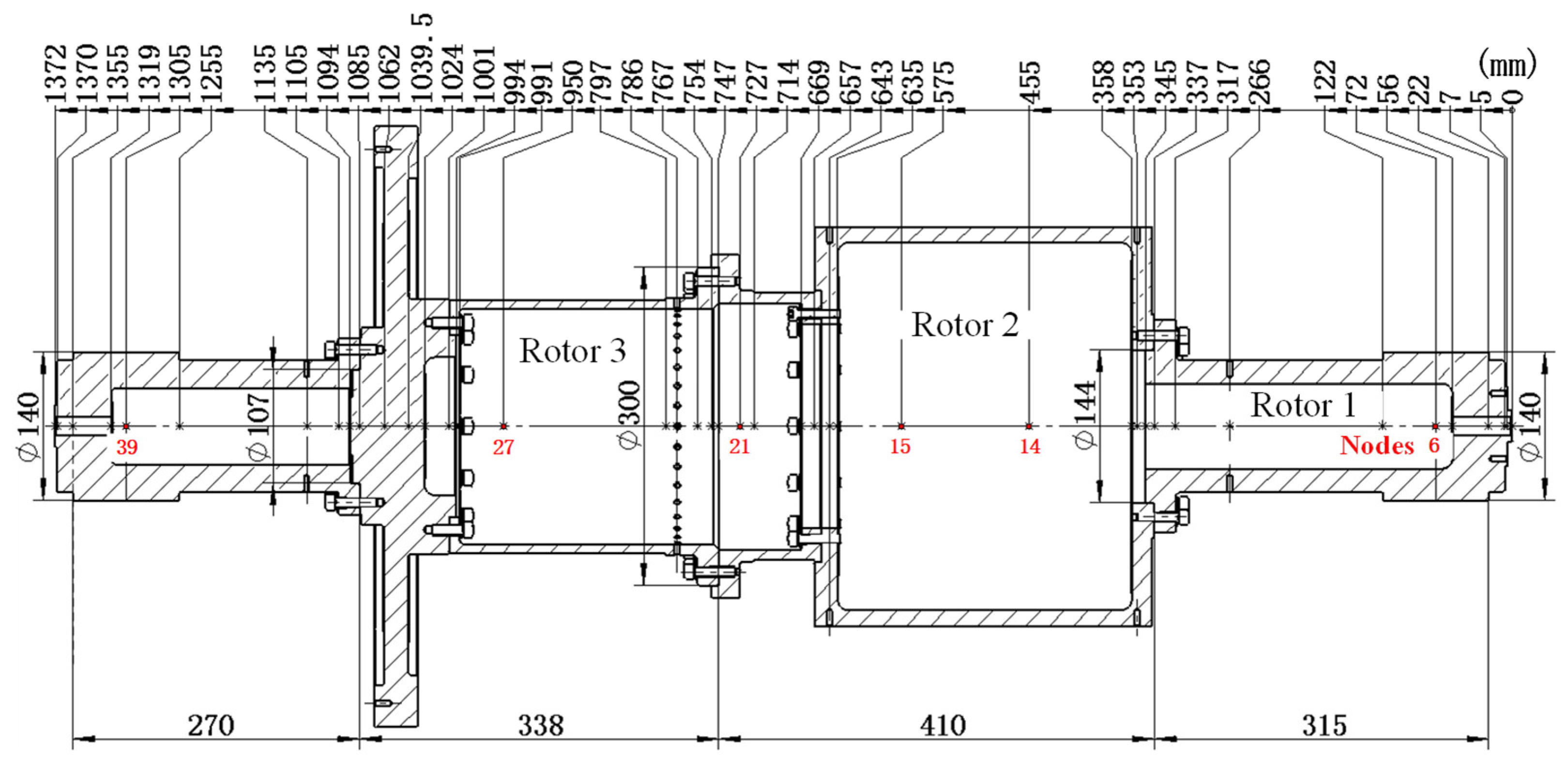
Figure 8 illustrates the key dimensions and node division of the finite element model for a four-stage assembled rotor. The detailed dimensional parameters of each shaft element are provided in

Table A1. Dimensional parameters of each shaft element.

Element No.	Ln (mm)	Dn (mm)	wn (mm)
1	5	30	17.5
2	2	75	17.5
3	15	124	17.5
4	34	140	17.5
5	16	140	80
6	50	140	80
7	144	124	80
8	51	124	80
9	20	200	80
10	8	376	80
11	8	376	144
12	5	376	144
13	97	376	346
14	120	376	346
15	60	376	346
16	8	376	192
17	14	376	192
18	12	252	192
19	45	252	232
20	13	256	232
21	20	324	232
22	7	324	222
23	13	300	222
24	19	242	222
25	11	242	222
26	153	238	222
27	41	238	222
28	3	238	171
29	7	238	130
30	23	240	130
31	15.5	240	0
32	22.5	566	0
33	23	186	0
34	9	166	0
35	11	166	72

of Appendix A. This rotor is a simplified 1:1 scale model of a real aero-engine high-pressure rotor system, scaled according to its dimensions, mass, and inertia. It is assembled step-by-step from four components: a front axle (Rotor 1), a compressor (Rotor 2), a high-pressure turbine (Rotor 3), and a rear axle (Rotor 4). The rotor material is defined as steel, with an elastic modulus of 210 GPa and a Poisson’s ratio of 0.3.

Its initial parameters are shown in

Table 1. Mass eccentricity errors for the individual rotor stages [25].

Rotor Stage No.	Unbalanced Mass Point Number	γjk (mm)	ljk (mm)	ujk (g)	φjk (°)
1	1	70	100	5	0
	2	62	244	5	0
2	1	188	16	5	0
	2	188	306	5	0
3	1	121	39	5	0
	2	261	324	5	0
4	1	62	50	5	0
	2	70	170	5	0

and

Table 2. Spigot eccentricity errors for the individual rotor stages [25].

Rotor Stage No.	cj (mm)	θj (°)	pj (mm)	hj (mm)	δj (°)	dj (mm)
1	0.02	0	0.02	315	0	72
2	0.02	90	0.02	410	90	150
3	0.02	180	0.02	338	180	53.5
4	0.02	270	0.02	270	270	70

. The vibration responses at six key positions (Nodes 6, 14, 15, 21, 27, and 39 in Figure 8) are selected to characterize the overall vibration level of the four-stage rotor at various rotational speeds. These nodes were chosen because they represent both the support boundaries (Nodes 6 and 39) and the key structural locations (disks and mid-spans) where vibration amplitudes are typically highest during critical speed traversal.

The assembly phases for each stage are defined as follows: The front axle is fixed by default, with its assembly angle ${\theta }_{z1}=0^{\circ }$. It is connected to the compressor using 12 evenly distributed screws. Therefore, after aligning the assembly screw holes of the compressor and the front axle, the selectable assembly angles for the compressor are ${\theta }_{z2}\in \{0^{\circ },{30}^{\circ },{60}^{\circ },{90}^{\circ },{120}^{\circ },{150}^{\circ },{180}^{\circ }\}$. The high-pressure turbine is connected to the compressor using 24 evenly distributed screws. After aligning their assembly screw holes, the selectable assembly angles for the high-pressure turbine are ${\theta }_{z3}\in \{0^{\circ },{15}^{\circ },{30}^{\circ },{45}^{\circ },{60}^{\circ },{75}^{\circ },{90}^{\circ },{105}^{\circ },{120}^{\circ },{135}^{\circ },{150}^{\circ },{165}^{\circ },{180}^{\circ }\}$. The rear axle is connected to the high-pressure turbine using 12 evenly distributed screws. Thus, after aligning their assembly screw holes, the selectable assembly angles for the rear axle, ${\theta }_{z4}$, are the same as those for ${\theta }_{z2}$.

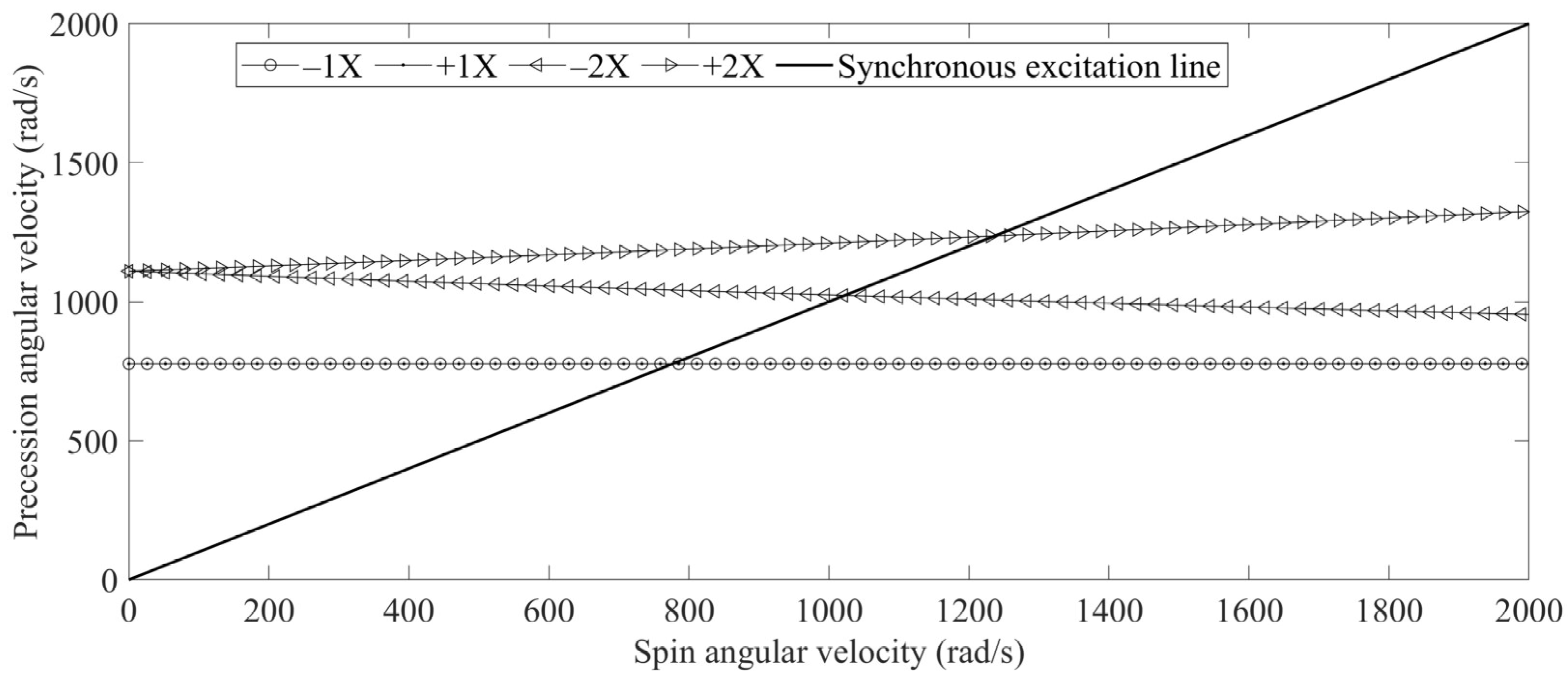
A Campbell diagram of the four-stage rotor system was constructed using MATLAB R2022b to identify its critical speeds, as presented in Figure 9. The analysis accounts for gyroscopic effects over a speed range of 0–15,000 rpm. The intersections of the forward whirl eigenfrequency curves with the 1× excitation line yield the first two critical speeds at 7421 rpm and 11,810 rpm, which correspond to the first and second bending modes. Based on the critical speeds obtained from the simulation, three objective functions are formulated:

• A function using solely the maximum displacement amplitude across the six nodes at the first critical speed: f₇₄₂₁(θ_z2, θ_z3, θ_z4).
• A function using solely the maximum displacement amplitude across the six nodes at the second critical speed: f_11,810(θ_z2, θ_z3, θ_z4).
• A normalized objective function considering both the first and second critical speeds—the normalized maximum displacement amplitude across the six nodes: F(θ_z2, θ_z3, θ_z4) (Equation (9)).

$$F({\theta }_{z2},{\theta }_{z3},{\theta }_{z4})={\left[{\displaystyle \frac{f_{7421}({\theta }_{z2},{\theta }_{z3},{\theta }_{z4})-\nabla f_{7421}}{\nabla f_{7421}}}\right]}^2+{\left[{\displaystyle \frac{f_{11810}({\theta }_{z2},{\theta }_{z3},{\theta }_{z4})-\nabla f_{11810}}{\nabla f_{11810}}}\right]}^2.$$

(31)

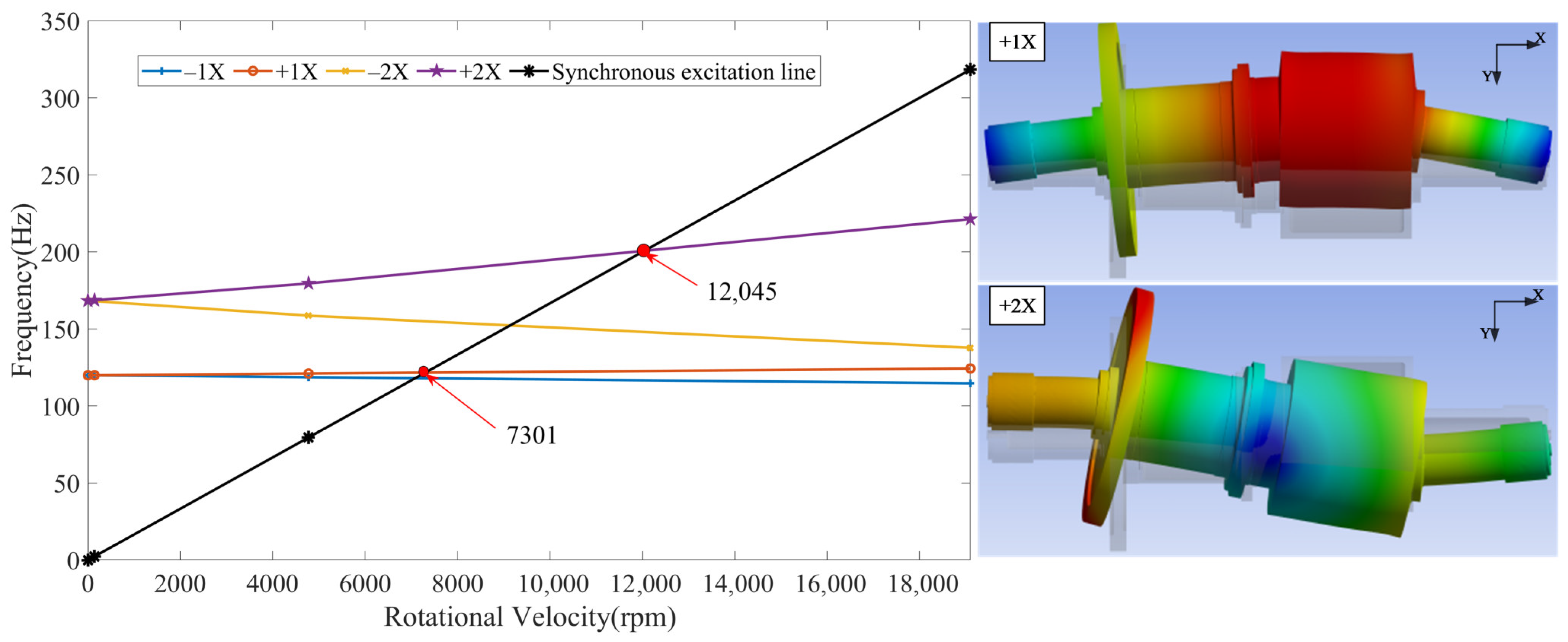
To further validate the critical speeds obtained from the MATLAB-based finite element beam model, a separate three-dimensional solid model of the four-stage rotor was reconstructed in ANSYS Workbench 2022R2. Modal analysis accounting for gyroscopic effects was performed over the same rotational speed range. The resulting Campbell diagram is presented in Figure 10. The intersections of the forward whirl frequency curves with the 1× excitation line yield the first two critical speeds at 7301 rpm and 12,045 rpm, corresponding to the first and second bending modes, respectively.

The critical speeds obtained from the ANSYS simulation show good agreement with those from the MATLAB numerical calculation, with relative differences of approximately 1.6% and 1.9% for the first and second critical speeds. This consistency confirms the reliability of the finite element models used in this study. The slight discrepancies can be attributed to the different modeling approaches—beam elements in MATLAB versus 3D solid elements in ANSYS Workbench—as well as variations in meshing strategies and element formulations.

Using the optimal, worst, and default assembly angle sequences (i.e., {θ_z2 = 0°, θ_z3 = 0°, θ_z4 = 0°}) obtained from the optimization based on each of the three objective functions above, the corresponding maximum displacement amplitudes across the six nodes for the four-stage rotor are compared at the following rotational speeds: 1000 rpm, 3000 rpm, 5000 rpm, 7421 rpm, 9000 rpm, 11,810 rpm, and 14,000 rpm.

It should be noted that the assembly angles are discrete variables rather than continuous ones. This is because the rotors are connected by evenly distributed screws (12 or 24 screws), so the actual assembly phases are limited to discrete angular increments (e.g., 30° for 12-screw connections, 15° for 24-screw connections). Therefore, interpolation is not required for trajectory planning, as the optimization directly searches over the discrete feasible space. The initialization and mutation steps in the genetic algorithm (see Section 2.8) also enforce that all candidate solutions remain within these discrete sets.

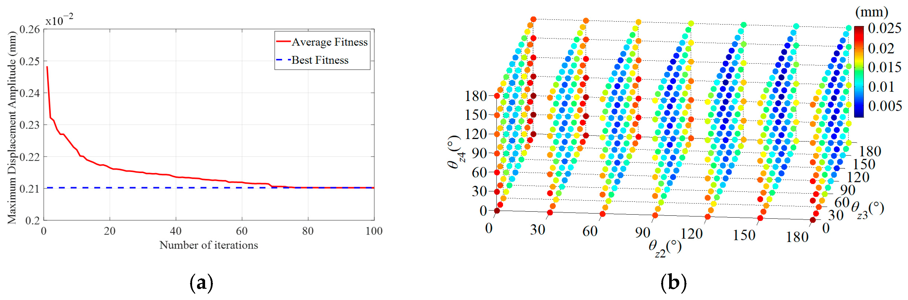
Figure 11a shows the convergence curve of the genetic optimization using f₇₄₂₁(θ_z2, θ_z3, θ_z4) as the objective function. The optimal fitness value, which corresponds to the maximum displacement amplitude across the six nodes at the first critical speed, is 0.0021 mm. The corresponding optimal assembly angle sequence is {θ_z2 = 150°, θ_z3 = 105°, θ_z4 = 120°}. At this optimal sequence, the maximum displacement amplitude across the six nodes at the second critical speed is 0.0129 mm.

As shown in Figure 11b, the exhaustive angle traversal method was used to calculate the value of f₇₄₂₁(θ_z2, θ_z3, θ_z4)—the six-node maximum displacement amplitude—for all possible assembly angle sequences. This serves two purposes: firstly, to verify the accuracy of the genetic optimization results; and secondly, to identify the worst assembly angle sequence, which is {θ_z2 = 0°, θ_z3 = 180°, θ_z4 = 30°}. For this worst sequence, the maximum displacement amplitudes at the first and second critical speeds increase to 0.0258 mm and 0.0230 mm, respectively.

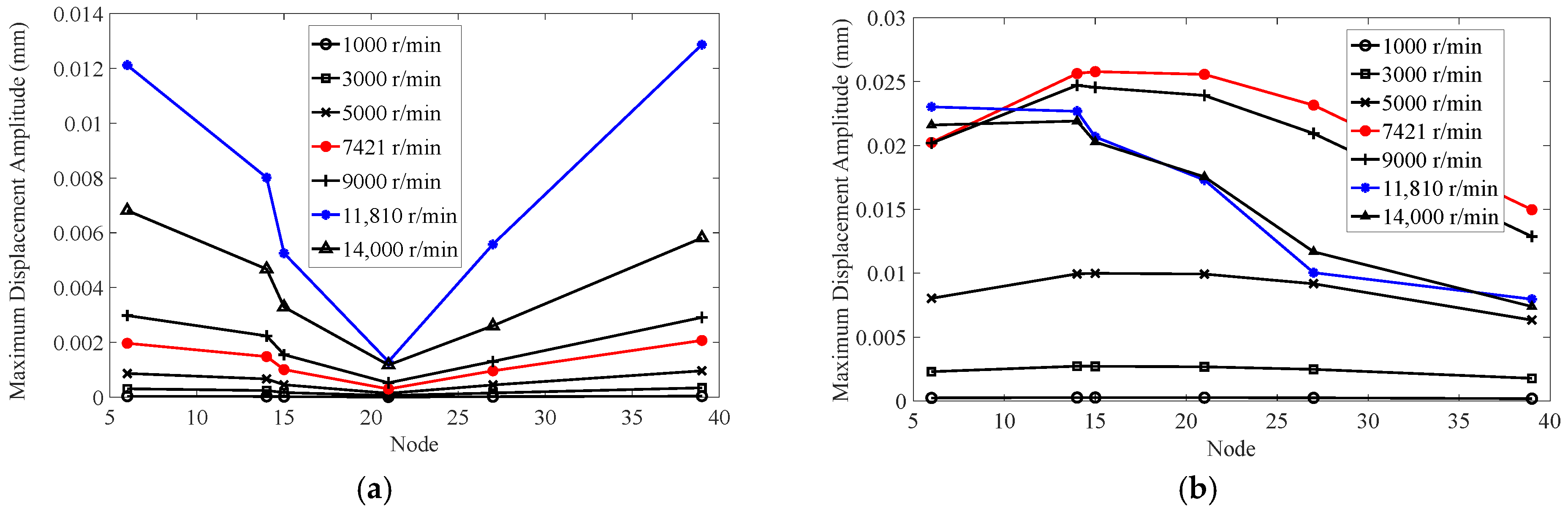
Figure 12 presents the maximum displacement amplitudes across the six nodes at various preset rotational speeds for both the optimal and the worst assembly angle sequences when f₇₄₂₁(θ_z2, θ_z3, θ_z4) is used as the objective function.

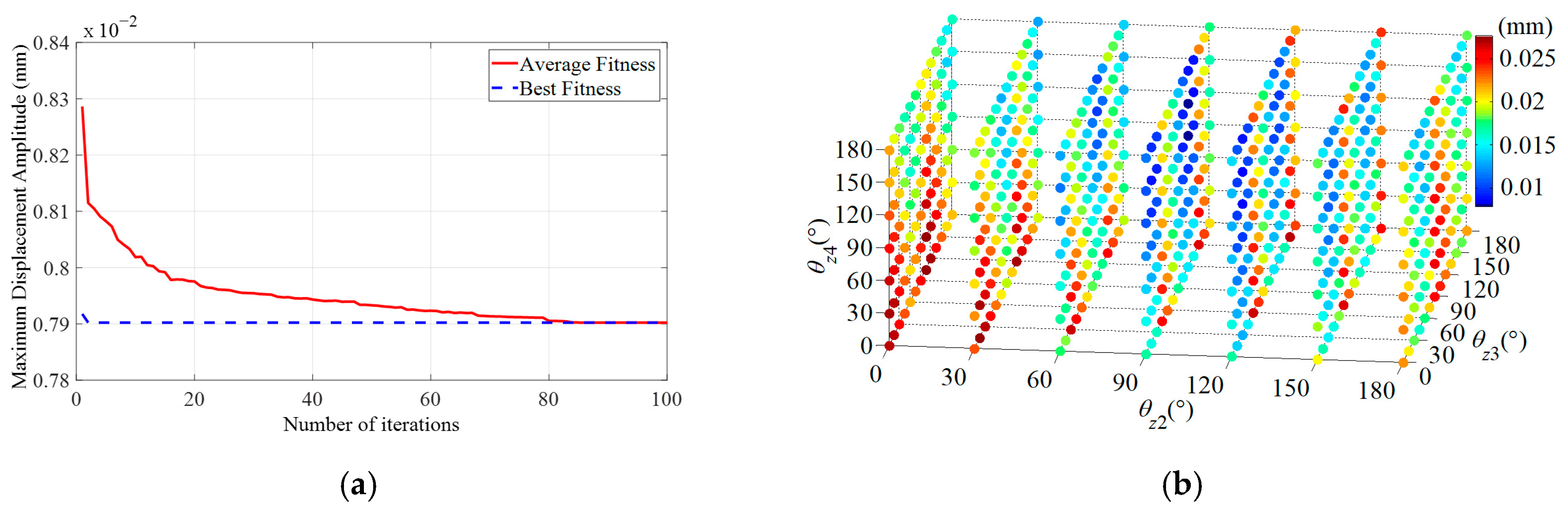
Figure 13a shows the convergence curve of the genetic optimization using f_11,810(θ_z2, θ_z3, θ_z4) as the objective function. The optimal fitness value, which corresponds to the maximum displacement amplitude across the six nodes at the second critical speed, is 0.007 9 mm. The corresponding optimal assembly angle sequence is {θ_z2 = 90°, θ_z3 = 120°, θ_z4 = 150°}. For this sequence, the maximum displacement amplitude at the first critical speed is 0.004 1 mm. As shown in Figure 13b, the exhaustive angle traversal method was used to calculate f_11,810(θ_z2, θ_z3, θ_z4)—the six-node maximum displacement amplitude—for all possible assembly angle sequences, identifying the worst sequence as {θ_z2 = 0°, θ_z3 = 105°, θ_z4 = 0°}. For this worst sequence, the maximum displacement amplitudes at the first and second critical speeds increase to 0.0191 mm and 0.0276 mm, respectively.

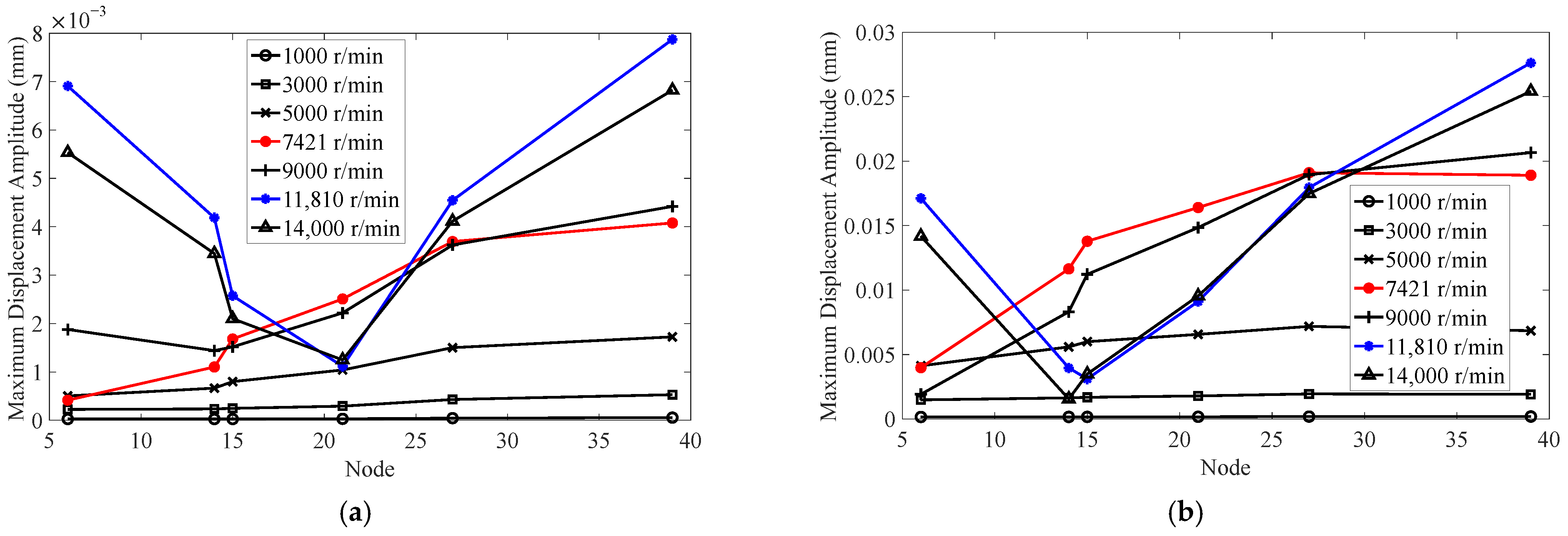
Figure 14 presents the maximum displacement amplitudes across the six nodes at various preset rotational speeds for both the optimal and the worst assembly angle sequences when f_11,810(θ_z2, θ_z3, θ_z4) is used as the objective function.

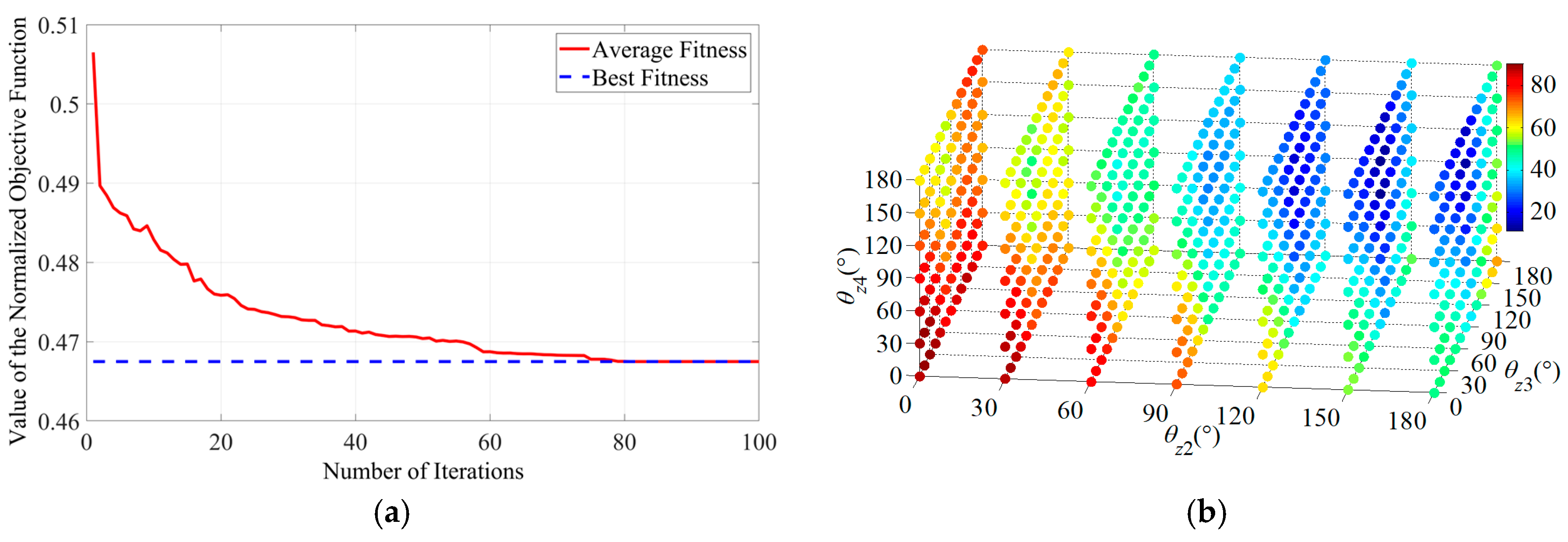
Figure 15a shows the convergence curve of the genetic optimization using the normalized objective function F(θ_z2, θ_z3, θ_z4). The corresponding optimal assembly angle sequence for the best fitness is {θ_z2 = 150°, θ_z3 = 180°, θ_z4 = 150°}. For this optimal sequence, the maximum displacement amplitudes across the six nodes at the first and second critical speeds are 0.0035 mm and 0.0091 mm, respectively. As shown in Figure 15b, the exhaustive angle traversal method was used to evaluate F(θ_z2, θ_z3, θ_z4)—the six-node maximum displacement amplitude—for all possible assembly angle sequences. This process identified the worst assembly angle sequence as {θ_z2 = 0°, θ_z3 = 30°, θ_z4 = 0°}. For this worst sequence, the maximum displacement amplitudes at the first and second critical speeds increase to 0.0214 mm and 0.0261 mm, respectively.

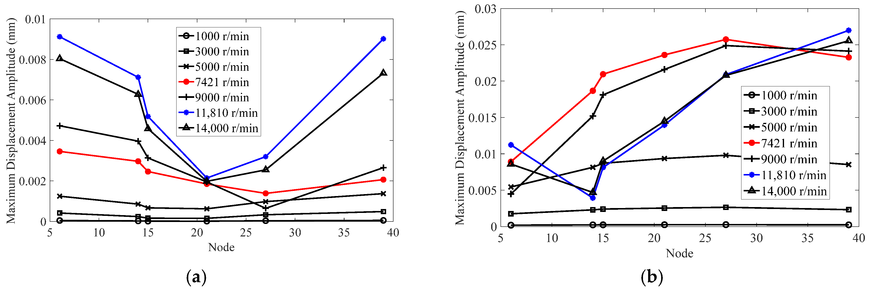
Figure 16 presents the maximum displacement amplitudes across the six nodes at various preset rotational speeds for both the optimal and the worst assembly angle sequences when the normalized objective function F(θ_z2, θ_z3, θ_z4) is employed.

The convergence characteristics of the genetic algorithm are consistent across all three objective functions. From the convergence curves presented in Figure 11a, Figure 13a and Figure 15a the following observations can be made:

• The algorithm converges rapidly within the first 20–30 generations, demonstrating efficient exploration of the search space.
• The best fitness value stabilizes after approximately 80 generations, indicating that convergence is achieved well before the maximum iteration limit of 100 generations.
• No significant oscillations are observed in the best fitness curves, confirming the stability of the optimization process.

These convergence characteristics demonstrate the reliability of the genetic algorithm in identifying optimal assembly angle sequences for the four-stage rotor system. To ensure the global optimality of the obtained assembly angle sequences, multiple validation strategies were employed.

First, the exhaustive search (angle traversal) was performed for each objective function, as shown in Figure 11b, Figure 13b and Figure 15b. The total number of feasible assembly angle combinations for the four-stage rotor is $7\times 13\times 7=637$. In all cases, the optimal solutions identified by the genetic algorithm matched the results of the exhaustive search, confirming that the algorithm successfully identified the global optimum.

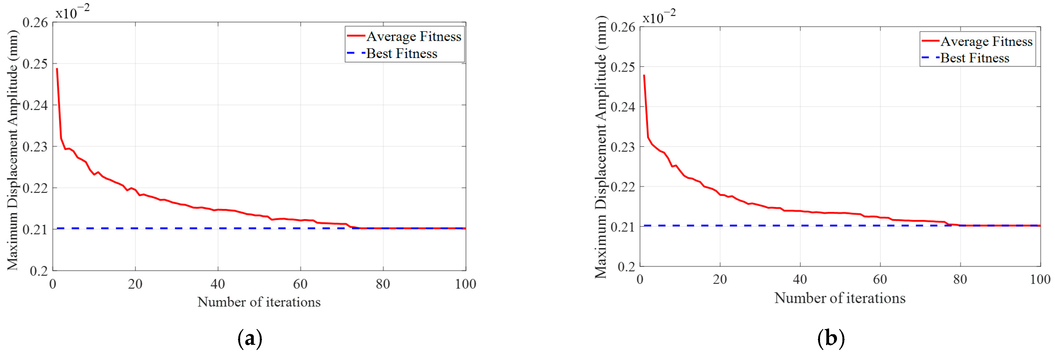
Second, multiple independent runs were conducted with different random seeds to verify robustness. Figure 11a shows the convergence curve of the first independent run using $f_{7421}({\theta }_{z2},{\theta }_{z3},{\theta }_{z4})$ as the objective function, where the best fitness converged to 0.0021 mm after approximately 80 iterations. The convergence curves of the second and third independent runs are presented in Figure 17a,b, respectively. The following observations can be made from these figures:

• In all three runs, the best fitness value converges to 0.0021 mm, which is identical to the optimal value identified by the exhaustive search (see Figure 11b).
• The average fitness also shows consistent convergence behavior, with the population mean approaching the optimal value as iterations progress.
• The convergence speed and stability are comparable across all runs, with no significant oscillations or premature convergence observed.

These results demonstrate that the genetic algorithm, combined with the strategies of large population size (1000 individuals), adaptive mutation, and elite preservation with worst replacement, consistently identifies the global optimum regardless of the initial population. The close agreement between the optimal solutions obtained from multiple independent runs and the exhaustive search further validates that the algorithm does not become trapped in local optima.

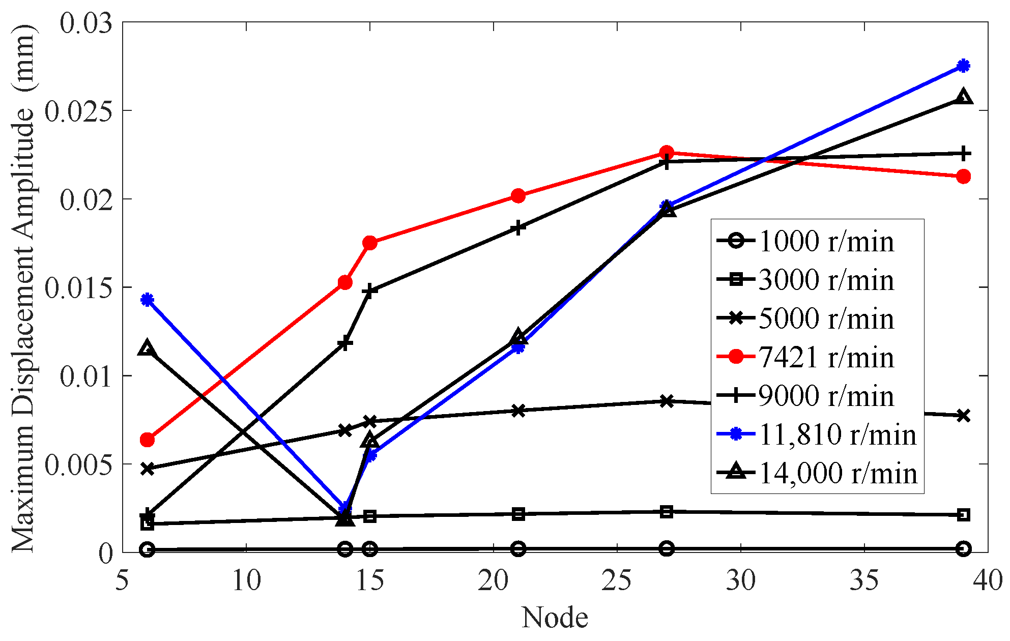
As shown in Figure 18, the maximum displacement amplitudes across the six nodes of the four-stage rotor at the preset rotational speeds under the default assembly angle sequence are presented. Under this condition, the maximum displacement amplitudes at the first and second critical speeds are 0.0257 mm and 0.0270 mm, respectively.

Table 3. Maximum displacement amplitude across the six nodes under different assembly states obtained using the three objective functions.

Rotational Speed (rpm)	Default Assembly (×10−4 mm)	min {f7421(θz2, θz3, θz4)} (×10−4 mm)		min {f11,810(θz2, θz3, θz4)} (×10−4 mm)		min {F(θz2, θz3, θz4)} (×10−4 mm)
		Optimal Assembly	Worst Assembly	Optimal Assembly	Worst Assembly	Optimal Assembly	Worst Assembly
1000	2	0	3	1	2	1	3
3000	23	3	27	5	19	5	26
5000	86	10	100	17	72	14	98
7421	226	21	258	41	191	35	257
9000	226	30	247	44	207	47	249
11,810	275	129	230	79	276	91	270
14,000	257	68	219	68	254	80	255

presents the maximum displacement amplitudes across the six nodes at various preset rotational speeds under different assembly states, obtained using the three objective functions described above. The following observations can be drawn from Table 3:

• Compared with the default assembly angle sequence, the optimal sequence obtained using f₇₄₂₁(θ_z2, θ_z3, θ_z4) as the objective function reduces the maximum displacement amplitudes at the first and second critical speeds by 90.7% and 53.1%, respectively. Compared with the worst assembly angle sequence, the reductions are 91.9% and 43.9%, respectively.
• Compared with the default assembly angle sequence, the optimal sequence obtained using f_11,810(θ_z2, θ_z3, θ_z4) as the objective function reduces the maximum displacement amplitudes at the first and second critical speeds by 81.9% and 71.3%, respectively. Compared with the worst assembly angle sequence, the reductions are 78.5% and 71.4%, respectively.
• Compared with the default assembly angle sequence, the optimal sequence obtained using the normalized objective function F(θ_z2, θ_z3, θ_z4) reduces the maximum displacement amplitudes at the first and second critical speeds by 84.5% and 66.9%, respectively. Compared with the worst assembly angle sequence, the reductions are 86.4% and 66.3%, respectively.
• By comparing the range of the vertical axis (displacement amplitude) in Figure 12a versus Figure 12b and Figure 14a versus Figure 14b and Figure 16a versus Figure 16b, it is evident that the optimal assembly angle sequences derived from all three objective functions lead to an overall reduction in the displacement amplitudes across the six nodes for the four-stage rotor at all investigated rotational speeds.

The results above lead to the following conclusions:

• Using f₇₄₂₁(θ_z2, θ_z3, θ_z4) as the objective function yields the minimum vibration response at the first critical speed. While it also suppresses the vibration at the second critical speed, the achieved second-order response is 63.3% higher compared to when f_11,810(θ_z2, θ_z3, θ_z4) is used as the objective function.
• Using f_11,810(θ_z2, θ_z3, θ_z4) as the objective function yields the minimum vibration response at the second critical speed. While it also suppresses the vibration at the first critical speed, the achieved first-order response is 66.7% higher compared to when f₇₄₂₁(θ_z2, θ_z3, θ_z4) is used as the objective function.
• Using the normalized objective function F(θ_z2, θ_z3, θ_z4) does not achieve the absolute minimum vibration response at either individual critical speed. However, it balances the suppression effects of the single objectives. This is the role of the normalized function: to enable the rotor to traverse both the first and second critical speeds smoothly. If there is a need to prioritize the suppression of vibration at a specific critical speed, a weighting factor can be introduced into Equation (29). An appropriate factor can then be selected through trial calculations to achieve the desired emphasis.
• Employing the genetic algorithm for the global optimization of the four-stage rotor’s assembly angles requires only approximately 80 iterations to converge to the optimal sequence. This represents a significant time saving compared to the exhaustive search over all possible phase sequences (7 × 13 × 7 = 637 calculations). Furthermore, as the number of rotor stages and assembly bolt holes increases, the computational cost of the exhaustive method grows exponentially.

3.2. Comparative Analysis of Vibration Reduction Effectiveness with Existing Objective Functions

The primary distinction among existing methods for optimizing the assembly angles of multi-stage rotors lies in their objective functions, which can be categorized as follows:

• Maximum geometric eccentricity of the multi-stage rotor [10,11,12,13]—Expressed using the parameters of this study’s model as

  $$C\left({{\theta }_z}_2,{{\theta }_z}_3,{{\theta }_z}_4\right)=\max \left\{c_1,c_2,\dots ,c_j\right\}.$$

  (32)
• Comprehensive unbalance of the multi-stage rotor [18]—Expressed using the parameters of this study’s model as

  $$U\left({{\theta }_z}_2,{{\theta }_z}_3,{{\theta }_z}_4\right)=\max \left\{U_{\mathrm{A}},U_{\mathrm{B}}\right\}.$$

  (33)
• Dual-objective evaluation function [17,19] for C(θ_z2, θ_z3, θ_z4) and U(θ_z2, θ_z3, θ_z4)—Expressed using the parameters of this study’s model as

  $$C\&U\left({{\theta }_z}_2,{{\theta }_z}_3,{{\theta }_z}_4\right)=\max \left\{{\left[{\displaystyle \frac{C-\nabla C}{\nabla C}}\right]}^2+{\left[{\displaystyle \frac{U-\nabla U}{\nabla U}}\right]}^2\right\}$$

  (34)

  where ∇C is the minimum value of the maximum geometric eccentricity C obtained from single-objective optimization, and ∇U is the minimum value of the comprehensive unbalance U obtained from single-objective optimization.
• Vibration response at the operational speed [20,21,22,23]—Since the four-stage rotor used in this study is a simplified model of a certain type of engine’s high-pressure rotor, its actual operational speed is above the second critical speed, approximately 17,000 rpm. Therefore, it can be expressed using this study’s parameters as f_17,000(θ_z2, θ_z3, θ_z4).

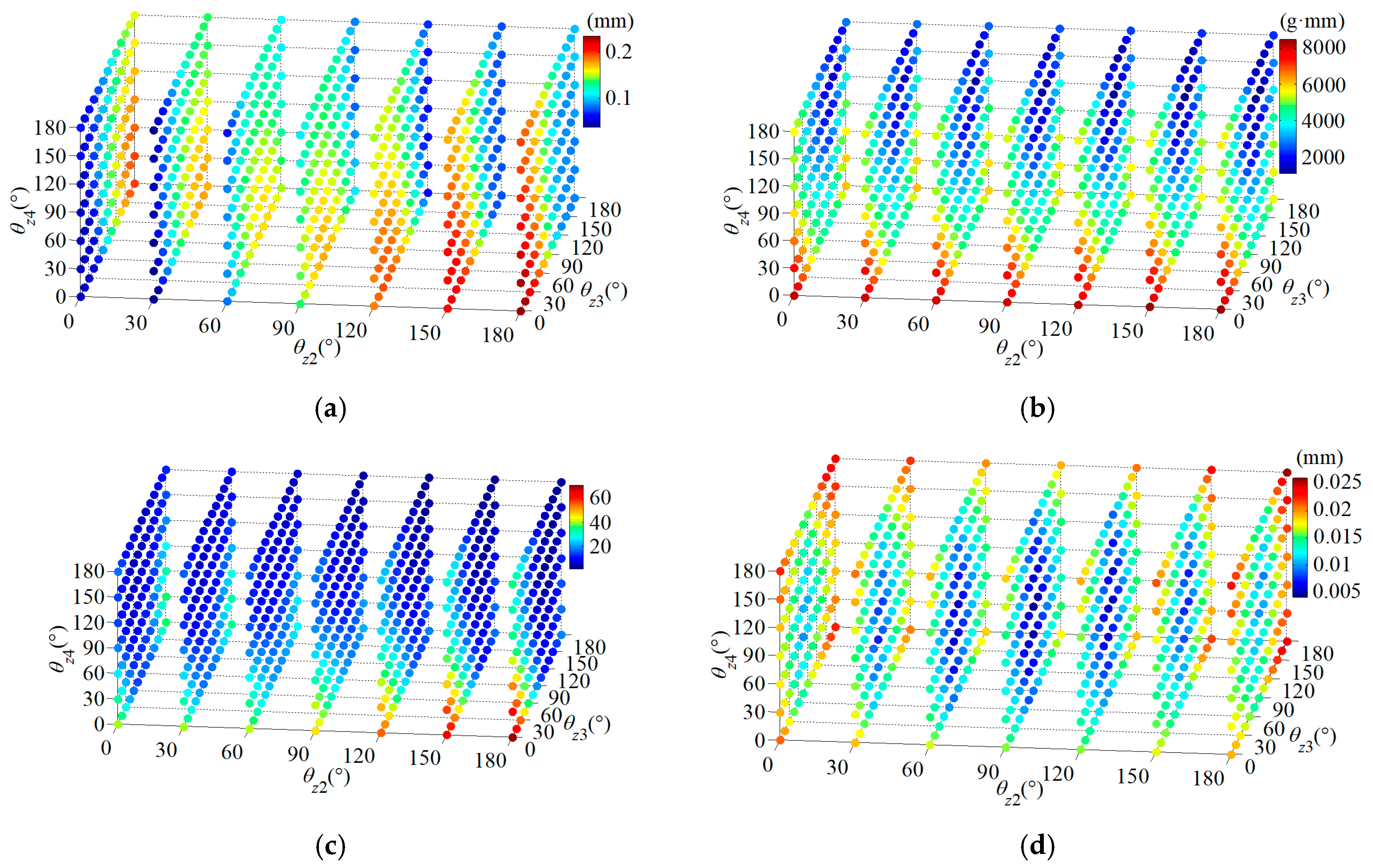
Figure 19 shows the exhaustive search results for the four aforementioned objective functions.

Table 4. Maximum displacement amplitude across the six nodes under the optimal assembly states obtained using the four optimization objectives.

Objective Function	Optimal Assembly Angle Sequence	f7421(θz2, θz3, θz4) (mm)	f11,810(θz2, θz3, θz4) (mm)
C (θz2, θz3, θz4)	θz2 = 30°, θz3 = 0°, θz4 = 0°	0.0236	0.0267
U (θz2, θz3, θz4)	θz2 = 150°, θz3 = 135°, θz4 = 150°	0.0064	0.0112
C&U (θz2, θz3, θz4)	θz2 = 150°, θz3 = 150°, θz4 = 150°	0.0088	0.0123
f17,000(θz2, θz3, θz4)	θz2 = 90°, θz3 = 90°, θz4 = 90°	0.0063	0.0132

lists the optimal assembly angle sequence corresponding to each objective function, along with the resulting maximum displacement amplitudes across the six nodes at the first and second critical speeds. The following observations can be made:

• Compared to the default assembly angle sequence, the optimal sequence obtained using the maximum geometric eccentricity C (θ_z2, θ_z3, θ_z4) as the objective function reduces the maximum displacement amplitude at the second critical speed by a mere 0.03%. Conversely, the amplitude at the first critical speed increases by 4.4%.
• Compared to the default assembly angle sequence, the optimal sequence obtained using the comprehensive unbalance U (θ_z2, θ_z3, θ_z4) as the objective function reduces the maximum displacement amplitudes at the first and second critical speeds by 70.4% and 59.3%, respectively.
• Compared to the default assembly angle sequence, the optimal sequence obtained using the dual-objective function C&U (θ_z2, θ_z3, θ_z4) as the objective function reduces the maximum displacement amplitudes at the first and second critical speeds by 61.1% and 55.3%, respectively.
• Compared to the default assembly angle sequence, the optimal sequence obtained using the operational speed vibration response f_17,000(θ_z2, θ_z3, θ_z4) as the objective function reduces the maximum displacement amplitudes at the first and second critical speeds by 72.1% and 52.0%, respectively.

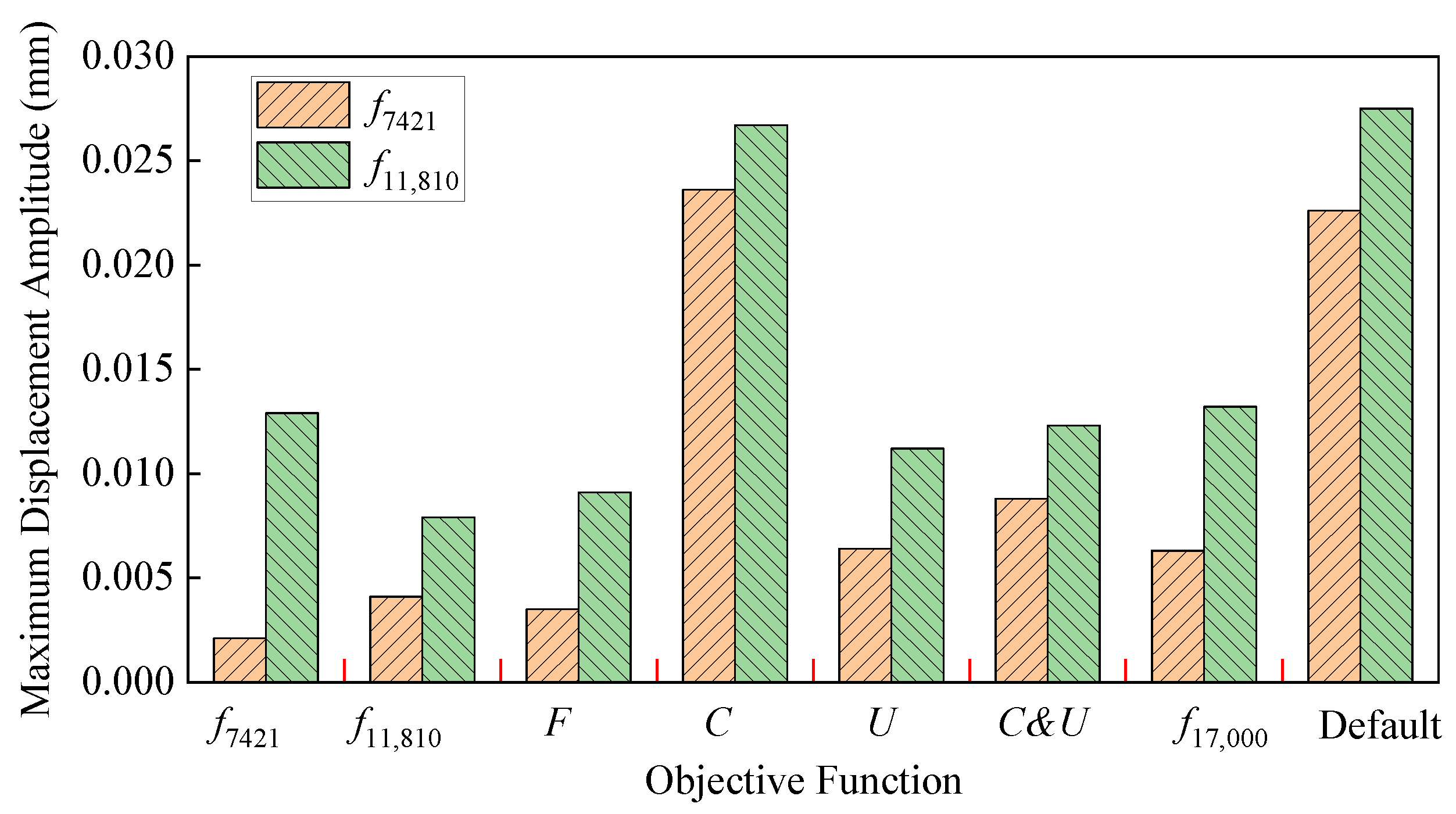
Integrating the maximum displacement amplitudes across the six nodes at the first and second critical speeds for the optimal assembly angle sequences obtained from the three objective functions introduced in Section 3.1 of this study, along with those for the default assembly angle sequence, a bar chart is plotted (Figure 20). This provides an intuitive visualization, revealing that:

• Regarding the suppression of vibration at the first critical speed, the optimal sequences derived from the different objective functions are ranked from most to least effective as follows: f₇₄₂₁, F, f_11,810, f_17,000, U, C&U, Default, C.
• Regarding the suppression of vibration at the second critical speed, the ranking is: f_11,810, F, U, C&U, f_17,000, f₇₄₂₁, C, Default.

The results indicate that, compared to the objective functions constructed in existing studies, the normalized objective function for multi-speed vibration response F(θ_z2, θ_z3, θ_z4) proposed in this work provides superior comprehensive suppression effectiveness on the vibration response across the six nodes of the four-stage rotor at its respective critical speeds.

4. Experimental Verification

4.1. Experimental Setup

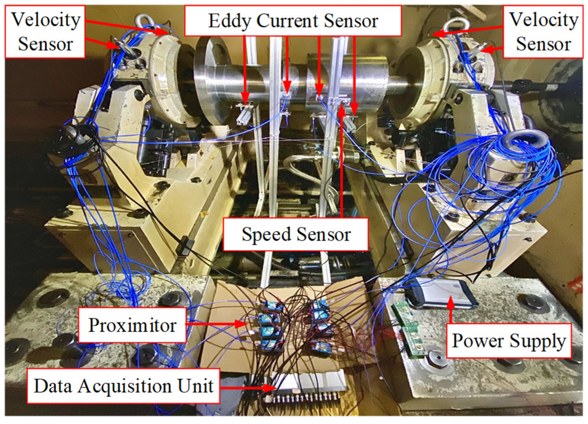
The experimental rotor used in simulation serves as the test subject, with its geometric and mass characteristic parameters for each single-stage rotor already provided by measurement in Reference [29]. As shown in Figure 21, the experimental setup employs a Shanghai XINKE DG10-6 vacuum high-speed balancing machine as the drive platform (0–15,000 rpm), with the four-stage assembled rotor horizontally mounted and its front and rear journals supported by pendulum-type bearing housings. The overall rotor length from the front-end face to the rear-end face is 1372 mm, with a bearing span of 1233 mm between the front and rear journal centers. Both journals have a diameter of 140 mm and a surface roughness of Ra ≤ 0.8 μm to ensure consistent support conditions. All vibration sensors are positioned according to the six node locations defined in the finite element model (Nodes 6, 14, 15, 21, 27, and 39), with axial distances measured from the front end face: Node 6 (front bearing) at 72 mm, Node 14 (front compressor section) at 455 mm, Node 15 (rear compressor section) at 575 mm, Node 21 (compressor outlet) at 727 mm, Node 27 (high-pressure turbine) at 950 mm, and Node 39 (rear bearing) at 1305 mm. Eddy current sensors (5 mm probe diameter, 0–2 mm range, linearity error < 1%) and velocity sensors (20 mV/mm/s sensitivity, 10–1000 Hz frequency response) are used accordingly. The rotor is driven by a variable-frequency motor through a flexible coupling (outer diameter 100 mm, length 300 mm) and a flexible adapter shaft (length 250 mm, outer diameter 140 mm), designed to minimize transmission of axial and bending moments.

• Under the default assembly angle sequence, a run-up test from 0 to 15,000 rpm was conducted on the four-stage rotor using the high-speed balancing machine to identify and calibrate its actual first and second critical speeds.
• Based on the seven vibration response objective functions compared in Section 3.2 (three proposed in this study and four from existing studies), an additional function F′(θ_z2, θ_z3, θ_z4) was considered. This function is calculated using the dynamic model without considering flexible dynamic deflection from refs. [20,21,22]. Following the eight optimal assembly angle sequences derived from these eight objective functions, the four-stage rotor was assembled eight separate times. After each assembly, a run-up test was performed.

4.2. Experimental Results

4.2.1. Preprocessing of Experimental Results

In our previous work, we analyzed the time-frequency characteristics of the vibration response of the multi-stage rotor under spigot eccentricity excitation and mass eccentricity excitation. The excitation from these two sources only manifests at the fundamental frequency. Therefore, a band-pass filtering process was applied to the measurement data from all sensors, extracting only the fundamental frequency components. This process filters out the DC component, as well as high- and low-frequency signals that may arise from faults such as bearing misalignment, drive misalignment, or oil film instability.

4.2.2. Calibration of the Critical Speeds for the Four-Stage Rotor

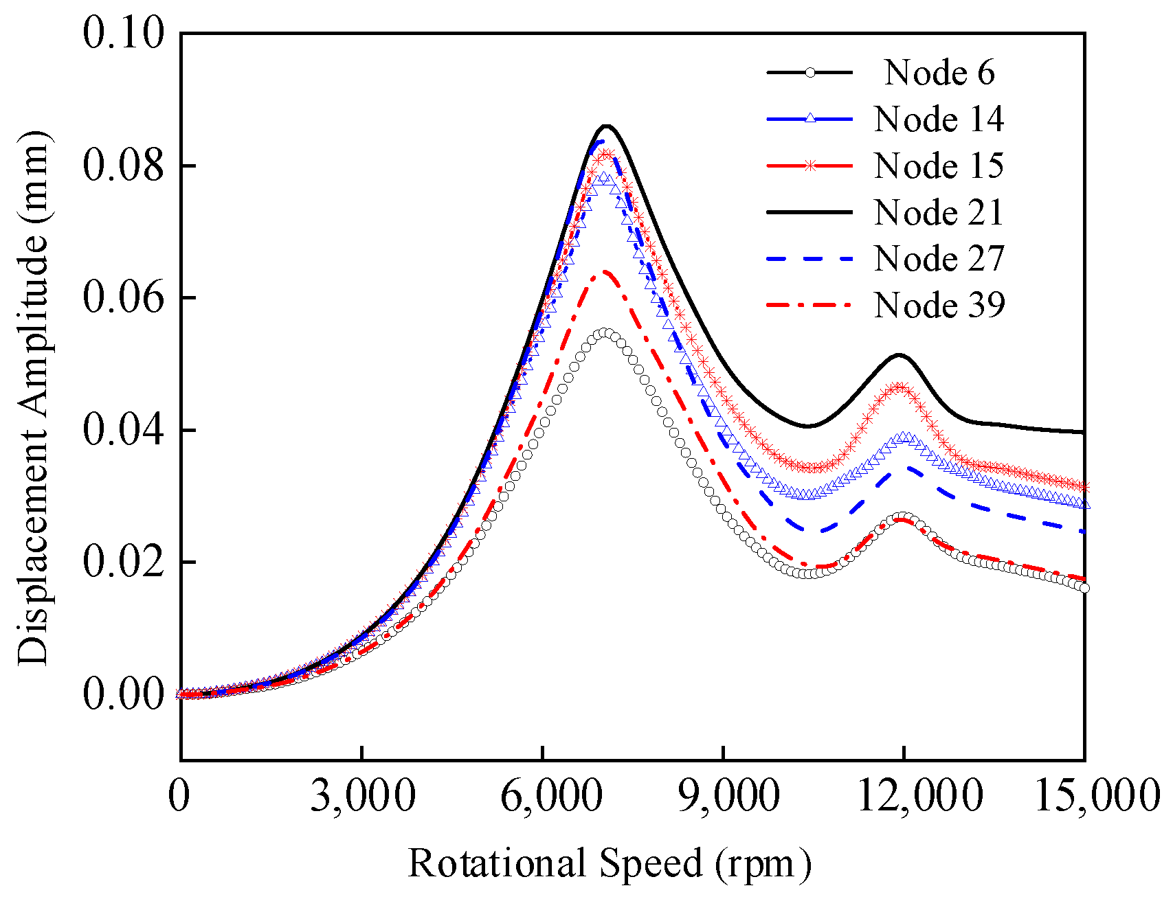
To validate the numerical models, the critical speeds obtained from experiments and simulations are compared. The experimentally measured first and second critical speeds under the default assembly angle sequence are 7000 rpm and 12,000 rpm, respectively, as shown in Figure 22. Two independent numerical simulations were performed: a MATLAB-based finite element beam model and an ANSYS Workbench 3D solid model. The MATLAB calculations yielded critical speeds of 7421 rpm and 11,810 rpm, while the ANSYS simulations yielded 7301 rpm and 12,045 rpm. The experimental results show good agreement with both numerical simulations, with deviations ranging from 0.4% to 6.0%. These slight discrepancies can be attributed to idealized support stiffness assumptions in the models, manufacturing tolerances in the experimental rotor, and measurement uncertainties. Overall, the consistent trend between the experimental and numerical results confirms the reliability of the finite element models used in this study.

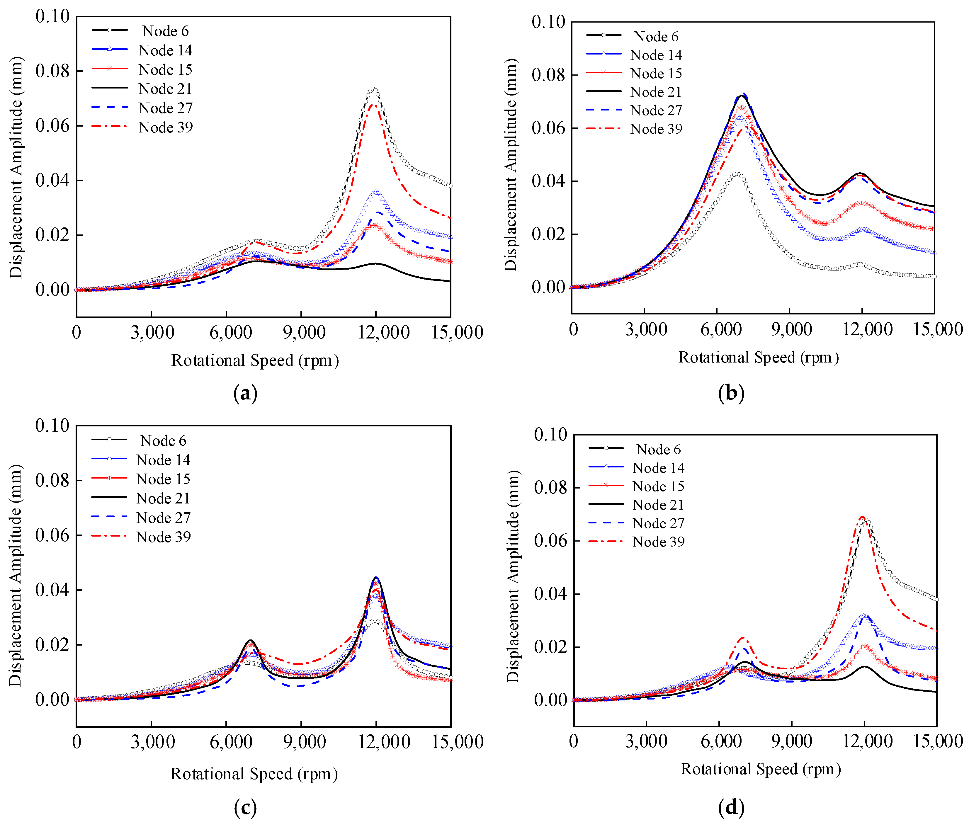
The first experimental step involved testing the four-stage rotor under the default assembly angle sequence. Figure 14 shows the experimentally measured run-up curves at the fundamental frequency for the displacement amplitudes across the six nodes from 0 to 15,000 rpm. Distinct peaks in the displacement amplitudes of all six nodes are observable near 7000 rpm and 12,000 rpm, indicating the locations of the first and second critical speeds, respectively.

4.2.3. Test Comparison of Vibration Reduction Effectiveness with Existing Objective Functions

In the second step of the experiment and considering the speed range and safety factors of the balancing machine, the rotational speed for the operational vibration response objective function was set to 14,000 rpm. Utilizing the multi-stage rotor assembly angle optimization algorithm established in Section 3.2, eight optimal assembly angle sequences were solved for, corresponding to the following eight objective functions: f₇₀₀₀(θ_z2, θ_z3, θ_z4), f_12,000(θ_z2, θ_z3, θ_z4), F(θ_z2, θ_z3, θ_z4), F′(θ_z2, θ_z3, θ_z4), C(θ_z2, θ_z3, θ_z4), U(θ_z2, θ_z3, θ_z4), C&U(θ_z2, θ_z3, θ_z4), f_14,000(θ_z2, θ_z3, θ_z4).

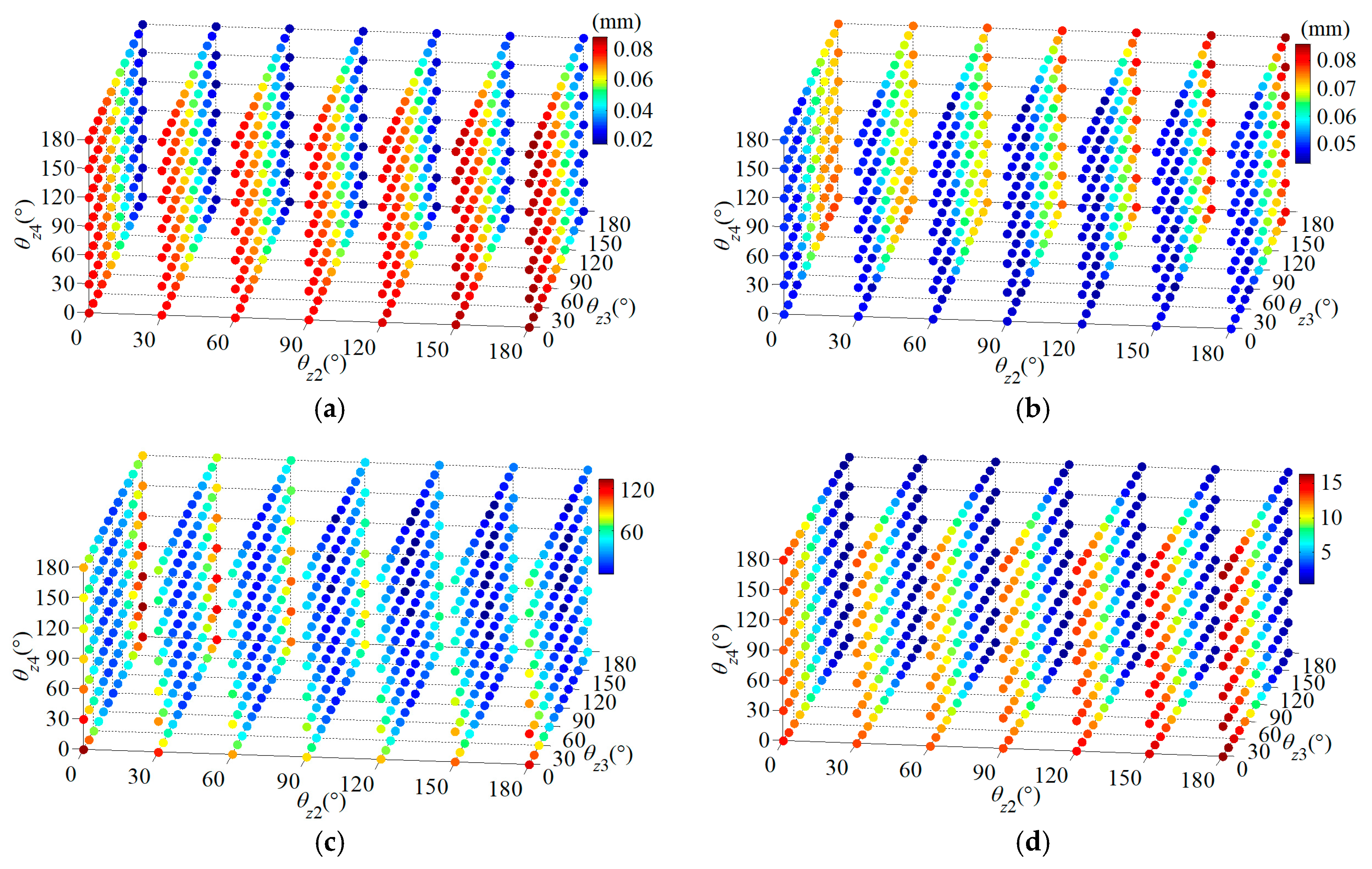
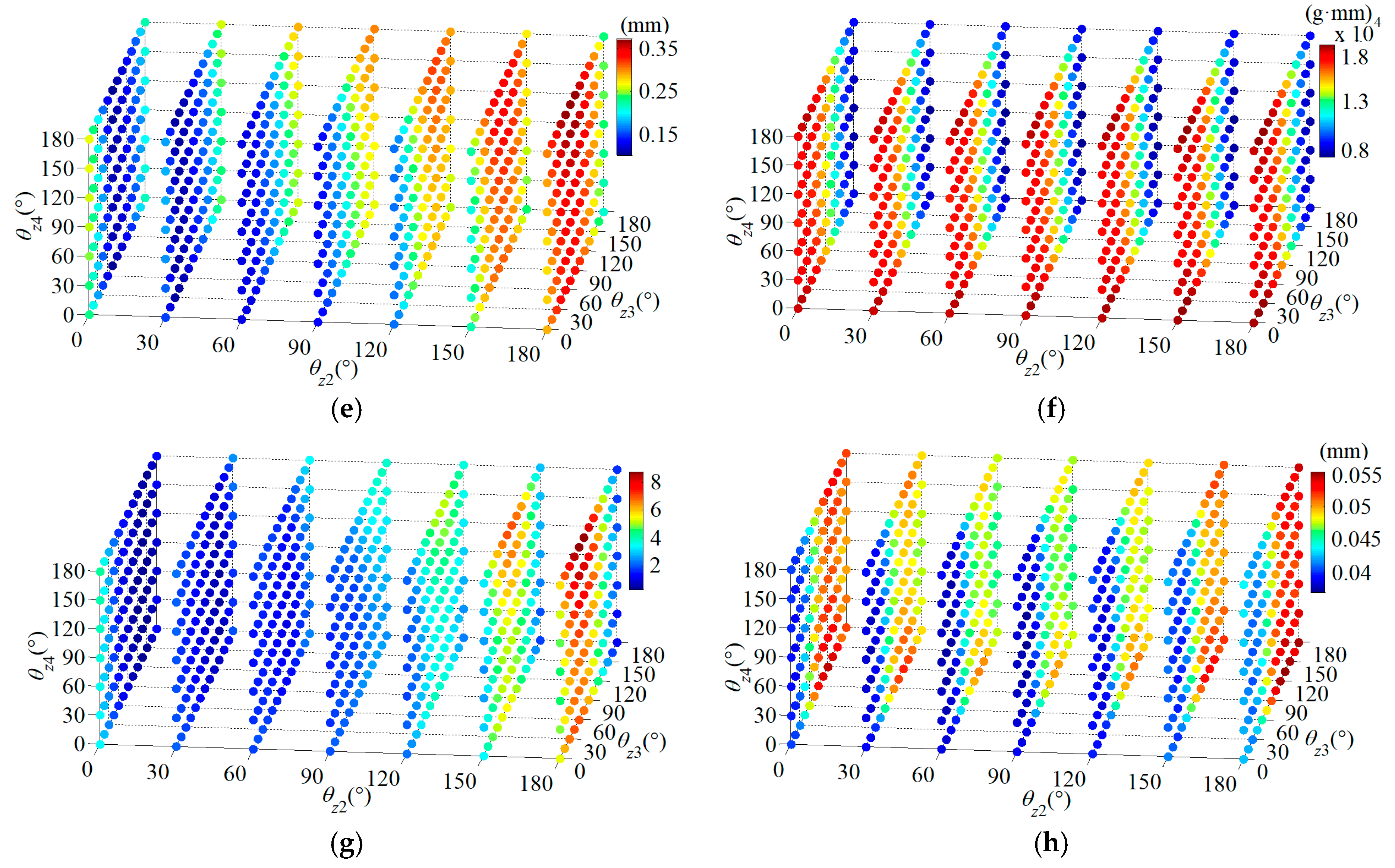
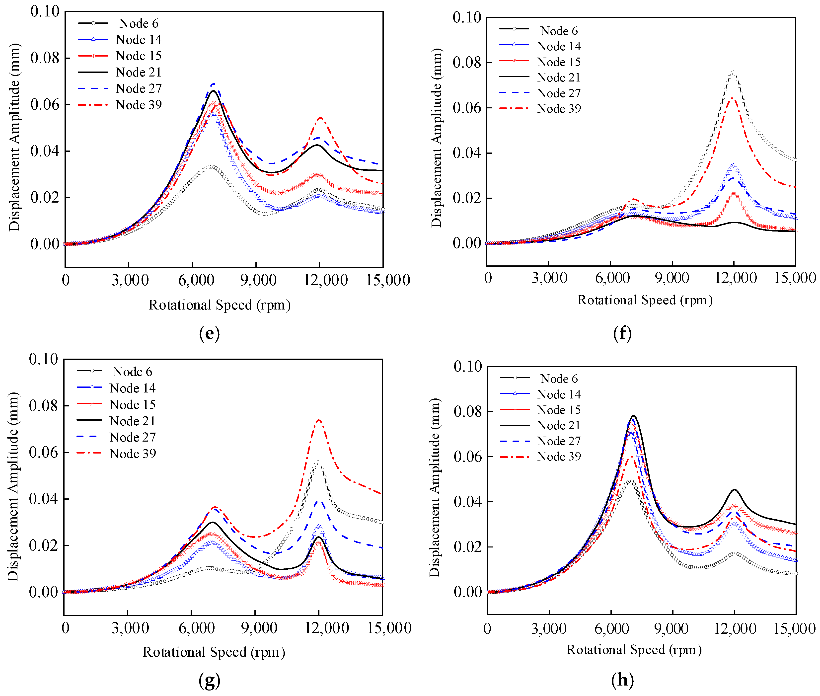
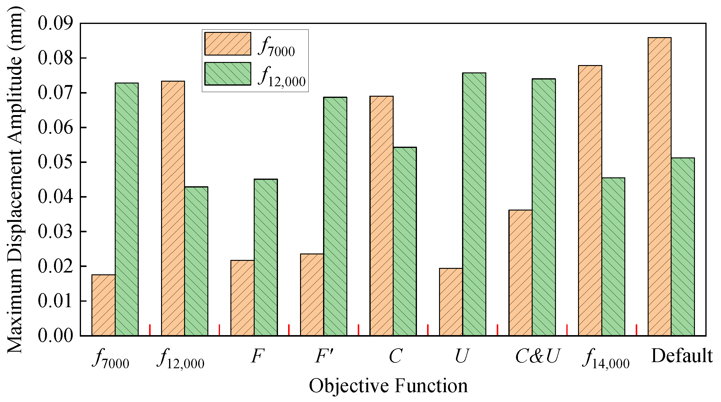
Figure 23 shows the exhaustive search results for these eight objective functions. The four-stage rotor was then assembled and subjected to a run-up test eight separate times, once for each optimal sequence. Figure 24 presents the measured run-up curves of the displacement amplitude across the six nodes under these eight optimal assembly angle sequences.

Table 5. Maximum displacement amplitude across the six nodes under the optimal assembly states obtained using the eight optimization objectives.

Objective Function	Optimal Assembly Angle Sequence	f7000(θz2, θz3, θz4) (mm)	f12,000(θz2, θz3, θz4) (mm)
f7000 (θz2, θz3, θz4)	θz2 = 60°, θz3 = 180°, θz4 = 60°	0.0176	0.0728
f12,000 (θz2, θz3, θz4)	θz2 = 90°, θz3 = 60°, θz4 = 150°	0.0733	0.0429
F(θz2, θz3, θz4)	θz2 = 180°, θz3 = 90°, θz4 = 120°	0.0217	0.0451
F′(θz2, θz3, θz4)	θz2 = 60°, θz3 = 165°, θz4 = 60°	0.0236	0.0687
C(θz2, θz3, θz4)	θz2 = 0°, θz3 = 75°, θz4 = 180°	0.0690	0.0543
U(θz2, θz3, θz4)	θz2 = 90°, θz3 = 180°, θz4 = 90°	0.0194	0.0757
C&U(θz2, θz3, θz4)	θz2 = 0°, θz3 = 135°, θz4 = 60°	0.0362	0.0740

lists the measured maximum displacement amplitudes across the six nodes at the first and second critical speeds under the aforementioned eight optimal sequences. Integrating these results with those from the default assembly angle sequence, a comparative bar chart is plotted (Figure 25).

5. Discussion

First, the effectiveness of the three objective functions constructed in this work—f₇₀₀₀(θ_z2, θ_z3, θ_z4), f_12,000(θ_z2, θ_z3, θ_z4) and F(θ_z2, θ_z3, θ_z4)—in suppressing the vibration response of the four-stage rotor at the first and second critical speeds is examined:

• Compared to the default assembly, the measured vibration response at the first critical speed is reduced by 79.5% when using f₇₀₀₀(θ_z2, θ_z3, θ_z4) as the objective function. However, the response at the second critical speed increases by 42.2%.
• Compared to the default assembly, the measured vibration responses at the first and second critical speeds are reduced by 14.7% and 16.2%, respectively, when using f_12,000(θ_z2, θ_z3, θ_z4) as the objective function.

Compared to the default assembly, the measured vibration responses at the first and second critical speeds are reduced by 74.7% and 11.9%, respectively, when using the normalized objective function F(θ_z2, θ_z3, θ_z4).

Second, the effectiveness of the four objective functions from existing studies—C (θ_z2, θ_z3, θ_z4), U (θ_z2, θ_z3, θ_z4), C&U (θ_z2, θ_z3, θ_z4) and f_14,000(θ_z2, θ_z3, θ_z4)—is examined:

• Compared to the default assembly, the measured vibration response at the first critical speed is reduced by 19.7% when using C (θ_z2, θ_z3, θ_z4) as the objective function, but the response at the second critical speed increases by 6.1%.
• Compared to the default assembly, the measured vibration response at the first critical speed is reduced by 77.4% when using U (θ_z2, θ_z3, θ_z4) as the objective function, but the response at the second critical speed increases by 47.9%.
• Compared to the default assembly, the measured vibration response at the first critical speed is reduced by 57.9% when using C&U (θ_z2, θ_z3, θ_z4) as the objective function, but the response at the second critical speed increases by 44.5%.
• Compared to the default assembly, the measured vibration responses at the first and second critical speeds are reduced by 9.4% and 11.1%, respectively, when using f_14,000(θ_z2, θ_z3, θ_z4) as the objective function.

Additionally, the function F′(θ_z2, θ_z3, θ_z4), calculated using the model without considering flexible dynamic deflection, shows the following effectiveness compared to the default assembly: the vibration response at the first critical speed is reduced by 72.5%, but the response at the second critical speed increases by 34.2%.

In summary, compared to the default assembly angle sequence, the optimal sequence obtained using the normalized six-node vibration response objective function F(θ_z2, θ_z3, θ_z4) proposed in this study reduces the maximum displacement amplitude across the six nodes at the first and second critical speeds by 74.7% and 11.9%, respectively. This vibration suppression effect is significantly superior to that achieved by the four objective functions from existing studies.

Furthermore, only the objective functions F(θ_z2, θ_z3, θ_z4) and f_14,000(θ_z2, θ_z3, θ_z4) result in a simultaneous reduction in vibration response at both the first and second critical speeds for the four-stage rotor. Among these, F(θ_z2, θ_z3, θ_z4) delivers the best overall vibration suppression performance. This conclusion is consistent with the simulation results from Section 3.2, thereby validating the effectiveness of the multi-stage rotor assembly angle optimization model developed in this research.

6. Conclusions

This study presents a novel assembly optimization model that directly suppresses vibration across multiple critical speeds in multi-stage rotors. It transitions the optimization paradigm from minimizing static parameters (geometric or mass errors) or single-speed responses to holistically minimizing the dynamic vibration response during the entire run-up process, with a focus on critical speed traversal. The key contributions are:

• A critical-speed-centric objective function: A new normalized function explicitly minimizes the overall vibration amplitude at the first and second critical speeds across multiple rotor nodes. This addresses the core requirement for safe critical speed passage, which prior studies focusing solely on operational speed vibration overlooked.
• Holistic vibration assessment: The function aggregates data from six key nodes, ensuring suppression of global rotor vibrations rather than isolated bearing vibrations, yielding a more comprehensive performance indicator.
• An integrated assembly optimization model: By coupling an assembly error propagation model with a flexible rotor dynamic model, a complete workflow was established. This model effectively links assembly angle sequences to predictable critical-speed vibrations, enabling efficient optimization via a genetic algorithm.
• Experimental validation and superiority: Tests on a four-stage rotor confirmed the model’s effectiveness. The optimal sequence achieved balanced vibration reductions of 74.7% and 11.9% at the first and second critical speeds, significantly outperforming conventional methods based on geometric concentricity, mass unbalance, or single-speed vibration.

In summary, this work provides a direct, vibration-suppression-oriented strategy for multi-stage rotor assembly. Moving beyond traditional error compensation, it offers a practical methodology to enhance operational safety and reliability by ensuring low-vibration traversal through critical speeds.

References

1. Chen, Y.; Cui, J.; Sun, X. An Unbalance Optimization Method for a Multi-Stage Rotor Based on an Assembly Error Propagation Model. Appl. Sci. 2021, 11, 887. [Google Scholar] [CrossRef]
2. Chen, Y.; Cui, J.; Sun, X. Research on Multistage Rotor Assembly Optimization Methods for Aeroengine Based on the Genetic Algorithm. Complexity 2021, 2021, 8847690. [Google Scholar] [CrossRef]
3. Hussain, T.; Yang, Z.; Popov, A.A.; McWilliam, S. Straight-build assembly optimization: A method to minimize stage-by-stage eccentricity error in the assembly of axisymmetric rigid components (two-dimensional case study). J. Manuf. Sci. Eng. 2011, 133, 141–149. [Google Scholar] [CrossRef]
4. Hussain, T.; McWilliam, S.; Popov, A.A.; Yang, Z. Geometric error reduction in the assembly of axis-symmetric rigid components: A two-dimensional case study. Proc. Inst. Mech. Eng. Part B J. Eng. Manuf. 2012, 226, 1259–1274. [Google Scholar] [CrossRef]
5. Hussain, T.; Yasinshaikh, G.; Shaikh, S.A. Variation propagation control in straight-build assemblies: 2D case study. Mehran Univ. Res. J. Eng. Technol. 2013, 32, 71–80. [Google Scholar]
6. Yang, Z.; Popov, A.A.; McWilliam, S. Variation propagation control in mechanical assembly of cylindrical components. J. Manuf. Syst. 2012, 31, 162–176. [Google Scholar] [CrossRef]
7. Yang, Z.; Hussain, T.; Popov, A.A.; McWilliam, S. A comparison of different optimization techniques for variation propagation control in mechanical assembly. In Proceedings of the International Conference on Materials Science and Engineering, Sheffield, UK, 9–10 September 2011; IOP Publishing: Bristol, UK, 2011; Volume 26. [Google Scholar]
8. Yang, Z.; Hussain, T.; Popov, A.A.; McWilliam, S. Novel optimization technique for variation propagation control in an aero-engine assembly. Proc. Inst. Mech. Eng. Part B J. Eng. Manuf. 2011, 225, 100–111. [Google Scholar] [CrossRef]
9. Yang, Z.; McWilliam, S.; Popov, A.A.; Hussain, T.; Yang, H. Dimensional variation propagation analysis in straight-build mechanical assemblies using a probabilistic approach. J. Manuf. Syst. 2013, 32, 348–356. [Google Scholar] [CrossRef]
10. Wang, L.; Sun, C.; Tan, J.; Zhao, B.; Wan, G. Improvement of location and orientation tolerances propagation control in cylindrical components assembly using stack-build assembly technique. Assem. Autom. 2015, 35, 358–366. [Google Scholar] [CrossRef]
11. Sun, C.; Li, C.; Liu, Y.; Liu, Z.; Wang, X.; Tan, J. Prediction method of concentricity and perpendicularity of aero engine multistage rotors based on PSO-BP neural network. IEEE Access 2019, 7, 132271–132278. [Google Scholar] [CrossRef]
12. Sun, C.; Liu, Z.; Liu, Y.; Wang, X.; Tan, J. An adjustment method of geometry and mass centers for precision rotors assembly. IEEE Access 2019, 7, 169992–170002. [Google Scholar] [CrossRef]
13. Sun, Y.; Guo, J.; Hong, J.; Liu, G.; Wu, W.; Yue, C. Repair decision based on sensitivity analysis for aero engine assembly. Int. J. Precis. Eng. Manuf. 2019, 20, 347–362. [Google Scholar] [CrossRef]
14. Ding, S.; Jin, S.; Li, Z.; Wei, Z.; Zang, F. Deviation Propagation Model and Optimization for Aero-Engine Rotor Assembly Concentricity. J. Shanghai Jiao Tong Univ. 2018, 52, 9. [Google Scholar]
15. Sun, J.; Ding, S.; Li, Z.; Yang, F.; Ma, X. Point-based solution using Jacobian-Torsor theory into partial parallel chains for revolving components assembly. J. Manuf. Syst. 2018, 46, 46–58. [Google Scholar]
16. Ding, S.; He, Y.; Zheng, X. A probabilistic approach for three-dimensional variation analysis in aero-engine rotors assembly. Int. J. Aeronaut. Space Sci. 2021, 22, 1092–1105. [Google Scholar] [CrossRef]
17. Tu, J.; Li, Z.; Ge, H.; Liu, L.; Liu, H.H. Multi-objective Optimization of Rotor Stack Assembly Based on Geometric Algebra Theory. Acta Aeronaut. Astronaut. Sin. 2021, 42, 524197. [Google Scholar]
18. Liu, Y.; Zhang, M.; Sun, C.; Hu, M.; Chen, D.; Liu, Z.; Tan, J. A method to minimize stage-by-stage initial unbalance in the aero engine assembly of multistage rotors. Aerosp. Sci. Technol. 2019, 85, 270–276. [Google Scholar] [CrossRef]
19. Chen, Y.; Cui, J.; Sun, X. An assembly method for the multistage rotor of an aero-engine based on the dual objective synchronous optimization for the coaxality and unbalance. Aerospace 2021, 8, 94. [Google Scholar] [CrossRef]
20. Sun, C.; Li, R.; Chen, Z.; Mei, Y.; Wang, X.; Li, C.; Liu, Y. Research on vibration suppression method based on coaxial stacking measurement. Mathematics 2021, 9, 1438. [Google Scholar] [CrossRef]
21. Liu, Y.; Li, R.; Sun, C.; Chen, Z.; Mei, Y.; Xiao, P.; Wang, X.; Li, C. Research on rotary parts vibration suppression based on coaxiality measurement and unbalance constraint. Appl. Sci. 2021, 11, 5747. [Google Scholar] [CrossRef]
22. Liu, Y.; Mei, Y.; Sun, C.; Xiao, P.; Li, R.; Wang, X.; Li, C. Multistage asymmetric rotors coaxial measurement stacking method based on minimization of exciting force. Symmetry 2021, 13, 1054. [Google Scholar] [CrossRef]
23. Chen, Y.; Cui, J.; Sun, X. A vibration suppression method for the multistage rotor of an aero-engine based on assembly optimization. Machines 2021, 9, 189. [Google Scholar] [CrossRef]
24. Bladh, R.; Castanier, M.; Pierre, C. Effects of multistage coupling and disc flexibility on mistuned bladed disk dynamics. J. Eng. Gas Turbines Power 2003, 125, 121–130. [Google Scholar] [CrossRef]
25. Shahab, A.A.S.; Thomas, J. Coupling effects of disc flexibility on the dynamics behavior of multi disc-shaft system. J. Sound Vib. 1987, 114, 435–452. [Google Scholar] [CrossRef]
26. Laxalde, D.; Lombard, J.-P.; Thouverez, F. Dynamics of multi-stage bladed disks systems. In Proceedings of the ASME Turbo Expo 2007: Power for Land, Sea and Air, Montreal, QC, Canada, 1–14 May 2007. [Google Scholar]
27. Rzadkowski, R.; Maurin, A. Multistage Coupling of Eight Mistuned Bladed Disks on a Solid Shaft of the Steam Turbine, Forced Vibration Analysis. J. Vib. Eng. Technol. 2014, 2, 495–508. [Google Scholar]
28. Goldberg, D.E. Genetic Algorithms in Search, Optimization, and Machine Learning; Addison-Wesley: Boston, MA, USA, 1989. [Google Scholar]
29. Chen, Y.; Liu, G.Y.; Jia, Y.H. A Vibration Response Prediction Model for Multi-Stage Assembled Rotors Based on Synchronous Excitation of Mass Eccentricity Error and Spigot Eccentricity Error. Aerospace 2026, 13, 218. [Google Scholar] [CrossRef]
Figure 1. Model for searching optimal assembly angles to minimize multi-stage rotor vibration.
Aerospace 13 00310 g001
Figure 2. Measurement definition of the assembly spigot for a single-stage rotor.
Aerospace 13 00310 g002
Figure 3. Geometric parameters of a single-stage rotor.
Aerospace 13 00310 g003
Figure 4. Mass parameters of a single-stage rotor.
Aerospace 13 00310 g004
Figure 5. A two-stage rotor assembly.
Aerospace 13 00310 g005
Figure 6. Decomposition of two-plane unbalance in a rotor dynamic balance test.
Aerospace 13 00310 g006
Figure 7. Decomposition of the two-plane unbalance of a two-stage rotor.
Aerospace 13 00310 g007
Figure 8. Finite element model of the four-stage assembled rotor.
Aerospace 13 00310 g008
Figure 9. Campbell diagram of the four-stage assembled rotor.
Aerospace 13 00310 g009
Figure 10. Validation results from the refined commercial FEM model.
Aerospace 13 00310 g010
Figure 11. Maximum displacement amplitude across the six nodes with f7421(θz2, θz3, θz4) as the objective function: (a) Convergence curve of the genetic optimization for f7421(θz2, θz3, θz4); (b) Exhaustive search results of f7421(θz2, θz3, θz4) over all assembly angle sequences.
Aerospace 13 00310 g011
Figure 12. Maximum displacement amplitude across the six nodes with f7421(θz2, θz3, θz4) as the objective function: (a) Optimal assembly angle sequence; (b) Worst assembly angle sequence.
Aerospace 13 00310 g012
Figure 13. Maximum displacement amplitude across the six nodes with f11,810(θz2, θz3, θz4) as the objective function: (a) Convergence curve of the genetic optimization for f11,810(θz2, θz3, θz4); (b) Exhaustive search results of f11,810(θz2, θz3, θz4) over all assembly angle sequences.
Aerospace 13 00310 g013
Figure 14. Maximum displacement amplitude across the six nodes with f11,810(θz2, θz3, θz4) as the objective function: (a) Optimal assembly angle sequence; (b) Worst assembly angle sequence.
Aerospace 13 00310 g014
Figure 15. Maximum displacement amplitude across the six nodes with F(θz2, θz3, θz4) as the objective function: (a) Convergence curve of the genetic optimization for F(θz2, θz3, θz4); (b) Exhaustive search results of F(θz2, θz3, θz4) over all assembly angle sequences.
Aerospace 13 00310 g015
Figure 16. Maximum displacement amplitude across the six nodes with F(θz2, θz3, θz4) as the objective function: (a) Optimal assembly angle sequence; (b) Worst assembly angle sequence.
Aerospace 13 00310 g016
Figure 17. Convergence curves of multiple independent runs using f 7421 ( θ z 2 , θ z 3 , θ z 4 ) as the objective function: (a) Second independent run; (b) Third independent run.
Aerospace 13 00310 g017
Figure 18. Maximum displacement amplitude across the six nodes under the default assembly angle sequence.
Aerospace 13 00310 g018
Figure 19. Exhaustive search results of the four objective functions over all assembly angle sequences: (a) Exhaustive search results for C (θz2, θz3, θz4); (b) Exhaustive search results for U (θz2, θz3, θz4); (c) Exhaustive search results for C&U (θz2, θz3, θz4); (d) Exhaustive search results for f17,000(θz2, θz3, θz4).
Aerospace 13 00310 g019
Figure 20. Maximum displacement amplitude across the six nodes at the first and second critical speeds (7421 rpm and 11,810 rpm) under the optimal assembly angle sequences obtained by different objective functions.
Aerospace 13 00310 g020
Figure 21. Vibration test setup for the four-stage rotor.
Aerospace 13 00310 g021
Figure 22. Run-up curves of the displacement amplitude across six nodes from 0 to 15,000 rpm.
Aerospace 13 00310 g022
Figure 23. Exhaustive search results of the eight objective functions over all assembly angle sequences: (a) Exhaustive search results for f7000z2, θz3, θz4); (b) Exhaustive search results for f12,000z2, θz3, θz4); (c) Exhaustive search results for F(θz2, θz3, θz4); (d) Exhaustive search results for F′(θz2, θz3, θz4); (e) Exhaustive search results for C (θz2, θz3, θz4); (f) Exhaustive search results for U (θz2, θz3, θz4); (g) Exhaustive search results for C&U (θz2, θz3, θz4); (h) Exhaustive search results for f14,000(θz2, θz3, θz4).
Aerospace 13 00310 g023aAerospace 13 00310 g023b
Figure 24. Run-up curves of the displacement amplitude across the six nodes under the optimal assembly angle sequences obtained from the eight objective functions: (a) f7000z2, θz3, θz4); (b) f12,000z2, θz3, θz4); (c) F(θz2, θz3, θz4); (d) F′(θz2, θz3, θz4); (e) C (θz2, θz3, θz4); (f) U (θz2, θz3, θz4); (g) C&U (θz2, θz3, θz4); (h) f14,000(θz2, θz3, θz4).
Aerospace 13 00310 g024aAerospace 13 00310 g024b
Figure 25. Maximum displacement amplitude across the six nodes at the first and second critical speeds (7000 rpm and 12,000 rpm) under the optimal assembly angle sequences obtained by different objective functions.
Aerospace 13 00310 g025