Multi-Objective Optimization of an Adaptive Cycle Fan Based on XAI-Driven Feature Selection

Abstract

To address the high-dimensional design optimization of an adaptive cycle fan (ACF), this paper proposes a new multi-objective optimization (MOO) method based on explainable artificial intelligence (XAI)-driven feature selection. The proposed method integrates a neural network surrogate model, Shapley additive explanation (SHAP) analysis, and a genetic algorithm. By considering Pareto front quality, surrogate model accuracy, and optimization preference, a composite evaluation metric, Q, is defined to guide a bidirectional feature selection process based on SHAP analysis, thereby establishing a dynamic, closed-loop process of simultaneous feature selection and MOO. The results indicate that the proposed method significantly enhances global search capability, accurately identifying 66 optimal features from 119 initial features. A further comparison with results without forward selection confirms the necessity of dynamically adjusting the feature space during optimization. Under the same condition, the optimal design increases the core pressure ratio from 2.71 to 2.81 and core efficiency from 80.80% to 82.92%. The flow mechanism analysis reveals that the performance gains mainly result from the reconstruction of shock structures and the suppression of shock–boundary layer interactions and secondary flows. The XAI-enhanced surrogate-assisted evolutionary algorithm (SAEA) proposed in this paper provides a promising methodology for high-dimensional MOO of aeroengines and other complex systems.

1. Introduction

The adaptive cycle engine (ACE) adjusts variable geometry components to change cycle parameters such as mass flow, bypass ratio, and pressure ratio, thereby changing the engine’s operating condition and maintaining optimal performance over the full flight envelope. It can satisfy both the fuel consumption requirement in subsonic flight and the thrust requirement in supersonic flight, and is therefore regarded as a core technology for next-generation aero-propulsion systems [1,2]. The ACF is a key component of the ACE and plays a critical role in realizing variable cycle characteristics.

An ACF typically consists of multistage fans and features multi-bypass configurations, making it a typical high-dimensional nonlinear optimization problem. However, in such a high-dimensional design space, as the number of design variables increases, the volume of the sample space expands exponentially, leading to a dramatic increase in the cost of high-fidelity computations or physical experiments, and thus triggering the “curse of dimensionality.”

Facing the high costs of computational fluid dynamics (CFD) simulations and physical experiments, SAEAs have gradually superseded traditional exhaustive search methods as the mainstream method for turbomachinery aerodynamic optimization [3]. Early studies mainly focused on low-dimensional problems and verified the effectiveness of the method. Benini et al. [4,5] performed Pareto optimization of NASA Rotor 37 using multi-objective evolutionary algorithms and successfully improved the pressure ratio and efficiency of the transonic rotor. Lian et al. [6] combined a response surface model to achieve lightweight and high-performance design of NASA Rotor 67. With further research, to address more complex problems, Xiong et al. [7] developed a multi-model ensemble optimization strategy for large-scale fans, improving global search robustness by dynamically weighting different surrogate models. Zhao et al. [8] proposed an efficient framework based on a “pre-screening” mechanism, using a low-fidelity model to rapidly eliminate inferior solutions and significantly improving optimization efficiency for high-loaded compressors in heavy-duty gas turbines. Long et al. [9] proposed a surrogate-assisted differential evolution algorithm based on a manifold learning sampling strategy, which guides efficient sampling by capturing low-dimensional manifold structures in high-dimensional objective spaces to solve high-dimensional optimization challenges under complex aerodynamic constraints.

Although SAEAs perform well for low-dimensional optimization, they still face a severe “curse of dimensionality” in the high-dimensional design spaces brought by the refined design of modern high-performance turbomachinery. He et al. [10] pointed out that high-dimensional design spaces not only dilute sample point distributions, leading to a sharp drop in surrogate model accuracy, but also significantly slow down the convergence of evolutionary algorithms. Jin [11] summarized that effectively managing surrogate models and extracting key information from high-dimensional spaces is one of the core challenges for future SAEAs under limited computational resources. To alleviate modeling pressure in high-dimensional spaces, dimension reduction and feature selection techniques have become research hotspots. Hou et al. [12] systematically reviewed dimension-reduction methods in engineering design and concluded that feature selection can significantly reduce modeling complexity while improving surrogate accuracy. In specific applications, Bird et al. [13] compared principal component analysis and nonlinear manifold learning for compressor blade optimization and verified the potential of dimension reduction for real-time performance prediction. For manufacturing and operational uncertainties, Wang et al. [14] proposed a feature-selection-based high-dimensional uncertainty quantification method, identifying 41 features affecting mass flow and 66 features affecting efficiency from 291 uncertainty features; on this basis, Wang et al. [15] further used this method to accurately identify the 15 most critical features responsible for performance dispersion in a multistage compressor, enabling low-cost robustness control.

With the development of artificial intelligence, surrogate models in SAEAs have evolved from early response surface models, Kriging models, or radial basis function models toward higher-order machine learning models such as neural networks and deep learning [16]. Owing to strong nonlinear approximation capability, these models show greater predictive potential in high-dimensional spaces; however, their inherent “black box” nature introduces new challenges. In recent years, advances in XAI have provided new methods for “black box” optimization, and improving the transparency and decision reliability of optimization algorithms using XAI is an important future direction [17]. XAI techniques represented by SHAP [18] provide interpretability for surrogate models. In optimization, Li et al. [19] introduced XAI into an SAEA framework and used interpretable machine learning models to analyze population features, guiding crossover and mutation operations and significantly accelerating convergence for MOO. For design space exploration, Palar et al. [20] proposed a multi-objective exploration method based on interpretable surrogate models and used SHAP to analyze complex relationships among wing design variables. For turbomachinery, Wang et al. [21] used SHAP to analyze the influence of geometric uncertainty on a transonic rotor’s performance deviation and the underlying mechanisms under different operating conditions. Cheng et al. [22] developed a fan aerodynamic robustness optimization platform based on interpretable dynamic machine learning, demonstrating the advantages of XAI in improving design reliability.

At present, SAEAs still play a key role in addressing the MOO problems of high-dimensional complex systems. However, a review of past studies reveals certain limitations. In dimension reduction or feature selection, most studies adopt a “static” strategy, i.e., selecting features based on initial samples before optimization and removing features deemed unimportant to reduce dimensionality. This static treatment has significant limitations because it ignores the dynamic evolution of feature importance during optimization. Some recent studies have begun to introduce adaptive spaces to alleviate the curse of dimensionality, which also reflects the necessity of dynamically adjusting the feature space during iterations [23]. Some features may appear to have little impact on objectives at the early stage but may play a key role for small performance variations in local regions near the Pareto front. If such features are permanently eliminated in the early stages, the optimizer may fail to converge to the real global optimum at later stages. In addition, although XAI has shown great potential in aerodynamic optimization design, most existing studies treat it as a “post hoc analysis” tool rather than transforming its interpretability into an active optimization strategy.

Therefore, this paper proposes a new MOO method based on XAI-driven feature selection. The method integrates neural network surrogate model, SHAP analysis, and genetic algorithm. By comprehensively considering Pareto-front quality, surrogate model accuracy, and optimization preference, a composite evaluation indicator, Q, is defined as a feedback signal. This indicator guides a bidirectional feature selection process based on SHAP analysis, thereby establishing a dynamic, closed-loop process of simultaneous feature selection and MOO. Using this method, benchmark test data are first generated with mathematical functions to validate accuracy. The method is then applied to high-dimensional aerodynamic optimization of an ACF, obtaining a globally optimal Pareto front, selecting the optimal features, and analyzing the composition and sensitivity of features. Next, by comparing with a static feature selection strategy (i.e., without forward selection), the necessity of dynamically adjusting the feature space during optimization is further confirmed. Finally, the optimal design is determined based on the MOO results, and by analyzing the flow mechanisms underlying performance gains, the consistency between flow field improvements and feature selection results is verified.

2. Case Description

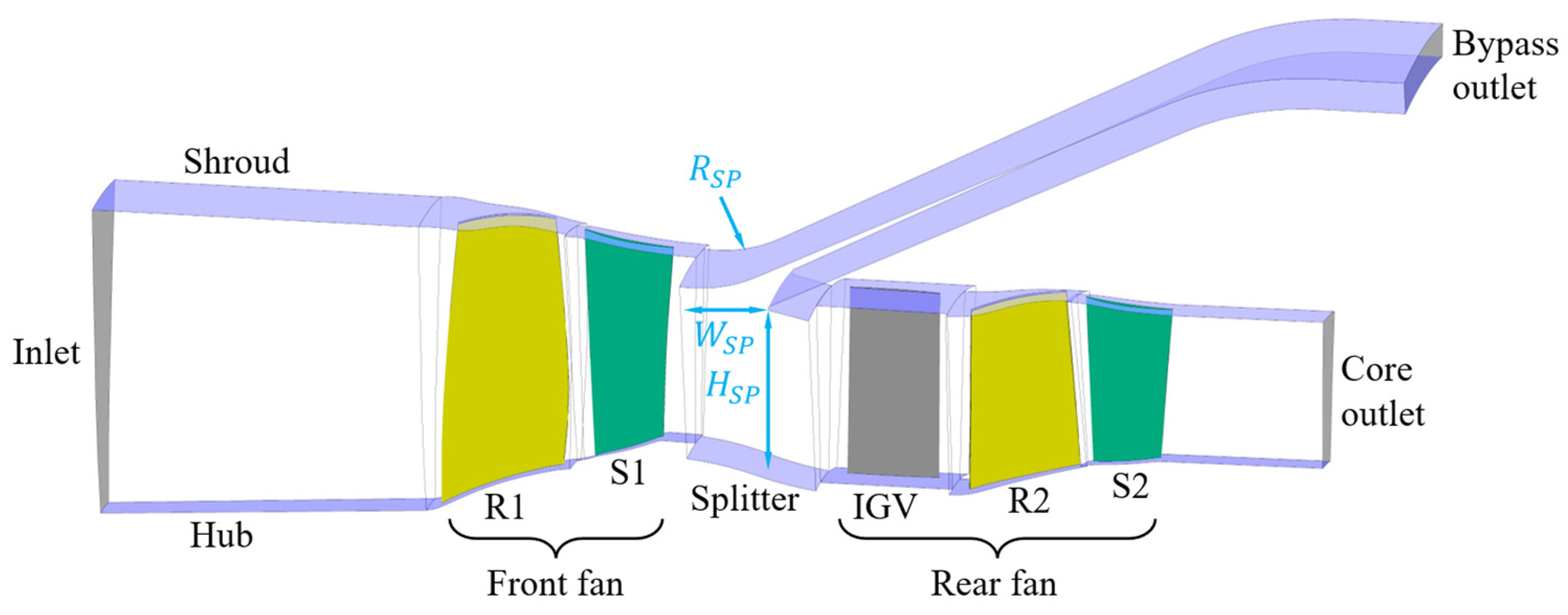
According to the overall design requirements of an ACE, the ACF investigated in this paper adopts a dual-bypass configuration, as shown in Figure 1. It features a separated-stage architecture, comprising a single-stage front fan and a single-stage rear fan. The front fan operates without an inlet guide vane (IGV) and consists of one row of rotor blades and one row of stator vanes; in contrast, the rear fan consists of one row of IGVs, one row of rotor blades and one row of stator vanes. By adjusting the back pressure or mass flow at the core and bypass outlets, the operating condition of the ACF can be changed. Some of the key design parameters of the investigated ACF are listed in

Table 1. Key design parameters of the ACF.

Parameter	Value
Front fan pressure ratio (S1 outlet to ACF inlet)	1.8
Rear fan pressure ratio (core outlet to IGV inlet)	1.5
Bypass ratio (bypass mass flow to core mass flow)	0.10
Flow coefficient (ratio of axial velocity to R1 mid-span speed)	0.41
R1 tip Mach number (relative inlet Mach number at R1 tip)	1.63
R1 hub-to-tip radius ratio (hub radius to tip radius at R1 inlet)	0.39
R1 tip solidity (ratio of blade chord length to circumferential pitch at R1 tip)	1.59

, indicating that it represents a typical highly loaded ACF with a low bypass ratio.

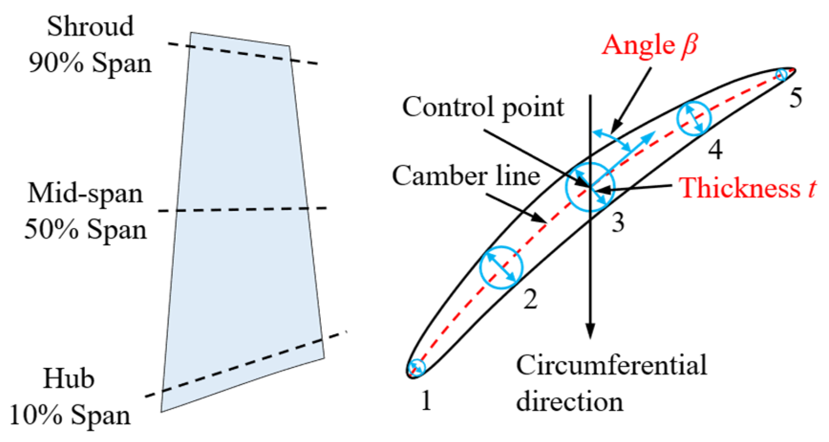
For design optimization, parameterization is first required to extract the design features of blades and flow paths. The blade parameterization is shown in Figure 2. Specific spanwise sections are selected: 10% (hub), 50% (mid-span), and 90% (shroud) spans for rotor blades; and 10% and 90% spans for the IGV and stator vanes. Control points are distributed along the camber line of each section from the leading edge to the trailing edge. Specifically, five control points are assigned to rotor blades and stator vanes, while three are used for the IGV. At each control point, an angle parameter ($\beta$) and a thickness parameter ($t$) are defined. To clarify the nomenclature, taking ${\beta }_{R1M3}$ as an example, the subscript ’R1’ denotes the specific component (front fan rotor), ‘M’ indicates the spanwise location (Mid-span, i.e., 50% span, alongside ‘H’ for Hub and ‘S’ for Shroud), and ‘3’ refers to the sequential number of the geometric control point along the camber line (the third out of five points). Thus, this parameter represents the angle at the third control point on the 50% span section of the front fan rotor; other parameters are defined analogously. In addition, the tip clearances of the front fan rotor (${\delta }_1$) and rear fan rotor (${\delta }_2$) are considered. For the splitter, three parameters are defined: transition radius ($R_{SP}$), axial width ($W_{SP}$), and radial height ($H_{SP}$), as shown in Figure 1. Moreover, since the variations in features alter the ACF performance and operating point, two operating condition parameters are included, namely the core outlet back pressure (PbC) and the bypass outlet back pressure (PbB), to analyze the influence of operating condition variations. In total, 119 features are defined, with detailed definitions provided in

Table 2. Definition of the initial 119 design parameters of the ACF.

Location	Parameter	Number
R1	${\beta }_{R1H1}$–${\beta }_{R1H5}$, ${\beta }_{R1M1}$–${\beta }_{R1M5}$, ${\beta }_{R1S1}$–${\beta }_{R1S5}$, $t_{R1H1}$–$t_{R1H5}$, $t_{R1M1}$–$t_{R1M5}$, $t_{R1S1}$–$t_{R1S5}$, ${\delta }_1$	31
S1	${\beta }_{S1H1}$–${\beta }_{S1H5}$, ${\beta }_{S1S1}$–${\beta }_{S1S5}$ $t_{S1H1}$–$t_{S1H5}$, $t_{S1S1}$–$t_{S1S5}$	20
Splitter	$R_{SP}$, $W_{SP}$, $H_{SP}$	3
IGV	${\beta }_{IGH1}$–${\beta }_{IGH3}$, ${\beta }_{IGS1}$–${\beta }_{IGS3}$ $t_{IGH1}$–$t_{IGH3}$, $t_{IGS1}$–$t_{IGS3}$	12
R2	${\beta }_{R2H1}$–${\beta }_{R2H5}$, ${\beta }_{R2M1}$–${\beta }_{R2M5}$, ${\beta }_{R2S1}$–${\beta }_{R2S5}$, $t_{R2H1}$–$t_{R2H5}$, $t_{R2M1}$–$t_{R2M5}$, $t_{R2S1}$–$t_{R2S5}$, ${\delta }_2$	31
S2	${\beta }_{S2H1}$–${\beta }_{S2H5}$, ${\beta }_{S2S1}$–${\beta }_{S2S5}$ $t_{S2H1}$–$t_{S2H5}$, $t_{S2S1}$–$t_{S2S5}$	20
Outlet	PbC, PbB	2
Total number of features		119

. The total number of parameters in the last column of Table 2 is systematically calculated. For instance, the 31 variables for the front fan rotor consist of 30 profile parameters (3 spanwise sections $\times$ 5 control points per section $\times$ 2 parameter types, namely $\beta$ and $t$) plus 1 tip clearance parameter (${\delta }_1$). Other numbers are calculated similarly.

In this paper, six key performance parameters of the ACF are evaluated: total mass flow ${\dot{m}}_{tot}$, bypass ratio $bpr$, core pressure ratio ${\pi }_C$, core efficiency ${\eta }_C$, bypass pressure ratio ${\pi }_B$, and bypass efficiency ${\eta }_B$. Since the core mass flow ${\dot{m}}_C$ and bypass mass flow ${\dot{m}}_B$ can be derived from these variables, these six parameters are selected as the study outputs. The core and bypass pressure ratios are defined as the ratios of the total pressure at their respective outlets to the inlet total pressure. Correspondingly, the core and bypass efficiencies are calculated based on the associated pressure and temperature ratios.

3. Methodology

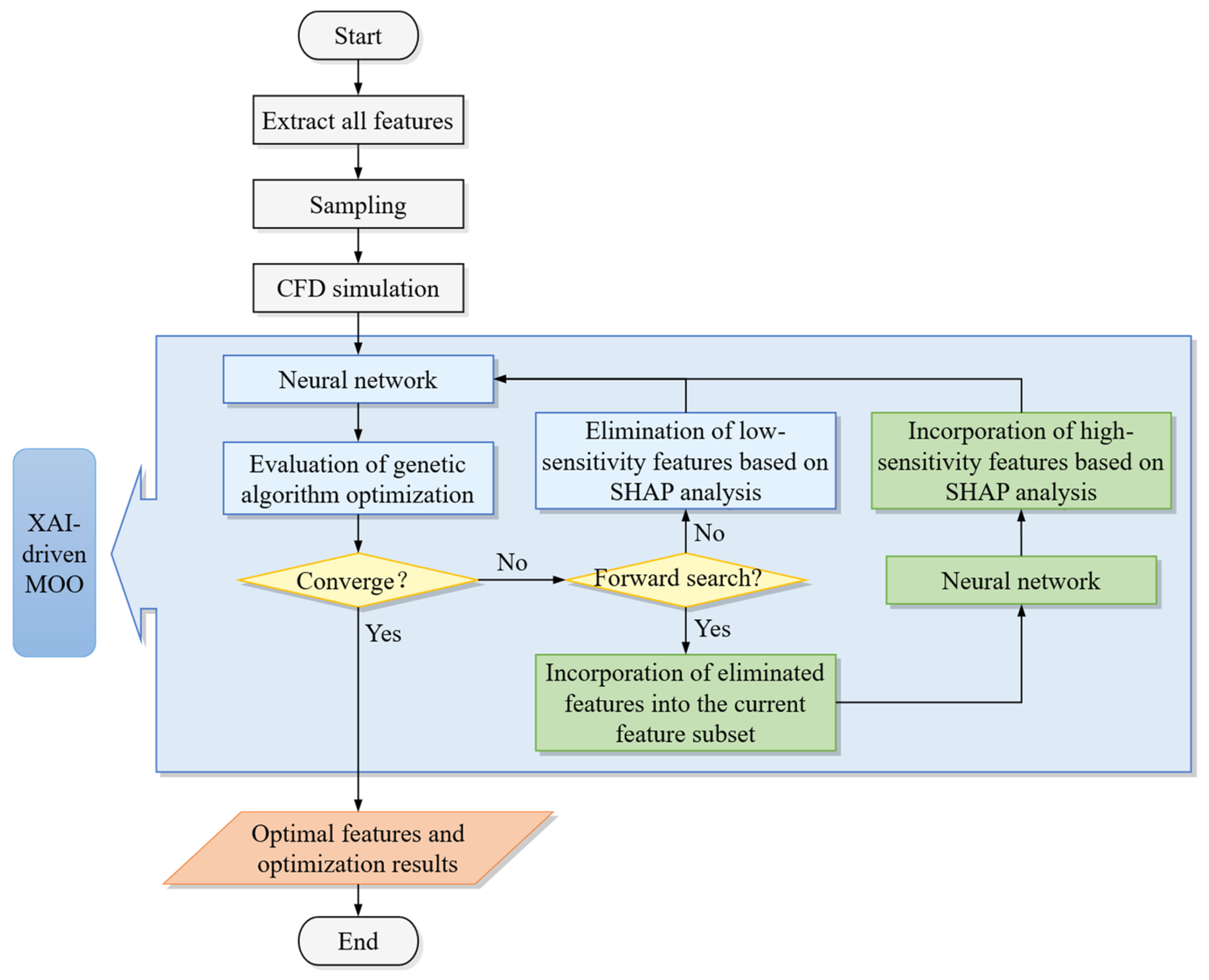
This paper proposes a new MOO method based on XAI-driven feature selection, as illustrated in Figure 3. First, parameterization is performed to extract all design features. Due to the large number of features and the high dimensionality of the problem, sampling is employed to construct the sample space. Then, CFD simulations are conducted to evaluate the ACF performance at the sampled points. A neural network is then utilized to establish a surrogate model that maps input features to performance parameters. This surrogate model serves as the evaluation function, and a genetic algorithm is executed for optimization within the search space defined by the current feature subset. Based on the optimization results, the feature selection strategy is determined. SHAP is used to compute feature importance; low-sensitivity features are eliminated via backward selection, while high-sensitivity features are incorporated via forward selection. Consequently, the feature subset is dynamically updated and iterated during the optimization process, ensuring that the MOO converges to the global optimum. The proposed method establishes a dynamic closed-loop iteration of feature selection and MOO. This approach overcomes the limitations of static feature selection and effectively prevents the optimization process from becoming trapped in local optima, thereby yielding global optimal solutions. Furthermore, by leveraging SHAP as the core XAI tool, its interpretability is utilized not only for post hoc analysis but also to directly inform updates to the feature space, further improving the method’s accuracy. Detailed descriptions are provided below.

3.1. Sampling Method

To improve sampling efficiency while ensuring computational accuracy and to fully explore the design space of high-dimensional variables, Latin hypercube sampling (LHS) is adopted for the design of experiments. LHS, first proposed by McKay et al. [24] in 1979, is a multi-dimensional stratified sampling technique capable of efficiently generating a representative sample set from multivariate parameter distributions. In contrast to traditional simple random sampling (e.g., Monte Carlo sampling), LHS demonstrates superior space-filling properties and significant variance reduction [25]. For a given sample size, LHS avoids sample clustering and ensures that sample points are uniformly distributed throughout the hypercube space, covering the full ranges of all variables while capturing nonlinear relationships. Therefore, more accurate statistical estimates can be obtained at a lower computational cost. In this paper, LHS is used to generate the sample space of input features, providing a reliable dataset for subsequent studies.

3.2. Numerical Method

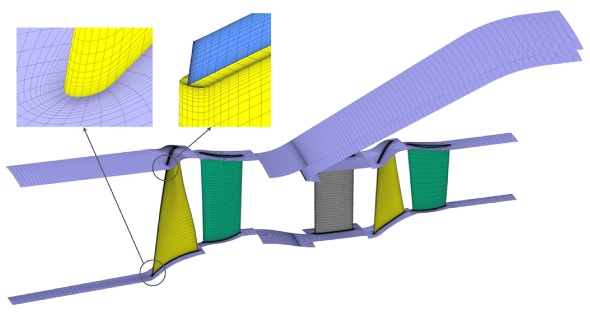
In this paper, three-dimensional CFD simulations are performed using ANSYS CFX 19.2, a commercial turbomachinery simulation software. Single-passage structured meshes are generated using TurboGrid and ICEM, as shown in Figure 4. An H-O-H mesh topology is adopted: H-type meshes are used upstream, downstream, and within the passage, while an O-type mesh is applied around the blade to improve mesh quality on blade surfaces. To capture flow details within the rotor tip clearance more accurately, local refinement is performed in the tip-clearance region using an H-type mesh. The face angles of the mesh range from 28° to 161°, meeting the TurboGrid recommendation of 15–165°; the volume ratio is between 1 and 13, which also meets the requirement of being less than 15. The coupled solver, which solves the hydrodynamic equations as a single system with a multigrid-accelerated ILU linear solver, is used [26]. The widely used two-equation SST turbulence model [27] is adopted, as it can accurately capture flow fields with strong adverse pressure gradients and significant boundary-layer separation. The first layer height is set to 0.01 mm to ensure y+ < 1.0, meeting the requirement of the turbulence model. A grid independence study was conducted in our previous work [28], where four different grid densities (1.2 M, 2.1 M, 3.2 M, and 4.6 M) were tested. The grid with 3.2 M elements was selected as an optimal trade-off between computational time and simulation accuracy.

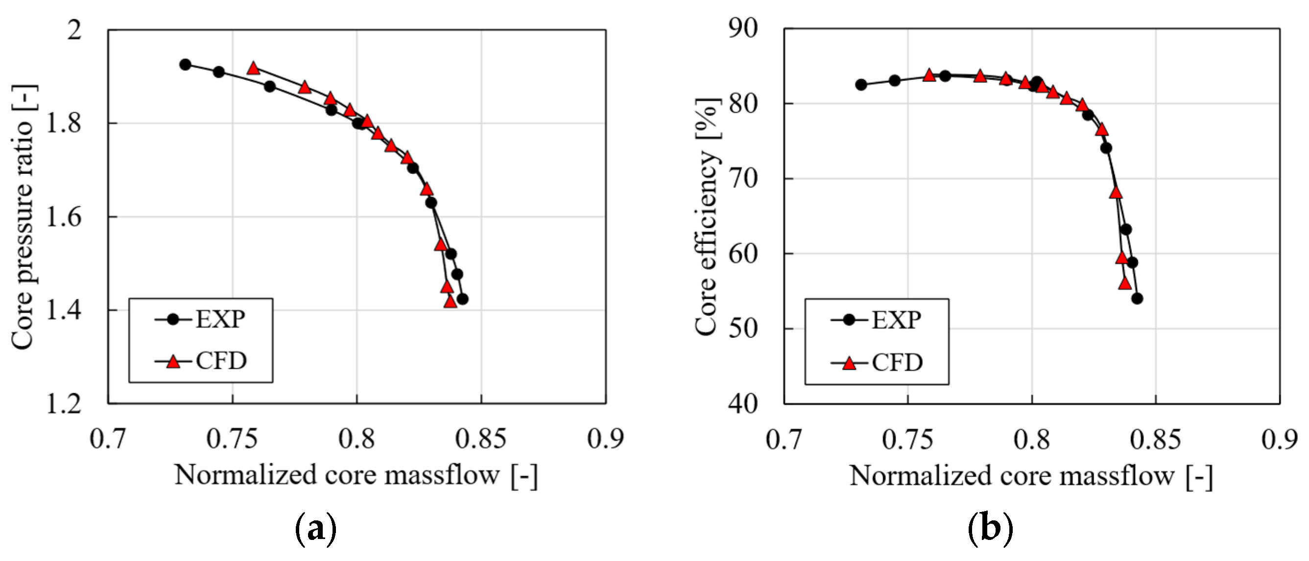
At the inlet, a total temperature of 288.15 K and a total pressure of 101,325 Pa are imposed with axial inflow. Static pressure is specified at the outlets of both the core and bypass. The convergence criterion is defined as residuals falling below 1 × 10⁻⁶ with monitored parameters varying by less than 1%. Furthermore, Figure 5 shows the comparison of CFD and experimental results. The results indicate that the relative errors of the core pressure ratio and core efficiency are both less than 3%, which well satisfies the requirements of this study. More details regarding the numerical method, including the comprehensive grid independence analysis and experimental validation, can be found in our previous publication [28].

3.3. Surrogate Model

Due to the robust nonlinear approximation capability of the neural network, it is employed to construct a surrogate model mapping input features to performance parameters. The network architecture comprises an input layer, two hidden layers, and an output layer. According to the universal approximation theorem proposed by Hornik et al. [29], this structure theoretically possesses the ability to approximate any continuous function. To enhance the capture of complex nonlinear features and accelerate convergence, the hyperbolic tangent function is adopted as the activation function for the hidden layers. Meanwhile, the backpropagation algorithm [30] is employed to optimize weights and biases iteratively to minimize prediction errors. Furthermore, a k-fold cross-validation strategy [31] is introduced to improve generalization capability and effectively mitigate the risk of overfitting.

The prediction accuracy of a neural network relies strongly on the network topology and training configurations. To achieve the best balance between underfitting and overfitting, key hyperparameters are systematically optimized. A grid search method [32] is utilized to traverse the preset parameter space, covering the number of folds, hidden-layer nodes, batch size, learning rate, weight decay coefficient, and dropout rate, to minimize the normalized root mean square error (NRMSE) of the neural network model. Consequently, the parameter combination yielding the best generalization capability is obtained, as shown in

Table 3. Optimal neural network hyperparameters.

Parameter	Value
Number of folds	5
Number of hidden-layer nodes	64–64
Batch size	32
Learning rate	0.001
Weight decay coefficient	0.0001
Dropout rate	0.3

. Throughout the feature selection and MOO loops, a 5-fold cross-validation strategy is consistently applied to evaluate each temporary surrogate model. During each iteration, the entire dataset is randomly partitioned into five equally sized folds. The neural network is trained on four folds and validated on the remaining one, with this process repeated five times. This rigorous dynamic validation guarantees the robustness of the surrogate models and effectively mitigates the risk of overfitting as the dimensionality of the feature space varies.

3.4. Optimization Method

To address the multi-objective optimization problem in this paper, the Non-dominated Sorting Genetic Algorithm II (NSGA-II) proposed by Deb et al. [33] is employed. As a benchmark algorithm in the field, NSGA-II significantly improves computational efficiency and solution-set diversity compared to traditional approaches by introducing fast non-dominated sorting, elitist preservation, and crowding distance calculation. These mechanisms effectively mitigate premature convergence and local clustering, ensuring that the final Pareto optimal solution set is uniformly distributed along the Pareto front. After multiple evolutionary iterations, when the pre-set termination criterion is met, the algorithm outputs a set of non-dominated solutions, providing decision makers with diverse trade-off options.

3.5. XAI Method

To overcome the inherent “black-box” nature of neural network models and quantify the contribution of input features to model predictions, SHAP is adopted as the core XAI tool. SHAP is a model-agnostic interpretability framework based on cooperative game theory. By computing the Shapley value of each feature, a complex model prediction can be decomposed as the sum of marginal contributions of individual features, enabling both global and local explanations of model behavior.

The core idea of SHAP is to construct an additive feature attribution model. For a given sample $x$, the Shapley value ${\varphi }_i$ of feature $i$ represents the marginal contribution of this feature to the model output $f\left(x\right)$ relative to the expected baseline, and is defined as follows:

$${\varphi }_i={\displaystyle \sum _{S\subseteq N\backslash \left\{x_i\right\}}\frac{\left|S\right|!(|N|-|S|-1)!}{\left|N\right|!}\left[f(x_{S\cup \left\{i\right\}})-f(x_S)\right]}$$

(1)

where $N$ is the set of all features, $S$ is any subset of features that does not contain feature $i$, and $\left|N\right|$ and $\left|S\right|$ are the sizes of these subsets, respectively. By computing the weighted average of the marginal contribution $f\left(x_{S\bigcup \left\{i\right\}}\right)-f\left(x_S\right)$ of feature $i$ across all possible feature coalitions, this formulation eliminates the influence of feature input order on importance assessment, thereby providing a fair and precise measurement of the contribution of feature $i$ to the current prediction.

To evaluate feature importance from a global perspective, this paper defines the global feature importance ${\overline{\varphi }}_i$, which is calculated as the mean of the absolute Shapley values of feature $i$ over the entire dataset [34]:

$${\overline{\varphi }}_i={\displaystyle \frac{1}{n_s}}{\displaystyle \sum _{k=1}^{n_s}\left|{{\varphi }_i}^{(k)}\right|}$$

(2)

where $n_s$ is the number of samples. The metric ${\overline{\varphi }}_i$ can be used to measure the average contribution of an input feature to the overall output deviation. A larger value indicates a more significant influence of the feature on the model prediction.

Based on the definition of the Shapley value, to quantify the coupling effect between the $i$-th feature and the $j$-th feature, a new metric is defined to measure the influence of the presence of the $j$-th feature on the Shapley value of the $i$-th feature:

$${\varphi }_{i,j}={\varphi }_i-{\varphi }_i{|}_{x_j={\overline{x}}_j}$$

(3)

where ${{\varphi }_i|}_{x_j={\overline{x}}_j}$ denotes the Shapley value of the $i$-th feature given $x_j={\overline{x}}_j$, i.e., the influence of the $j$-th feature has been eliminated.

Furthermore, to quantify coupling effects among different features, the Shapley coupling effect values ${\varphi }_{i,j}$ can be computed for all samples according to Equation (3), and thus the global coupling effect metric ${\overline{\varphi }}_{i,j}$ can be defined as:

$${\overline{\varphi }}_{i,j}={\displaystyle \frac{1}{n_s}}{\displaystyle \sum _{k=1}^{n_s}{{\varphi }_{i,j}}^{(k)}}$$

(4)

where $n_s$ is the number of samples. The metric ${\overline{\varphi }}_{i,j}$ quantifies the global coupling effect between feature $x_i$ and feature $x_j$. A positive value indicates a global strengthening coupling effect, whereas a negative value indicates a global weakening coupling effect.

Based on the global importance defined in Equation (2), this paper introduces a feature selection strategy based on a cumulative importance threshold. This approach aims to eliminate noise and redundancy while retaining key features. The specific implementation is as follows: first, all features are ranked in descending order according to ${\overline{\varphi }}_i$, and the normalized cumulative importance is computed; then, the top k features with cumulative importance reaching a preset threshold $\alpha$ (e.g., $\alpha$ = 0.98 used in this paper) are selected to construct the optimal feature subset. This method ensures that the selected features account for at least 98% of the total feature attribution, thereby maximizing the retention of predictive capability while achieving effective dimensionality reduction.

3.6. Composite Evaluation Metric

To dynamically adjust the feature space during optimization, this paper defines a composite evaluation metric Q to assess the current optimization performance and guide the update direction of the feature space. The definition is as follows:

$$Q=\mathrm{HV}\times {(1-\mathrm{NRMSE})}^k\times [1+\lambda {\displaystyle \sum _{i=1}^n{w}_i{v}_i}]$$

(5)

The equation consists of three parts, with meanings as follows:

(1) HV, representing the quality of the Pareto front

Hypervolume (HV) [35] is defined as the volume of the union of the hyper-rectangles enclosed by all non-dominated solutions in the solution set and a preset reference point. HV possesses strict monotonicity and is currently regarded as a comprehensive metric capable of characterizing both the convergence and diversity of a solution set. Its value reflects the coverage of the solution set within the objective space. A larger HV indicates that the solution set is not only closer to the true Pareto front (better convergence), but also broader and more uniformly distributed (better diversity).

(2) ${(1-\mathrm{N}\mathrm{R}\mathrm{M}\mathrm{S}\mathrm{E})}^k$, representing the surrogate model accuracy

NRMSE is the normalized root mean square error of the surrogate model, which is defined as:

$$\mathrm{NRMSE}={\displaystyle \frac{\mathrm{RMSE}}{y_{\max }-y_{\min }}}$$

(6)

where $y_{\mathrm{m}\mathrm{a}\mathrm{x}}$ and $y_{\mathrm{m}\mathrm{i}\mathrm{n}}$ represent the maximum and minimum values of the true outputs in the dataset, respectively. For a model with multiple output parameters, the NRMSE is calculated as the average across all parameters. Here, k denotes the penalty factor, typically set to 2 or 3, which can be adjusted according to the specific problem. A larger k means a stronger penalty on model errors.

(3) $[1+\lambda {\sum }_{i=1}^n{w}_i{v}_i]$, representing the preference for optimization objectives

In MOO, preference for optimization objectives can be introduced to guide the search direction of the optimization process. In the equation, $v_i$ is the normalized value of the $i$-th optimization objective; $w_i$ is the weight coefficient of the objective, determined based on preference and subject to the constraint ${\sum }_{i=1}^n{w}_i=1$; $\lambda$ is the amplification coefficient, representing a reward for preference toward a specific optimization direction. It should be noted that the final results are sensitive to the user-defined parameters $w_i$ and $\lambda$. Because these parameters explicitly determine the preference for the optimization objectives, they directly influence the evolutionary trajectory of metric Q and the overall search direction. Consequently, varying $w_i$ and $\lambda$ will guide the algorithm to retain features that specifically support the given design preferences. This characteristic demonstrates the method’s adaptability, ensuring that the selected features are highly aligned with specific design goals.

According to the definition of Q, a significant increase occurs only when the Pareto front exhibits both high diversity and convergence, which means the surrogate model is accurate, and the specified objective preferences are satisfied. In this paper, the trend of Q during iterations is used to determine the feature selection strategy. Specifically, if Q increases, it means the current feature selection is effective and the optimization performance improves. In this case, backward selection is performed: based on SHAP analysis, low-sensitivity features are eliminated according to the cumulative importance threshold to reduce the feature subset, and the next iteration proceeds. Conversely, if the decrease in Q exceeds a given threshold, the optimization process may be trapped in a local optimum due to missing features. In this case, forward selection is performed: the removed features are randomly regrouped and incorporated back to construct multiple temporary feature subsets. Then, multiple temporary surrogate models are trained, and SHAP analysis is employed to screen for high-sensitivity features to expand the feature subset, followed by the next iteration. Finally, if Q decreases sharply or shows no significant increase over successive iterations, the process is terminated. The result corresponding to the maximum Q is regarded as the global optimal solution and the optimal feature subset.

3.7. Method Validation

The machine learning algorithms in this study are implemented utilizing standard open-source libraries in Python (version 3.13.5). Specifically, the neural network surrogate models are implemented using PyTorch (version 2.9.0), and the feature importance evaluation is conducted using the widely recognized SHAP library. This ensures the algorithmic robustness and reproducibility of the method. Furthermore, to verify the effectiveness of the proposed method, a synthetic benchmark problem with a specific topological structure is constructed. The core idea is to employ nonlinear geometric synergy to constrain the size of the optimal feature subset, and to introduce an adversarial penalty term to mimic the negative effects caused by overfitting or feature redundancy.

The dataset X is defined within a 100-dimensional feature space, which is partitioned into two mutually exclusive feature sets. The core feature set, $S_{core}$, comprises the first 60 features, representing the underlying physical laws of the system; system performance is maximized only when this set is fully selected. Conversely, the interference feature set, $S_{noise}$, consists of the remaining 40 features, representing irrelevant noise or detrimental redundancy, where their selection leads to the degradation of the objective function value. To enforce the condition that the optimal solution must include the complete set of 60 core features, a strong nonlinear synergistic term based on the geometric mean is introduced into the formulation. The core score $F_{score}\left(\mathit{X}\right)$ is defined as follows:

$$F_{score}(\mathit{X})=\sigma \cdot {\displaystyle \sum _{i\in {\mathcal{S}}_{core}}{x}_i}+\omega \cdot \exp \left({\displaystyle \frac{1}{\left|{\mathcal{S}}_{core}\right|}}{\displaystyle \sum _{i\in {\mathcal{S}}_{core}}\ln }(x_i+ϵ)\right)$$

(7)

where $\sigma =3$ is the linear base coefficient, $\omega =300$ represents the synergistic reward coefficient, and $ϵ={10}^{-6}$ is the numerical stability constant. To address redundant features, an adversarial penalty term $P_{noise}\left(\mathit{X}\right)$ based on the mean of interference features is designed, which is defined as:

$$P_{noise}(\mathit{X})=\gamma \cdot {\displaystyle \frac{1}{\left|{\mathcal{S}}_{noise}\right|}}{\displaystyle \sum _{j\in {\mathcal{S}}_{noise}}{x}_j}$$

(8)

where $\gamma =300$ is the penalty coefficient. This term simulates the penalty for model complexity or physical noise interference arising from the inclusion of redundant features.

Based on the definitions above, the two final optimization objectives are synthesized from the aforementioned components, with superimposed Gaussian white noise $\xi ~N(0, {0.5}^2)$, defined as follows:

$$\left\{\begin{array}{l}\mathrm{Obj}\_\mathrm{y}1=F_{score}(\mathit{X})-P_{noise}(\mathit{X})+\xi \hfill \\ \mathrm{Obj}\_\mathrm{y}2=0.5\times F_{score}(\mathit{X})+0.2\times P_{noise}(\mathit{X})+\xi \hfill \end{array}\right.$$

(9)

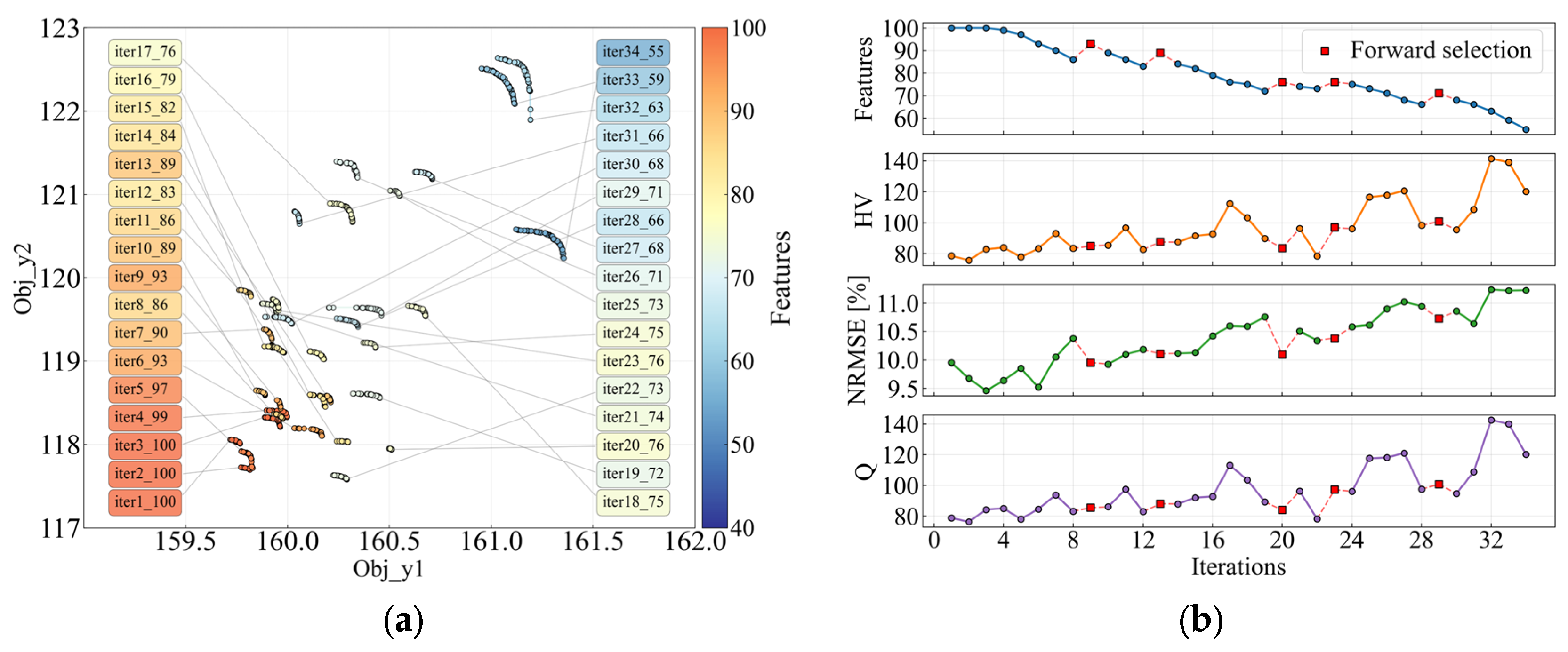
The generated dataset comprises 100 feature variables and two optimization objectives, with a total of 250 samples, which is comparable to the sample size of the investigated case in this paper. The synthetic dataset described above is utilized to validate the method proposed in this paper. The optimization objectives are to maximize Obj_y1 and Obj_y2. The algorithm parameters are configured as follows: the population size is 150, the number of generations is 100, the penalty factor is $k=2$, the weight coefficients are $w_1=0.3$ and $w_2=0.7$, and the amplification coefficient is $\lambda =0.5$. The results are presented in Figure 6. Figure 6a illustrates the evolution of the Pareto front over iterations, where differently colored points represent Pareto fronts at different iterations, and the color indicates the number of features used in the current iteration. Figure 6b shows the evolution trends of the metric parameters with iterations. As iterations proceed, the number of features gradually decreases, and the Pareto front shifts toward the upper right, indicating a steady improvement in optimization performance. When the decrease in Q exceeds the preset threshold, forward selection is triggered. Accordingly, the number of features increases, and the Pareto front quality improves, confirming the effectiveness of forward selection. When the number of features decreases to 63, all 60 key features are included; at this point, Q reaches its peak, and the Pareto front achieves its optimal. However, if this process continues and the number of features becomes less than 60, the Pareto front quality continues to deteriorate. This behavior aligns with the intrinsic characteristics of the dataset, thereby validating the accuracy and reliability of the proposed method.

4. Results and Analyses

4.1. Sampling and Numerical Results

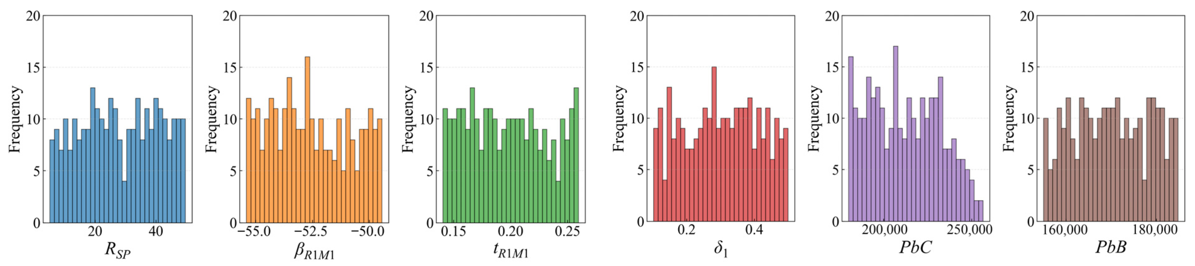
LHS is employed to sample the features listed in Table 2. The sampling range of geometric parameters is set to ±30% of the baseline design, while the sampling ranges for both the front fan and rear fan tip clearances are 0.1–0.5 mm. The operating condition parameters cover the full operating envelope of the ACF: the sampling range of the core outlet back pressure is 175–260 kPa, and that of the bypass outlet back pressure is 155–185 kPa. Representative sampling results are shown in Figure 7. Although all sample points cover their respective parameter ranges, some features are not perfectly uniformly distributed. For instance, the number of samples at high PbC values is relatively small because high PbC tends to induce flow instability and results in numerical non-convergence. Ultimately, 284 valid samples are obtained, which is more than twice the number of features (119), meeting the LHS requirement and providing reliable support for subsequent modeling and optimization analysis.

In this study, the CFD simulations are performed using 64 cores in parallel on an AMD EPYC 7742 platform. The wall-clock time required to generate the 284 initial samples is approximately 150 h. Based on this dataset, the total algorithmic overhead—including training the neural network models, calculating SHAP values, and executing the MOO iterations—takes only about 2 h. In contrast, a standard genetic algorithm running directly in the full 119-dimensional feature space typically requires thousands of expensive CFD evaluations to converge. Therefore, although the proposed method introduces a slight overhead for machine learning modeling at each iteration, this minimal cost is completely offset by the massive reduction in CFD simulations, ultimately saving over 80% of the total computational time.

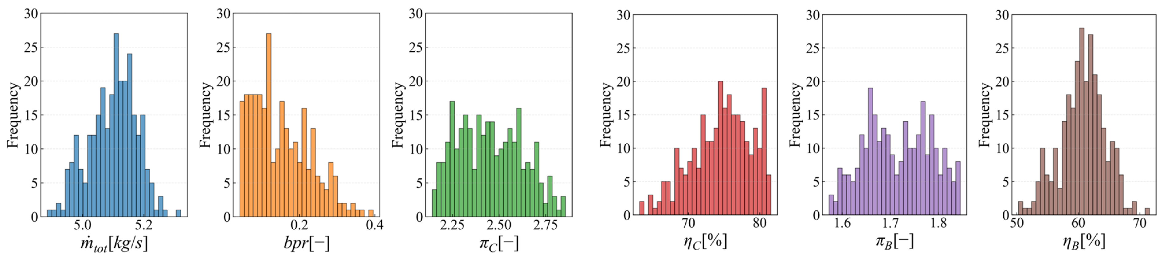
The performance distributions of all sample points are obtained by CFD simulations, as shown in Figure 8. These include a total of six parameters: total mass flow ${\dot{m}}_{tot}$, bypass ratio $bpr$, core pressure ratio ${\pi }_C$, core efficiency ${\eta }_C$, bypass pressure ratio ${\pi }_B$, and bypass efficiency ${\eta }_B$. While some performance parameters exhibit similar distribution trends, others show different trends, indicating that different features and their combinations influence ACF performance through significantly different mechanisms.

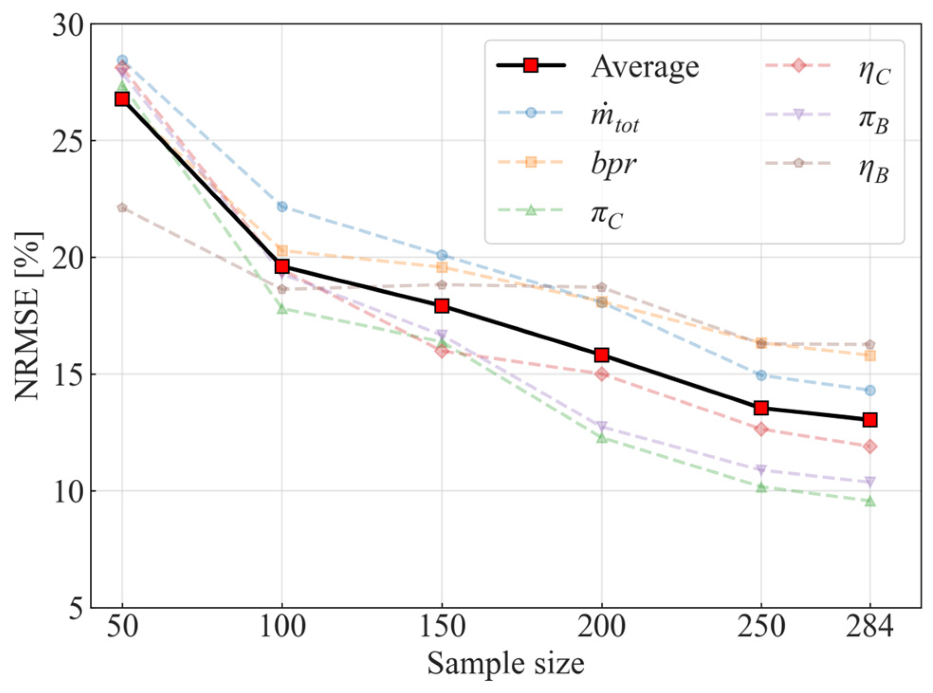
To evaluate the dataset’s sufficiency and the convergence characteristics of the initial surrogate model, Figure 9 illustrates the variation in the neural network surrogate model’s prediction error with respect to the sample size in the initial 119-dimensional features. In the figure, the solid black line represents the average NRMSE across the six performance parameters, while the dashed lines denote each individual performance parameter. As shown in the figure, when the sample size increases from 50 to 150, the average prediction error exhibits a significant downward trend. However, when the sample size surpasses 200 and approaches 284, the error decline significantly slows down, indicating that the surrogate model has transitioned into a phase of clearly diminishing marginal returns. At this stage, continuing to increase the sample size would require a massive number of samples to gain only a marginal improvement in accuracy. Given the prohibitive time cost of CFD simulations for sample acquisition, such an approach is highly uneconomical from an engineering perspective. Therefore, the current 284 initial samples strike an optimal trade-off between fulfilling the surrogate modeling requirements of the neural network and controlling the overall computational cost, satisfying the requirements of this study.

4.2. Iterative Process Analysis

For the ACF investigated in this paper, the optimization objectives are to maximize both the core pressure ratio and core efficiency, while ensuring that total mass flow, bypass ratio, and bypass pressure ratio remain within prescribed constraint ranges to satisfy overall engine matching requirements. In addition, two operating condition parameters are fixed: the core outlet back pressure is 240 kPa, and the bypass outlet back pressure is 170 kPa. Furthermore, to ensure structural reliability, the front fan and rear fan tip clearances are set to 0.3 mm. Thus, the optimization problem can be expressed as follows:

$$\begin{array}{l}\left\{\begin{array}{c}\max {\pi }_{\mathrm{C}}\\ \max {\eta }_C\end{array}\right.\\ s.t. 5.05<{\dot{m}}_{tot}<5.15 \mathrm{kg}/\mathrm{s}\\ \hspace{0.33em}\hspace{0.33em}\hspace{0.33em}\hspace{0.33em}\hspace{0.33em}\hspace{0.33em}0.08<bpr<0.12\\ \hspace{0.33em}\hspace{0.33em}\hspace{0.33em}\hspace{0.33em}\hspace{0.33em}\hspace{0.33em}1.7<{\pi }_B<1.9\\ \hspace{0.33em}\hspace{0.33em}\hspace{0.33em}\hspace{0.33em}\hspace{0.33em}\hspace{0.33em}\mathrm{PbC}=240 \mathrm{kPa}, \mathrm{PbB}=170 \mathrm{kPa}\\ \hspace{0.33em}\hspace{0.33em}\hspace{0.33em}\hspace{0.33em}\hspace{0.33em}\hspace{0.33em}{\delta }_1=0.3 \mathrm{mm}, {\delta }_2=0.3 \mathrm{mm}\end{array}$$

(10)

Figure 9. Convergence of surrogate model prediction error with increasing sample size in the initial 119-dimensional features.

Figure 9. Convergence of surrogate model prediction error with increasing sample size in the initial 119-dimensional features.

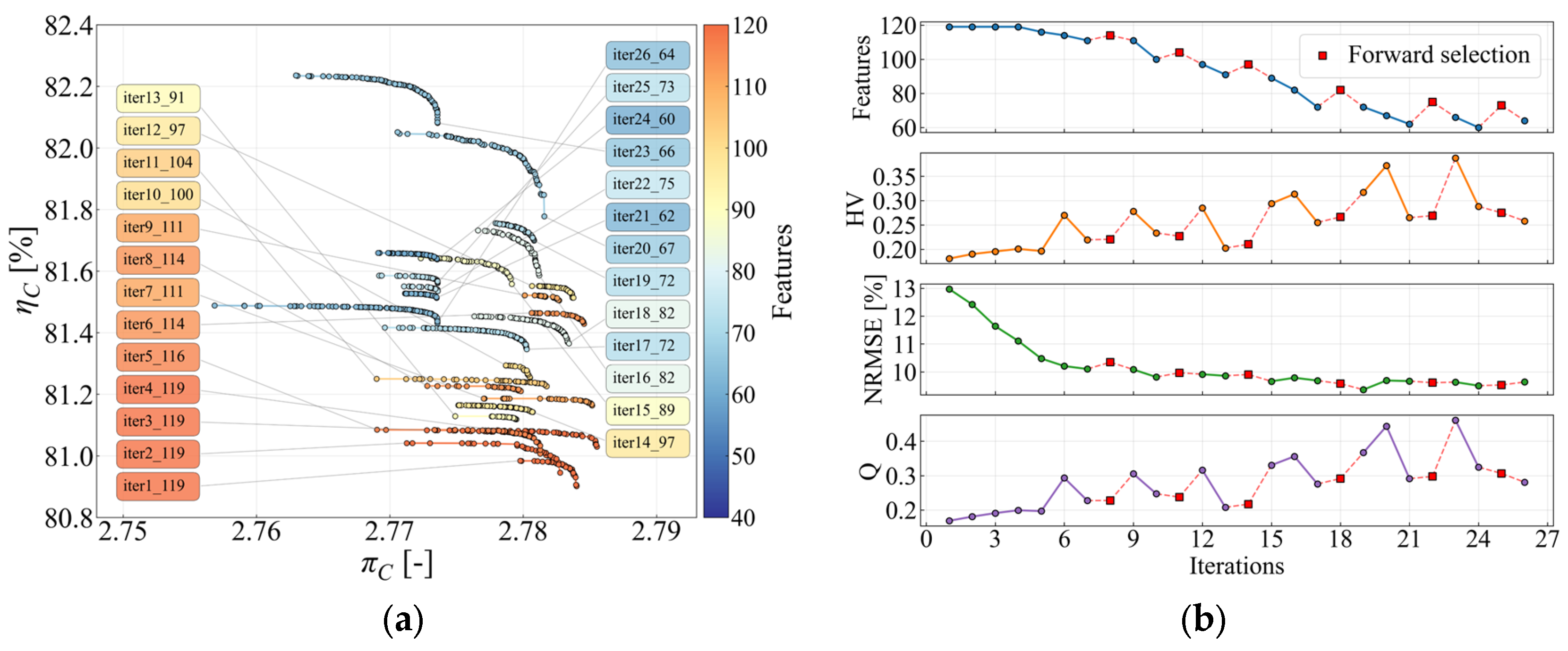
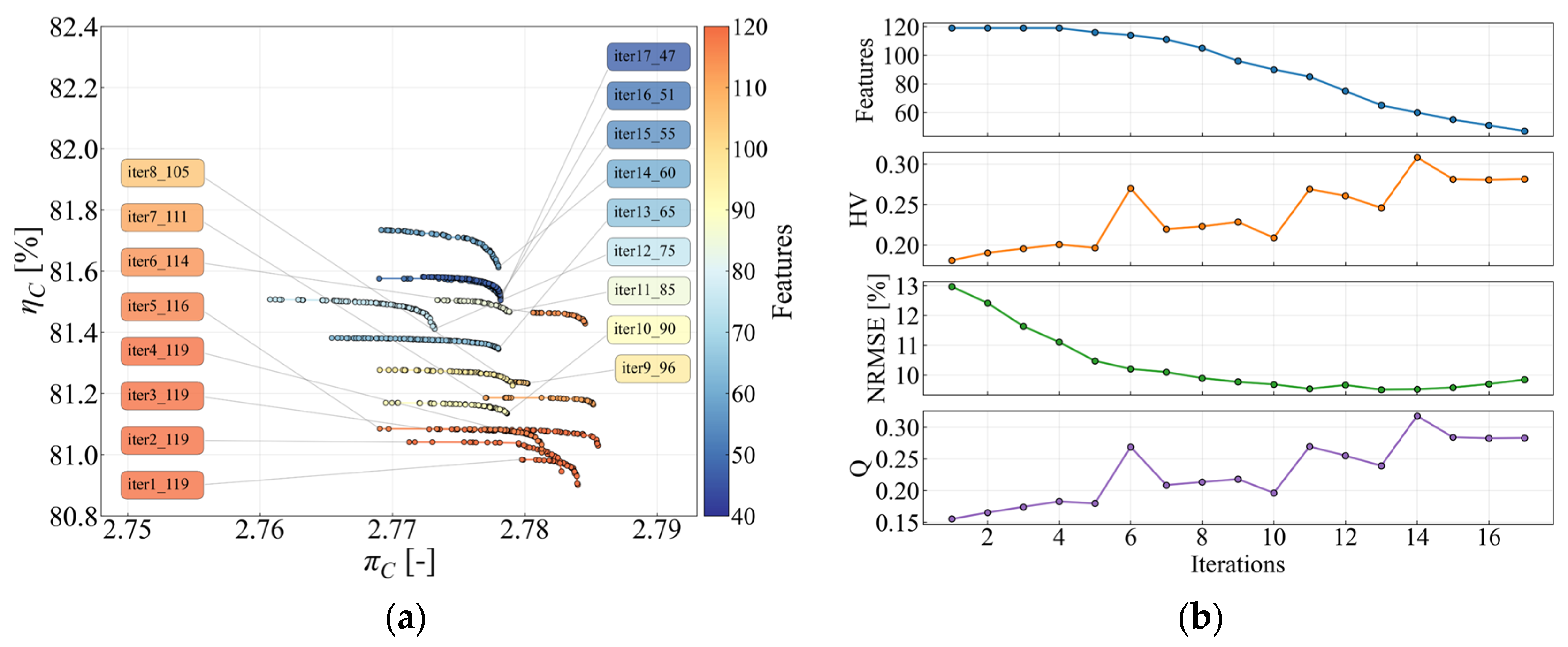
During optimization, the algorithm parameters are configured as follows: the population size is 150, the number of generations is 100, the penalty factor is $k=2$, the weight coefficients are $w_1=0.3$ and $w_2=0.7$, and the amplification coefficient is $\lambda =0.5$. The results are presented in Figure 10. As iterations proceed, the number of features decreases from the initial 119 to a range of 60–80. The NRMSE drops rapidly and then stabilizes, indicating that feature selection effectively eliminates low-sensitivity redundant features, thereby enhancing the generalization capability and prediction accuracy of the neural network model. The HV metric exhibits an overall increasing trend with stage-wise fluctuations and finally stabilizes at a high level, indicating improvements in both the convergence and diversity of the Pareto front. Specifically, the Pareto front gradually migrates from a relatively low efficiency region toward a high efficiency region, and a higher efficiency branch forms in the mid-to-late stages, reflecting the guiding effect of the weight coefficients and amplification coefficient on the preference for optimization objectives. The overall trend of Q is largely consistent with that of HV. When Q decreases beyond a preset threshold, forward selection is triggered; subsequently, Q rebounds as the feature count is moderately increased, and the quality of the Pareto front further improves. This observation reflects the process of gradually approaching the global optimum through dynamic adjustment of the feature space. At iteration 23, Q reaches its maximum with 66 features. If the number of features is further reduced, Q continues to decrease, and even forward selection fails to restore performance, indicating that the current feature subset and optimization results are near the global optimum. Ultimately, the core efficiency increases from 80.98% in the initial iterations to 82.24%, while the core pressure ratio remains within a stable range.

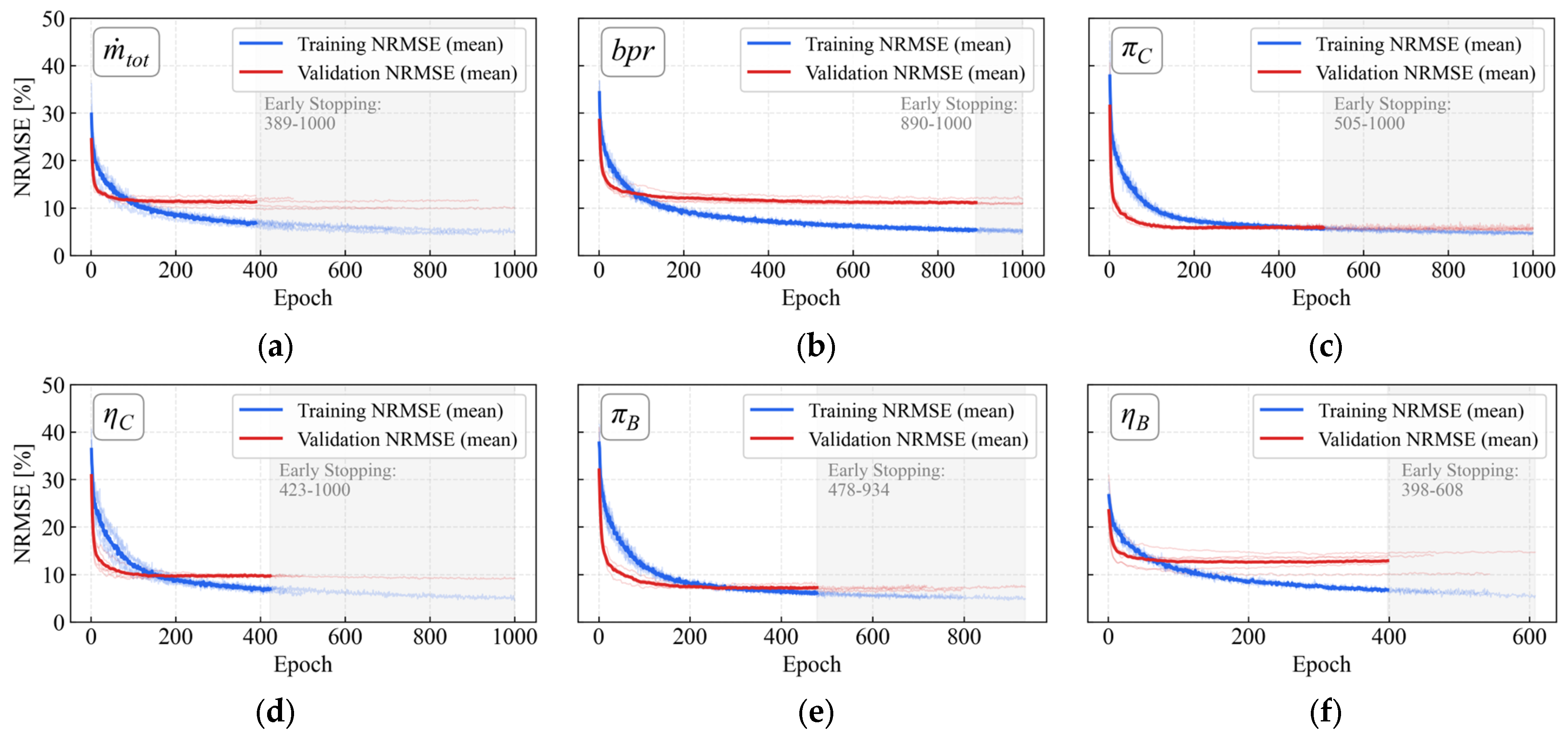
To evaluate the generalization capability of the surrogate models, Figure 11 presents the learning curves for the six performance parameters at iteration 23. The bold lines denote the mean errors across the 5-fold cross-validation, while the faint lines represent the independent results of each fold. The training errors (blue curves) and validation errors (red curves) exhibit a steady decrease during the initial training phase before stabilizing into a plateau, with no divergence or upward trend observed as training progresses. This stable convergence, coupled with the early stopping mechanism (denoted by the shaded regions), indicates that the surrogate models achieve reliable generalization and avoid overfitting under the current sample-to-feature ratio. Furthermore, the neural network architecture (64 × 64 neurons) is kept constant during the iterative feature selection to serve as a controlled variable, isolating the impact of dimensionality reduction from hyperparameter tuning. Although the input dimension decreases from 119 to 66, the risk of capacity mismatch and over-parameterization is mitigated by regularization strategies, specifically a dropout rate of 0.3 and a weight decay coefficient of 0.0001. The convergence trend in Figure 11 indicates that the network’s effective capacity is properly regulated as input dimension changes, suggesting that the elimination of redundant features and noise is a primary driver for the improvements in both surrogate model accuracy and Pareto front quality. However, it should be noted that keeping a fixed neural network architecture introduces potential coupled effects. As the input dimensionality decreases substantially, the effective representational behavior and capacity of the fixed-size network may alter. Future research could explore adaptive network architectures that dynamically scale with input dimensionality to increase the robustness of the optimization results.

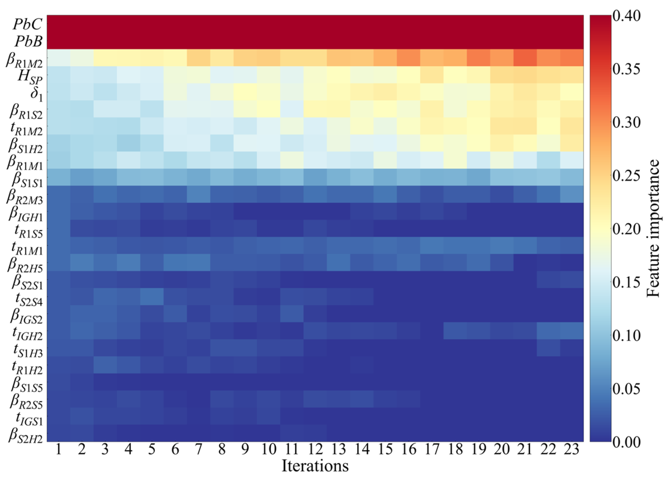
Figure 12 illustrates the heatmap of feature importance evolution. The horizontal axis denotes the iteration number, while the vertical axis denotes the features (ranked according to their importance in the first iteration). For clarity, 25 representative features are selected, including the top 10 features, 5 mid-ranked features, and the bottom 10 features. The color indicates feature importance, defined as the sum of feature importance ${\overline{\varphi }}_i$ over the six performance parameters, reflecting the overall influence of each feature on the integrated performance of ACF. PbC and PbB remain dark red throughout all iterations, indicating that outlet boundary conditions are the most critical factors determining the ACF performance. This trend is consistent with the physical principle that operating points vary significantly with back pressure. For other geometric features, as feature selection proceeds, the importance of higher-ranked features gradually increases while the importance of lower-ranked features continuously decreases until they are eliminated. This trend is visualized by the upper-right region transitioning toward red and the lower-right region converging toward blue. Notably, specific features are reintroduced into the feature space through forward selection and ultimately retained in the optimal subset: $t_{IGH2}$ at iteration 18, ${\beta }_{S2S1}$ and $t_{S1H3}$ at iteration 22. This phenomenon occurs because, in early iterations, the accuracy of the neural network model is relatively low and cannot accurately capture the effects of certain features, potentially leading to the erroneous elimination of key features. Forward selection enables the recovery of such features, effectively preventing the accidental elimination of key features and enhancing the global search capability.

4.3. Composition and Regional Distribution of Optimal Features

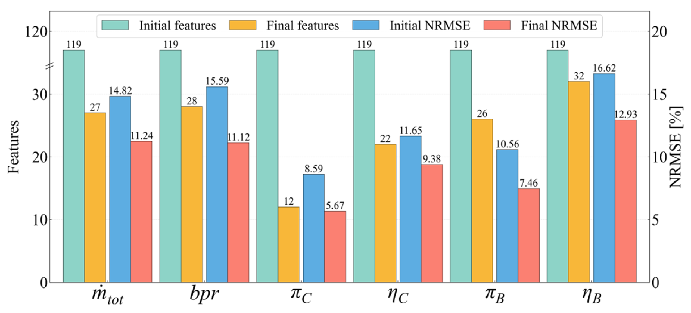
According to the above analysis, the optimal feature subset contains 66 features. To further elucidate the composition of this subset, Figure 13 compares the number of features and model accuracy for each performance parameter. All performance parameters show a substantial reduction in feature number from the initial 119; specifically, after feature selection, the number of features for ${\dot{m}}_{tot}$, $bpr$, ${\pi }_C$, ${\eta }_C$, ${\pi }_B$ and ${\eta }_B$ decrease to 27, 28, 12, 22, 26, and 32, respectively. Meanwhile, the prediction error is significantly reduced, with the average NRMSE decreasing from 13% initially to 9.6% finally. These results indicate that significant dimensionality reduction not only retains key information but also markedly improves surrogate model accuracy and generalization, confirming that the original design space contains a large number of redundant features and noise. This also demonstrates that the XAI-driven feature-selection strategy proposed in this paper can improve surrogate model performance while significantly compressing feature dimensionality, achieving synergistic optimization of “dimension reduction” and “performance enhancement.”

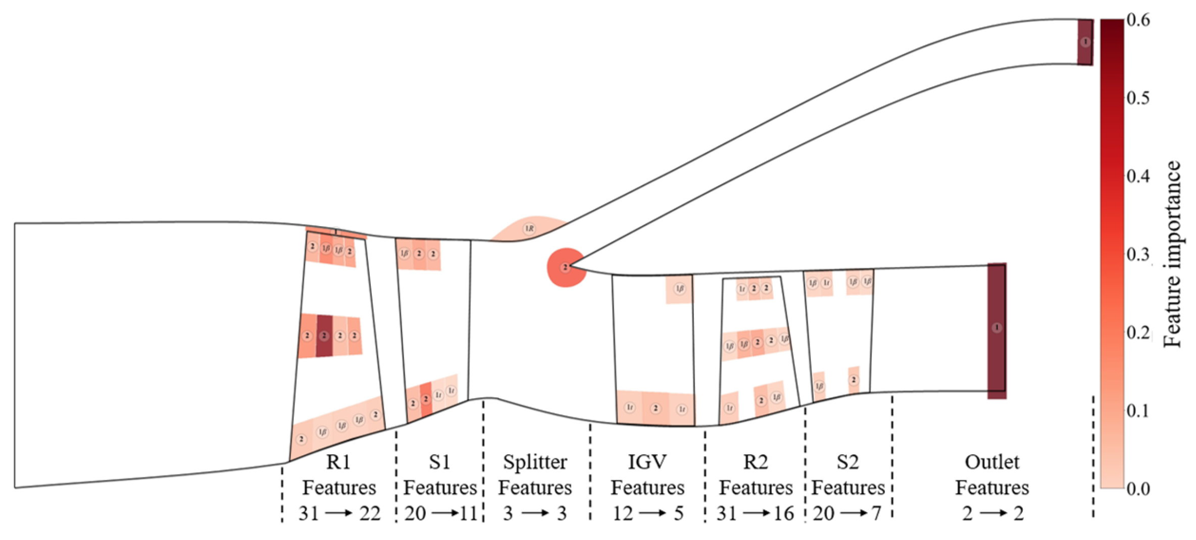
Figure 14 illustrates the distribution of the optimal features in the meridional section. Color intensity represents feature importance, and both the original and optimal numbers of features in each region are annotated. The numerical values in the colored regions denote the number of features, where $t$ represents thickness and $\beta$ represents angle. Different regions exhibit significantly different sensitivities regarding performance, among which the outlet boundary conditions, features in the R1 mid-span region, and splitter position features show the highest sensitivity. A comparison of feature retention ratios across components reveals that rotor components retain a significantly higher proportion of features than stator components, and upstream components retain more than downstream components. The results indicates that upstream components, characterized by higher work capacity and upstream positioning, contribute more critically to the ACF performance and are therefore the core regions of concern in design optimization.

4.4. Sensitivity Analysis

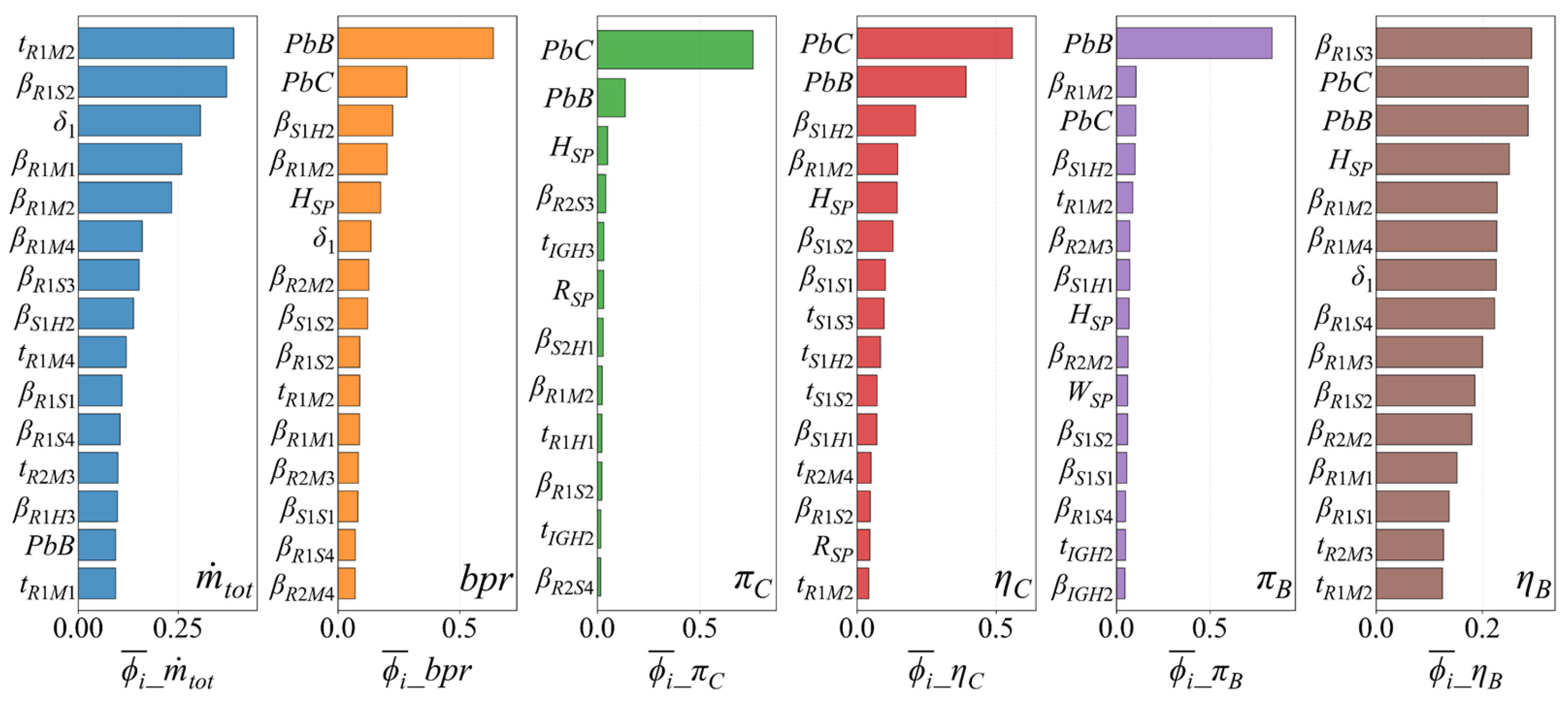
To analyze the importance of different features regarding the performance parameters, Figure 15 presents the feature importance ${\overline{\varphi }}_i$ corresponding to each performance parameter. For clarity, only the top 15 features are shown. The results indicate that the impacts of features on performance parameters differ significantly: regarding the prediction of $bpr$, ${\pi }_C$ and ${\pi }_B$, the features PbB and PbC clearly dominate, implying that operating boundary conditions strongly constrain bypass matching and pressure ratio characteristics; whereas for ${\dot{m}}_{tot}$, ${\eta }_C$ and ${\eta }_B$, geometric features are also prominent, indicating that flowpath geometry plays a key role in determining mass flow and efficiency. Further analysis shows that the feature sets for different performance parameters comprise both shared features and parameter-specific features. However, even for shared features, their importance differs. For example, although ${\beta }_{R1M2}$ is selected for all six performance parameters, its feature importance ${\bar{\varphi }}_i$ differs markedly among them, suggesting that the underlying mechanisms by which this feature affects each performance parameter are distinct.

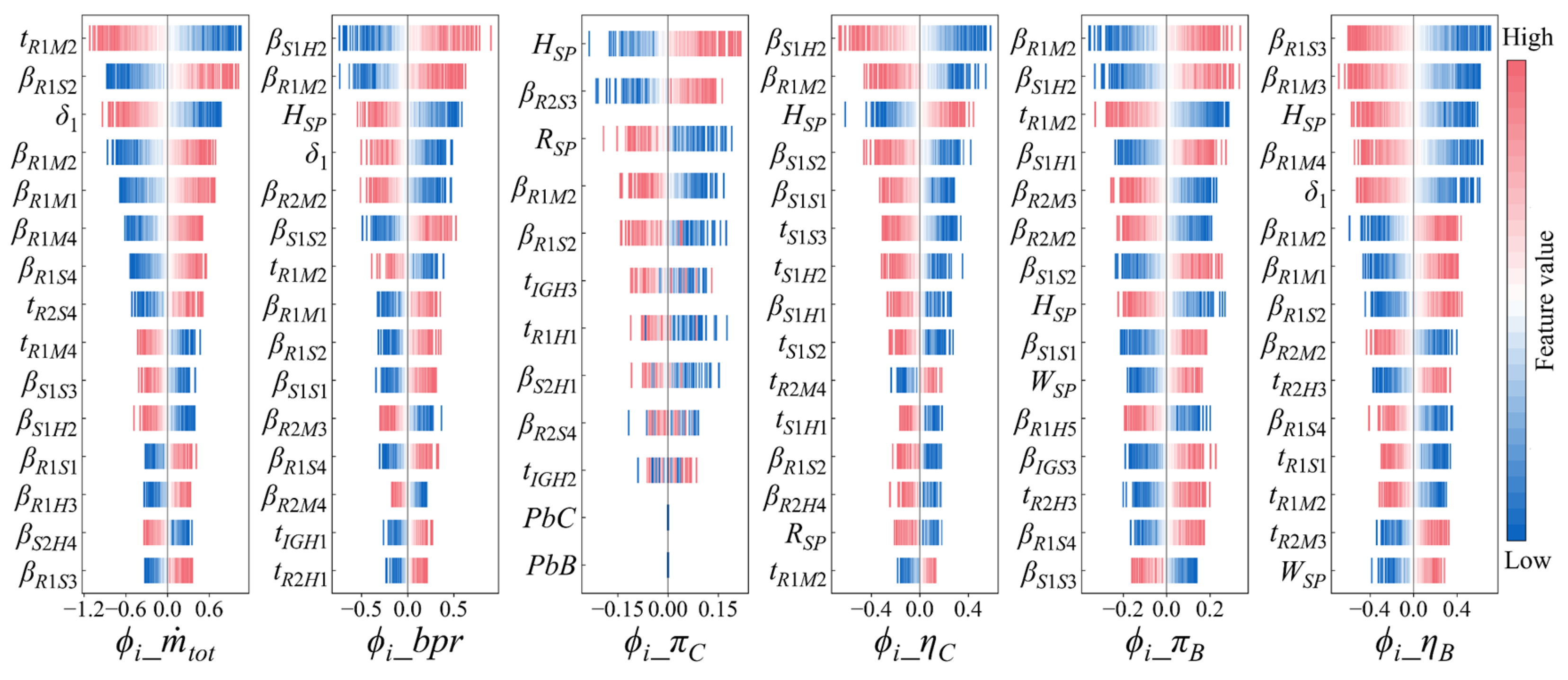
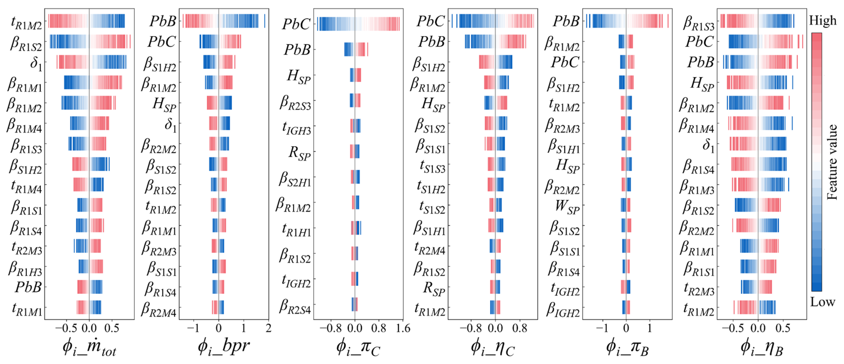
Figure 16 and Figure 17 illustrate the distributions of Shapley values for features under varying and fixed operating conditions, respectively. In the varying condition case, the original back pressure ranges are utilized, meaning distinct samples possess different back pressure conditions. Conversely, in the fixed condition case, PbB and PbC are fixed at 170 kPa and 240 kPa, respectively; Shapley values are recalculated under these settings to eliminate the impact of operating condition variations on the interpretability analysis. The horizontal axis represents the Shapley value ${\varphi }_i$, denoting the marginal contribution of a feature to performance prediction, while the vertical axis represents the features. The color gradient shifts from blue to red as the feature value increases. Specifically, if ${\varphi }_i$ tends to increase simultaneously with the feature value, a positive correlation exists with the performance parameter; otherwise, a negative correlation is indicated. Most of the features exhibit clear monotonic correlations with the performance parameters. Features with greater influence display a noticeably wider range of ${\varphi }_i$, indicating a larger contribution magnitude and higher sensitivity; this is consistent with the importance ranking in Figure 15. For instance, regarding ${\beta }_{R1M2}$: as it increases, ${\dot{m}}_{tot}$, $bpr$, ${\pi }_B$ and ${\eta }_B$ increase, whereas ${\pi }_C$ and ${\eta }_C$ decrease. Therefore, trade-offs are required during optimization to identify the optimal design. When the operating condition is fixed, the importance ranking changes slightly, but the influence patterns remain consistent with those under varying operating conditions. This indicates that optimization performed under fixed operating conditions remains valid across the full operating envelope, thereby validating the strategy adopted in this paper.

4.5. Verification of Forward Selection Effectiveness

To verify the effectiveness of forward selection, comparative results without this strategy are provided in Figure 18. Compared with the strategy utilizing forward selection, the number of iterations is significantly smaller, and the feature count decreases monotonically throughout the process. Nevertheless, the overall evolutionary trends of the Pareto front and metric parameters are similar to those observed with forward selection: the quality of the Pareto front improves during iterations until the number of features becomes excessively small, after which performance degrades and subsequently stabilizes. Metric Q exhibits an overall pattern of steadily increasing, then decreasing, and finally stabilizing, reaching its peak at iteration 14 with 60 features. In the corresponding optimization results, the maximum core efficiency is 81.73%, which is significantly lower than the 82.24% obtained with forward selection. This indicates that without forward selection, the algorithm is more prone to becoming trapped in local optima.

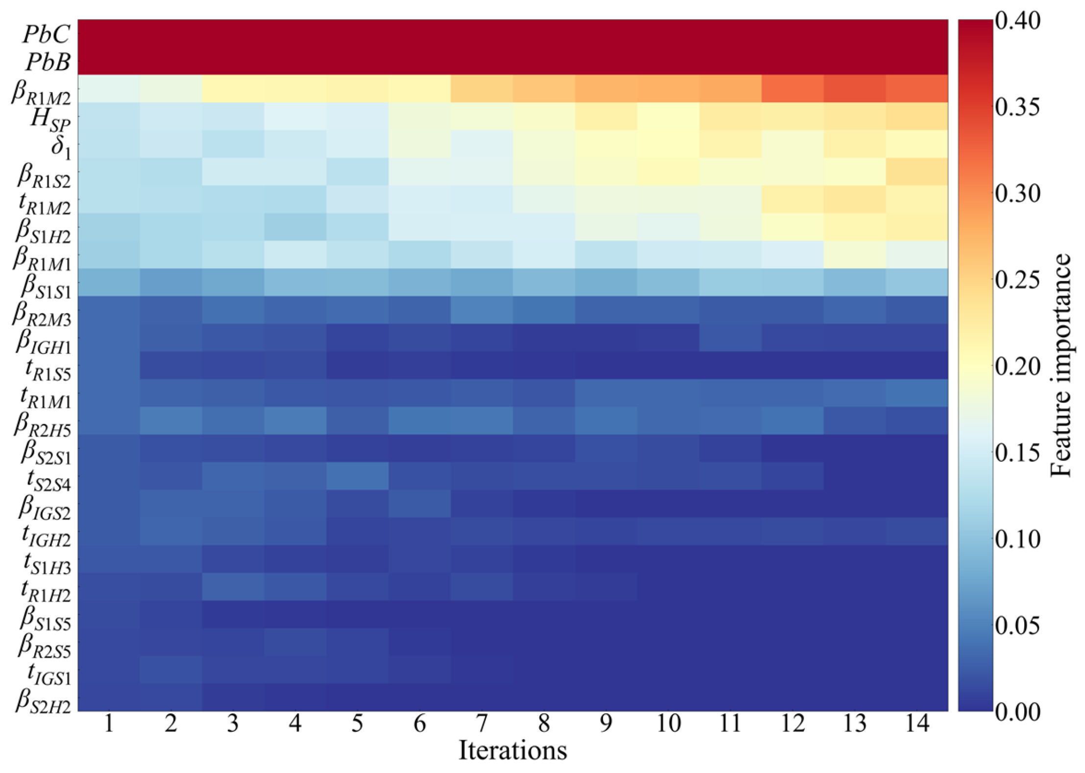
To analyze the causes of the performance difference, Figure 19 presents the heatmap of feature importance evolution without forward selection, using the same feature set as shown in Figure 12. The overall evolution pattern of feature importance remains consistent: the importance of higher-ranked features gradually increases with iterations (the upper-right region transitions from light colors to red), while that of lower-ranked features continuously decreases until elimination (the lower-right region converges toward blue). However, without the “feature expansion” mechanism of forward selection, once a feature is eliminated, it cannot be reintroduced. This leads to the permanent exclusion of certain key features with potential global contributions (e.g., ${\beta }_{S2S1}$ and $t_{S1H3}$) from the optimal feature subset. This irreversible elimination is the fundamental reason for the performance difference. It also explains mechanistically that forward selection can effectively avoid erroneous elimination of key features, thereby improving the global optimality of the feature subset and raising the upper bound of the final optimization quality.

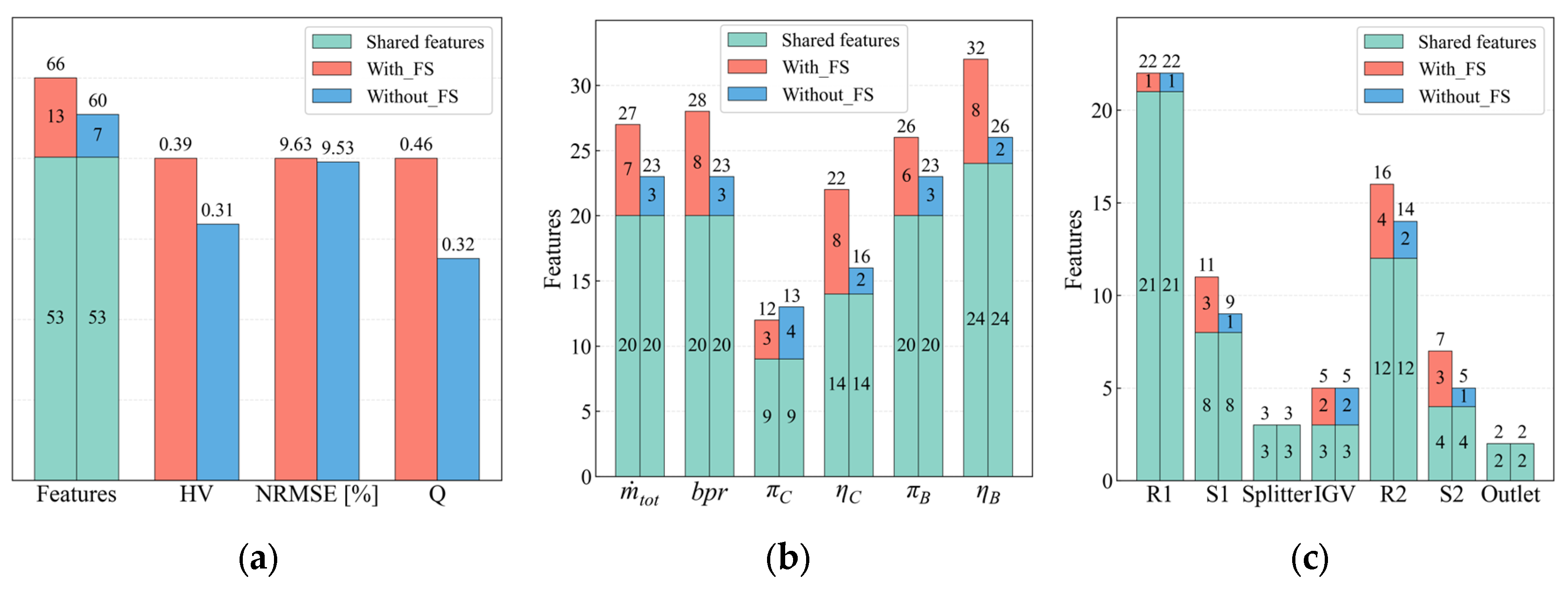
Figure 20 compares the composition of feature subsets and optimization performance between the strategies with and without forward selection. In the figure, green indicates features shared by both strategies, red indicates those associated with the strategy with forward selection, and blue indicates those with the strategy without forward selection. As shown in Figure 20a, the two methods ultimately retain 60 and 66 features, respectively, including 53 shared features. Although the NRMSE is similar for both strategies, HV increases significantly from 0.31 to 0.39 when forward selection is adopted, leading to an increase in Q from 0.32 to 0.46. This indicates that forward selection improves the overall optimization performance primarily by enhancing the distribution quality of the Pareto front. Figure 20b compares feature selection results for different performance parameters. With forward selection, the number of features increases noticeably; specifically, for the optimization objective ${\eta }_c$, the feature count increases from 16 to 22, which has a significant impact on improving optimization quality. Figure 20c shows that both strategies retain nearly the same features in the R1, Splitter, and Outlet regions, while the differences are mainly concentrated in the S1, R2, and S2 regions. From a spatial distribution perspective, this demonstrates that forward selection can effectively capture features with potential contributions to performance and serves as a key step in improving global search capability and final optimization quality.

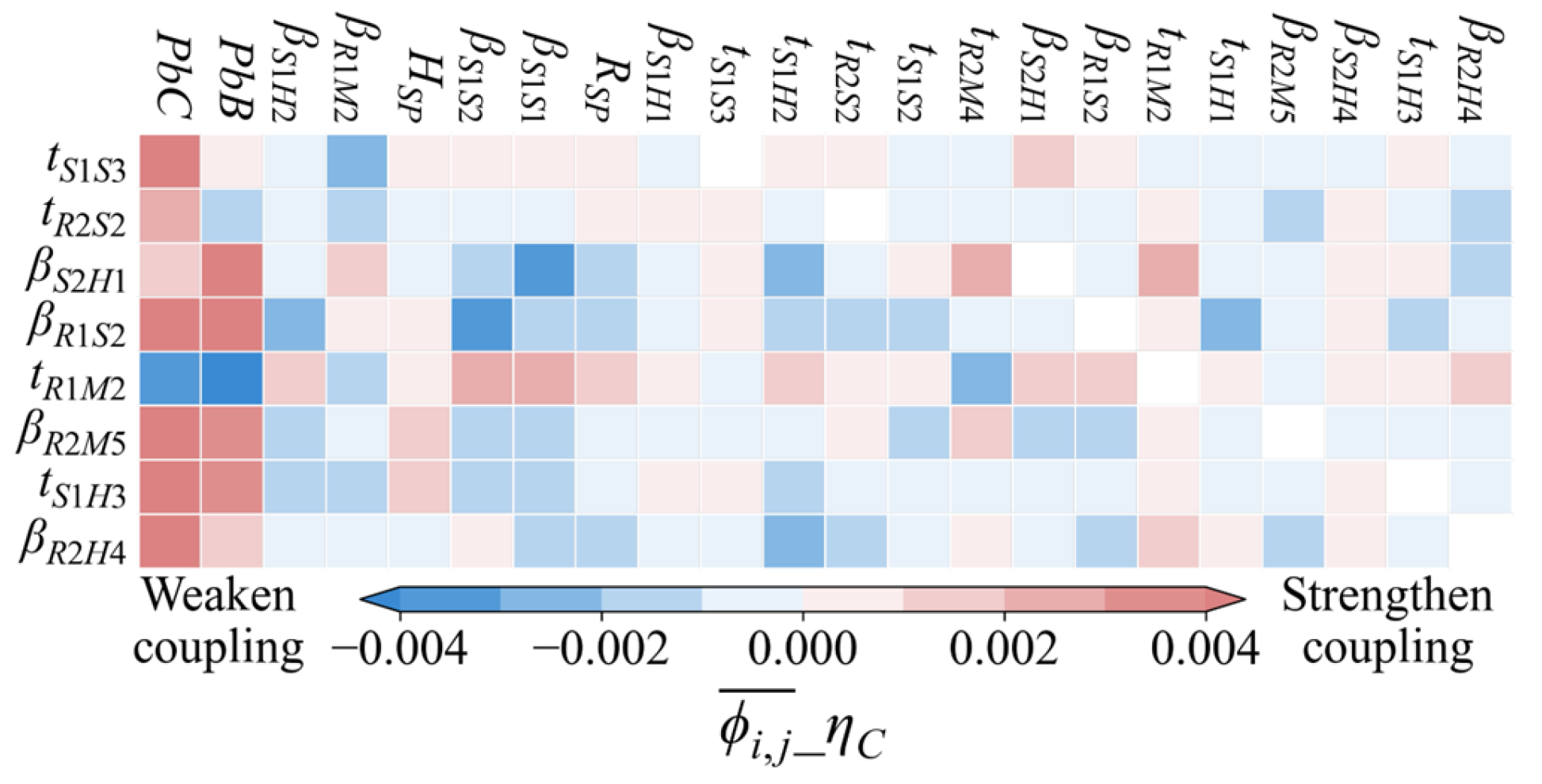
Figure 21 shows the heatmap of the coupling effects of features on core efficiency when forward selection is employed. The left vertical axis lists the eight unique features for core efficiency identified with forward selection in Figure 20b, while the top horizontal axis lists all 22 optimal features. The color intensity denotes the SHAP coupling effect value ${\varphi }_{i,j}$: red indicates a strengthening coupling effect, and blue indicates a weakening coupling effect. These eight unique features exhibit significant coupling effects with the operating condition features (PbC and PbB) and other geometric features ($H_{SP}$, ${\beta }_{S1S2}$, $t_{R1M2}$, etc.). Taking $t_{S1H3}$ as an example, it shows a significant strengthening coupling effect with PbC, PbB, and $H_{SP}$. As indicated in Figure 16 and Figure 17, PbC, PbB, and $H_{SP}$ show clear positive correlations with core efficiency. When $t_{S1H3}$ is reintroduced through forward selection, the positive effects of these features on core efficiency can be further amplified through coupling. This forms synergistic gains under certain feature coalitions, which is highly beneficial for improving core efficiency. Since the contributions of such features mainly manifest through coupling effects, without forward selection they can easily be misjudged as insignificant due to their low independent contributions in early iterations and thus be eliminated prematurely. Forward selection can effectively identify and retain these key coupled features, avoiding information loss, enhancing the surrogate model’s representation of nonlinear coupling, and improving global search capability.

4.6. Performance Comparison Between Baseline and Optimal Designs

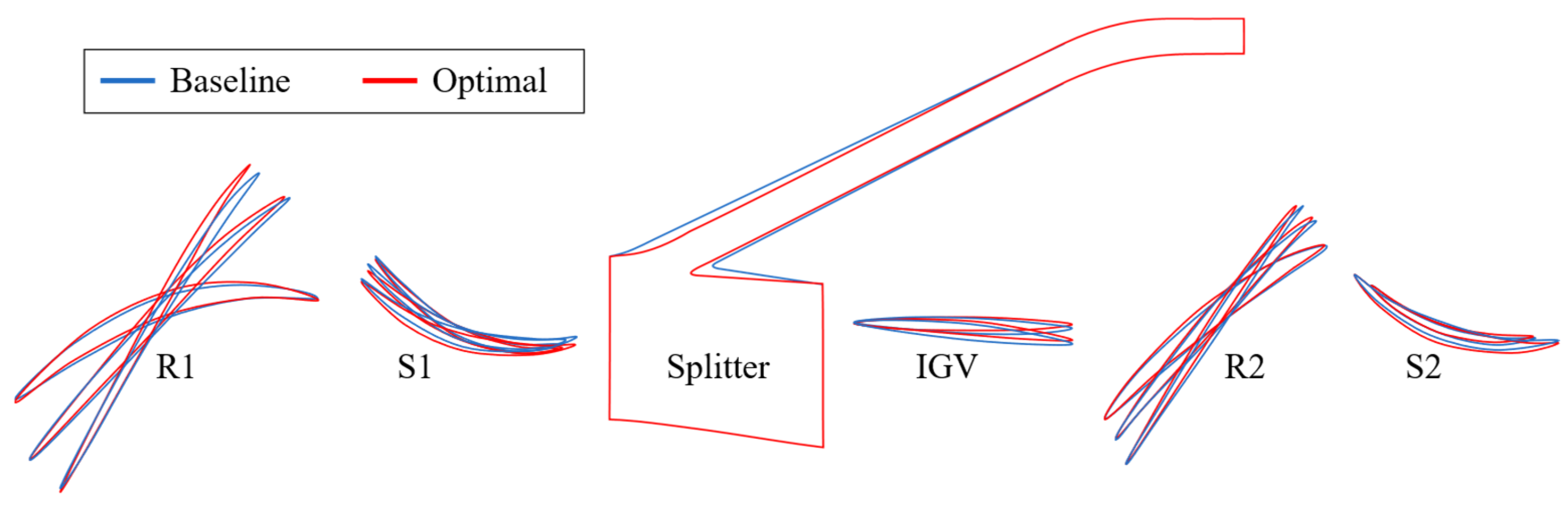
Based on the above MOO results, and considering structural strength, manufacturability, and machining constraints, the final optimal design of the ACF is determined. Figure 22 compares the geometries of the baseline and optimal designs, where blue represents the baseline and red represents the optimal design. It can be seen that the optimal features are mainly concentrated in key regions such as the R1 and R2 airfoils and the splitter position, which is manifested as the systematic re-profiling of multi-section airfoils and adjustments to the splitter location. These geometric changes are highly consistent with the regional distribution of optimal features shown in Figure 14, further verifying the effectiveness of the proposed feature selection and MOO method in identifying key features and guiding geometric modifications.

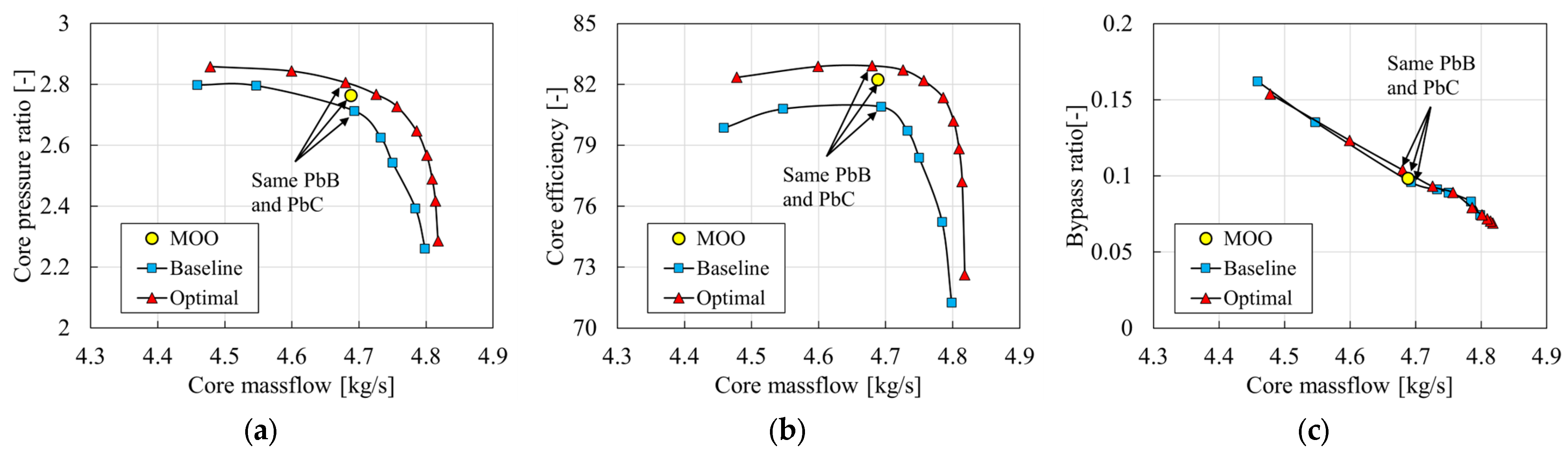
Figure 23 compares the performance of the baseline and optimal designs, including the core pressure ratio characteristic, core efficiency characteristic, and bypass ratio characteristic. Blue squares denote the baseline design, yellow circles denote the best MOO solution selected from Figure 10a, and red triangles denote the optimal design. Compared with the baseline, the core pressure ratio and core efficiency characteristics of the optimized design shift upward overall, while the bypass ratio characteristic remains almost the same. Under the same back pressure condition, the core pressure ratio increases from 2.71 to 2.81, and the core efficiency increases from 80.80% to 82.92%, indicating that optimization of the features effectively improves flow matching and reduces losses. In addition, the optimal design further improves performance relative to the MOO solution, mainly due to a rational redesign in the engineering design stage: considering structural strength and manufacturability constraints, expert design knowledge is incorporated to make targeted adjustments to geometric details, thereby achieving better comprehensive performance.

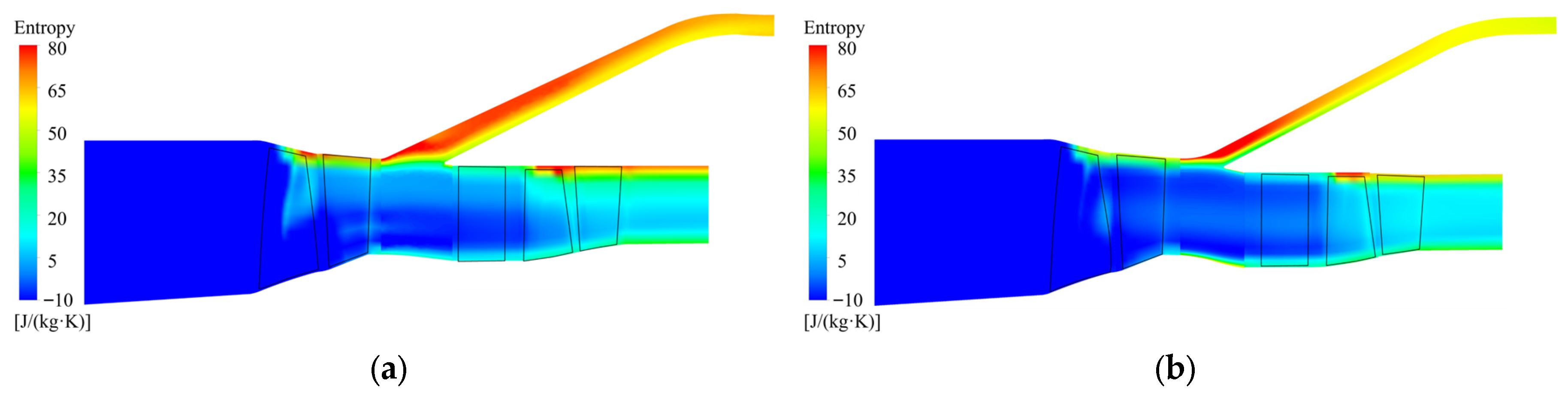
To further investigate the influence of the optimal design on the internal flow field, Figure 24 compares the meridional entropy distributions of the baseline and optimal designs. The optimal design exhibits significantly lower entropy levels in the mid-span, tip, splitter, and bypass regions. Furthermore, the extent of the high entropy region is notably diminished. This indicates that the optimal feature parameters effectively improve the flow organization within the blade passages while enhancing the matching between the core and bypass. This improvement in flow field suppresses flow separation and mixing, thereby significantly reducing flow losses.

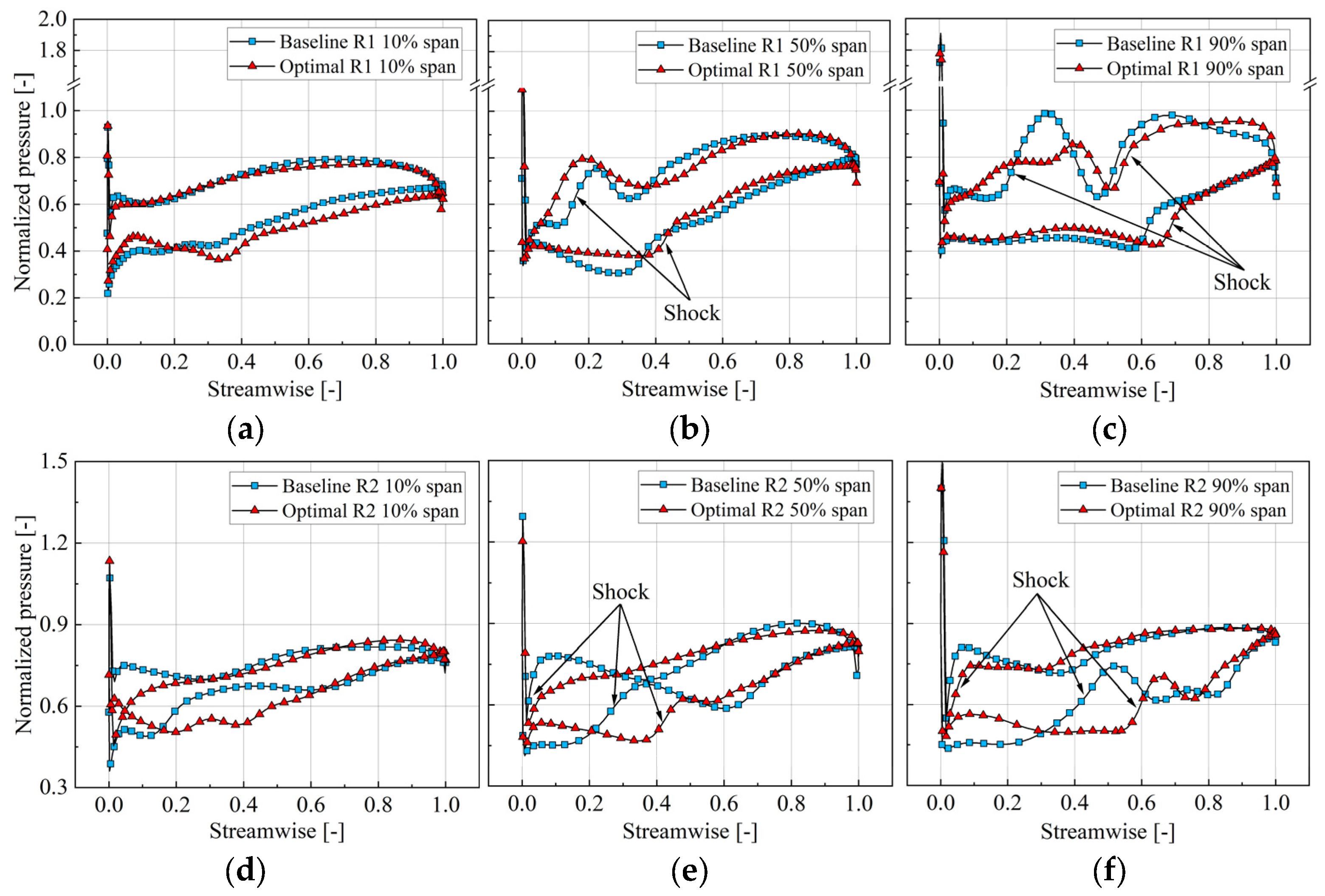
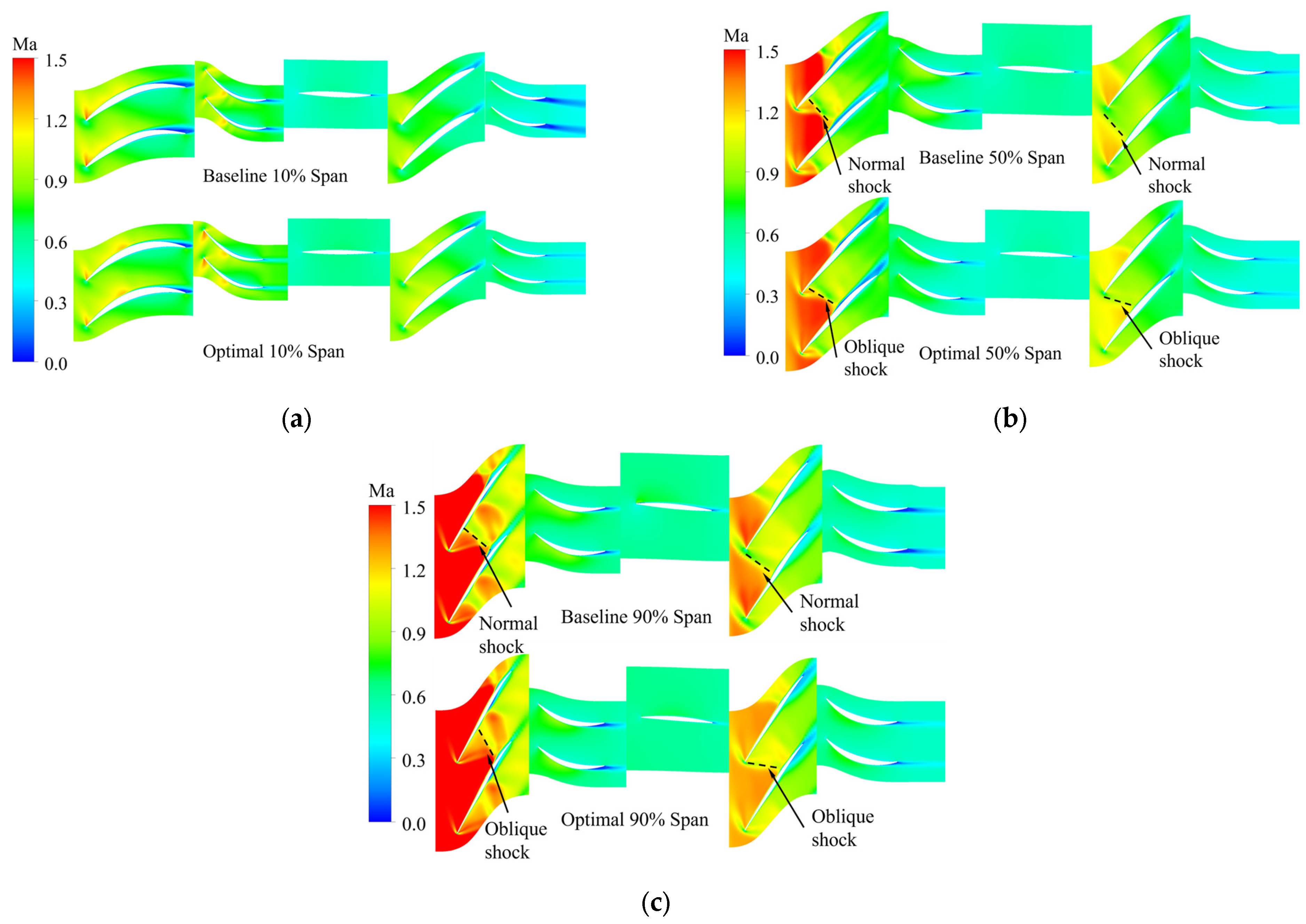
Figure 25 compares the Mach number contours at 10%, 50%, and 90% spans for the baseline and optimal designs. The optimal design significantly improves the shock structure within the passage and effectively suppresses flow separation. At 10% span, the flow is predominantly subsonic, and the optimized airfoil geometry achieves a better incidence match with the local flow field. Compared with the baseline, the wake width of the optimized blade becomes noticeably narrower, indicating that flow separation near the hub is effectively controlled and losses are significantly reduced. At 50% and 90% span, the flow is predominantly transonic. In the baseline design, strong normal shocks exist in both the R1 and R2 passages, leading to high shock losses and inducing severe boundary layer separation. In the optimal design, through the adjustment of airfoil angle and thickness distributions, the pre-shock Mach number is reduced, and the shock angle is altered; consequently, strong normal shocks are transformed into more efficient oblique shocks. This not only significantly reduces shock losses but also mitigates the shock–boundary layer interaction as well as the interaction between shocks and tip clearance leakage flow, thereby improving the efficiency. As indicated in Figure 16, the optimal feature subsets for R1 and R2 show high-density distributions in the mid-span and tip regions. This confirms that geometric features in these regions dominate the reconstruction of the shock structure and play a key role in the overall performance improvement.

Changes in blade loading further quantify and verify the improvement of the shock structure. As illustrated in Figure 26, compared with the baseline design, the optimal design exhibits a significant reduction in shock intensity and a downstream shift in the shock location. This downstream shift has two implications for the performance. In terms of stability, under throttled conditions, the reduced mass flow causes passage shocks to migrate toward the leading edge; once a shock becomes detached from the leading edge, stall may occur. By shifting the initial shock location downstream, the optimal design increases the distance available for the shock to travel upstream, thereby delaying shock spillage and enhancing the stable operating margin. In terms of efficiency, the downstream-shifted shock shortens the flow path length subjected to the post-shock adverse pressure gradient, thereby reducing the mixing losses induced by shock–boundary layer separation. Moreover, the optimal loading curve is smoother overall, and the adverse pressure gradient on the suction side is effectively alleviated, which delays boundary-layer thickening, suppresses flow separation, and further improves efficiency.

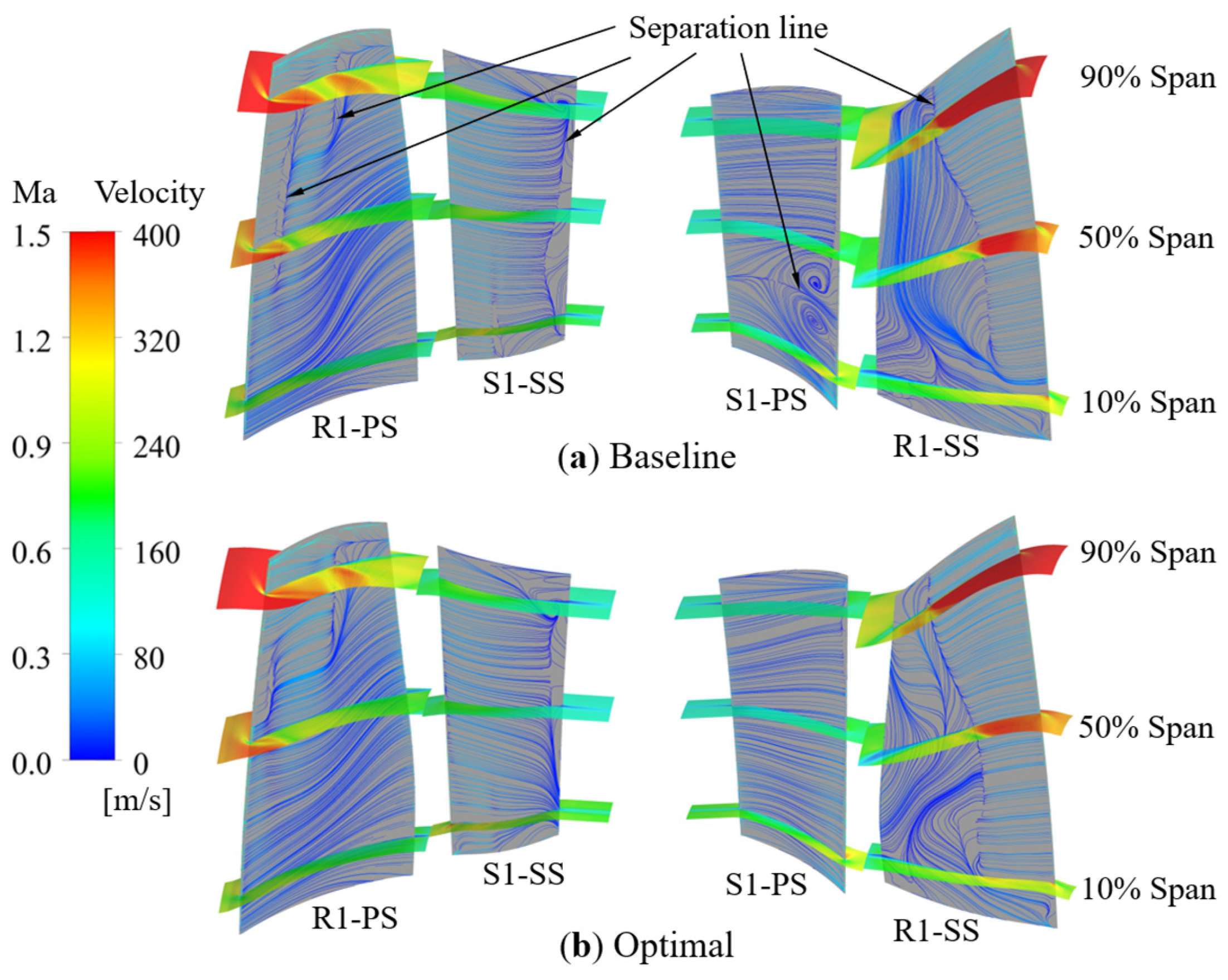
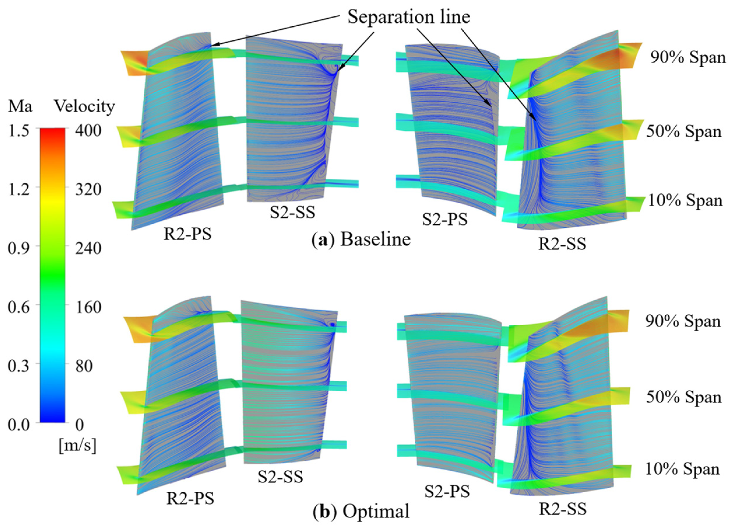
Figure 27 and Figure 28 compare the limiting streamline distributions on the blade surfaces of the front and rear fans for the baseline and optimal designs. In the baseline design, pronounced flow separation is observed on both the pressure and suction sides over the full span. Specifically, as indicated by the marked separation lines, the baseline rotors (R1 and R2) suffer from severe shock-induced boundary layer separation. The strong adverse pressure gradient generated by the passage shock forces the low-momentum fluid to accumulate and migrate radially toward the blade hub and tip. This intense radial migration exacerbates corner separation near the endwall regions, leading to severe aerodynamic blockage and mixing losses. In contrast, the optimal design exhibits fundamentally improved aerodynamic behavior. Driven by the refined airfoil angles and thickness distributions selected by the MOO method, the passage shock structure is reconstructed, which effectively mitigates the local adverse pressure gradient. Consequently, the onset of boundary layer separation on the suction sides is significantly delayed, and the spatial extent of the separated region is substantially reduced. The radial migration of corner secondary flows is effectively suppressed, allowing the boundary layer to remain attached over a larger portion of the blade chord. This enhanced flow attachment directly minimizes the wake width and reduces the associated mixing losses. Overall, the optimal design markedly enhances flow attachment on blade surfaces, improving overall flow field stability while reducing mixing losses.

Figure 26. Blade loadings of baseline and optimal designs: (a) R1 10% span; (b) R1 50% span; (c) R1 90% span; (d) R2 10% span; (e) R2 10% span; (f) R2 10% span.

Figure 26. Blade loadings of baseline and optimal designs: (a) R1 10% span; (b) R1 50% span; (c) R1 90% span; (d) R2 10% span; (e) R2 10% span; (f) R2 10% span.

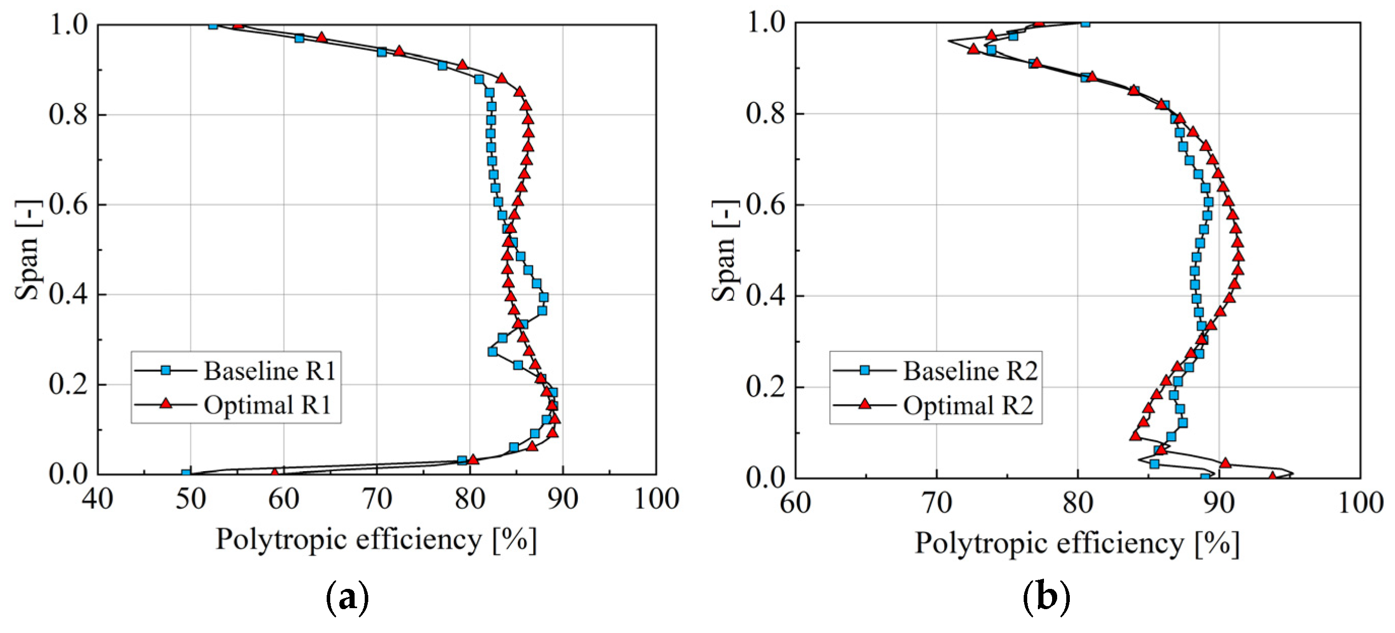
These localized flow field improvements are quantitatively reflected in the spanwise distribution of polytropic efficiency, as illustrated in Figure 29. For both R1 and R2, the optimal design achieves continuous efficiency gains over the majority of the blade span. Notably, the most significant improvements occur in the mid-span to tip regions (approximately 40% to 90% span for R1, and 20% to 80% span for R2). This distribution is highly consistent with the streamline analysis: the mitigation of shock-induced separation and the suppression of radial secondary flow migration primarily benefit the upper half of the blade passage. By confining the low-energy fluid and maintaining flow attachment, the optimized geometric features successfully translate microscopic aerodynamic corrections into macroscopic enhancements in overall rotor efficiency and flow stability.

Figure 27. Front fan limiting streamlines of baseline and optimal designs (PS: pressure side; SS: suction side): (a) Baseline design; (b) Optimal design.

Figure 27. Front fan limiting streamlines of baseline and optimal designs (PS: pressure side; SS: suction side): (a) Baseline design; (b) Optimal design.

Figure 28. Rear fan limiting streamlines of baseline and optimal designs (PS: pressure side; SS: suction side): (a) Baseline design; (b) Optimal design.

Figure 28. Rear fan limiting streamlines of baseline and optimal designs (PS: pressure side; SS: suction side): (a) Baseline design; (b) Optimal design.

Figure 29. Spanwise distribution of efficiency for baseline and optimal designs: (a) R1; (b) R2.

Figure 29. Spanwise distribution of efficiency for baseline and optimal designs: (a) R1; (b) R2.

5. Conclusions

To address the high-dimensional design optimization challenge for complex systems, this paper proposes a new MOO method and has been successfully applied to the design optimization of an ACF. The main conclusions are as follows:

• To deal with the tendency of traditional methods to become trapped in local optima within high-dimensional spaces, this paper proposes a new MOO method that integrates neural network surrogate model, SHAP analysis, and genetic algorithm. By comprehensively considering Pareto front quality, surrogate model accuracy, and optimization preference, a composite evaluation metric, Q, is defined as a feedback signal to guide the bidirectional feature selection based on SHAP analysis. This establishes a dynamic closed-loop process coupling feature selection with MOO, thereby significantly improving global search capability. Test results on a synthetic benchmark problem verify the accuracy and robustness of the method in handling high-dimensional nonlinear problems.
• Using the proposed method, an optimal feature subset of 66 features is accurately identified from 119 initial features, and a high-quality Pareto front is obtained. The spatial distribution of features indicates that upstream components, characterized by higher work capacity and upstream positioning, contribute more critically to the ACF performance and are therefore the core regions of concern in design optimization.
• Comparative results show that, without forward selection, the feature elimination is irreversible, leading to the premature exclusion of key features whose contributions manifest primarily through coupling effects. Forward selection can effectively capture the features with potential contributions to performance and plays a key role in improving global search capability and optimization quality, thereby validating the necessity of dynamically adjusting the feature space during optimization.
• Based on the MOO results, the final optimal design achieves synergistic improvements in pressure ratio and efficiency under structural strength and manufacturability constraints. Compared with the baseline design, under the same back pressure condition, the core pressure ratio increases from 2.71 to 2.81, and the core efficiency increases from 80.80% to 82.92%, while maintaining similar bypass ratio matching characteristics. Flow field analysis indicates that the performance gains mainly result from the reconstruction of the shock structure and the suppression of secondary flows, which effectively mitigates the losses from shock–boundary layer interaction and flow mixing. In addition, the regions with significant flow field improvements are highly consistent with the high-density distribution regions of the optimal features, validating the effectiveness of the proposed method from the perspective of physical mechanisms.

In summary, the proposed method not only enables the efficient design optimization of an ACF but also provides an XAI-enhanced SAEA approach, offering a promising methodology for high-dimensional MOO of aeroengines and other complex systems.

References

1. Johnson, J.E. Variable Cycle Engine Developments at General Electric 1955–1995. In Developments in High-Speed Vehicle Propulsion Systems; AIAA: Washington, DC, USA, 1995; pp. 105–158, Chapter 2. [Google Scholar]
2. Norris, G. GE Details Sixth-Generation Adaptive Fighter Engine Plan. Aviat. Week Space Technol. 2015, 177, 26–27. [Google Scholar]
3. Forrester, A.I.J.; Keane, A.J. Recent Advances in Surrogate-Based Optimization. Prog. Aerosp. Sci. 2009, 45, 50–79. [Google Scholar] [CrossRef]
4. Benini, E.; Toffolo, A. Development of High-Performance Airfoils for Axial Flow Compressors Using Evolutionary Computation. J. Propul. Power 2002, 18, 544–554. [Google Scholar] [CrossRef]
5. Benini, E. Three-Dimensional Multi-Objective Design Optimization of a Transonic Compressor Rotor. J. Propul. Power 2004, 20, 559–565. [Google Scholar] [CrossRef]
6. Lian, Y.; Liou, M.S. Multi-Objective Optimization of Transonic Compressor Blade Using Evolutionary Algorithm. J. Propul. Power 2005, 21, 979–987. [Google Scholar] [CrossRef]
7. Xiong, J.; Guo, P.; Li, J. Multi-Objective Multi-Variable Large-Size Fan Aerodynamic Optimization by Using Multi-Model Ensemble Optimization Algorithm. J. Therm. Sci. 2024, 33, 914–930. [Google Scholar] [CrossRef]
8. Zhao, W.; Chen, J.; Liu, Y.; Xiang, H.; Li, B. Prescreening Surrogate-Model-Assisted Multi-Objective Aerodynamic Optimization Design of Highly Loaded Axial Compressor in Heavy-Duty Gas Turbine. Appl. Therm. Eng. 2024, 254, 123813. [Google Scholar] [CrossRef]
9. Long, T.; Ye, N.; Chen, R.; Shi, R.; Zhang, B. Surrogate-Assisted Differential Evolution Using Manifold Learning-Based Sampling for High-Dimensional Expensive Constrained Optimization Problems. Chin. J. Aeronaut. 2024, 37, 252–270. [Google Scholar] [CrossRef]
10. He, C.; Zhang, Y.; Gong, D.; Ji, X. A Review of Surrogate-Assisted Evolutionary Algorithms for Expensive Optimization Problems. Expert Syst. Appl. 2023, 217, 119495. [Google Scholar] [CrossRef]
11. Jin, Y. Surrogate-Assisted Evolutionary Computation: Recent Advances and Future Challenges. Swarm Evol. Comput. 2011, 1, 61–70. [Google Scholar] [CrossRef]
12. Hou, C.K.J.; Behdinan, K. Dimensionality Reduction in Surrogate Modeling: A Review of Combined Methods. Data Sci. Eng. 2022, 7, 402–427. [Google Scholar] [CrossRef] [PubMed]
13. Bird, G.D.; Gorrell, S.E.; Salmon, J.L. Dimensionality-Reduction-Based Surrogate Models for Real-Time Design Space Exploration of a Jet Engine Compressor Blade. Aerosp. Sci. Technol. 2021, 118, 107077. [Google Scholar] [CrossRef]
14. Wang, J.; Zheng, X.; Yang, H.; Sun, Z.; Song, Z.; Fu, Y. An Efficient Quantification Method Based on Feature Selection for High-Dimensional Uncertainties of Multistage Compressors. J. Eng. Gas Turbines Power 2023, 145, 021002. [Google Scholar] [CrossRef]
15. Wang, J.; Yang, H.; Zhou, K.; Wei, J.; Wen, M.; Zheng, X. Performance Dispersion Control of a Multistage Compressor Based on Precise Identification of Critical Features. Aerosp. Sci. Technol. 2022, 129, 107845. [Google Scholar] [CrossRef]
16. Liu, X.; Yang, S.; Sun, H.; Wang, Z.; Guan, X.; Gu, Y.; Wang, Y. Review of Deep Learning-Based Aerodynamic Shape Surrogate Models and Optimization for Airfoils and Blade Profiles. Phys. Fluids 2025, 37, 041304. [Google Scholar] [CrossRef]
17. Islam, M.R.; Ahmed, M.U.; Barua, S.; Begum, S. A Systematic Review of Explainable Artificial Intelligence in Terms of Different Application Domains and Tasks. Appl. Sci. 2022, 12, 1353. [Google Scholar] [CrossRef]
18. Lundberg, S.M.; Lee, S.I. A Unified Approach to Interpreting Model Predictions. Adv. Neural Inf. Process. Syst. 2017, 30, 4765–4774. [Google Scholar]
19. Li, B.; Yang, Y.; Liu, D.; Zhang, Y.; Zhou, A.; Yao, X. Accelerating Surrogate Assisted Evolutionary Algorithms for Expensive Multi-Objective Optimization Via Explainable Machine Learning. Swarm Evol. Comput. 2024, 88, 101610. [Google Scholar] [CrossRef]
20. Palar, P.S.; Dwianto, Y.B.; Zuhal, L.R.; Morlier, J.; Shimoyama, K.; Obayashi, S. Multi-Objective Design Space Exploration Using Explainable Surrogate Models. Struct. Multidiscip. Optim. 2024, 67, 38. [Google Scholar] [CrossRef]
21. Wang, J.; Wang, B.; Yang, H.; Sun, Z.; Zhou, K.; Zheng, X. Compressor Geometric Uncertainty Quantification Under Conditions from Near Choke to Near Stall. Chin. J. Aeronaut. 2023, 36, 16–29. [Google Scholar] [CrossRef]
22. Cheng, H.; Zhang, Z.; Lu, X.; Duan, P.; Zhu, J. Aerodynamic Robustness Optimization of Aeroengine Fan Performance Based on an Interpretable Dynamic Machine Learning Method. Reliab. Eng. Syst. Saf. 2025, 254, 110654. [Google Scholar] [CrossRef]
23. Gu, H.; Wang, H.; Jin, Y. Surrogate-Assisted Differential Evolution with Adaptive Multi-Subspace Search for Large-Scale Expensive Optimization. IEEE Trans. Evol. Comput. 2023, 27, 1765–1779. [Google Scholar] [CrossRef]
24. McKay, M.D.; Beckman, R.J.; Conover, W.J. Comparison of Three Methods for Selecting Values of Input Variables in the Analysis of Output from a Computer Code. Technometrics 1979, 21, 239–245. [Google Scholar] [PubMed]
25. Helton, J.C.; Davis, F.J. Latin Hypercube Sampling and the Propagation of Uncertainty in Analyses of Complex Systems. Reliab. Eng. Syst. Saf. 2003, 81, 23–69. [Google Scholar] [CrossRef]
26. ANSYS, Inc. ANSYS CFX-Solver Theory Guide; Release 19.2; ANSYS, Inc.: Canonsburg, PA, USA, 2019. [Google Scholar]
27. Menter, F.R. Two-Equation Eddy-Viscosity Turbulence Models for Engineering Applications. AIAA J. 1994, 32, 1598–1605. [Google Scholar] [CrossRef]
28. Yang, H.; Wang, J.; Zou, W.; Kong, W.; Zheng, X. Influence and Quantitative Analysis of Different Parameters on Adaptive Cycle Fan Performance. Aerospace 2025, 12, 1050. [Google Scholar] [CrossRef]
29. Hornik, K.; Stinchcombe, M.; White, H. Multilayer Feedforward Networks Are Universal Approximators. Neural Netw. 1989, 2, 359–366. [Google Scholar] [CrossRef]
30. Rumelhart, D.E.; Hinton, G.E.; Williams, R.J. Learning Representations by Back-Propagating Errors. Nature 1986, 323, 533–536. [Google Scholar] [CrossRef]
31. Kohavi, R. A Study of Cross-Validation and Bootstrap for Accuracy Estimation and Model Selection. In Proceedings of the 14th International Joint Conference on Artificial Intelligence, Montreal, QC, Canada, 20–25 August 1995; pp. 1137–1143. [Google Scholar]
32. Bergstra, J.; Bengio, Y. Random Search for Hyper-Parameter Optimization. J. Mach. Learn. Res. 2012, 13, 281–305. [Google Scholar]
33. Deb, K.; Pratap, A.; Agarwal, S.; Meyarivan, T. A Fast and Elitist Multiobjective Genetic Algorithm: NSGA-II. IEEE Trans. Evol. Comput. 2002, 6, 182–197. [Google Scholar] [CrossRef]
34. Molnar, C. Interpretable Machine Learning: A Guide for Making Black Box Models Explainable; Leanpub: Munich, Germany, 2020; pp. 166–169. [Google Scholar]
35. Zitzler, E.; Thiele, L.; Laumanns, M.; Fonseca, C.M.; Da Fonseca, V.G. Performance Assessment of Multiobjective Optimizers: An Analysis and Review. IEEE Trans. Evol. Comput. 2003, 7, 117–132. [Google Scholar] [CrossRef]
Figure 1. Schematic of the ACF.
Aerospace 13 00247 g001
Figure 2. Blade parameterization.
Aerospace 13 00247 g002
Figure 3. Flowchart of the MOO method based on XAI-driven feature selection.
Aerospace 13 00247 g003
Figure 4. Schematic diagram of fluid domain and mesh.
Aerospace 13 00247 g004
Figure 5. Comparison of CFD and experimental results: (a) Core pressure ratio; (b) Core efficiency.
Aerospace 13 00247 g005
Figure 6. Validation results on the synthetic dataset: (a) Pareto front distribution; (b) Evolution of metric parameters.
Aerospace 13 00247 g006
Figure 7. Histograms of representative features.
Aerospace 13 00247 g007
Figure 8. Histograms of performance parameters.
Aerospace 13 00247 g008
Figure 10. Iteration results of the investigated ACF: (a) Pareto front distribution; (b) Evolution of metric parameters.
Aerospace 13 00247 g010
Figure 11. Learning curves for different performance parameters at iteration 23: (a) m ˙ t o t ; (b) b p r ; (c) π C ; (d) η C ; (e) π B ; (f) η B .
Aerospace 13 00247 g011
Figure 12. Heatmap of feature importance evolution.
Aerospace 13 00247 g012
Figure 13. Comparison of feature numbers and model accuracy for each performance parameter.
Aerospace 13 00247 g013
Figure 14. Regional distribution of optimal features.
Aerospace 13 00247 g014
Figure 15. Feature importance corresponding to each performance parameter.
Aerospace 13 00247 g015
Figure 16. Shapley value distributions of features under varying operating conditions.
Aerospace 13 00247 g016
Figure 17. Shapley value distributions of features under fixed operating conditions.
Aerospace 13 00247 g017
Figure 18. Iterative results without forward selection: (a) Pareto front distribution; (b) Evolution of metric parameters.
Aerospace 13 00247 g018
Figure 19. Heatmap of feature importance evolution without forward selection.
Aerospace 13 00247 g019
Figure 20. Comparison between results with and without forward selection: (a) Metric parameters; (b) Performance parameters; (c) Regional distribution.
Aerospace 13 00247 g020
Figure 21. Coupling effects between features on core efficiency.
Aerospace 13 00247 g021
Figure 22. Geometric comparison between baseline and optimal designs.
Aerospace 13 00247 g022
Figure 23. Performance comparison between baseline and optimal designs: (a) Core pressure ratio; (b) Core efficiency; (c) Bypass ratio.
Aerospace 13 00247 g023
Figure 24. Meridional entropy contours of baseline and optimal designs (black outlines represent the blades and vanes): (a) Baseline design; (b) Optimal design.
Aerospace 13 00247 g024
Figure 25. Mach number contours at different spans for baseline and optimal designs: (a) 10% span; (b) 50% span; (c) 90% span.
Aerospace 13 00247 g025