Article

A Sequence-to-Sequence Transformer-Based Approach for Turbine Blade Profile Optimization

1
Institute for Aero Engine, Tsinghua University, Beijing 100084, China
2
AECC Hunan Aviation Powerplant Research Institute, Zhuzhou 412002, China
*
Author to whom correspondence should be addressed.
Aerospace 2026, 13(1), 52; https://doi.org/10.3390/aerospace13010052 (registering DOI)
Submission received: 23 November 2025 / Revised: 28 December 2025 / Accepted: 30 December 2025 / Published: 4 January 2026
(This article belongs to the Section Aeronautics)

Abstract

Artificial intelligence (AI) is playing an increasingly important role in industrial design, particularly in the aerodynamic optimization of turbine components in aero-engines. This study proposes a turbine blade profile optimization method based on a sequence-to-sequence (Seq2Seq) transformer model. By drawing an analogy between language translation and geometric design generation, the method adopts an encoder–decoder architecture to learn the mapping between blade geometry and its aerodynamic performance. To enhance the interpretability and reliability of model outputs, a performance-matching evaluation framework is introduced. Inspired by similarity metrics in natural language processing, this framework proposes quantifiable indicators to assess the deviation between the predicted aerodynamic performance and the design targets. In a turbine design optimization case, the proposed method successfully generates blade profiles that meet predefined aerodynamic performance requirements, with the optimized design showing a 10.9% reduction in total pressure loss coefficient (from 0.744 to 0.663) and a 0.53% increase in total pressure recovery coefficient (from 0.949 to 0.954), verifying the effectiveness of the Seq2Seq transformer model in capturing design capabilities. It also demonstrates the practical value of performance-matching metrics in evaluating deep learning-assisted design. Taken together, AI-driven optimization approaches hold great promise for aerodynamic design in the energy sector.

1. Introduction

Turbine blade design optimization is critical for improving engine performance [1]. The curvature and thickness distribution of the blades influence airflow acceleration and deceleration, thereby affecting its kinetic energy and pressure variations [2]. Blade design optimization helps reduce flow separation and improves aerodynamic efficiency [3]. Currently, two approaches are used for turbine blade optimization. The first involves geometric modeling followed by flow field analysis using computational fluid dynamics (CFD) methods. This approach iteratively adjusts the blade profile until the desired performance criteria are met. This approach automatically optimizes parameters by defining objective functions, such as minimizing total pressure loss and maximizing efficiency, without the need for explicit expert guidance.
The second approach, known as the inverse problem, begins with the desired aerodynamic performance and directly derives the corresponding blade geometry, offering a more efficient way to meet design requirements [4]. Existing methods for solving the inverse problem can be broadly divided into three categories: theoretical derivations based on potential or stream functions [5,6,7,8], transpiration boundary or virtual displacement methods [9,10,11,12,13,14], and optimization algorithm-based methods, such as genetic algorithms and adjoint optimization [15,16,17]. However, inverse problem design still faces three major challenges: inaccurate boundary conditions, low iteration efficiency, and systematic absence of well-posed conditions. Moreover, the inverse problem is essentially ill-posed, meaning that a given pressure or Mach number distribution may correspond to multiple blade profiles or no solution at all, thereby complicating the design process [18].
With the rapid development of artificial intelligence (AI) technologies, traditional iterative design methods are increasingly unable to meet the growing demand for efficient and rapid development. The current design trends are gradually shifting toward large-scale data-driven and intelligent prediction methods, enabling a transition from “multiple iterations” to “rapid prediction” [19,20,21,22]. For instance, Mai et al. [23] used two-dimensional turbine blades as a computational model and conducted experiments using different amounts of temperature data. As the amount of temperature data increased, the accuracy of the temperature field predicted by the physics-informed neural network (PINN) model improved progressively. When the amount of temperature data reached 152, the PINN model could accurately predict the temperature distribution of the turbine blade, including the thermal boundary layer on the blade surface and the internal heat transfer process. Similarly, Duta [24] improved the response surface model (RSM) based on a multi-layer perceptron (MLP) by incorporating gradient information to improve the efficiency and accuracy of turbomachinery blade design optimization. By embedding gradient data into the MLP and modifying both the error function and backpropagation algorithm, the proposed method demonstrated significant performance improvements in the multi-objective optimization of transonic fan blades. Notably, historical data-based models have also proven effective in engineering design: Mansour et al. [25] developed a machine learning approach for micro-scale wind turbine design, using QBlade simulations to generate a large dataset and training ensemble models to predict key performance indicators with high accuracy (R2 > 0.98), verifying the feasibility of data-driven design tools across turbomachinery fields.
Although traditional neural networks have yielded certain success in blade design, processing sequential data and capturing long-distance dependencies remain challenging. The transformer model proposed by Vaswani et al. [26] in 2017 has become key to natural language processing (NLP). The core self-attention mechanism of this model can effectively capture the dependencies across various positions within a sequence, enabling the processing of long sequences and addressing the limitations of traditional RNNs and CNNs in handling long-range dependencies and parallel computing. In recent years, the potential of transformer models in fluid mechanics, particularly in turbomachinery design and optimization, has attracted increasing attention. Moreover, transformer models exhibit great potential in predicting the aerodynamic performance and flow fields of turbomachinery [27,28]. By utilizing its self-attention mechanism, transformer models can identify key features in fluid dynamics data, thereby improving prediction accuracy.
However, most current research still focuses on the application of localized architectures and has not yet fully adopted the transformer model. Given that most of these are framed as regression problems, researchers often utilize only the encoder component of the transformer model for feature extraction. However, the inverse design of turbine blade profiles can be considered as a mapping problem from inputs to outputs, which is essentially similar to the sequence-to-sequence conversion tasks of transformers in natural language processing. Therefore, adopting the complete transformer framework is more effective for capturing both intra-sequence and inter-sequence relationships, making it particularly suitable for the inverse problem of turbine blade profiles.
In summary, this study proposes a blade coordinate prediction method based on sequence-to-sequence transformer architecture. This model captures spatial dependencies by embedding the isentropic Mach number distribution and boundary conditions, combined with positional encoding. Utilizing an encoder–decoder architecture, the model gradually generates blade coordinate points that satisfy aerodynamic constraints. The aerodynamic performance of the predicted designs is validated through CFD simulations. Compared to the iteration divergence risk inherent in traditional virtual displacement methods and the accuracy limitations of transpiration boundary methods, this proposed method enables direct end-to-end mapping without iteration, thereby significantly improving design efficiency and robustness. Furthermore, by generating blade profiles with continuous curvature distributions—a geometric characteristic that has been associated with improved aerodynamic performance, such as the suppression of leading-edge separation bubbles and reduced total pressure loss [29,30]—the proposed approach holds promise for yielding designs with favorable flow characteristics.

2. Research Object and Dataset Composition

To facilitate blade profile inverse design and optimization, this study constructs a large-scale dataset using high-precision numerical simulations. These data are utilized to train and validate deep learning models. Given the critical impact of quality, and composition of data quality and composition on model performance, rigorous design principles have been implemented in data generation, division, and processing. The database is divided into two primary components: a training set and a test set. The training set enables the machine learning model to learn patterns and features in the data through backpropagation, facilitating prediction on new data, while the test set evaluates the model’s generalization ability, i.e., its performance on unseen data.

2.1. Data Generation and Processing

Blade geometric coordinates are generated through an 11-parameter modeling program. This is a concise and easy-to-use method for axial turbine blades, requiring only 11 independent parameters to define the turbine blade geometry, as shown in Figure 1, including chord length, throat size, and leading and trailing edge radii. It utilizes circular arcs and cubic polynomials to connect key points, thereby constructing the blade surface in a cylindrical coordinate system [31]. This geometric modeling method can effectively simplify the turbine blade design process while ensuring high precision.
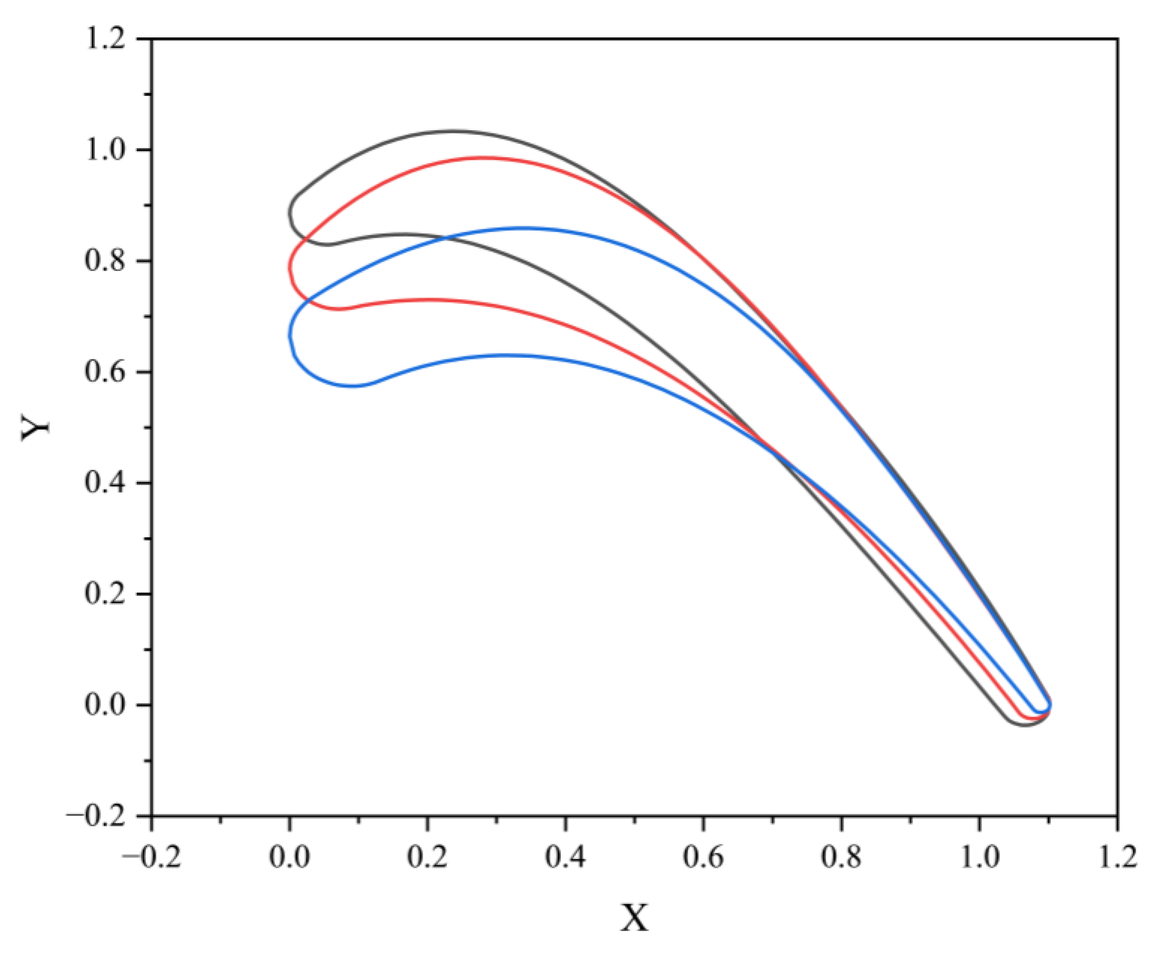
This study employs a Python 3.11-based implementation of Latin hypercube sampling (LHS) to ensure uniform distribution of samples in a multidimensional space. LHS is a widely used sampling method in high-dimensional design spaces, as it reduces the bias associated with traditional random sampling through uniformly distributed sample points, thereby improving the efficiency and accuracy of experiments. The parameter ranges used for LHS are based on publicly available engine blade profile data ranges, as shown in Table 1. Three blade profiles obtained via Latin hypercube sampling (with a sample size of 3) are presented in Figure 2. The sampling process strictly adheres to the parameter distribution range of the dataset, ensuring uniform coverage of the key design variable space. These representative blade profiles are generated under specific inlet and outlet geometric angles, which can fully reflect the diversity of geometric characteristics of all profiles in the dataset.

2.2. Mesh Generation and Flow Field Solution

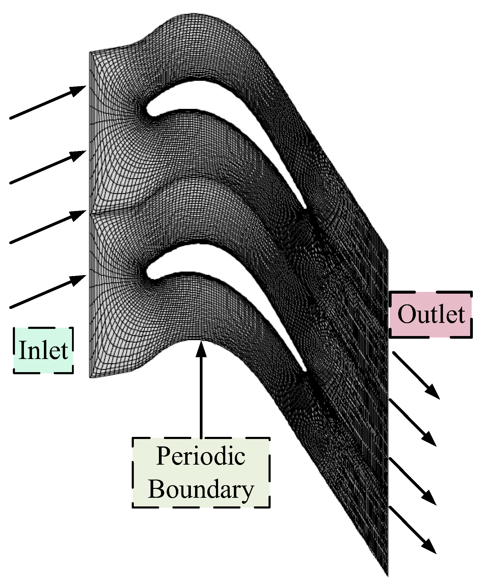
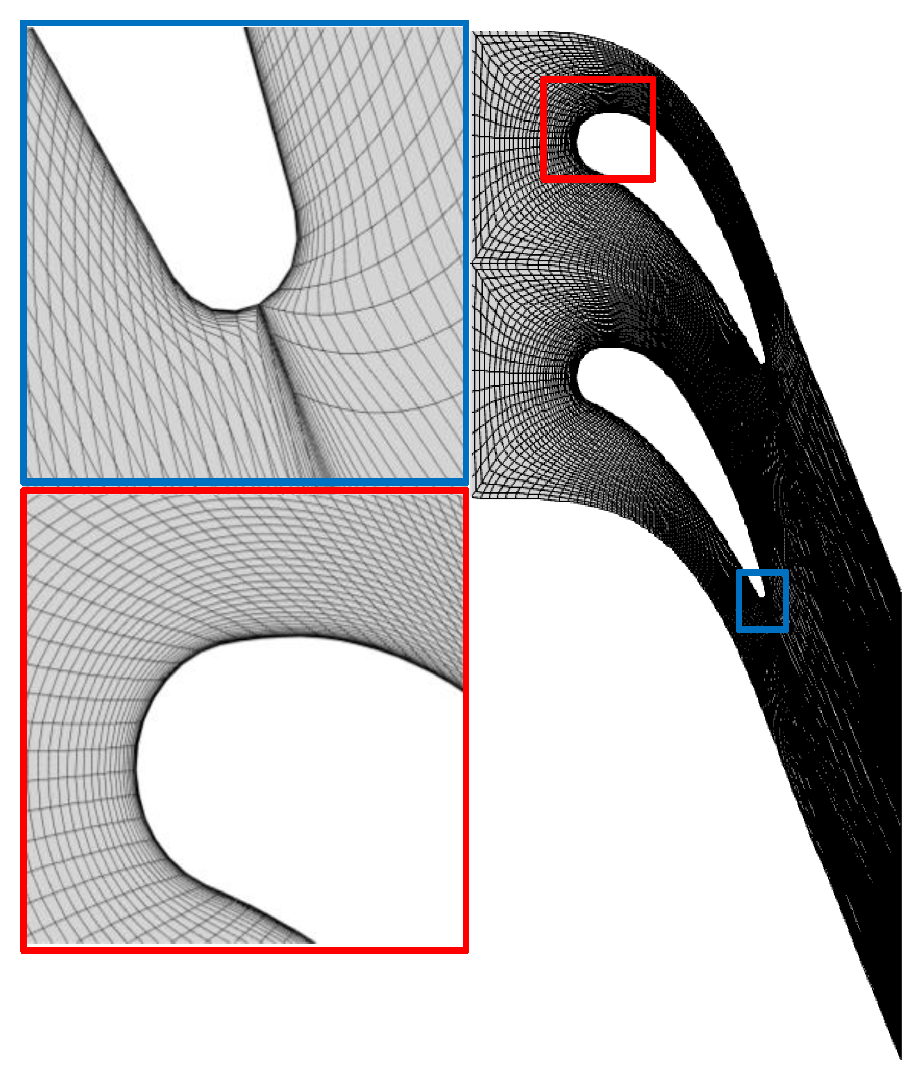
A two-dimensional C-type mesh generation program, developed by the author’s research group, was employed for mesh generation. The flow field was solved using the TQ3DNS program [32]. The input boundary conditions for the TQ3DNS program are shown in Table 2. This program uses the Baldwin–Lomax turbulence model [33]. The distance between the computational domain inlet and the blade inlet is 0.35 times the axial chord length. The distance from the computational domain to the blade outlet is 0.5 times the axial chord length, with the first layer y+ controlled at around 10. Figure 3 illustrates the computational mesh topology for a typical case within the geometric scope of the proposed 11-parameter blade profiling method. The blade profile depicted herein is not an aerodynamically optimized design but rather a representative example selected to demonstrate the mesh generation strategy, including element density distribution and boundary layer mesh refinement. The TQ3DNS program has been validated in previous studies [34,35,36].

2.3. Mesh Independence Verification and Computational Fluid Dynamics Program Validation

Prior to conducting the numerical simulations, a mesh independence verification was carried out to ensure that the computational accuracy of the TQ3DNS solver is not influenced by mesh density. The mesh sensitivity study was conducted based on the blade geometry illustrated in Figure 3, which shows the computational mesh topology for a typical cascade case generated within the geometric scope of the proposed 11-parameter blade profiling method. This representative airfoil was selected to reflect the characteristic features of the blade profiles investigated in the present study.
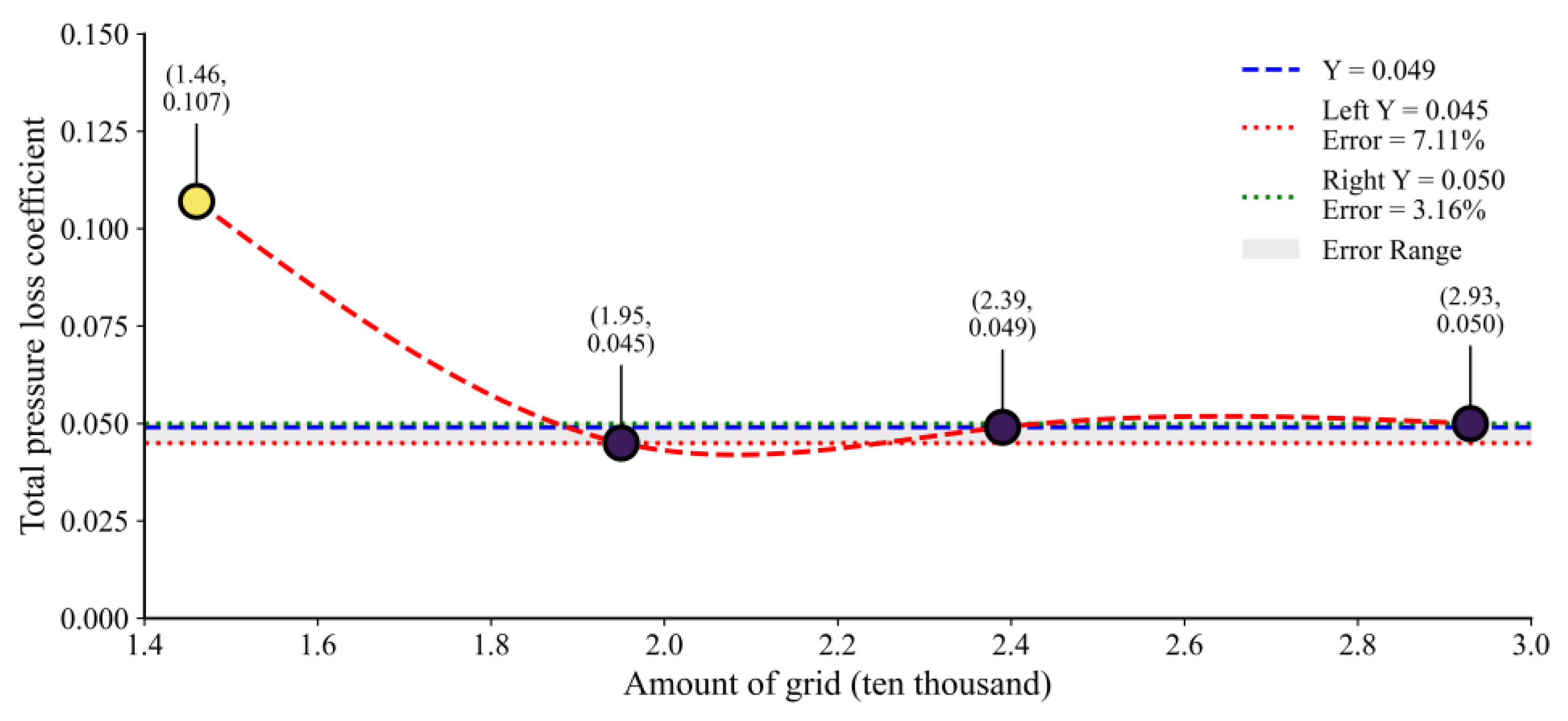
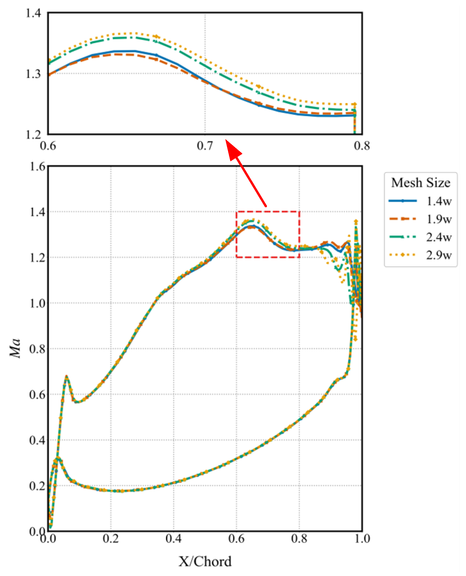
Figure 4 and Figure 5 present the calculated results obtained using different mesh quantities. Four mesh sets were tested, consisting of approximately 14,000, 19,000, 24,000, and 29,000 grid elements, respectively. The variation in the total pressure loss coefficient as well as the isentropic Mach number distribution along the blade surface was examined for each mesh configuration.
The results indicate that increasing the mesh density beyond 24,000 elements leads to only marginal changes in both global performance parameters and local flow characteristics. Therefore, the mesh with 24,000 elements was selected for all subsequent simulations, as it provides a satisfactory compromise between numerical accuracy and computational efficiency while meeting the requirements of the present study.
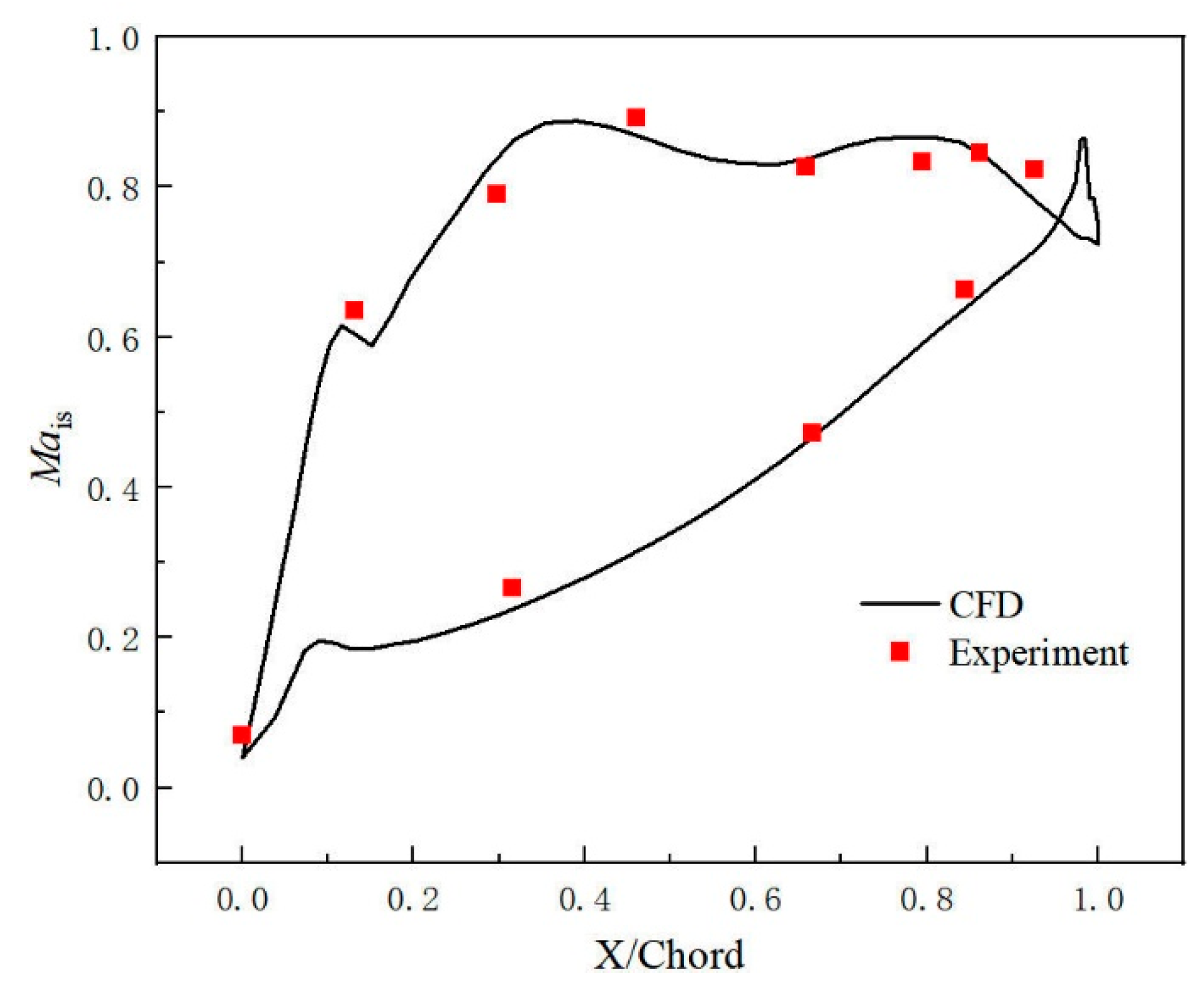
In the validation process of the CFD program, the Goldman cascade experiment is employed as a classic benchmark case and is widely used to verify the accuracy and reliability of CFD programs [37]. The data from this experiment are typically used to evaluate the reliability of CFD models in cascade flow simulation. The computational domain is defined such that the inlet boundary is 0.5 times the axial chord length from the cascade leading edge, while the outlet boundary is 1.0 times the axial chord length from the cascade trailing edge. The pitch is set at 41 mm. The total number of grid nodes in the entire computational domain is approximately 24,000, as shown in Figure 6. The boundary conditions are set as follows: the inlet boundary condition is a total temperature of 288 K, a total pressure of 101,325 Pa, and axial inflow; the outlet boundary condition is set to a static pressure of 69,914.25 Pa; the upper and lower boundaries adopt periodic boundary conditions. Flow parameters are based on the incoming flow conditions, using the chord length as the characteristic length, yielding a Reynolds number of 6.07 × 10⁶. Validation of the numerical method is performed by comparing the Mach number distribution obtained from CFD simulations with available experimental data for the Goldman cascade, as shown in Figure 7. Through comparative analysis, the deviation between CFD-calculated values and experimental data is within an acceptable range, indicating that the CFD program used can effectively predict the flow characteristics in the cascade region, verifying its reliability and accuracy in complex aerodynamic problems.

2.4. Dataset Construction and Splitting

The distribution of isentropic Mach number on the blade surface is represented as M a i s = x 1 , M a i s 1 , x 2 , M a i s 2 , , x 150 , M a i s 150 , the corresponding boundary conditions can be represented as b = b 1 , b 2 , b 3 , b 4 , b 5 , and the output blade coordinate points can be represented as g = x 1 , y 1 , x 2 , y 2 , , x 100 , y 100 . In summary, a database required for model training can be constructed with inputs comprising an input matrix formed by the blade surface isentropic Mach number and boundary conditions. Each data set includes 150 blade surface isentropic Mach number points and 5 boundary condition parameters. The output blade corresponds to blade coordinate points, with each data set containing 100 blade coordinate points. This study generated a total of 41,864 sample data sets. For training and validation, in terms of data division, 33,491 samples were randomly selected from the total sample data in the sample space as the training set, accounting for approximately 80% of the total data. Finally, the remaining 8373 samples serve as the test set, accounting for approximately 20% of the total data, used to evaluate the model’s generalization ability and performance in practical applications. Notably, this study directly outputs blade coordinate points instead of relying on design parameters from traditional parametric modeling methods. Parametric methods, limited by the preset forms of spline curve or Bezier curve control points, make it difficult to achieve a balance between local and global adjustments, and may lead to non-physical solution phenomena due to curvature discontinuity. In contrast, directly predicting discrete coordinate points avoids the modeling difficulties associated with complex mapping relationships between geometric parameters and aerodynamic performance, while inheriting the advantages of deep learning-based inverse design in terms of flexibility.

3. Theoretical Methods

3.1. Turbine Blade Optimization Framework Based on Sequence-to-Sequence Transformer Model

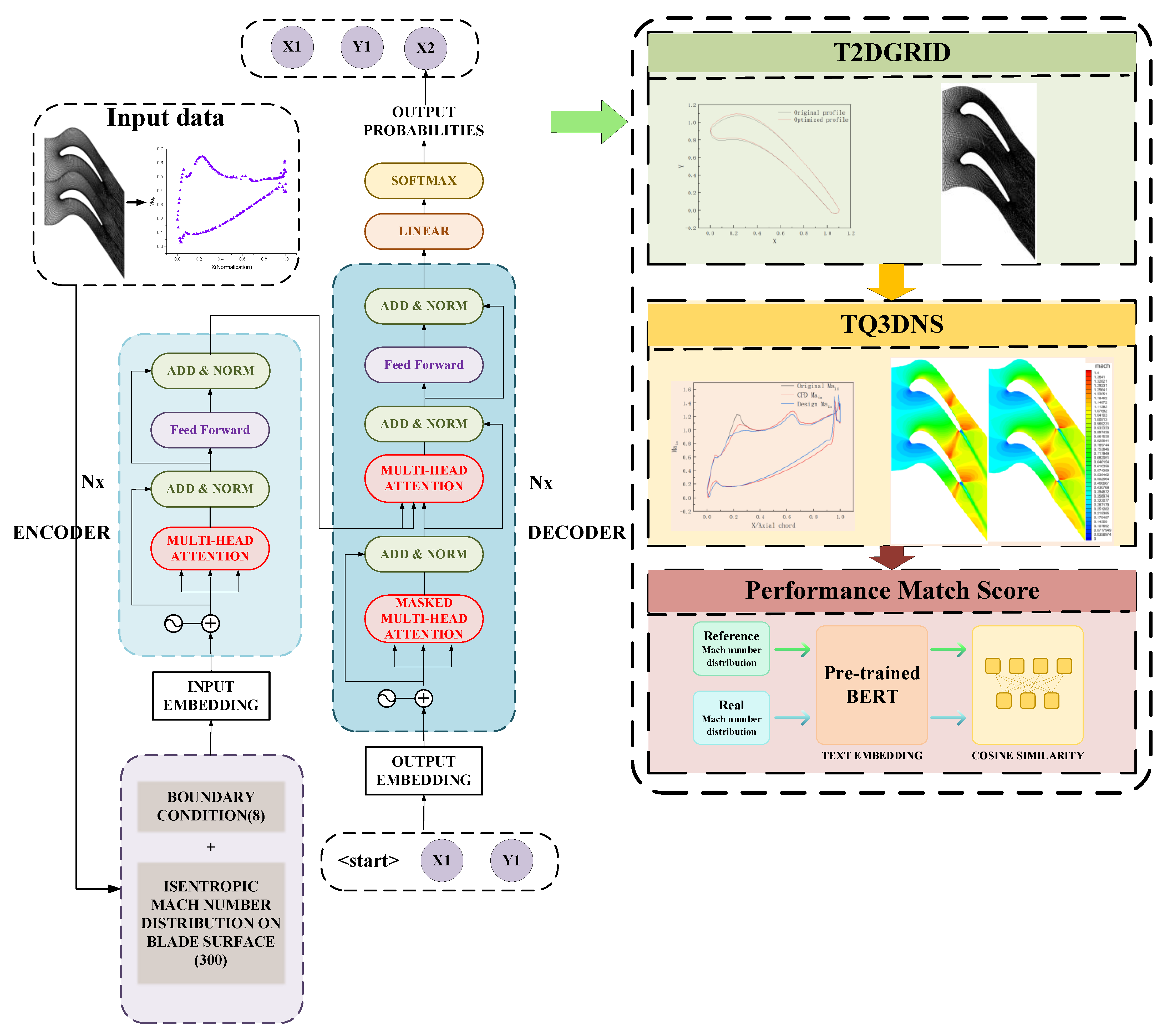
This study proposes a turbine blade design optimization method based on a sequence-to-sequence transformer model, as shown in Figure 8. This method addresses the core problems in traditional inverse problem design, such as low efficiency, convergence difficulties, and insufficient boundary condition accuracy, by establishing a direct mapping relationship between Mach number distribution and geometric coordinates. Unlike traditional methods that require iterative adjustment of geometric parameters or rely on physical model derivations, this method directly transforms the input Mach number distribution sequence into a blade coordinate sequence using a deep learning framework, avoiding technical bottlenecks such as mesh update difficulties in traditional virtual displacement methods and rough viscous treatment in transpiration boundary methods. The core idea of the transformer model is based on an encoder–decoder framework, capturing global dependencies in sequence data through a self-attention mechanism, which has significant advantages tackling aerodynamic–geometric coupling problems with complex nonlinear relationships. Compared to traditional optimization methods that require time-consuming processes combining CFD with repeated iterations, this method can produce blades that meet the target Mach number distribution without repeated iterations after training is completed, greatly improving design efficiency. The specific process is as follows:
First, designers select a known Mach number distribution as the initial input condition, modifying local distribution based on design requirements. The modified isentropic Mach number distribution and the corresponding boundary conditions are then input into the model. Embedding operations are used for the Mach number and boundary condition values at each position to obtain a continuous vector representation, preserving the semantic information of the original input. Position encoding methods are then used to add spatial information to each input, helping the model capture the spatial dependencies of parameters. The encoder captures the relationships between different input parameters (Mach number and boundary conditions). The decoder, leveraging a self-attention mechanism, gradually generates a blade coordinate sequence to address the limitations of traditional parameterization methods regarding geometric degrees of freedom. The blade coordinate points output by the model are used to generate a mesh through T2DGRID. Combined with the boundary conditions in the input, the actual Mach number distribution curve is obtained through CFD calculations. Both the actual and designed Mach number distribution curves are vectorized and mapped to high-dimensional vectors. The cosine similarity between each row is calculated to measure the generalization ability and adaptability of the constructed method.
The transformer model was selected over traditional MLP or CNN owing to its superior ability to explicitly capture global information. While MLP and CNN are typically only effective for processing local information, easily overlooking global factors such as curvature changes and complex boundary condition interactions. These limitations can lead to issues such as poor generalization ability and curvature discontinuity in the prediction of curve coordinate points. In contrast, the transformer model can effectively capture global dependencies through the self-attention mechanism, thereby overcoming the difficulties of these localized models. The key challenges addressed in this study primarily include capturing the correlation among isentropic Mach number distributions along the blade surface, correlation between isentropic Mach number distribution along the blade surface and blade coordinates, and correlation among blade coordinates themselves.
Furthermore, the transformer model was also selected because it can process blade coordinate points as “tokens,” which is different from traditional regression problems. By viewing coordinate points as elements (tokens) in a “language,” the transformer model can leverage the ideas of language models to capture sequence patterns and contextual relationships between coordinate points. This approach can incorporate more structured information into predictions, enhancing the model’s generalization ability and avoiding discontinuity problems in regression methods. This approach shifts from predicting the specific values of each X or Y in a regression problem to “connecting” points from the set of all points in the test set to form a new blade profile. Although this processing may result in poor performance of the new blade profile when sample points are limited, the adoption of the transformer model necessitates a large dataset.
During model training and application, some issues persist, needing further discussion. First, establishing a direct connection between the adjusted Mach number distribution and the model-predicted coordinates is difficult. Second, the prediction accuracy of the model is not equivalent to its generalization ability. High prediction accuracy may be owing to the fact that all blade profiles are generated through the 11-parameter modeling method, resulting in similar probability distributions in the training, validation, and test sets. However, in practical applications, when designers adjust the Mach number probability distribution, the new distribution may differ significantly from the training data, thereby affecting the model’s generalization ability. Therefore, ensuring robust generalization ability across different design scenarios remains a key challenge for the current model. To address this, this study proposes a quantitative evaluation metric based on Mach number distribution similarity. Specifically, the actual Mach number distribution curve can be obtained by predicting the blade profile and performing CFD calculations. Subsequently, the actual and theoretical Mach number distribution in the design can be vectorized and mapped to high-dimensional vectors. Then, the cosine similarity between the two vectors is calculated to measure their degree of difference, thereby quantitatively evaluating the model’s generalization ability and adjustment effect. Moreover, by introducing this quantitative metric, the optimization direction of the model can be further explored, and a reliable feedback mechanism can be provided for Mach number adjustments in the actual design.

3.2. Transformer Principles

The primary structure of the transformer model includes two major parts: encoder and decoder, each comprising multiple identical layers stacked together. Each layer contains a self-attention mechanism and a feedforward neural network (FFNN), with position encoding compensating for the lack of sequence information. The following subsections will elaborate on the four key components of the transformer model and their roles.

3.2.1. Attention Mechanism

The self-attention mechanism in the transformer model calculates the weighted representation of each position through three vectors: query (Q), key (K), and value (V). Assuming the input sequence is X, the representation at each position can be calculated using the following formula:
A t t e n t i o n Q , K , V = s o f t m a x Q K T d k V
where Q is the query vector, K is the key vector, V is the value vector, and dk is the dimension of the key vector. This operation calculates the similarity between queries and keys through dot products, thereby obtaining a weight matrix, which is then multiplied with the value vector to generate the final output.

3.2.2. Position Encoding

Position encoding in the transformer model typically uses sine and cosine functions to ensure that encodings in different dimensions have different periodicities. The formula for position encoding is provided below:
P E p o s , 2 i = s i n p o s 10000 2 i / d
where pos denotes the position, i is the dimension index, and d is the dimension of the positional encoding. This design allows the model to capture the relative positions of elements in the sequence by combining encodings across different dimensions.

3.2.3. Feedforward Neural Network

Each transformer layer includes a FFNN in addition to the self-attention mechanism. The FFNN module typically comprises two fully connected layers with a nonlinear activation function. Specifically, the FFNN in the transformer model is structured as follows:
F F N N x = m a x 0 , x W 1 + b 1 W 2 + b 2
where W1 and W2 are weight matrices, b1 and b2 are bias terms, and the activation function is usually ReLU or another nonlinear function.

3.2.4. KL Divergence Loss Function

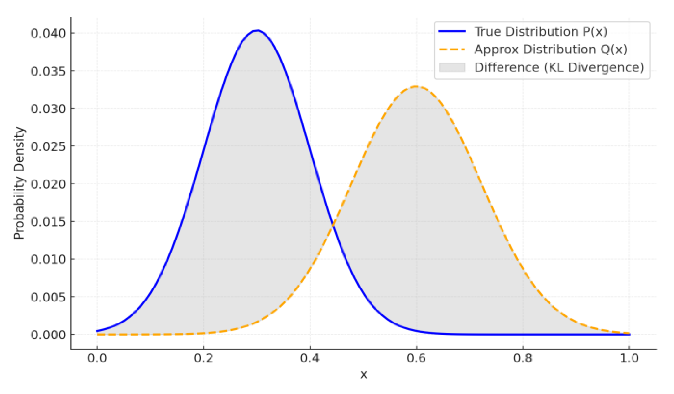
The Kullback–Leibler (KL) divergence loss measures the difference between two probability distributions (Figure 9). In the context of sequence generation tasks such as the inverse design of blade profiles, the KL divergence is particularly suitable for guiding the model to produce geometric sequences that align with the true data distribution. Unlike traditional regression loss functions such as Mean Squared Error (MSE) or Mean Absolute Error (MAE), which focus solely on pointwise differences between predicted and target coordinates, the KL divergence evaluates the discrepancy in the overall probability distribution of the generated sequences. This characteristic is crucial in aerodynamic design, where the global shape consistency and smoothness of the blade profile often matter more than the exact match of individual coordinate points.
Specifically, in this study, the blade coordinate prediction is treated as a conditional sequence generation problem. The KL divergence helps the model learn not only the local geometric features but also the global structural dependencies inherent in blade profiles. By minimizing the KL divergence between the predicted and target coordinate distributions, the model is encouraged to generate profiles that are not only accurate in a pointwise sense but also physically plausible and aerodynamically consistent.
The KL divergence is defined as follows:
D K L P Q = x P x l o g P x Q x
where P is the target distribution and Q is the model’s predicted distribution. By minimizing the KL divergence during training, the model’s predicted distribution gradually aligns with the true data distribution, thereby improving the quality and physical realism of the generated blade profiles.

3.3. Performance Matching Metric

In turbine blade design, establishing a direct mapping between the adjusted Mach number distribution and the coordinates predicted by the model is inherently challenging. This is because modifications to the Mach number distribution changes the geometric characteristics of the blade, making true coordinates of the new blade uncertain. Moreover, improved prediction accuracy of the model does not necessarily imply strong generalization ability. High accuracy may simply reflect similarities across the training, validation, and test sets, and the model performs well on these datasets. However, when faced with new design adjustments, the model’s performance may decline. The use of an 11-parameter modeling method used in the blade generation process ensures high consistency between training and test data distributions, yet in practical applications, designers may adjust the Mach number distribution, potentially affecting the model’s predictive ability because of differences in the training data. Neural network models, while powerful, are not universally robust; they may perform prediction tasks well under certain conditions but fail under others. Therefore, there is an urgent need for a performance matching metric to help designers in assessing the reliability of model predictions for new design tasks.
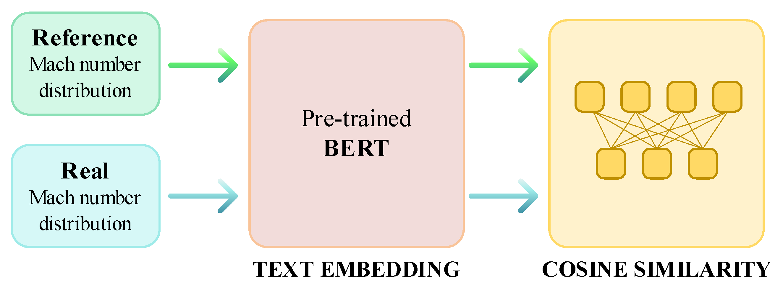
To overcome this limitation, this study proposes a quantitative metric based on Mach number distribution similarity as a criterion for model performance evaluation. By mapping the predicted distributions and theoretical distributions into high-dimensional vectors and calculating their cosine similarity, the metric quantitatively evaluates the model’s generalization ability and adjustment effect, as shown in Figure 10.
Specifically, this method operates according to the following steps: In turbine blade design, we first obtain the Mach number distribution M p r e d x of the model-predicted blade through CFD calculations, where x represents the parametric position on the blade surface, and compare it with the theoretically designed Mach number distribution M t r u e x . To effectively process these distributions and capture their complex structures, we use the BERT embedding model to vectorize the Mach number distributions:
v p r e d = E m b e d M p r e d x
v t r u e = E m b e d M t r u e x
where Embed represents the BERT embedding process, capturing global dependencies in the input data through the self-attention mechanism, which is particularly suitable for data with spatial and non-linear characteristics such as Mach number distributions. BERT can effectively model the contextual relationships between Mach number points, reducing the impact of local errors.
After vectorization, cosine similarity is used to quantify the similarity between the predicted and theoretical distributions:
C o s i n e S i m ν p r e d , ν t r u e = ν p r e d ν t r u e ν p r e d ν t r u e
where the dot product ν p r e d ν t r u e measures the similarity between vectors, and the normalization terms ν p r e d and ν t r u e ensure the consistency of the similarity scale. The closer the cosine similarity is to 1, the more similar the predicted and designed Mach number distributions are.

4. Transformer Model Design

In this research, a sequence-to-sequence model based on the transformer architecture was designed and implemented to solve the inverse design optimization problem of blade profiles. As shown in Table 3, the model’s encoder and decoder comprise 5 stacked Encoder and Decoder layers, each containing multi-head attention mechanisms, feedforward networks, residual connections, and normalization processing. This design fully leverages the high-dimensional representation modeling capability of the transformer model, especially the advantages of the self-attention mechanism in capturing complex nonlinear relationships and global dependencies. The input and target sequences are first processed through embedding layers and positional encoding before being fed into the transformer model. The model parameters include 512 encoder–decoder hidden nodes, 2048 feedforward layer hidden nodes, 8 heads for multi-head attention, and a dropout rate of 0.1 during training. To accelerate model convergence and enhance robustness, the Noam learning rate scheduling strategy is adopted, and label smoothing technique is introduced to reduce the risk of overfitting.

5. Analysis of Blade Profile Optimization Results

5.1. Evaluation of CNN-CBAM Model Prediction Performance

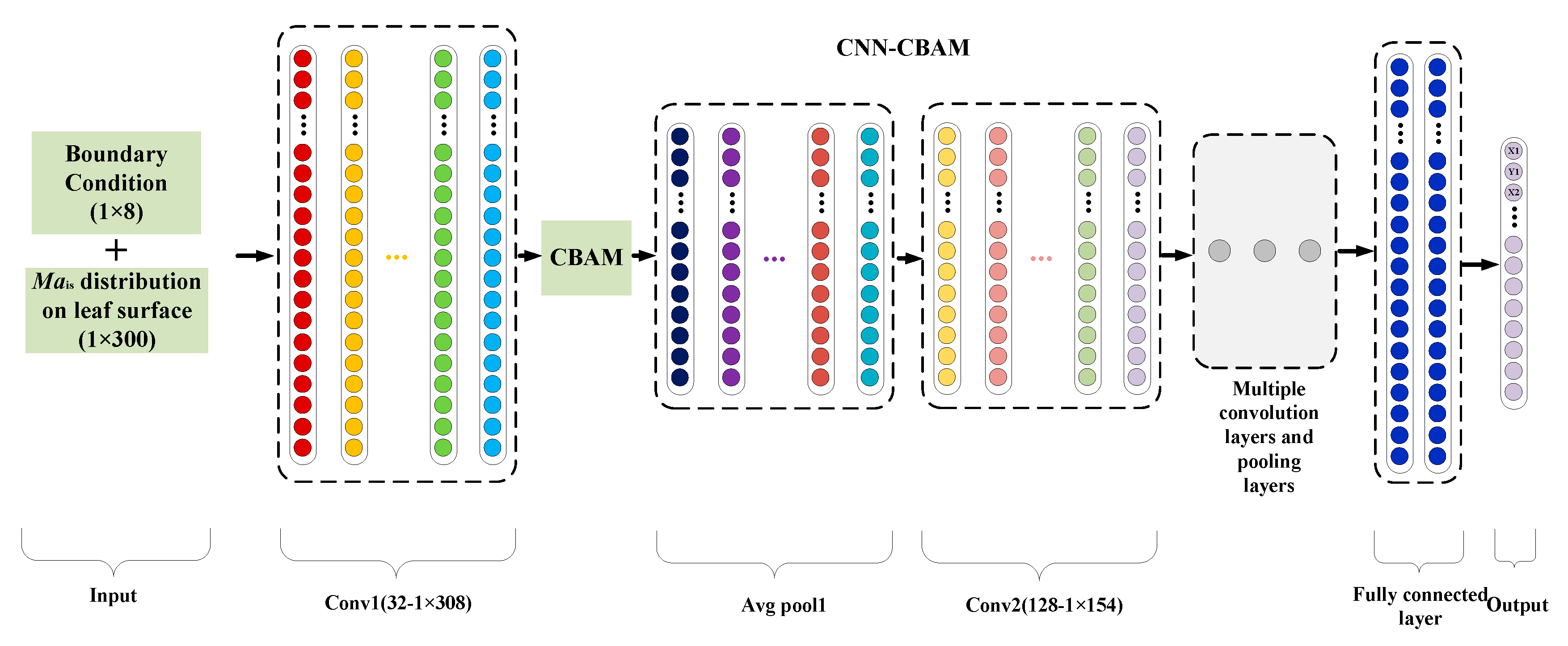
To enable a comparative analysis with the subsequent transformer-based method, this study first employs a Convolutional Neural Network with Convolutional Block Attention Module (CNN-CBAM) for the inverse design prediction of blade profiles. The CBAM mechanism enhances a traditional CNN by sequentially applying channel attention and spatial attention, enabling the model to adaptively focus on critical regions of the input features.
Specifically, the channel attention module identifies ‘what’ is important by emphasizing feature maps that are most informative for the coordinate prediction task. Subsequently, the spatial attention module determines ‘where’ to focus by highlighting salient spatial locations within those emphasized feature maps. In the context of blade profile inverse design, this synergistic mechanism theoretically guides the model to prioritize features associated with geometrically sensitive areas, such as the high-curvature leading edge and the suction surface, where precise shape control is crucial for aerodynamic performance. By amplifying features from these key regions, the CNN-CBAM model aims to achieve more accurate local geometric predictions than a standard CNN. The overall model structure is shown in Figure 11 and mainly includes several convolutional layers, pooling layers, CBAM modules, and fully connected layers. The overall structural parameters are detailed in Table 4.
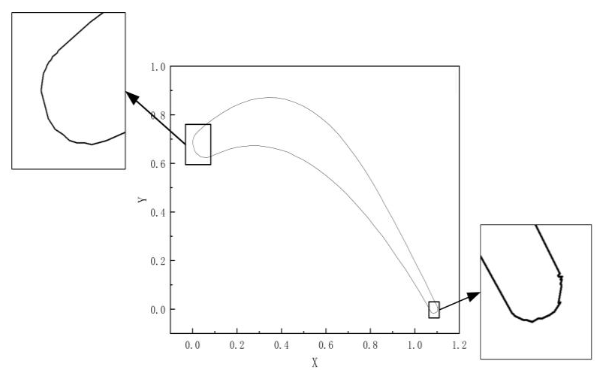
When testing a specific blade profile, the isentropic Mach number distribution on the blade surface is manually adjusted, and modified Mach number and boundary conditions are input into the model. The resulting optimized blade profile is shown in Figure 12. The results indicate that the CBAM mechanism still fails to fully guarantee smooth curvature continuity at key positions such as the leading and trailing edges. Excessive local curvature changes may lead to flow separation and Mach number fluctuations, affecting overall performance. Therefore, although CNN-CBAM model demonstrates certain effects in addressing the inverse design problem of blade profiles and curvature discontinuity, there remains significant potential for further optimization.

5.2. Evaluation of Transformer Model Prediction Performance

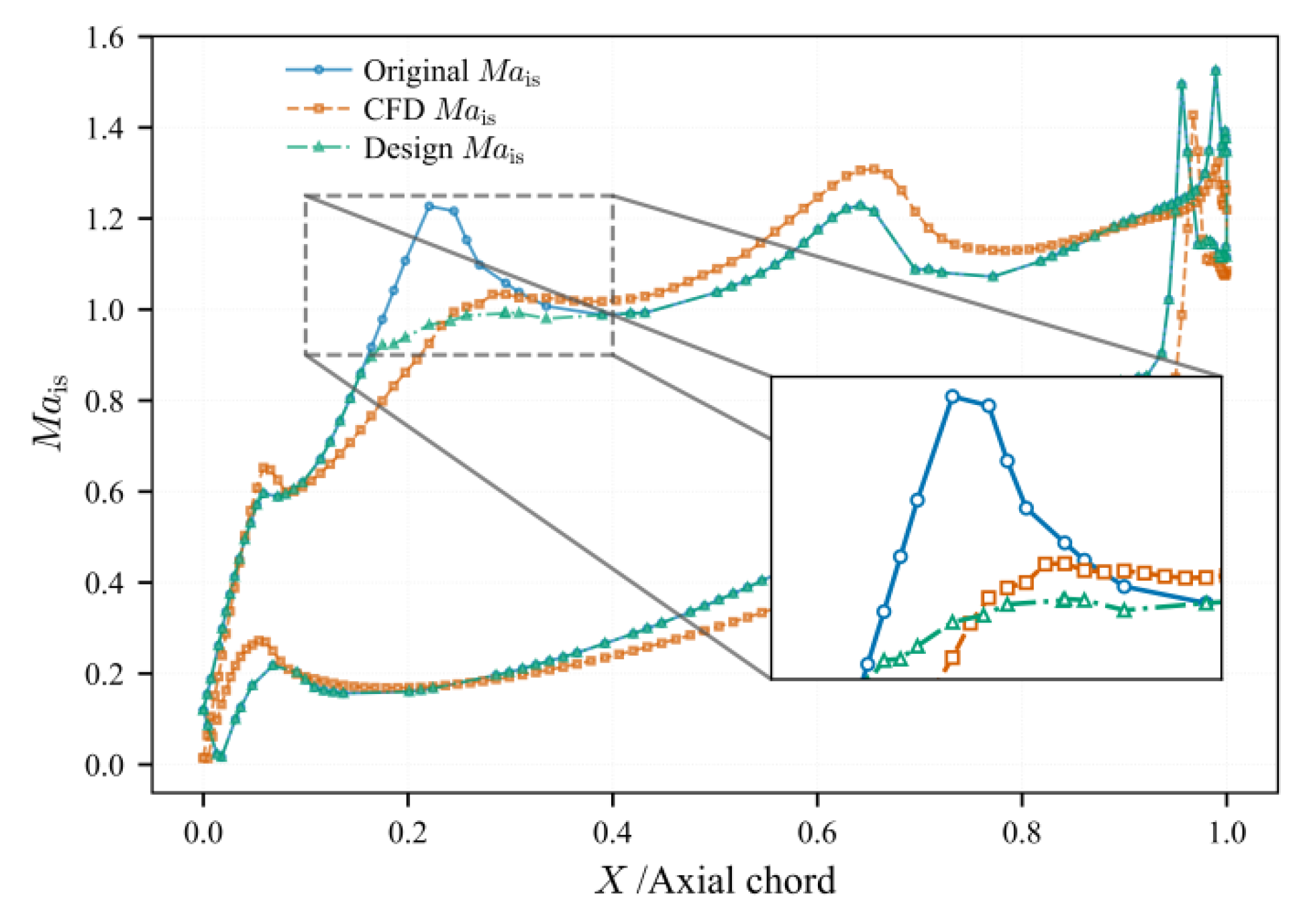
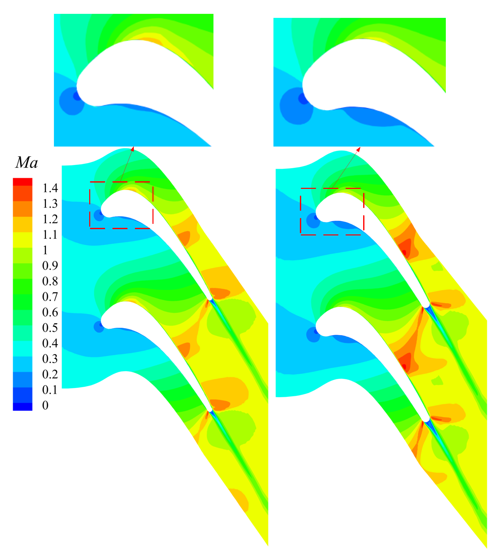
During specific operations, designers can screen out initial Mach number distribution schemes that meet load distribution requirements from the dataset and then complete the final design requirements by optimizing the isentropic Mach number distribution. To verify the effectiveness of the method, this study takes a certain turbine blade profile as an example and conducts optimization verification by fine-tuning its Mach number distribution. Figure 13 shows the original blade profile’s Mach number distribution, the expected Mach number distribution designed manually, and the Mach number distribution corresponding to the blade profile predicted by the model. Figure 14 compares the Mach number contours between the original blade profile and the optimized blade profile.
Unlike global reshaping of the Mach number distribution, the optimization mainly targets the suction-side leading-edge acceleration region. As shown in Figure 13, the optimized blade exhibits a reduced Mach number peak on the suction surface near the leading edge, leading to a more moderate Mach number variation within the axial chord range of X/Axial chord ≈ 0.17–0.30.
This reduction in the suction-side leading-edge Mach number peak alleviates excessive local acceleration and results in a relatively smoother Mach number gradient in the front portion of the blade. Such behavior is desirable, as it helps suppress sharp acceleration-induced losses and improves flow stability in the leading-edge region.
In this axial range, the CFD-predicted Mach number distribution of the optimized blade closely approaches the target design distribution, indicating that the airflow acceleration behavior on the suction surface has been effectively improved and brought closer to the intended aerodynamic design state.
These results demonstrate that the transformer-based model is capable of accurately capturing and implementing designer-specified Mach number distributions. By prescribing the target Mach number distribution as input, the model can generate a corresponding blade geometry whose CFD results exhibit close agreement with the desired distribution. This confirms that the proposed approach has strong practical applicability and prediction accuracy for turbine blade optimization.
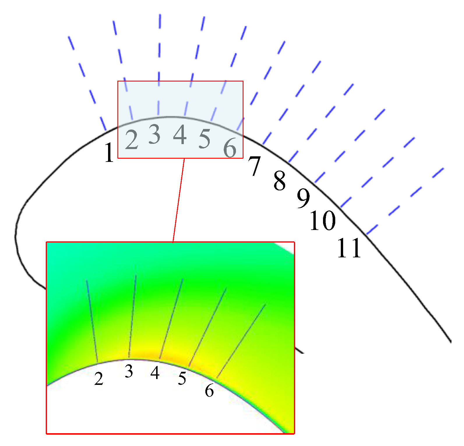
Velocity distributions at 11 locations along the blade surface are extracted, as shown in Figure 15. These distributions are used to further evaluate the effectiveness of the proposed turbine blade design optimization framework based on the sequence-to-sequence transformer model. The selected locations cover key regions of interest, including the modified position, areas before and after the modified position, and other areas of the blade surface.
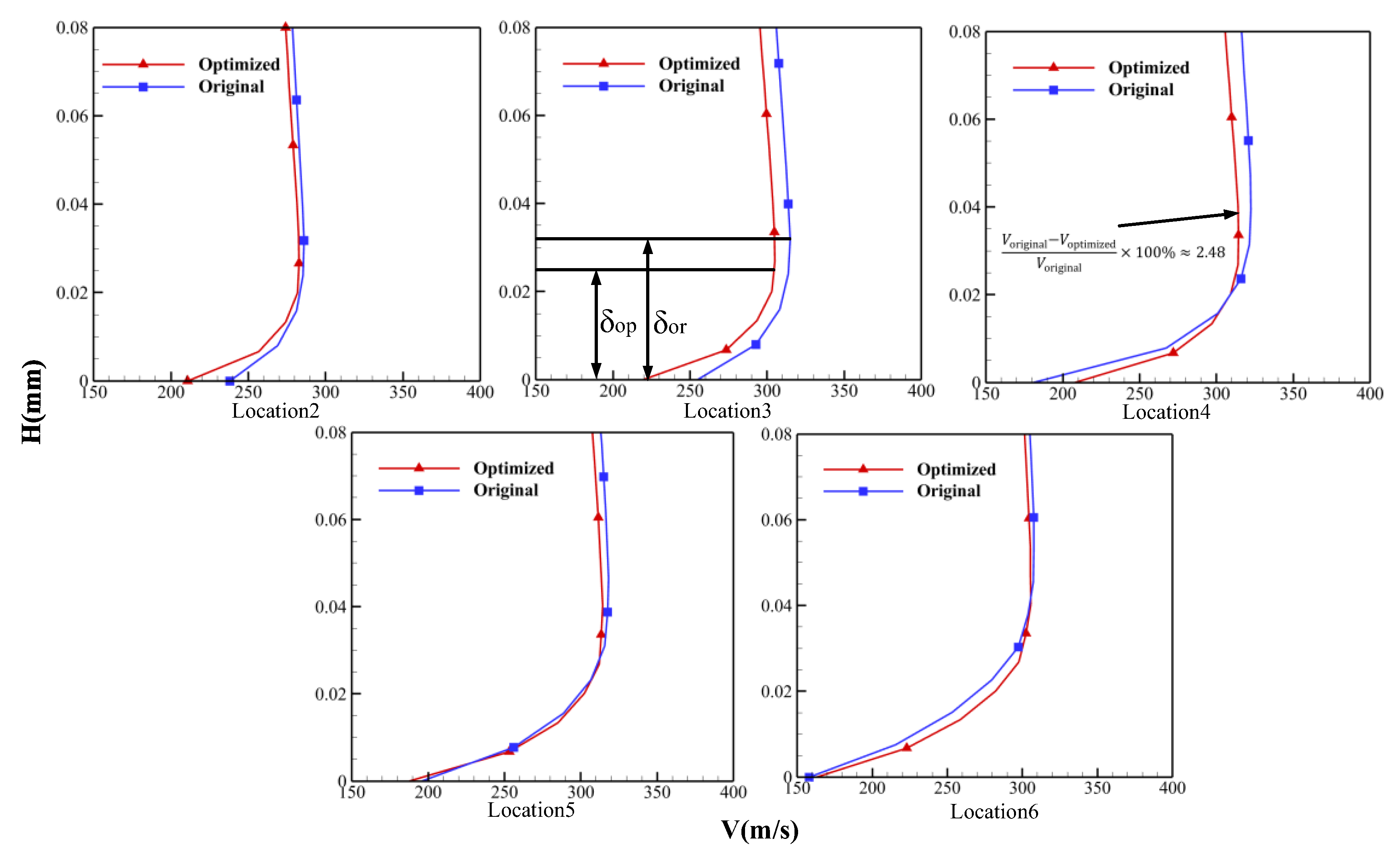
Figure 16 shows the velocity distribution profiles on each curve. It can clearly be seen that the leading-edge acceleration zone is mainly concentrated at positions 3, 4, and 5, which is consistent with the local details shown in Figure 15. The maximum near-wall velocities at position 4 for the original and optimized cascades are 322 m/s and 314 m/s, respectively, with the optimized cascade showing a 2.48% velocity reduction, which is in line with the design optimization expectations. Before the acceleration zone, there is little difference in the velocity distribution and boundary layer thickness near the wall between the original and optimized blade profiles, indicating that the optimization of the blade profile has not changed the adaptability to inlet flow. Within the acceleration zone, the velocity distributions of the two blade profiles begin to show significant differences; however, these differences gradually disappear after the acceleration zone, and the two blade profiles each develop into the same form of velocity distribution. Comparatively, the optimized cascade has a thinner boundary layer thickness after the acceleration zone, which improves the total pressure recovery coefficient of the turbine. The total pressure recovery coefficients of the original and optimized profiles are 0.949 and 0.954, respectively. Furthermore, the total pressure loss coefficient, a key metric for turbine efficiency, decreases from 0.744 (original design) to 0.663 (optimized design), confirming the aerodynamic improvements from the optimization. In summary, local optimization of turbine blades based on the transformer method is feasible, and the local optimization does not change the main flow structure at other positions. Additionally, the improvement of flow in the leading-edge acceleration zone has a significant impact on reducing turbine losses.
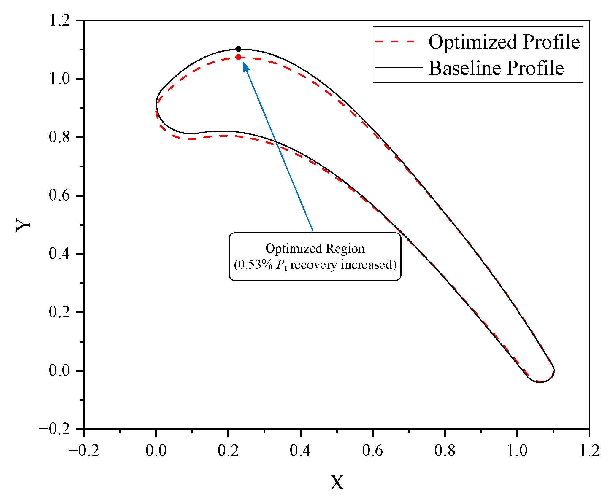
Figure 17 compares the optimized blade profile and the original blade profile. When comparing the geometric characteristics of the original and optimized blade profiles and their impact on aerodynamic performance, it can be seen that the optimized blade profile has a gentler curvature change near X = 0.2. These geometric characteristics make the pressure gradient in this region of the optimized blade profile more uniform, weakening the local sudden acceleration area and smoothening the flow acceleration process smoother. In contrast, the original blade profile has larger curvature changes in the same region, leading to uneven pressure gradients and sudden flow acceleration, which affect its aerodynamic performance.
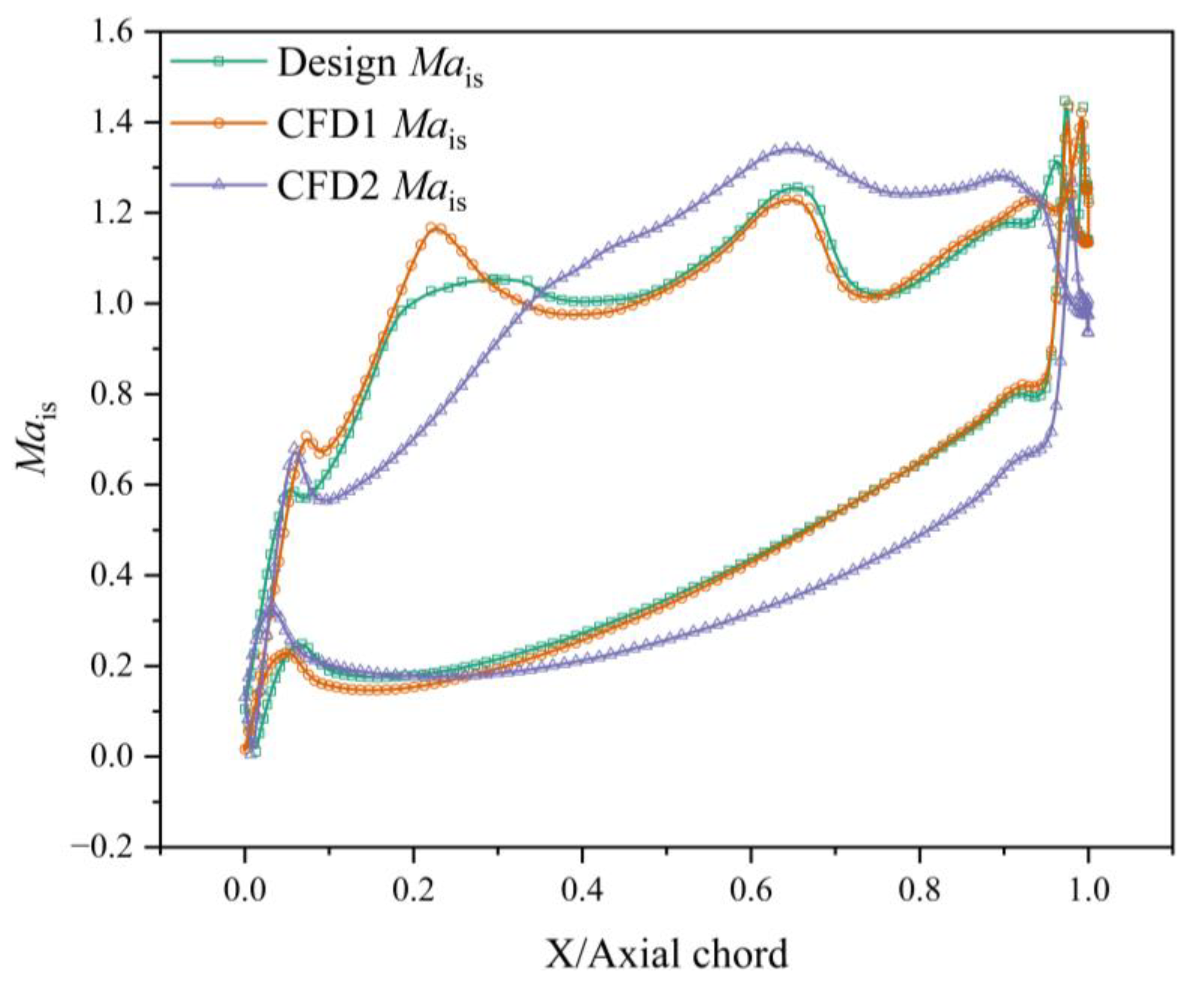
Figure 18 and Figure 19 provide a detailed evaluation of the model’s performance by comparing two blade profiles generated using different internal parameter sets of the transformer model. Figure 18 presents a direct comparison between the CFD-computed isentropic Mach number distributions of the two predicted blade profiles and the designer-specified target distribution. The CFD1 profile (red curve) exhibits closer agreement with the target Mach number distribution over most of the blade surface, particularly along the suction surface, which is critical for aerodynamic performance. In contrast, the CFD2 profile (blue curve) shows noticeable deviations from the target distribution. This comparison highlights that, although the same target Mach number distribution and boundary conditions are used, the predictive quality of the inverse design results can vary depending on the model parameters, thereby motivating the need for a quantitative evaluation metric.
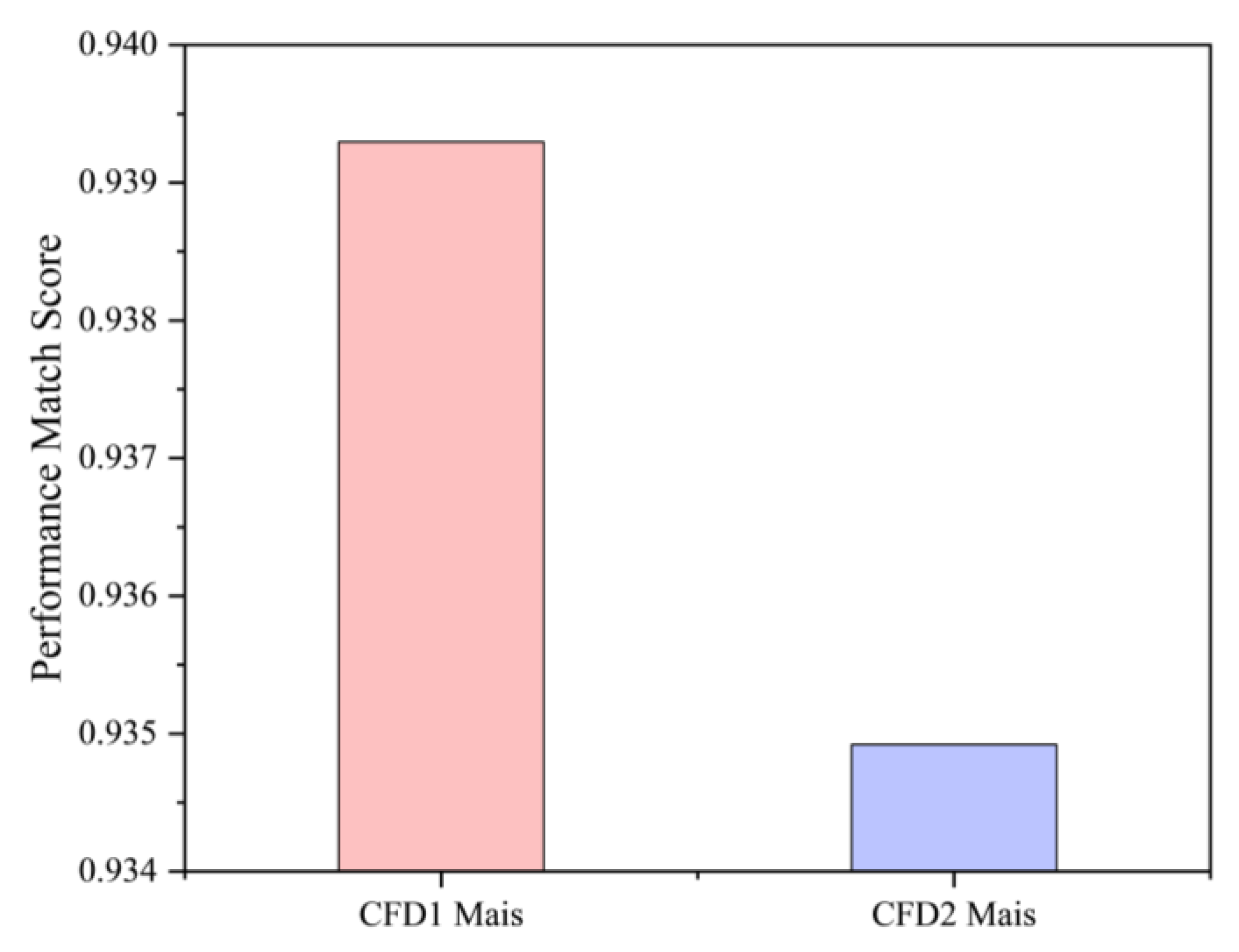
The Performance Match Score shown in Figure 19 is introduced to serve as this quantitative evaluation criterion. It measures the degree of similarity between the CFD-computed Mach number distribution of a predicted blade and the designer-prescribed target distribution. As illustrated by the bar chart, the Performance Match Score of the CFD1 profile is significantly higher than that of the CFD2 profile, which is fully consistent with the qualitative trends observed in Figure 18. This metric is particularly important because the true blade geometry that exactly satisfies the designer’s intent is generally unknown in inverse design problems. Consequently, the Performance Match Score is used to indicate how closely a predicted blade profile approaches this unknown, ideal solution. A low score suggests poor agreement with the target performance and may indicate that the inverse problem is ill-posed or lacks a viable solution under the given model configuration. By providing a quantitative and objective measure of performance alignment, this metric offers valuable feedback for model selection and enhances the reliability of the proposed AI-driven turbine blade design framework.
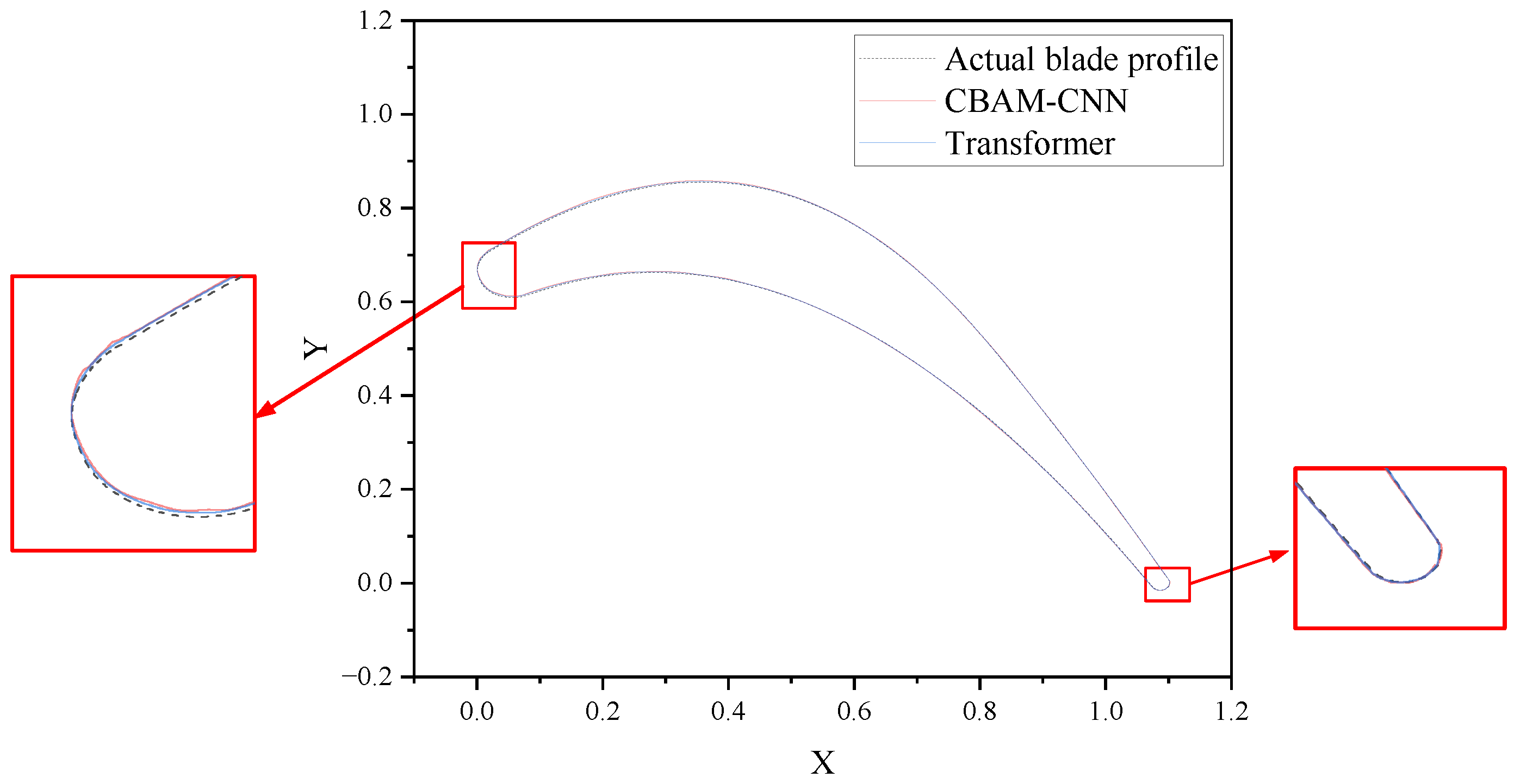
Figure 20 presents a comparison of blade profile geometries from the test set, including the ground truth profile (gray line), the CBAM-CNN model prediction (red line), and the Transformer model prediction (blue line).
The CBAM-CNN prediction exhibits strong geometric discontinuities, particularly in the leading-edge and trailing-edge regions. These discontinuities appear as abrupt changes in curvature, which are aerodynamically unacceptable for turbine blade design. Such behavior is primarily attributed to the intrinsic characteristics of CNN-based architectures, which rely on local convolutional kernels and spatial pooling operations. While effective for extracting local features, CNNs lack an explicit mechanism to capture global, long-range geometric dependencies, making it difficult to enforce smoothness and curvature continuity along the entire blade surface.
In contrast, the sequence-to-sequence Transformer model produces a blade profile with smooth and continuous curvature transitions from the leading edge to the trailing edge. By treating blade coordinate points as ordered tokens in a sequence, the Transformer leverages a self-attention mechanism to model global interactions among all points simultaneously, thereby preserving geometric coherence and suppressing non-physical discontinuities. The Transformer’s ability to capture long-range dependencies and global shape characteristics makes it inherently more suitable for inverse aerodynamic design tasks, where geometric smoothness and physical feasibility are essential.
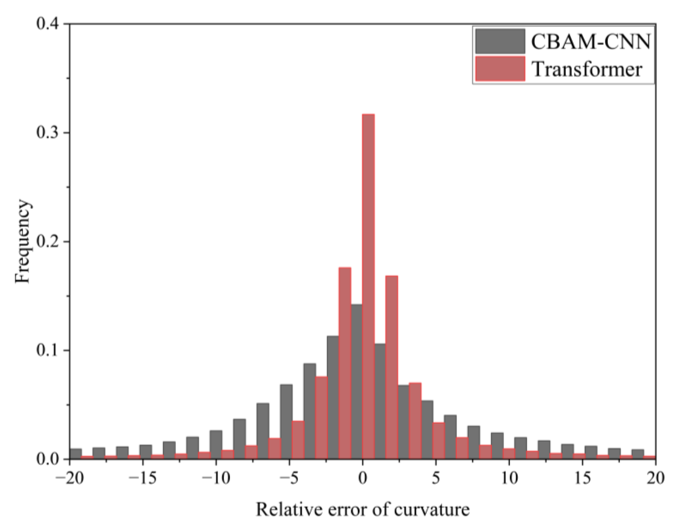
Figure 21 displays the histogram of curvature error distributions for the CBAM-CNN model (dark gray bars) and Transformer model (red bars) across the test set. Traditional turbine optimization methods typically predict a limited number of design parameters (e.g., airfoil parameterization coefficients or Bézier curve control points), which inherently constrain geometric freedom. In contrast, our proposed approach directly predicts coordinate points, offering a more flexible and high-dimensional design space. However, this increased freedom poses a challenge for traditional neural network architectures: predicting a large number of coordinate points makes it difficult to ensure curvature continuity, as these models lack mechanisms to model sequential dependencies between points. Inspired by natural language processing, our Transformer model leverages a sequence-to-sequence framework and self-attention mechanism to learn the positional relationships of previously generated coordinate points, enabling it to predict the next point while maintaining smooth curvature transitions. The curvature relative error distribution of the CBAM-CNN model is relatively scattered, with notable frequency distributions in the error ranges of −15 to −5 and 5 to 15. In contrast, the curvature relative errors of the Transformer model are primarily concentrated within the small error range of −5 to 5, with a peak frequency of about 0.325, and the frequency in large error ranges beyond ±10 is nearly zero. The results indicate that the curvature prediction error of the Transformer model is smaller than that of the CBAM-CNN model, demonstrating its superior accuracy in predicting blade profile curvature.

5.3. Model Prediction Accuracy and Error Statistical Analysis

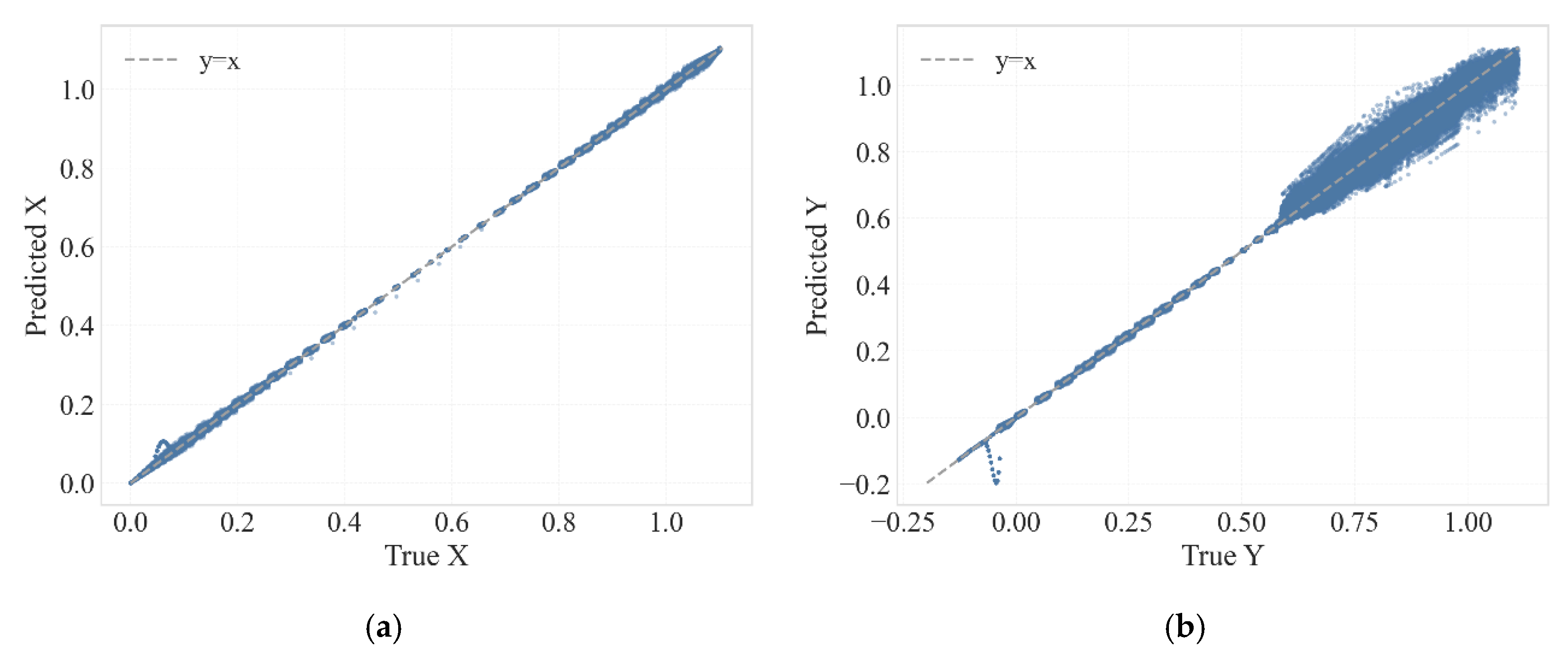
To comprehensively verify its reliability in the blade coordinate prediction task, the prediction accuracy, consistency, and error distribution of the Transformer model were quantitatively evaluated using various statistical methods. Figure 22 shows a scatter plot comparing the predicted values against the true values for the entire test set. As shown in the figure, for both the X and Y coordinates, most of the scatter points lie close to the ideal diagonal line (y = x). The high correlation indicates that the Sequence-to-Sequence Transformer model constructed in this study has successfully learned the complex and precise mapping relationship between aerodynamic parameters and geometric coordinates, demonstrating high prediction accuracy and reliability.
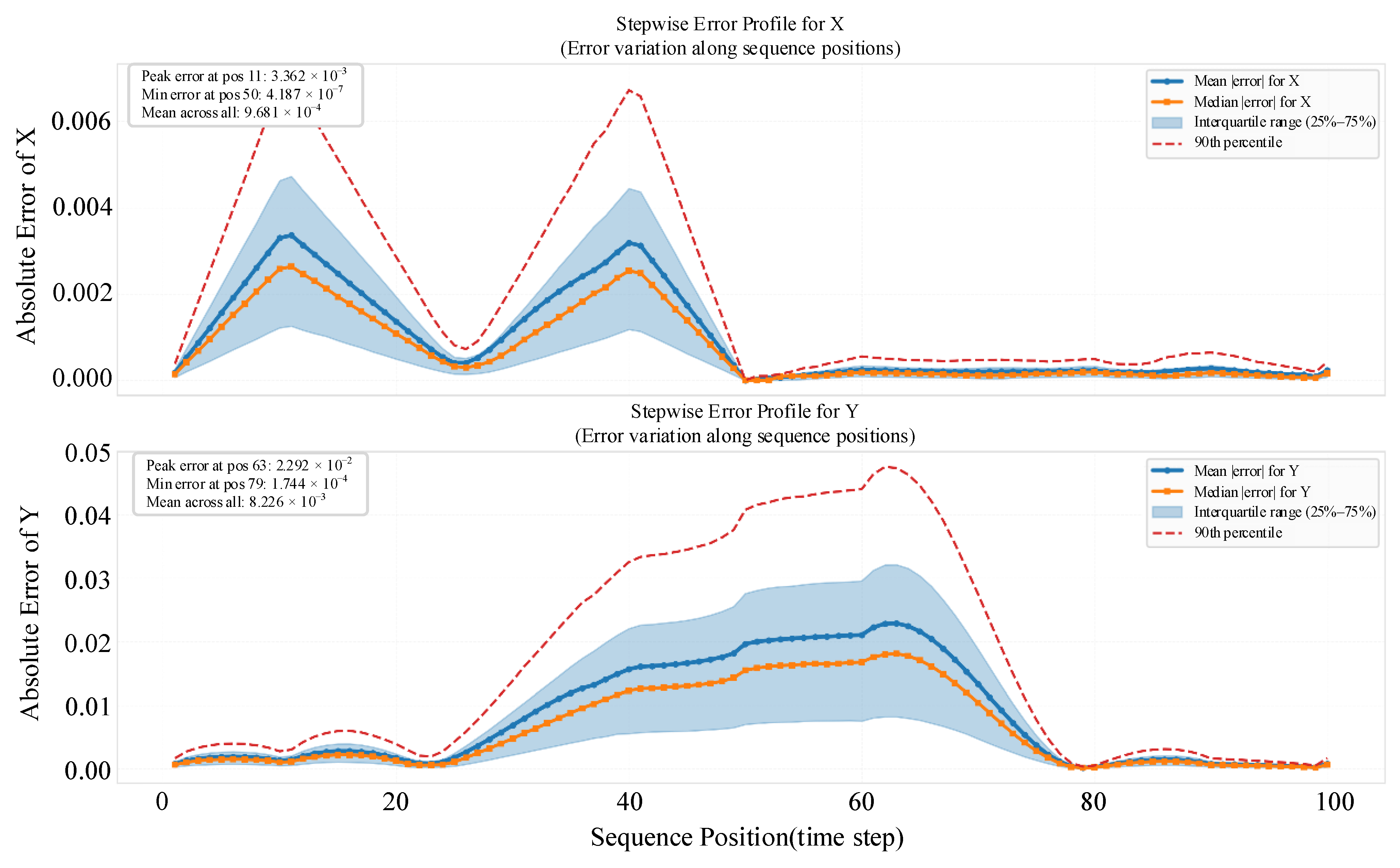
Figure 23 reveals the distribution of prediction errors along different positions (sequence positions) on the blade surface, which is crucial for identifying the model’s weaknesses and guiding optimization design. Analysis shows that the prediction error for the X-coordinate peaks near positions 11 (reaching a maximum of 3.362 × 10⁻³), which typically correspond to regions with the most drastic curvature changes near the blade leading edge. The prediction error for the Y-coordinate peaks near position 63 (2.292 × 10⁻²), an area often associated with the transition region between the suction surface and pressure surface or near the maximum thickness point. Significant flow separation and adverse pressure gradient phenomena occur here, where minor geometric variations can lead to substantial differences in aerodynamic performance, thus demanding higher predictive capability from the model. Conversely, in regions with gentle geometric variations, such as near position 50 along the X-direction, the errors reach their minimum values.
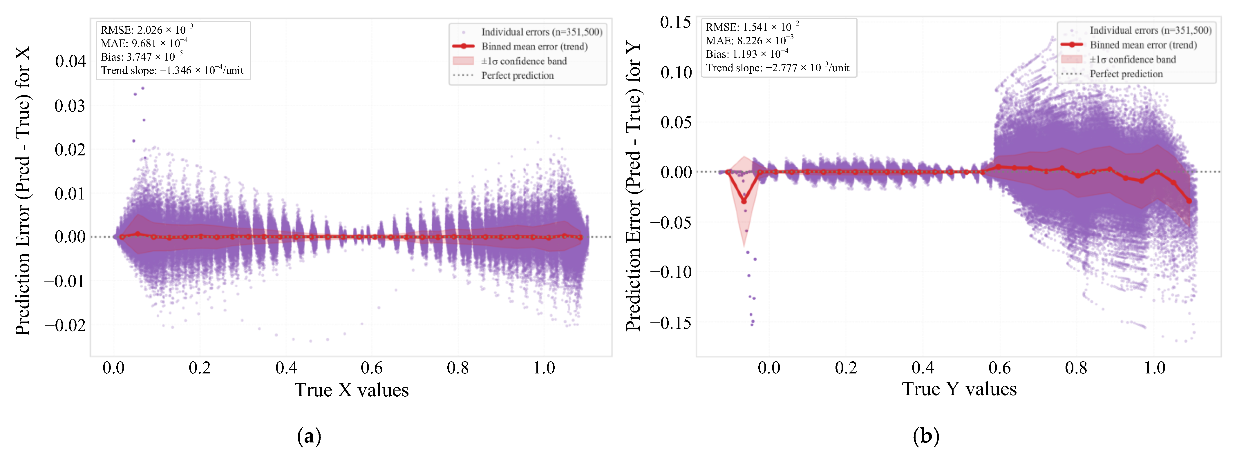
Figure 24 is used to test whether the model exhibits heteroscedasticity, i.e., whether the errors show systematic variation with the magnitude of the true values. Ideally, errors should be uniformly distributed around the zero line, independent of the true value magnitude. As shown in the figure, for both X and Y coordinates, the error points are uniformly distributed within a horizontal band. Furthermore, the binned mean error trend line calculated for intervals almost coincides with the zero-deviation line, with extremely small slopes (X: −1.346 × 10⁻⁴/unit, Y: −2.777 × 10⁻³/unit). This indicates that the model’s prediction error is a random variable independent of the true value, and there is no issue of prediction accuracy significantly degrading within specific numerical ranges. It signifies that the model possesses stable predictive performance across the entire design space. For engineering applications, its prediction results are generally trustworthy and not reliable only under specific numerical conditions.

6. Conclusions

Inspired by natural language processing models, this study adopts the sequence-to-sequence transformer model framework, combined with a self-attention mechanism and performance matching evaluation metrics, to propose a turbine cascade aerodynamic design optimization method. This method was validated in a typical turbine cascade, resulting in improved total pressure recovery coefficients and significantly enhanced curvature smoothness in key regions. The main conclusions of this study are as follows:
(1)
Compared to traditional “coordinate prediction” methods (such as CNN, MLP), the transformer model can capture complex nonlinear associations between curvature changes and geometric parameters, generating globally continuous blade coordinates. This method successfully suppressed non-physical solution phenomena in supersonic viscous flow fields, improved the uniformity of pressure gradients in the optimized blade profile, inhibited local flow separation, and provided a high-precision, low-computational-cost solution for the inverse design of turbine blade profiles.
(2)
CFD results show that the optimized blade profile has a thinner boundary layer in the acceleration zone and smoother flow acceleration, verifying the effectiveness of this method in local aerodynamic optimization. The suction surface velocity peak was reduced by 2.48%, the total pressure recovery coefficient increased from 0.949 to 0.954 (a relative improvement of 0.53%), and the total pressure loss coefficient decreased from 0.744 to 0.663, demonstrating comprehensive aerodynamic improvements.
(3)
This paper proposes a performance matching metric based on BERT embedding and cosine similarity, which achieves quantitative evaluation of the proximity between predicted blade profiles and target designs by mapping Mach number distributions to high-dimensional vectors and calculating cosine similarity. This metric can effectively reflect the model’s generalization ability and provide quantifiable feedback for design optimization directions.
(4)
Compared to the traditional CNN-CBAM model, the self-attention mechanism of the transformer model can avoid the field-of-view limitations of a CNN’s local convolution kernels. In key regions, the curvature smoothness of blade profiles generated by the transformer model is superior to that of CNN-CBAM.
(5)
Using the sequence-to-sequence transformer optimization method for aerodynamic optimization of a turbine cascade takes approximately 100 s, avoiding the multiple iterative correction processes of traditional modeling optimization and numerical simulations, improving design optimization precision and efficiency, and providing a new method for the intelligent optimization design of turbine blades.
Despite its advantages, the proposed method has several limitations. As a data-driven approach, its performance is constrained by the coverage of the training dataset and may not generalize beyond the learned design space without expanded data or continuous retraining. Moreover, the present study is limited to two-dimensional cascade profiles and focuses primarily on aerodynamic performance; extension to fully three-dimensional blades and the inclusion of structural and manufacturing constraints remain topics for future work.

Author Contributions

Conceptualization, S.X. and T.F.; methodology, S.X.; software, S.X.; validation, S.X., T.F. and S.Z.; formal analysis, T.F.; investigation, S.X.; resources, S.Z.; data curation, S.X.; writing—original draft preparation, S.X. and T.F.; writing—review and editing, S.X., T.F. and L.J.; visualization, S.X.; supervision, L.J.; project administration, L.J.; funding acquisition, L.J. All authors have read and agreed to the published version of the manuscript.

Funding

This research received no external funding.

Data Availability Statement

The data presented in this study are available upon request from the corresponding author.

Conflicts of Interest

The authors declare no conflicts of interest.

Nomenclature

Notations
a 1Inlet flow angle
bBoundary condition vector
CxBlade axial chord length
d, dk(Key/Query) vector dimension
DKLKullback–Leibler Divergence
Ma1Inlet Mach number
MaisIsentropic Mach number
Mpred (x)Mach number distribution of the model-predicted blade profile
Mture (x)Theoretically designed Mach number distribution
P*Total pressure
P2Outlet static pressure
PEPositional Encoding
posPosition in the sequence
Q, K, VQuery, Key, Value vectors in the attention mechanism
RleRadius of the blade leading edge
RteRadius of the blade trailing edge
T*Total temperature
vpred, vtureVectors of Mach number distributions after BERT embedding
x, yBlade geometric coordinates
βinInlet blade angle
βoutOutlet blade angle
γinInlet wedge angle
ξBlade unguided turning angle
Subscripts
inInlet parameter
outOutlet parameter
leLeading Edge
teTrailing Edge
predModel-predicted value
tureTrue/Designed value

Abbreviations

The following abbreviations are used in this manuscript:
BERTBidirectional encoder representation from transformers
CFDComputational fluid dynamics
CNNConvolutional neural network
FFNNFeedforward neural network
CBAMImproved convolutional block attention module
KLKullback–Leibler Divergence
LHSLatin Hypercube Sampling
MLPMulti-layer perceptron
MSEMean Squared Error
ReLURectified linear unit

References

  1. Bahrani, N. Multidisciplinary Design Optimization of Turbomachinery Blade. Master′s Thesis, University of Toronto, Toronto, ON, Canada, 2015. [Google Scholar]
  2. Wang, W.; Xiang, L.; Kang, E.; Xia, J.; Wang, C.; Yan, C. Multidisciplinary Design Optimization of Cooling Turbine Blade: An Integrated Approach with R/ICSM. Appl. Sci. 2024, 14, 4559. [Google Scholar] [CrossRef]
  3. Maral, H.; Alpman, E.; Kavurmacıoğlu, L.; Camci, C. A Genetic Algorithm Based Aerothermal Optimization of Tip Carving for an Axial Turbine Blade. Int. J. Heat Mass Transf. 2019, 143, 118419. [Google Scholar] [CrossRef]
  4. Zhang, W.; Li, L.; Li, Y.; Jiang, C.; Wang, Y. A Parameterized-Loading Driven Inverse Design and Multi-Objective Coupling Optimization Method for Turbine Blade Based on Deep Learning. Energy 2023, 281, 128209. [Google Scholar] [CrossRef]
  5. Hawthorne, W.R.; Wang, C.; Tan, C.S.; McCune, J.E. Theory of Blade Design for Large Deflections: Part I—Two-Dimensional Cascade. J. Eng. Gas Turbines Power 1984, 106, 346–353. [Google Scholar] [CrossRef]
  6. Tan, C.; Hawthorne, W.; McCune, J.; Wang, C. Theory of Blade Design for Large Deflections: Part II—Annular Cascades. J. Eng. Gas Turbines Power 1984, 106, 354–365. [Google Scholar] [CrossRef]
  7. Borges, J. A Three-Dimensional Inverse Method for Turbomachinery: Part I—Theory. J. Turbomach. 1990, 112, 346–354. [Google Scholar] [CrossRef]
  8. Zangeneh, M. A Compressible Three-Dimensional Design Method for Radial and Mixed Flow Turbomachinery Blades. Int. J. Numer. Methods Fluids 1991, 13, 599–624. [Google Scholar] [CrossRef]
  9. Demeulenaere, A.; Van Den Braembussche, R. Three-Dimensional Inverse Method for Turbomachinery Blading Design. J. Turbomach. 1998, 120, 247–255. [Google Scholar] [CrossRef]
  10. Dang, T. Evaluation of 3D Inverse Code Using Rotor 67 as Test Case; CR-1998-206994; Technical Report; NASA: Washington, DC, USA, 1998. [Google Scholar]
  11. Qiu, X.; Dang, T. 3D Inverse Method for Turbomachine Blading with Splitter Blades. In Proceedings of the ASME Turbo Expo 2000: Power for Land, Sea, and Air, Atlanta, GA, USA, 12–15 June 2000; ASME: New York, NY, USA, 2000; pp. 1–7. [Google Scholar]
  12. Thompkins, J.; Tong, S. Inverse or Design Calculations for Nonpotential Flow in Turbomachinery Blade Passages. J. Eng. Gas Turbines Power 1982, 104, 281–285. [Google Scholar] [CrossRef]
  13. Tong, S.; Thompkins, J. A Design Calculation Procedure for Shock-Free or Strong Passage Shock Turbomachinery Cascades. J. Eng. Gas Turbines Power 1983, 105, 369–376. [Google Scholar] [CrossRef]
  14. Arbabi, A.; Ghaly, W. Inverse Design of Turbine and Compressor Stages Using a Commercial CFD Program. In Proceedings of the ASME Turbo Expo 2013: Turbine Technical Conference and Exposition, San Antonio, TX, USA, 3–7 June 2013; ASME: New York, NY, USA, 2013; pp. 1–14. [Google Scholar]
  15. Ziegler, B. Adjoint Method-Based Inverse Design of Transonic Compressor Cascade with Boundary Layer Control. Prog. Comput. Fluid Dyn. 2017, 17, 335–343. [Google Scholar] [CrossRef]
  16. Zhu, Y.; Ju, Y.; Zhang, C. An Experience-Independent Inverse Design Optimization Method of Compressor Cascade Airfoil. Proc. Inst. Mech. Eng. Part A-J. Power Energy 2019, 233, 431–442. [Google Scholar] [CrossRef]
  17. Wang, D.X.; Li, Y.S. 3D Direct and Inverse Design Using NS Equations and the Adjoint Method for Turbine Blades. In Proceedings of the ASME Turbo Expo 2010: Power for Land, Sea and Air, Glasgow, UK, 14–18 June 2010; ASME: New York, NY, USA, 2010. GT2010-22049. pp. 1–9. [Google Scholar]
  18. Yang, J.; Liu, Z.; Shao, F.; Wu, H. Transpiration Boundary Condition Based on Inverse Method for Turbomachinery Aerodynamic Design: On the Solution Existence and Uniqueness. J. Propuls. Technol. 2015, 36, 579–586. [Google Scholar]
  19. Li, Y.; Chang, J.; Kong, C.; Bao, W. Recent Progress of Machine Learning in Flow Modeling and Active Flow Control. Chin. J. Aeronaut. 2022, 35, 14–44. [Google Scholar] [CrossRef]
  20. Li, Y.; Chang, J.; Wang, Z.; Kong, C. Inversion and Reconstruction of Supersonic Cascade Passage Flow Field Based on a Model Comprising Transposed Network and Residual Network. Phys. Fluids 2019, 31, 126102. [Google Scholar] [CrossRef]
  21. Jin, Y.; Li, S.; Jung, O. Prediction of Flow Properties on Turbine Vane Airfoil Surface from 3D Geometry with Convolutional Neural Network. In Turbo Expo: Power for Land, Sea, and Air; American Society of Mechanical Engineers: New York, NY, USA, 2019; p. V02DT46A007. [Google Scholar]
  22. Zhou, H.; Yu, K.; Luo, Q.; Du, W.; Wang, S. Design Methods and Strategies for Forward and Inverse Problems of Turbine Blades Based on Machine Learning. J. Therm. Sci. 2022, 31, 82–95. [Google Scholar] [CrossRef]
  23. Mai, J.; Li, Y.; Long, L.; Huang, Y.; Zhang, H.; You, Y. Two-Dimensional Temperature Field Inversion of Turbine Blade Based on Physics-Informed Neural Networks. Phys. Fluids 2024, 36, 037114. [Google Scholar] [CrossRef]
  24. Duta, M.C.; Duta, M.D. Multi-Objective Turbomachinery Optimization Using a Gradient-Enhanced Multi-Layer Perceptron. Int. J. Numer. Methods Fluids 2009, 61, 591–605. [Google Scholar] [CrossRef]
  25. Mansour, R.; Osama, S.; Ahmed, H.; Nasser, M.; Mahmoud, N.; Elkodama, A.; Ismaiel, A. Parametric Analysis Towards the Design of Micro-Scale Wind Turbines: A Machine Learning Approach. Appl. Syst. Innov. 2024, 7, 129. [Google Scholar] [CrossRef]
  26. Vaswani, A.; Shazeer, N.; Parmar, N.; Uszkoreit, J.; Jones, L.; Gomez, A.N.; Kaiser, Ł.; Polosukhin, I. Attention Is All You Need. arXiv 2017, arXiv:1706.03762. [Google Scholar]
  27. Fang, Y.; Reissmann, M.; Pacciani, R.; Zhao, Y.; Ooi, A.S.H.; Marconcini, M.; Akolekar, H.D.; Sandberg, R.D. Exploiting a Transformer Architecture for Simultaneous Development of Transition and Turbulence Models for Turbine Flow Predictions. In Turbo Expo: Power for Land, Sea, and Air; American Society of Mechanical Engineers: New York, NY, USA, 2024; p. V12CT32A023. [Google Scholar]
  28. Aulich, M.; Goinis, G.; Voß, C. Data-Driven AI Model for Turbomachinery Compressor Aerodynamics Enabling Rapid Approximation of 3D Flow Solutions. Aerospace 2024, 11, 723. [Google Scholar] [CrossRef]
  29. Hamakhan, I.A.; Korakianitis, T. Aerodynamic Performance Effects of Leading-Edge Geometry in Gas-Turbine Blades. Appl. Energy 2010, 87, 1591–1601. [Google Scholar] [CrossRef]
  30. Qi, Q.; Qin, K.; Huang, D. Effect of Streamwise Bionic Protuberances with Continuous Curvature Near the Leading Edge on Performance of Compressor Cascade Aerodynamics. Eng. Appl. Comput. Fluid Mech. 2025, 19, 2578015. [Google Scholar] [CrossRef]
  31. Pritchard, L.J. An Eleven Parameter Axial Turbine Airfoil Geometry Model. In Turbo Expo: Power for Land, Sea, and Air; American Society of Mechanical Engineers: New York, NY, USA, 1985; p. V001T03A058. [Google Scholar]
  32. Ji, L.; Ma, W.; Feng, F. Research on the Shock Wave Structure and Its Evolution in Turbine Cascades. Trans. Beijing Inst. Technol. 2015, 35, 571–575. [Google Scholar]
  33. Baldwin, B.; Lomax, H. Thin-Layer Approximation and Algebraic Model for Separated Turbulent Flows. In Proceedings of the 16th Aerospace Sciences Meeting, Reno, NV, USA, 16–19 January 1978; p. 257. [Google Scholar]
  34. Fei, T.; Ji, L.; Zhou, L. Application of Neural Network Model in Compressor Through-Flow Analysis. J. Aerosp. Power 2022, 37, 1260–1272. [Google Scholar]
  35. Fei, T.; Ji, L. Application of New Empirical Models Based on Mathematical Statistics in the Through-Flow Analysis. J. Therm. Sci. 2021, 30, 2087–2098. [Google Scholar] [CrossRef]
  36. Fei, T.; Ji, L.; Yi, W. Performance Characteristic Modeling for 2D Compressor Cascades. Int. J. Turbo Jet-Engines 2022, 39, 367–382. [Google Scholar] [CrossRef]
  37. Goldman, L.J.; Seashultz, R.G. Laser Anemometer Measurements in an Annular Cascade of Core Turbine Vanes and Comparison with Theory; Technical Report; NASA: Washington, DC, USA, 1982. [Google Scholar]
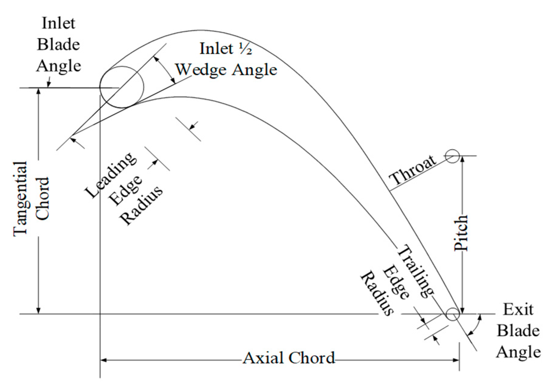
Figure 1. 11-parameter modeling method [31].
Aerospace 13 00052 g001
Figure 2. Partial blade profiles displayed in the dataset. The different colored lines represent three distinct blade profiles obtained via Latin hypercube sampling.
Aerospace 13 00052 g002
Figure 3. Computational mesh for a typical case.
Aerospace 13 00052 g003
Figure 4. Total pressure loss corresponding to different mesh quantities.
Aerospace 13 00052 g004
Figure 5. Mach number distribution corresponding to different mesh quantities.
Aerospace 13 00052 g005
Figure 6. Goldman cascade mesh.
Aerospace 13 00052 g006
Figure 7. Comparison of calculated and experimental Mach number distributions for the Goldman cascade.
Aerospace 13 00052 g007
Figure 8. Turbine blade optimization method based on sequence-to-sequence transformer model.
Aerospace 13 00052 g008
Figure 9. Schematic of KL divergence.
Aerospace 13 00052 g009
Figure 10. Performance matching metric.
Aerospace 13 00052 g010
Figure 11. CNN-CBAM structure.
Aerospace 13 00052 g011
Figure 12. Blade profile predicted by CNN-CBAM model.
Aerospace 13 00052 g012
Figure 13. Comparison of three Mach number distributions.
Aerospace 13 00052 g013
Figure 14. Comparison of Mach number contours between original blade profile and optimized blade profile.
Aerospace 13 00052 g014
Figure 15. Extraction positions of velocity at 11 locations along the blade surface.
Aerospace 13 00052 g015
Figure 16. Velocity distribution near the boundary layer at extraction positions.
Aerospace 13 00052 g016
Figure 17. Comparison between original and optimized blade profiles.
Aerospace 13 00052 g017
Figure 18. Comparison of Mach number distributions under different model parameters.
Aerospace 13 00052 g018
Figure 19. Comparison of performance matching degrees under different model parameters.
Aerospace 13 00052 g019
Figure 20. Comparison of blade profile geometries predicted by different models.
Aerospace 13 00052 g020
Figure 21. Histogram of curvature error distributions for different models.
Aerospace 13 00052 g021
Figure 22. Scatter plot comparing predicted values against true values: (a) X; (b) Y.
Aerospace 13 00052 g022
Figure 23. Distribution of prediction errors along the blade sequence positions.
Aerospace 13 00052 g023
Figure 24. Analysis of the relationship between prediction errors and true values: (a) X; (b) Y.
Aerospace 13 00052 g024
Table 1. Design blade profile parameters and ranges.
ParameterRange
Blade unguided turning, ξ (°)3.5~9.0
Inlet blade angle, βin (°)remain constant
Inlet wedge angle, γin (°)5.0~20.0
Radius of the blade leading edge, Rle (mm)0.05~0.10
Outlet blade angle, βout (°)remain constant
Radius of the blade trailing edge, Rte (mm)0.012~0.040
Blade axial chord, Cx (mm)30.0~40.0
Table 2. Boundary conditions.
Boundary ConditionsRange
Inlet total pressure, P 1 * (kPa)101.32
Inlet total temperature, T 1 * (K)288.15
Inlet flow angle, a 1 (°)32.6
Inlet mach number, Ma10.3
Outlet static pressure, P2 (kPa)40.0~90.0
Radius of the blade trailing edge, Rte (mm)0.012~0.040
Blade axial chord, Cx (mm)30.0~40.0
Note: * represents total conditions.
Table 3. Overall structural parameters of the transformer model.
ParameterValue/Description
Encoder–decoder layers5 layers
Layer compositionMulti-head attention, feedforward network, residual connection, layer normalization
Hidden nodes (encoder/decoder)512
Feedforward hidden nodes2048
Number of attention heads8
Dropout0.1
Input/target sequence processingEmbedding + positional encoding
Learning rate schedulerNoam scheduler
Overfitting mitigationLabel smoothing
OptimizerAdam
Table 4. Overall structural parameters of 1D-CNN-CBAM.
Layer NameStructural ParametersOutput SizeParameterValue/Description
Input Layer/1 × 308Encoder–decoder layers5 layers
Convolutional Layer C1CN = 32; CS = 1; stride = 132 × 308Layer compositionMulti-head attention, feedforward network, residual connection, layer normalization
Batch Normalization/32 × 308Hidden nodes (encoder/decoder)512
CBAM1/32 × 308Feedforward hidden nodes2048
Pooling Layer P1PS = 2; stride = 232 × 154Number of attention heads8
Convolutional Layer C2CN = 128; CS = 1; stride = 1128 × 154Dropout0.1
Batch Normalization/128 × 154Input/target sequence processingEmbedding + positional encoding
CBAM2/128 × 154Learning rate schedulerNoam scheduler
Pooling Layer P2PS = 2; stride = 2128 × 77Overfitting mitigationLabel smoothing
Convolutional Layer C3CN = 16; CS = 1; stride = 116 × 77OptimizerAdam
Batch Normalization/16 × 77
CBAM3/16 × 77
Pooling Layer P3PS = 2; stride = 216 × 38
Flatten/608 (16 × 38)
Fully Connected FC1/256
Fully Connected FC2/512
Fully Connected FC3/200
Output Layer/200
Note: CS and CN represent the convolution kernel size and number of convolution kernels, respectively; PS represents the pooling size.
Disclaimer/Publisher’s Note: The statements, opinions and data contained in all publications are solely those of the individual author(s) and contributor(s) and not of MDPI and/or the editor(s). MDPI and/or the editor(s) disclaim responsibility for any injury to people or property resulting from any ideas, methods, instructions or products referred to in the content.