Article

Advanced Implementation of the Asymmetric Distribution Expectation-Maximum Algorithm in Fault-Tolerant Control for Turbofan Acceleration

1
National Key Lab of Aerospace Power System and Plasma Technology, Xi’an Jiaotong University, Xi’an 710049, China
2
School of Mechanical Engineering, Xi’an Jiaotong University, Xi’an 710049, China
*
Author to whom correspondence should be addressed.
Aerospace 2025, 12(9), 829; https://doi.org/10.3390/aerospace12090829
Submission received: 7 August 2025 / Revised: 31 August 2025 / Accepted: 11 September 2025 / Published: 16 September 2025
(This article belongs to the Section Aeronautics)

Abstract

For the safety and performance of turbofan engines, the fault-tolerant control of acceleration schedules is becoming increasingly necessary. However, traditional probabilistic approaches struggle to satisfy the single-side surge boundary limits and control asymmetry. Moreover, the baseline fault-tolerance requirement of the acceleration schedule cannot depend on whether fault detection exists, and model-dependent data approaches inherently limit their generalizability. To address all these challenges, this paper proposes a probabilistic viewpoint of non-frequency and non-Bayesian schools, and the asymmetric distribution expectation-maximum algorithm (ADEMA) based on this viewpoint, along with their detailed theoretical derivations. The surge boundary enhances safety requirements for the acceleration control; therefore, simulations and verifications consider the disturbance combinations involving a single significant fault alongside normal deviations from other factors, including minor faults. In the event of such disturbances, ADEMA can effectively prevent the acceleration process from approaching the surge boundary, both at sea level and within the flight envelope. It demonstrates the smallest median estimation error (0.27% at sea level and 0.96% within the flight envelope) compared to other methods, such as the Bayesian weighted average method. Although its maintenance of performance is not exceptionally strong, its independence from model-data makes it a valuable reference.

1. Introduction

Safety is the primary concern during the turbofan acceleration process, which is ensured by the acceleration schedule [1]. The acceleration schedule aims to prevent high-pressure compressor (HPC) surge [2], and reserves a certain surge margin between itself and the theoretical surge boundary of the HPC to account for uncertainties [3], such as fuel metering errors, inlet flow distortion, deterioration and others [4]. Due to these uncertainties, it is often necessary to maintain a large surge margin (10~15% [5]), which significantly impacts the performance potential of the turbofan [6]. Therefore, implementing fault-tolerant control of the acceleration schedule is vital to achieving a balance between safety and performance. This approach enables the use of a lower surge margin design by accommodating the impact of certain disturbance factors.
The core technique of fault-tolerant control is redundancy configuration [7], which requires the acceleration controller to adopt various acceleration schedules. The commonly used strategies include a corrected fuel flow schedule [8] and a rotor speed derivative (N-dot) schedule [9,10,11]. In recent years, it is worth noting that Khalid et al. [12] unveiled a method of limiting a N-dot schedule with a corrected fuel flow schedule, which indicates a certain level of fault tolerance. In addition, a pressure ratio schedule can also be applied, but it is usually not the main option due to its susceptibility to sensor errors. The differentiation of these schedules based on their susceptibility to factors is beneficial in mitigating the impact of common-mode faults [7]. For example, the corrected fuel flow schedule is prone to being affected by fuel metering errors [13], whereas the N-dot schedule is sensitive to power extraction [14]. The corrected fuel flow schedule can be divided into two forms based on the different pressure sensor references [8,15]. In other words, a four-redundancy acceleration schedule strategy can be employed to effectively control the acceleration process. This idea was implemented using the multi-layer perceptron with exponential Gumbel loss (MLP-EGL) method in our previous paper [16], which demonstrates significant advantages compared to Khalid’s method. However, this method relies on fault data generated by a component-level model (CLM) that is not available in all engines. For broader engineering applications, it appears necessary to offer a model-free data learning method with simplicity. The four schedules ultimately output four fuel flow rates, so the essence of fault-tolerant algorithm design lies in how to fuse these four fuels. Due to the inverse relationship between real-time fuel flow rate and surge margin at the same speed, a smaller estimated result is more favorable than a larger one. This necessitates an asymmetric fuel distribution profile. The unilateral limitation of the surge boundary makes this problem distinct from conventional data fusion.
Conventional data fusion consistently optimizes for minimum variance during minor fault scenarios, an approach incompatible with our asymmetric needs [17]. For single significant faults, they treat deviations toward or away from the surge boundary with equal severity. What surprises us is that both the previous and current methods can be understood within the theoretical realm of recent modal regression to some extent [18]. Weixin Yao is one of the most influential researchers in this field. His theoretical foundation is local modal regression [19], and he introduced the modal linear regression model [20]. Another noteworthy researcher, Feng, proposed a loss function for modal regression [21], which is based on a Gaussian distribution. Liu et al. [18] and Wang et al. [22] exposed the robustness of modal regression. Liu et al. [23] attempted to unify modal regression within the Bayesian framework. Although these studies see the possibility of a unified theory, they have not completely clarified the essential differences between the probability idea of modal regression and the ideas based on the frequency and Bayesian schools. Building on a more suitable conceptual framework, this study’s methodology is inspired by the mode’s characteristics—including locality and robustness—as revealed in above researches. Due to the fact that estimating the local mode of the substantial probability significantly accommodates the introduction of asymmetry, the asymmetric distribution expectation-maximum algorithm (ADEMA) can effectively reduce the propensity toward the surge boundary.
The fault-tolerant control methods utilized in other fields of turbofan engines are either based on frequency or the Bayesian school, and have little effect on the fault-tolerant problem associated with acceleration schedules. For example, in the field of sensor fault-tolerant control, Li et al. [24] realized sensor fault diagnosis and signal reconstruction by applying estimated results based on the Kalman filter bank. Kalman filter is essentially the weighted average over time between measurable values and model-estimated values, typical of Bayesian thinking. The weighting is fundamentally derived from variance estimates. In our previous paper, we confirmed its limitations in accelerating transient processes [16]. Furthermore, Qiu et al. [25] developed the strategy of analytical redundancy logic and the dynamic adaptive calculation of the threshold, which reflects prior expectations. Some machine learning methods have also been introduced to the analytical redundancy design, such as selective updating regularized online sequential extreme learning machine [26] and Proper net methods [27]. In the field of actuator fault-tolerant control, Ma et al. [28] developed a virtual actuator control strategy to correct the input of the actuator under the simultaneous actuator fault and sensor fault, while Cheng et al. [29] even applied convolution neural network to actuator fault diagnosis, which is combined with a nonlinear fault-tolerant control for reducing the accuracy requirements of the actuator. These essentially weighted-average-based methods have limited control over the output distribution’s symmetry. The fault-tolerant control of sensors or actuators cannot completely prevent the transmission of error effects to the controller, so the control schedules of the turbofan also need a fault-tolerant design to some extent. For the steady control, Ring et al. [30] provided four control modes of the turbofan to tolerant multiple sensor faults with only minor control impact. For the transient control, Peng et al. [31] applied an N-dot schedule as the reconstruction of the start control law when the exhaust temperature sensor fails. The above methods predominantly rely on the concept of switching or compensation, which requires additional fault detection. However, GJB10890-2023 requires that the acceleration schedule itself must maintain fault tolerance—regardless of detectability [32]. These are exactly the two main reasons why the previous methods are challenging to apply to fault-tolerant control problems in acceleration schedules.
The main contributions of this paper are summarized as follows:
(1)
This paper proposes a theoretical viewpoint of substantial probability, which constitutes the foundation of fault-tolerant control methods for turbofan engine acceleration schedules. This discovery presents significant theoretical progress in probability theory.
(2)
This paper derives the iterative formulas of ADEMA applicable for fault-tolerant control in acceleration schedules, relying solely on the real-time fuel output from the four schedules and their cumulative variances.
Compared to the minimum variance-based methods commonly used in data fusion, the ADEMA proposed in this study not only maintains considerable accuracy but also systematically biases the estimates in a specific direction.

2. Probability Bases of Methods

2.1. Viewpoint of Frequency School

The frequency school assumes that the samples are independent and identically distributed, and requires that the following optimization objective be met:
arg max μ   p x 1 , x 2 , , x n = arg max μ i = 1 n p x i
where xi is the i-th sample random variable of the original random variable x, and μ is the expectation or parameter to be learned.
If all these samples follow a Gaussian distribution, Equation (1) can be transformed into determining the logarithmic maximum likelihood probability:
p x i = 1 2 π σ exp 1 2 x i μ σ 2
arg max μ ln i = 1 n p x i = arg max μ i = 1 n 1 2 x i μ σ 2 ln 2 π σ arg min μ i = 1 n x i μ 2
where σ is the standard deviation in general.
Therefore, the most commonly used L2 (or mean squared error) loss function can be obtained as follows:
L μ , x i = μ x i 2
where μ can be a constant or replaced with the model output value, and xi can be an independent sample value or replaced with the true output value corresponding to the sampled input.
Similarly, if the sample distribution is assumed to be a Laplace distribution, the L1 (or mean absolute error) loss function can be derived; if the sample distribution is assumed to be a Gumbel distribution, the linear exponential (Linex) loss function can also be derived [33].
If the derivative of the total loss in Equation (3) with respect to μ is set to 0, the analytical solution for the extremum can be obtained as follows:
arg min μ   J μ = arg min μ i = 1 n x i μ 2 d J d μ = i = 1 n 2 x i μ = 0 μ = 1 n i = 1 n x i
It can be seen that regression fitting based on L2 loss function is equivalent to calculating the sample mean.

2.2. Viewpoint of Bayesian School

The Bayesian school maintains a strong skepticism, asserting that seemingly unconditional probabilities actually hide underlying conditions. Hence, Equation (1) should be adjusted as follows:
arg max μ   p x 1 , x 2 , , x n μ = arg max μ i = 1 n p x i μ
That is to say, from the viewpoint of the Bayesian school, the frequentist aims to determine which expectation maximizes the likelihood of the current sample combination appearing, without focusing on the expectation itself. In fact, if there is an original random variable x, it may not necessarily yield this existing combination.
Thus, the optimization objective of the Bayesian school is to maximize the posterior probability. The Bayesian approach not only requires that the expectation has explanatory power for the current samples, but also for other possible samples that have not yet appeared.
p μ x 1 , x 2 , , x n p x 1 , x 2 , , x n = p x 1 , x 2 , , x n μ p μ
arg max μ   p μ x 1 , x 2 , , x n
If p(x1, x2, …, xn) is assumed to be constant, then the logarithmic version of objective (8) has the following form:
arg max μ ln p μ x 1 , x 2 , , x n arg max μ ln i = 1 n p x i μ p μ
The Bayesian school assumes that p(μ) follows a prior or subjective probability distribution, so we can further assume that both the sample distribution and p(μ) satisfy Gaussian distributions.
p μ = 1 2 π σ 0 exp 1 2 μ μ 0 σ 0 2
The logarithmic maximum likelihood of the posterior probability can be concretized into the following form:
arg max μ ln i = 1 n p x i μ p μ = arg max μ i = 1 n 1 2 x i μ σ 2 ln 2 π σ 1 2 μ μ 0 σ 0 2 ln 2 π σ 0 arg min μ i = 1 n x i μ 2 + σ σ 0 2 μ μ 0 2
For convenience, the following definition is made:
λ = σ σ 0 2
Therefore, the total loss of the Bayesian school is equivalent to the total loss of the frequency school plus L2 regularization.
Similarly, if the derivative of the total loss in formula (11) with respect to μ is set to 0, the analytical solution for the extremum can be obtained as follows:
arg min μ   J μ = arg min μ i = 1 n x i μ 2 + λ μ μ 0 2 d J d μ = i = 1 n 2 x i μ + 2 λ μ μ 0 = 0 μ = n n + λ 1 n i = 1 n x i + λ n + λ μ 0
Therefore, it is interesting that the Bayesian school actually exhibits a stronger pragmatic tendency by introducing the subjective expectation or prior knowledge. Even in a narrower sense, μ0 only represents the sample mean based on past experiences (that is, λ is the experience number), but it still carries a significant empirical color.

2.3. Viewpoint of Non-Frequency and Non-Bayesian Schools

It can be assumed that p(xi) and p(μ) are constants, simplifying the sample random variable to one. Hence, a Bayesian formula can be expressed as shown in Equation (15).
p μ x i p x i = p x i μ p μ
p μ x i = c o n s t × p x i μ
If both sides of the equation satisfy Gaussian distributions:
1 2 π σ exp 1 2 μ x i σ 2 = 1 2 π σ exp 1 2 x i μ σ 2
where on the left side of Equation (16), μ is the random variable and xi is the specific expectation value, while on the right side, it is the opposite.
In so far as both μ and xi represent expectations, their values are essentially the same. In so far as they are both random variables, there is no difference whether they are labeled as μ or xi. This is completely a tautology. Therefore, we do not consider xi as an actual random variable; it is purely an expectation of the conditional probability of x given μ = xi, as expressed in Equation (17). Each sample value is sampled because it has the highest probability under the specific conditions.
p x μ = x i = 1 2 π σ exp 1 2 x x i σ 2
p(x) can be regarded as a marginal probability distribution:
p x = p x μ p μ d μ
Within the realm of rational numbers, p(x) can be expressed in discrete form, which might be considered as the original division between probability and statistics.
p x = i = 1 n p x μ = x i P μ = x i
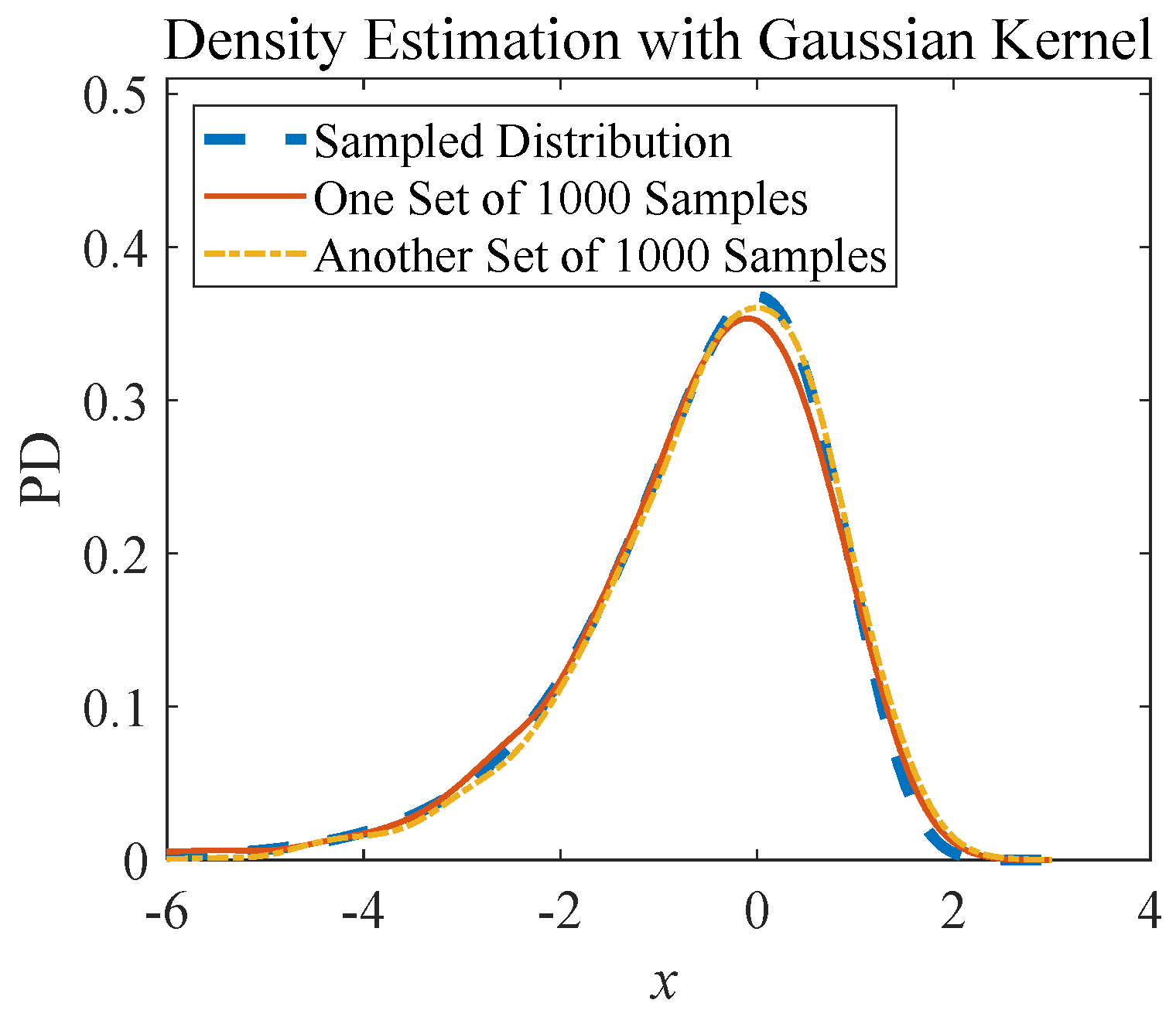
If we assume that P(μ = xi) follows the principle of equal probability, we can derive the equation for probability density estimation, as expressed in Equation (20). Hence, Equation (17) is the Gaussian kernel function [34].
p x = 1 n i = 1 n p x μ = x i
Therefore, in addition to the frequency and Bayesian schools, another optimization objective is to optimize the substantial probability p(x).
arg max x   p x
Thus, the modal loss function is essentially the inverse of a convex probability distribution. The modal loss function of the Gaussian distribution can be expressed in the form shown in Equation (22).
L x , x i = 1 exp 1 2 x x i σ 2
Therefore, the loss function designed in our previous paper was a negative expression of the Gumbel distribution as shown in Equation (23), but the corresponding proof based on the viewpoint of frequency school was still clumsy [16].
L x , x i = 1 exp x x i σ exp x x i σ + 1
The comparison between the loss functions of the frequency (or Bayesian) school and the loss functions of modal regression under the assumption of the same probability distributions is illustrated in Figure 1.
Optimizing Equation (21) yields the sample mode. The maximum of substantial probability p(x) can be achieved through iterative formulas using the EMA [20,35].
p(x) can be decomposed in countless ways to accommodate various combinations of samples. Conversely, different combinations of samples can result in the same p(x), as illustrated in Figure 2. That is why it is substantial. Indeed, p(x) itself may also imply conditions, requiring some samples to be explained, leading to a more substantial probability. If Mode is the mode of p(x), then there can also be a substantive probability p(x|μ = Mode).

3. Background of Fault-Tolerant Control for Turbofan Acceleration

Before mathematizing the problem and deriving the formulas for ADEMA, it is still necessary to introduce the background and symbolization of the four schedule fuels. The object of discussion here is a hybrid exhaust turbofan engine, whose stage definitions are shown in Figure 3. HPT and LPT are high-pressure turbines and low-pressure turbines, respectively.
The turbofan acceleration process is mainly limited by the surge boundary of HPC, and the acceleration schedule is used to meet this requirement. Thus, the methodology derived herein is also applicable to other core-engine-based propulsion systems. The acceleration schedule should reserve a certain surge margin to adapt to the impacts of intake distortion, degradation, etc. Common surge margin design values for acceleration schedules include 11% [4], 12.4% [2], 15% [5] and so on. In this paper, a lower surge margin design of 7.3% will be adopted. The following is the definition formula for the surge margin [36]:
S M C = π C W a , cor S π C W a , cor O 1 N H , cor × 100 %
where SMC is the surge margin of HPC, πC is the pressure ratio of HPC, Wa,cor is the corrected air mass flow of HPC inlet, S denotes the surge boundary point, O denotes the current operating point, and NH,cor denotes the identical corrected high-pressure rotor speed for S and O.
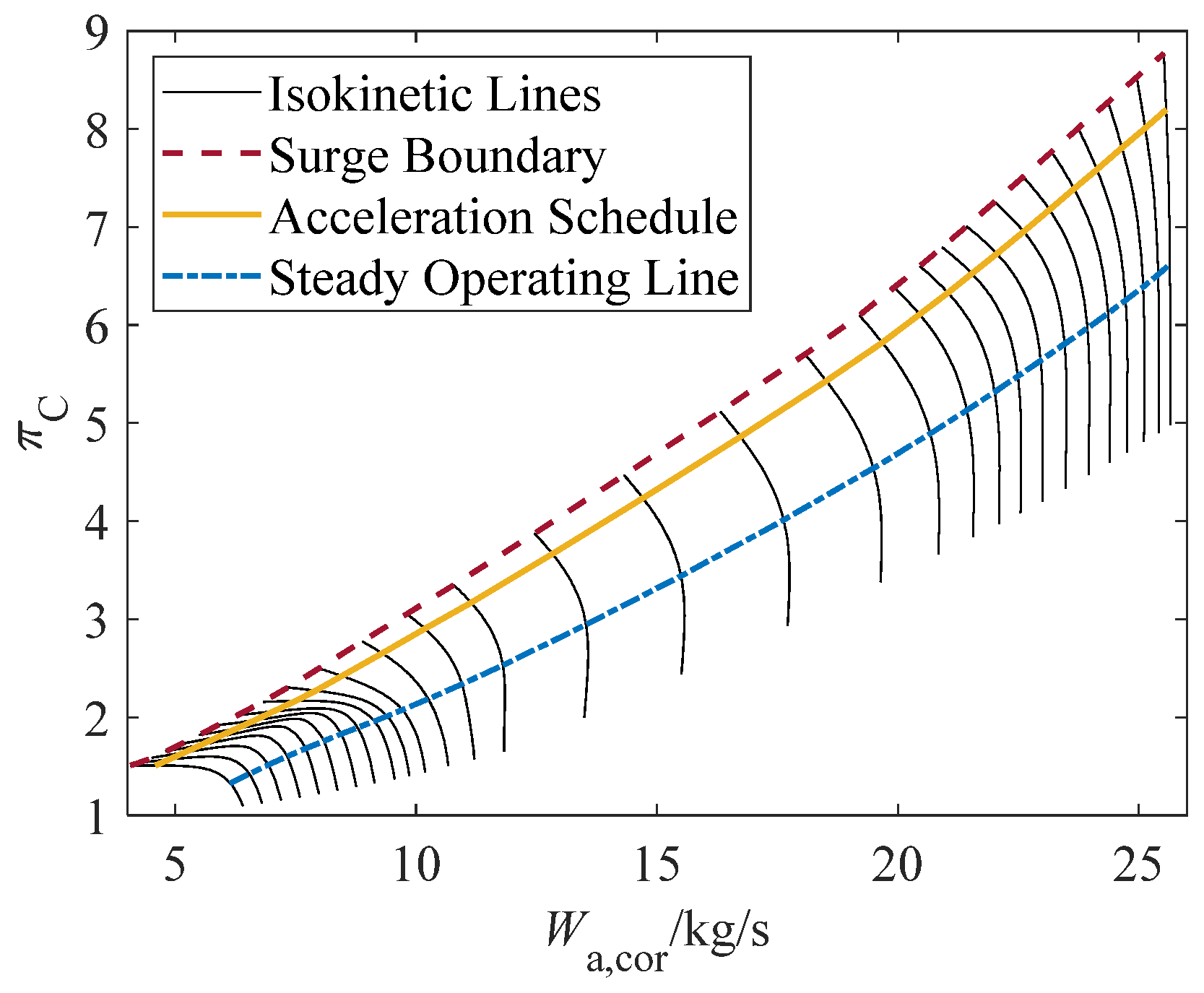
The position of the acceleration schedule in terms of component characteristics of the HPC is shown in Figure 4. The thin solid lines from left to right represent the isokinetic lines from low to high, indicating the relationships between πC and Wa,cor at the same NH,cor.
The SMC cannot be measured directly and is usually constrained by controlling other related parameters, such as the corrected fuel flow, the corrected speed derivative, and πC. There are two forms of corrected fuel flow based on the differences in reference pressure sensors, resulting in four possible schedules, as follows:
n H , cor = N H T t 25 , ref / T st N H , ref T t 25 / T st
n H , cor 2 = N H N H , ref T t 2 / T st
π C = φ 1 n H , cor
W f , cor 2 = W f p t 2 / p st T t 2 / T st 0.7 = φ 2 n H , cor 2
W f , cor 31 = W f p t 31 / p st T t 2 / T st 0.7 = φ 3 n H , cor 2
N d o t cor = N ˙ H p t 25 / p st 1.1 T t 2 / T st 0.7 = φ 4 n H , cor 2
where NH is the high-pressure rotor speed, NH,ref is the constant reference speed of NH, Tt25,ref is the constant corresponding reference temperature, and Tst and pst is the standard atmosphere temperature and pressure at sea level, respectively; Tt2 and pt2 is the total temperature and pressure of stage 2, respectively, Tt25 and pt25 is the total temperature and pressure of stage 25, respectively, and pt31 is the total pressure of stage 31; nH,cor denotes the relative corrected NH based on Tt25, nH,cor2 denotes the relative corrected NH based on Tt2, Wf,cor2 denotes the corrected fuel flow based on pt2, Wf,cor31 denotes the corrected fuel flow based on pt31, and Ndotcor denotes the corrected speed derivative.
These four schedules must be activated through the Accel Controller in the main fuel control architecture, as shown in Figure 5. Their objectives may differ, but the controllable variable remain the same, i.e., main fuel flow Wf. The final Wf provided to the actuator is determined as the minimum value between the fuel flow derived from the Accel Controller (Wf,acc) and the comparison result from other sources. The comparison result is obtained from a process in which the speed PID control output fuel (Wf,PID) first takes the minimum value with the output fuel (Wf,res) of the Restriction Controller (which includes overspeed, overtemperature, and overpressure), and then takes the maximum value with the output fuel Wf,dec of the Decel Controller. In short, the Accel Controller typically plays a dominant role only during the mid-phase of the acceleration process.
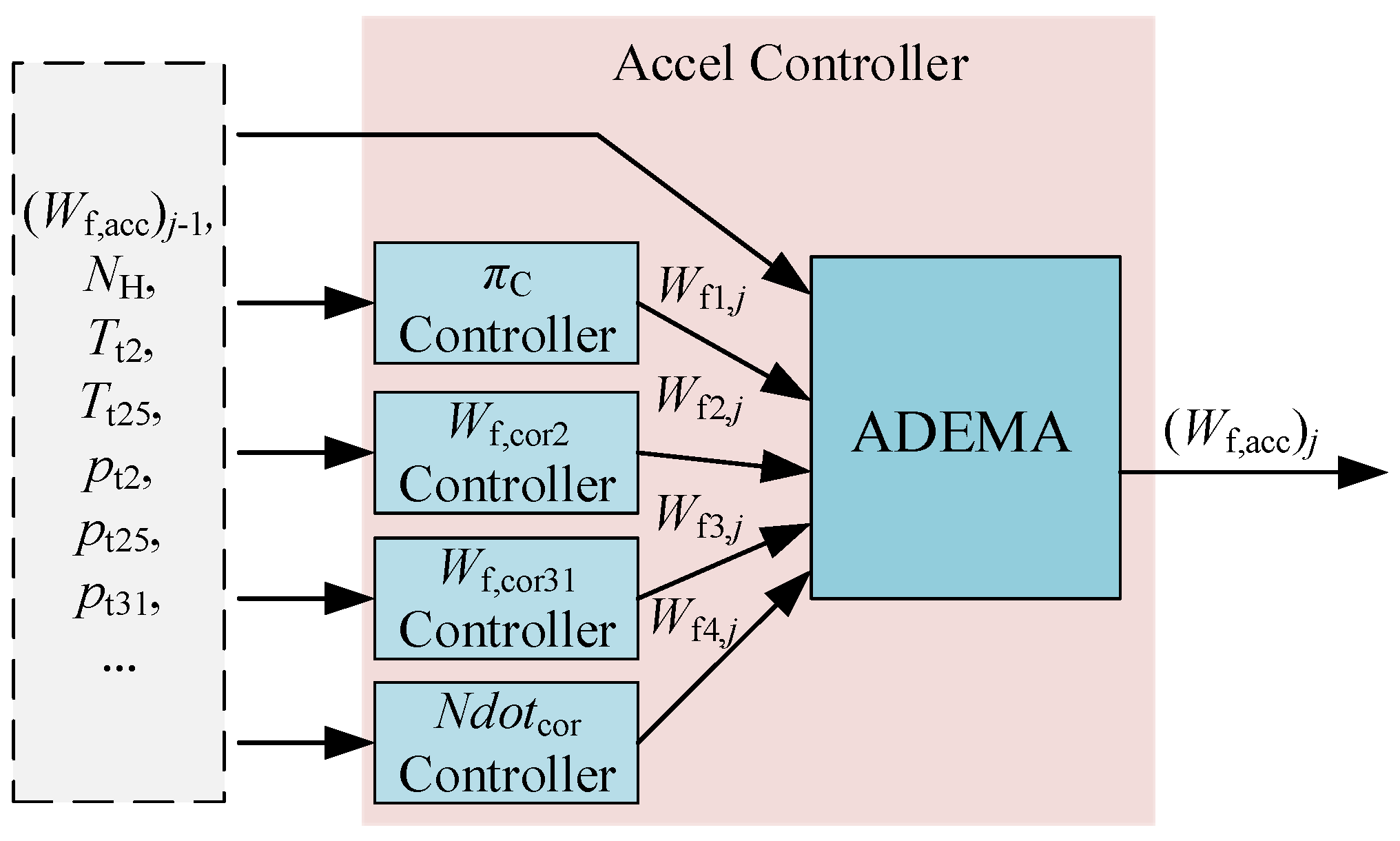
The control programs of the four schedules also needs to be configurated in the Accel Controller. The controllers associated with the four schedules consistently provide four distinct fuel flow rates (Wf1,j, Wf2,j, Wf3,j, Wf4,j) at any given time j. Consequently, the ADEMA is tasked with estimating the appropriate acceleration fuel flow output (Wf,acc)j based on these four fuels at each time j, as illustrated in Figure 6. Due to the inverse relationship between real-time fuel flow rate and surge margin at the same speed, a smaller estimated result is more favorable than a larger one for avoiding surge. This necessitates an asymmetric fuel distribution profile.
This section still needs to identify the fault factors that must be considered for validation. The general accuracy of the main measurement types in the turbofan is shown in Table 1.
According to ISO 2314:2009(E), the standard deviation of measurands can be calculated by dividing the calibration numerical value by 2 [37]. For example, the standard deviation of fuel flow is 0.5%. However, the standard deviation of “normal deviation”, as defined in the previous paper, equals the calibration numerical value, implying that the definition range encompasses the possibility of minor faults. Table 2 presents the “normal deviation” and significant fault ranges of the considered disturbance factors. The fault-tolerant design goal is to ensure acceleration safety and performance stability amidst a single significant fault and normal deviations from other factors (including minor faults). This verification aims to prevent excessive sensitivity of the final estimation results to a single disturbance factor. The accuracy of the speed sensor is typically extremely high, with minimal truncation error, and is, hence, disregarded [38]. Low-pressure component characteristics minimally affect the SMC, leading to considerations limited to HPC and HPT cases. The normal deviations of healthy parameters reflect engine-to-engine variation [39], with significant fault cases treating changes in efficiency and flow capacity of a single component as a single fault. In each disturbance combination, the factor that serves as a significant fault is randomly selected. The standard deviation of a significant fault or normal deviation is 1/3 of its range in Table 2, using a Gaussian distribution for sampling, with 1/10 of the normal deviation’s standard deviation defined as the standard deviation for white noise. Given the acceleration controller’s brief dominant time, these disturbance combinations are assumed to manifest as step signals from the start of acceleration.
Table 2. The normal deviation and the fault ranges of the disturbance factors [16].
Disturbance Factor *Normal DeviationSignificant Fault
Lex[0, 100 kW]∙(nH,Cor2)2Extra [0, 200 kW]
pt2 sensor[−1.5%, 1.5%]±[1.5%, 15%]
pt25 sensor[−1.5%, 1.5%]±[1.5%, 15%]
pt31 sensor[−1.5%, 1.5%]±[1.5%, 15%]
Wf metering[−3%, 3%]±[3%, 21%]
Tt2 sensor[−0.6%, 0.6%]±[0.6%, 6%]
Tt25 sensor[−0.6%, 0.6%]±[0.6%, 6%]
ΔSEC[−0.2%, 0.2%]Extra [−2%, 0]
ΔSWC[−0.2%, 0.2%]Extra [−4%, 0]
ΔSEHT[−0.2%, 0.2%]Extra [−2%, 0]
ΔSWHT[−0.2%, 0.2%]Extra [−2%, 2%]
* Lex denotes the power extraction, ΔSEC, ΔSEHT denotes the isentropic efficiency variations in HPC and HPT, and ΔSWC, ΔSWHT denotes the flow capacity variations in HPC and HPT.

4. ADEMA Derivation

It is found that N-dot control using the relative value of fuel increment is more conducive to the effectiveness of ADEMA. Hence, it is adopted here. Control objectives for the acceleration schedules, detailed in Formulas (27)–(30), are dependent on rotational speed. To mitigate speed’s impact, the four fuels are represented as relative values, as expressed in Equation (31). However, if the number of non-relative increments of PI control in the schedules is greater than other types, adopting the absolute value form is preferable.
x i , j = W f i , j W f , acc j 1
where i denotes different acceleration schedules, and j denotes the discrete time.
Correspondingly, the relative value of the acceleration fuel flow output at this moment is defined as follows:
x j = W f , acc j W f , acc j 1
Therefore, the fault-tolerant problem of acceleration schedules can be transformed into a probability problem now, that is to say, how can the random variable xj based on samples xi,j exhibit a downward-biased asymmetric distribution, with its statistic (median or mode) close to the ideal value. The best situation is not to have an upward long tail. However, fuel and surge margin are only negatively correlated, and their mutual influence between distributions still needs further research. Another possible factor that affects the effectiveness of this mathematical transformation is the accuracy of the acceleration schedules themselves. These issues have to be assumed to have no significant impact on the turbofan here. Anyway, from the viewpoint of substantial probability, the solution is to optimize the substantial probability.
According to the approximate definition of substantial probability, there is the following equation:
p x j = i = 1 m p x j μ = x i , j P μ = x i , j
where m denotes the total number of different schedules, and here it is 4.
For convenience, Equation (33) is simplified as follows:
p x j = i = 1 m p x j z = i P z = i
where z denotes the selected one among the different schedule fuel condition distributions.
According to the Bayesian formula, there is the following substitution relationship:
P z = i = p x j P z = i x j = p x j , z = i
The optimization objective of the ADEMA derivation is also transformed into logarithmic form as follows:
arg max x j ln p x j
The general derivation process of EMA or ADEMA is as follows:
ln p x j = ln p x j i = 1 m P z = i = ln p x j , z = i P z = i x j i = 1 m P z = i = i = 1 m P z = i ln p x j , z = i P z = i ln P z = i x j P z = i = i = 1 m P z = i ln p x j , z = i P z = i i = 1 m P z = i ln P z = i x j P z = i = E L B O x j + D KL P z = i P z = i x j
where ELBO(∙) denotes the evidence lower bound, and DKL(∙) denotes the Kullback–Leibler divergence.
According to the Jensen inequality, there is the following relationship:
ln p x j E L B O x j
If P(z = i) = P(z = i|xj), then the equality sign in inequality (38) holds, that is, indicating that maximizing ln p(xj) is equivalent to maximizing ELBO(xj). However, this equality does not hold most of the time. Hence, we have to prescribe P(z = i) = P(z = i|xj) given a known xj to make the equal sign temporarily hold, derive a new xj, and iterate this process until xj no longer updates. From a Bayesian perspective, this iterative process is endless, whereas under the substantial probability framework, it terminates. Convergence depends on the inequality constraint. Therefore, ADEMA comprises two primary steps: E-step and M-step.
  • E-step;
xj is a known quantity (including the preset initial value and last optimized results); therefore, the posterior probability can be obtained as follows:
γ i , j = P z = i x j = p x j z = i P z = i p x j = p x j z = i P z = i i = 1 m p x j z = i P z = i
2.
M-step.
Let P(z = i) = P(z = i|xj), and let the derivative of ELBO(xj) with respect to xj be 0, to obtain a new xj.
ln p x j = E L B O x j = i = 1 m γ i , j ln p x j z = i P z = i γ i , j
d E L B O d x j = 0 x j new
In the E-step, the xj is given as a known parameter; in the M-step, it is once again an unknown random variable to be solved, and it becomes a known parameter in the result (xj)new, repeating the cycle. That is why the E-step is called the expectation-step and the M-step is called the maximization-step (or maximum-step).
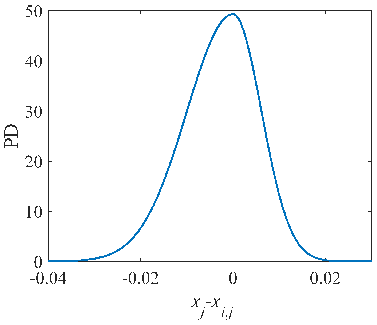
If p(xj|z = i) is assumed to follow a Gaussian distribution here, the classical EMA iteration formula can be obtained. However, as we already know, the fuels derived from the acceleration schedules are easily influenced by disturbance factors and tend towards the surge boundary. Therefore, we need to adopt an asymmetric distribution assumption. This immediately leads to consideration of the Gumbel distribution, but it is difficult to obtain a simple analytical formula. Logarithmic probabilities are clearly advantageous for the derivation of the Gaussian distribution. Therefore, an asymmetric Gaussian distribution seems necessary.
h i , j = σ j , x j x i , j c A σ j , x j > x i , j
p x j z = i = 2 1 + c A 1 2 π σ j exp 1 2 x j x i , j h i , j 2
where cA is the asymmetric coefficient for the deviation, and 0 ≤ cA ≤ 1; σj is the left half standard deviation at time j; the integral of this distribution across its full domain evaluates to unity.
If σj = 0.01 and cA = 0.618, the function graph of the distribution is shown in Figure 7.
Based on the asymmetric Gaussian distribution, we can further derive the corresponding xj iteration formula as follows:
d E L B O d x j = i = 1 m γ i , j x j x i , j h i . j 2 = 0 x j = i = 1 m γ i , j h i . j 2 x i , j / i = 1 m γ i , j h i . j 2
If cA = 1, the iteration formula for the symmetric Gaussian distribution can be obtained as follows:
x j = i = 1 m γ i , j x i , j
It is evident that solving for the sample mode involves an iterative weighted average process. Prior to the formal implementation of the ADEMA method, several parameter-setting issues still require resolution. The most commonly used estimation method for parameter σj is as follows:
x ¯ j = 1 m i = 1 m x i , j
σ j = 4 3 m 1 5 × 1 m 1 i = 1 m x i , j x ¯ j 2
However, in practical use, using the interquartile range instead of the sample standard deviation is more reliable:
σ j = 4 3 m 1 5 × Q 1.34
where Q is the interquartile range, and for four samples, it is approximately equivalent to subtracting the second smallest value from the third smallest value.
However, Silverman’s robust method is to take the minimum of the two, which takes the following specific form [34]:
σ j = 0.9 × 1 m 1 5 × min 1 m 1 i = 1 m x i , j x ¯ j 2 , Q 1.34
The parameter cA is typically chosen as 0.618 based on experience with fault-tolerant applications in acceleration schedules. Given the limited sample size of only 4, P(z = i) no longer relies on the assumption of equal probabilities but instead employs a variance estimation method outlined in Equations (50)–(52). Our current procedure involves updating the probabilities every time n accumulates to 30,000 and then recounting them.
d i , j = x i , j x ¯ j , x i , j x ¯ j c D x i , j x ¯ j , x i , j < x ¯ j
v i = 1 n j = 1 n d i , j 2
P z = i = 1 / v i i = 1 m 1 / v i
where cD is the deviation coefficient, and based on experience, it usually chooses 0.618 for these four schedules.
The last issue is the selection of the initial value (xj)0 for iteration. The initial value we adopted is the second smallest sample value rather than the average value, in order to prevent the result from converging to the larger side when a multimodal distribution occurs. Using the minimum value as the initial value is feasible, but it reduces iterative efficiency. If m is not 4 or considering other special conditions such as low design accuracy, take the smallest or second smallest value as the initial value. The basic steps of ADEMA can be described in Algorithm 1, relying solely on the real-time fuel output from the four schedules and their cumulative variances.
Algorithm 1 ADEMA method.
Input:
Relative values of four acceleration schedule fuels: xi,j;
Initial value of relative acceleration fuel output at time j: (xj)0;
Probabilities of not being updated yet or their initial presuppositions: ωi = P(z = i);
Set the coefficient cA;
The iteration step initialization: k = 0.
Process:
1. Calculate hi,j according to Equation (42), and refer to Equation (49) for σj;
2. Calculate γi,j according to Equation (39), and refer to Equation (43) for distribution;
3. k = k + 1, and calculate the new (xj)k according to Equation (44);
4. Repeat the above steps until the error |(xj)k−(xj)k-1| is less than the set value ε (like 0.001);
5. Calculate (Wf,acc)j based on the final (xj)end;
6. Refer to Equation (52) to check whether ωi needs to be updated.
Output:
Output the final acceleration fuel flow at time j: (Wf,acc)j.

5. Verification Results

5.1. Operation Test Under Simple Fault Conditions
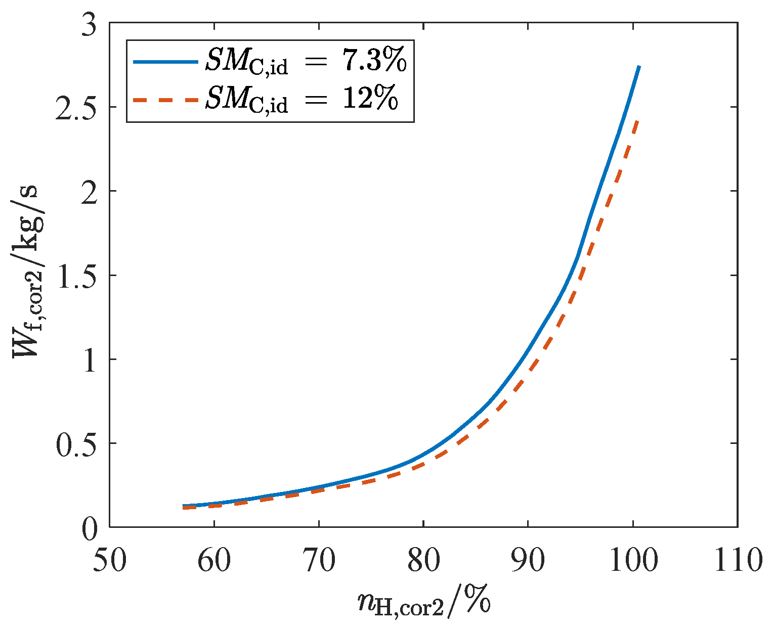
At first, the advantage of low margin design is verified based on a CLM, which has been validated with actual test data and has high accuracy [40,41]. SMC,id denotes the designed surge margin. Taking Wf,cor2 schedule as an example, the difference between a 7.3% SMC,id and a 12% SMC,id is illustrated in Figure 8.
Figure 8. The Wf,cor2 schedules of SMC,id = 7.3% and SMC,id = 12%.
Aerospace 12 00829 g008
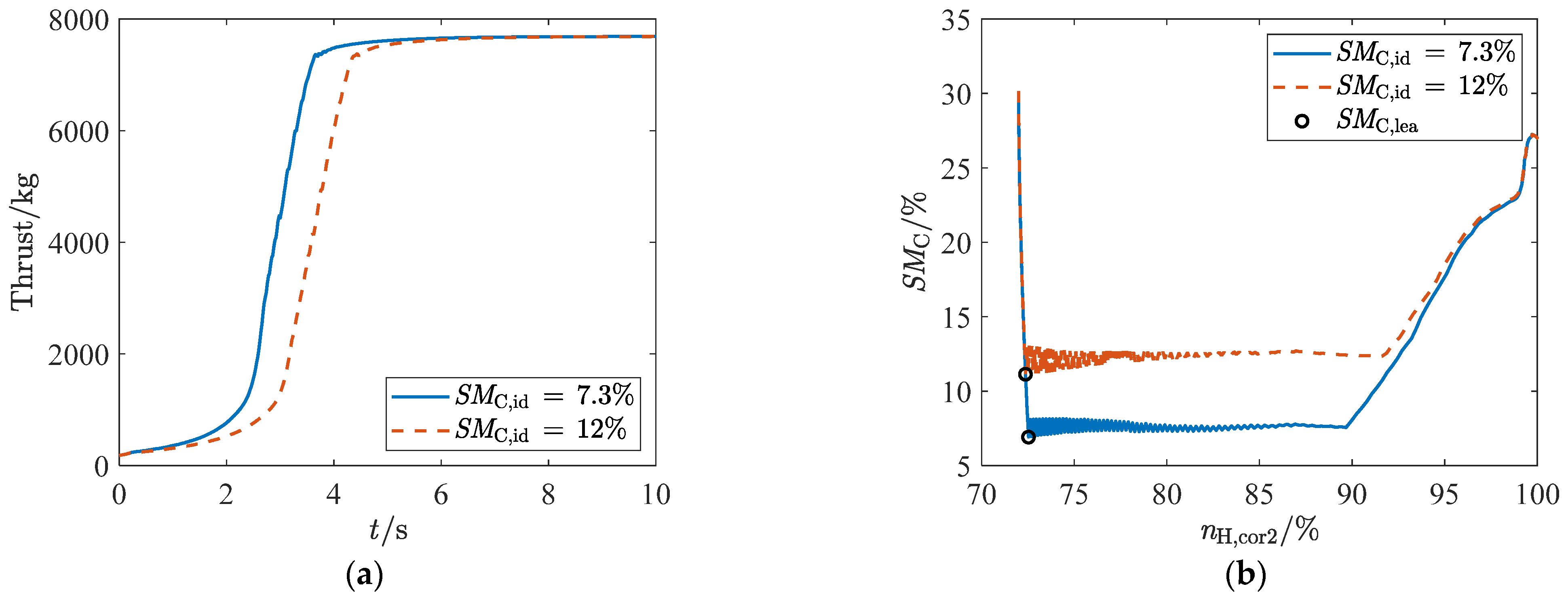
The effects of two SMC,id designs controlling full acceleration are presented in Figure 9. Full acceleration refers to the process from an idle state (nH,cor2 = 72% at sea level) to an intermediate state (nH,cor2 = 100% at sea level) under a step command initiated by the throttle lever. The full acceleration time is the time that achieves 95% target thrust change [42]. The full acceleration times of the 7.3% SMC,id and 12% SMC,id are 3.64 s and 4.36 s, respectively, that is, the former is about 16.5% less than the latter. Although Wf,cor2 schedules can maintain SMC near the design objective under normal operation conditions, all single schedules is difficult to withstand the impact of a single significant fault [16]. The least surge margin experienced during each acceleration process is denoted by SMC,lea, which is a focus of our verification.
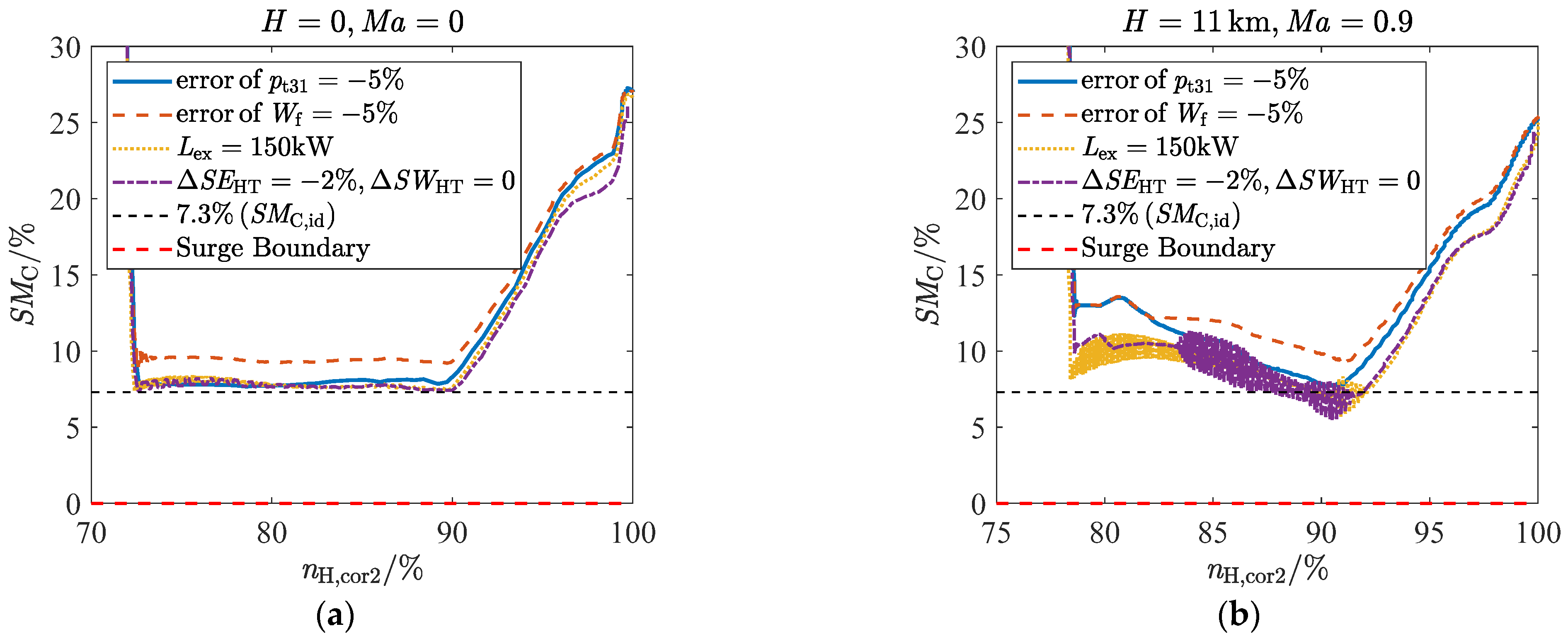
Under a single significant fault condition, the effects of ADEMA in controlling the acceleration process at sea level (H = 0, Ma = 0) and an envelope point (H = 11 km, Ma = 0.9) based on the hardware-in-the-loop (HIL) platform are shown in Figure 10. The results indicate that it can effectively prevent the acceleration process from approaching the surge boundary (SMC = 0) and maintain it as close as possible to a 7.3% SMC,id.
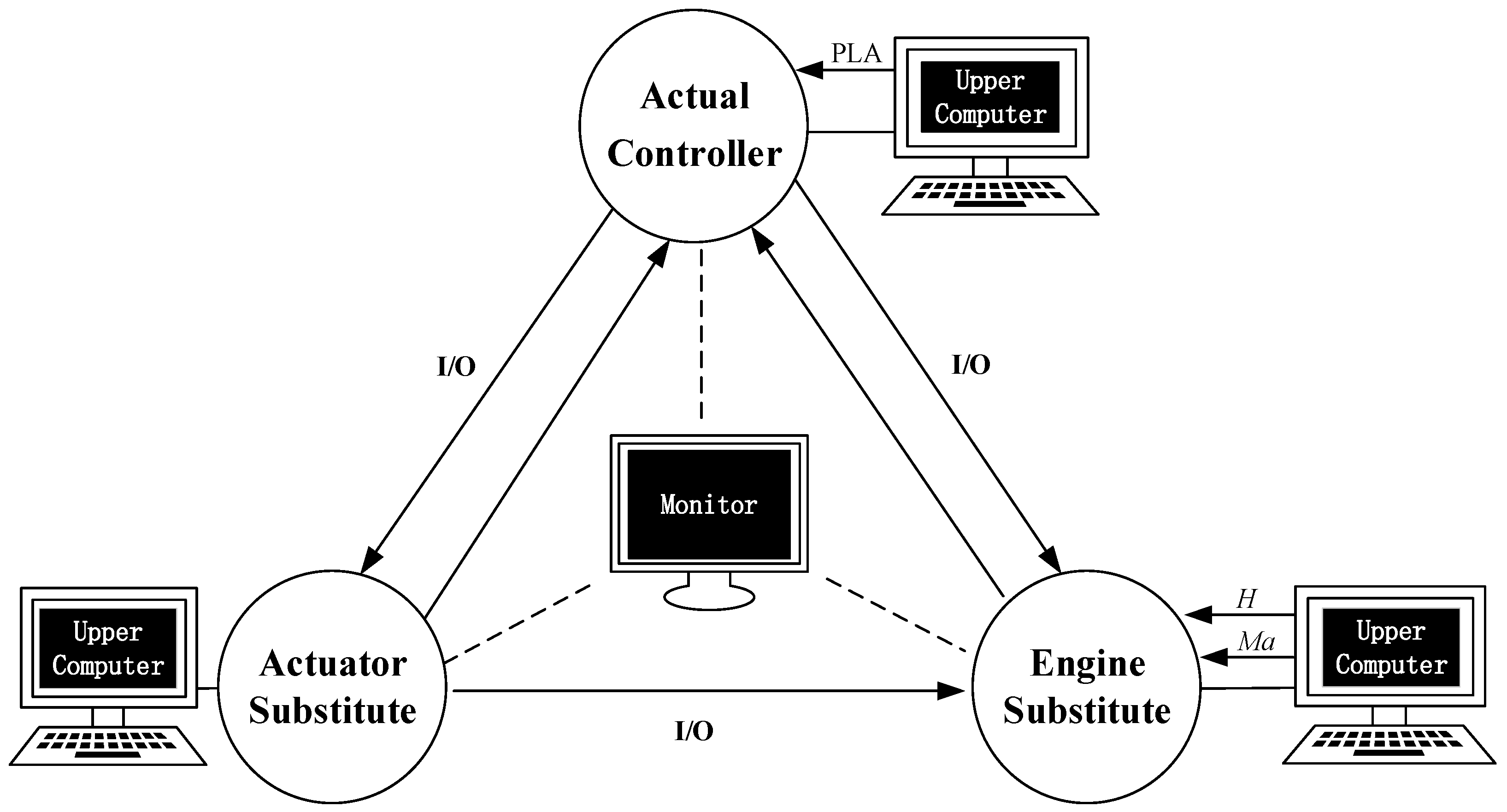
The configuration of HIL is shown in Figure 11. The controller, equipped with the ADEMA and other necessary control programs, is the actual controller of the engine, except for the embedded controllers loaded with the models of the engine and actuator, which serve as physical substitutes. Sensor and actuator faults are injected into the actual controller input/output, while other disturbances are injected into the controller to which the engine model belongs. The intake conditions of the engine are given by the upper computer, and the actual controller is in the laboratory’s normal temperature and pressure environment, except for receiving power lever angle (PLA) command sequences from the upper computer.
The controllers used for the actual controller, actuator substitute, and engine substitute are FT-M6678 DSP (Galaxy Flytech Processor, Tianjin, China), NI PXIe-1082 (National Instruments, Austin, TX, USA), and NI PXIe-8840 (National Instruments, Austin, TX, USA), respectively. The main frequency of FT-M6678 is 1.0 GHz; the rest are approximately 2.7 GHz. Using HIL to verify fault-tolerance within the flight envelope is a requirement of GJB10890-2023. This method can comprehensively verify the fault tolerance capability of the actual controller itself, since many faults are difficult to encounter in actual engine testing. ADEMA has an average running time of around 4 μs per control cycle (20 ms), with a maximum of no more than 40 μs.
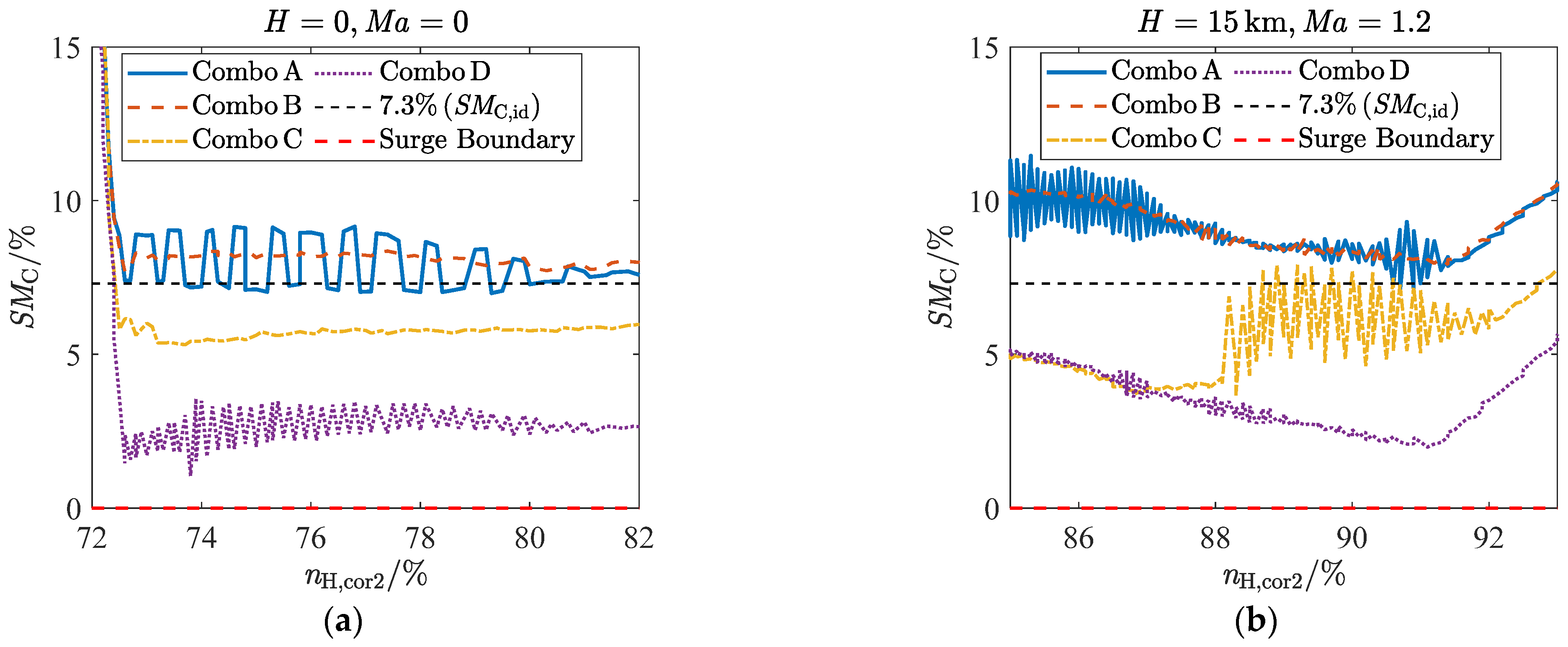
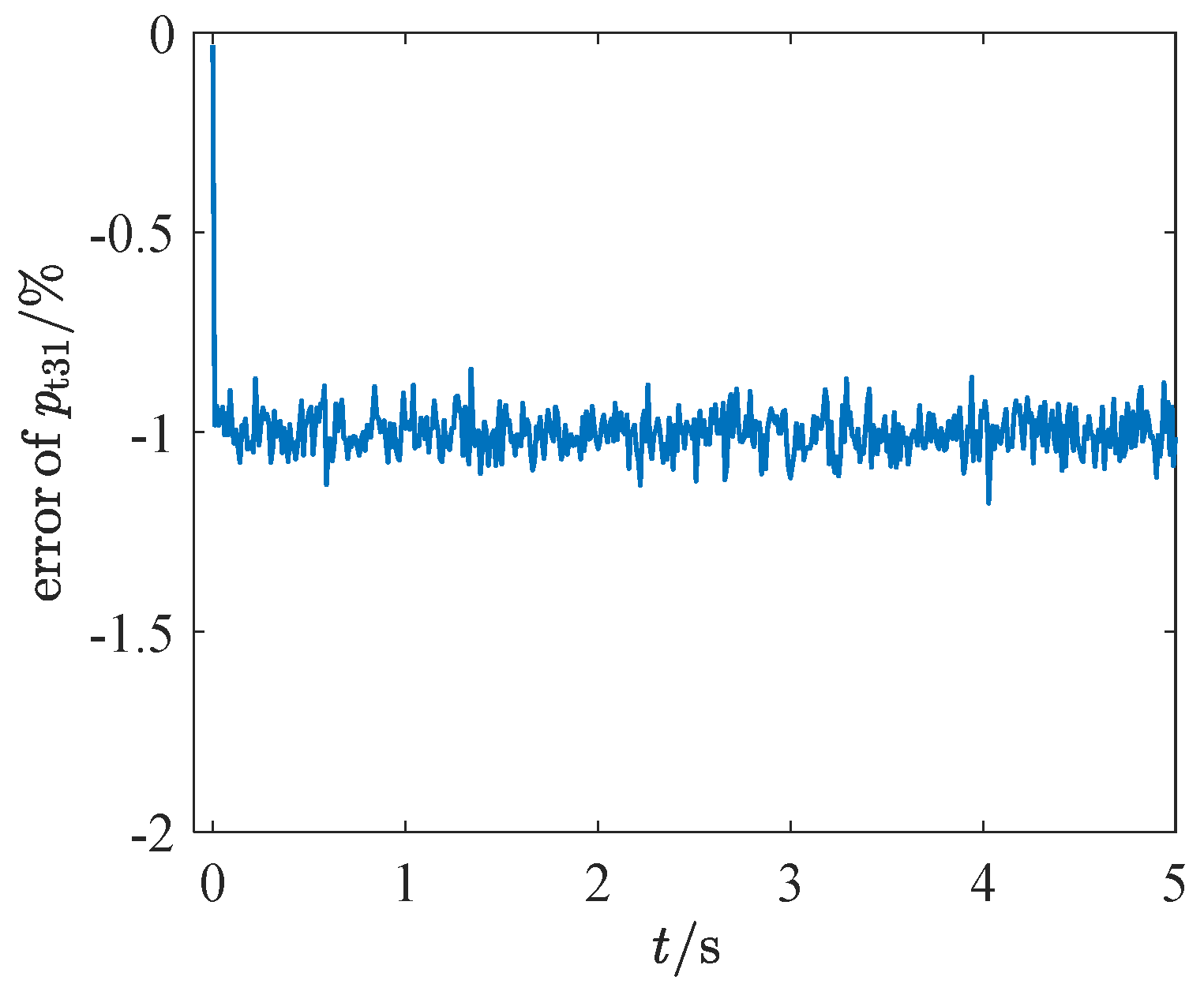
What we need to further verify is the combination of deviations or faults. The deviation or fault injection method described in Section 3, using the error of pt31 as an example, can be illustrated in Figure 12. This section provides the errors for the step signal part of the four disturbance combinations, as outlined in Table 3. Combo A represents the combination of normal deviations (including minor faults), Combo B represents the combination of a single significant fault and normal deviations from other factors, while Combo C and Combo D represent the combinations involving two significant faults and normal deviations from other factors.
Under four disturbance combinations, the effects of ADEMA in controlling the acceleration process at sea level (H = 0, Ma = 0) and an envelope point (H = 15 km, Ma = 1.2) based on the HIL are shown in Figure 13. It is evident that the ADEMA can effectively tolerate a single significant fault or minor faults while maintaining SMC near 7.3%. In the situations where two significant faults occur simultaneously, the ADEMA can still dilute the influence of Combo C at sea level, but the surge risk is greatly increased under Combo D. The inherent limitation of the four-redundancy configuration is that it cannot fully tolerate the impact of two significant faults.
Figure 13. The control effects of ADEMA in the HIL system under four disturbance combinations: (a) H = 0, Ma = 0; (b) H = 15 km, Ma = 1.2.
Aerospace 12 00829 g013

5.2. Sea Level Statistics

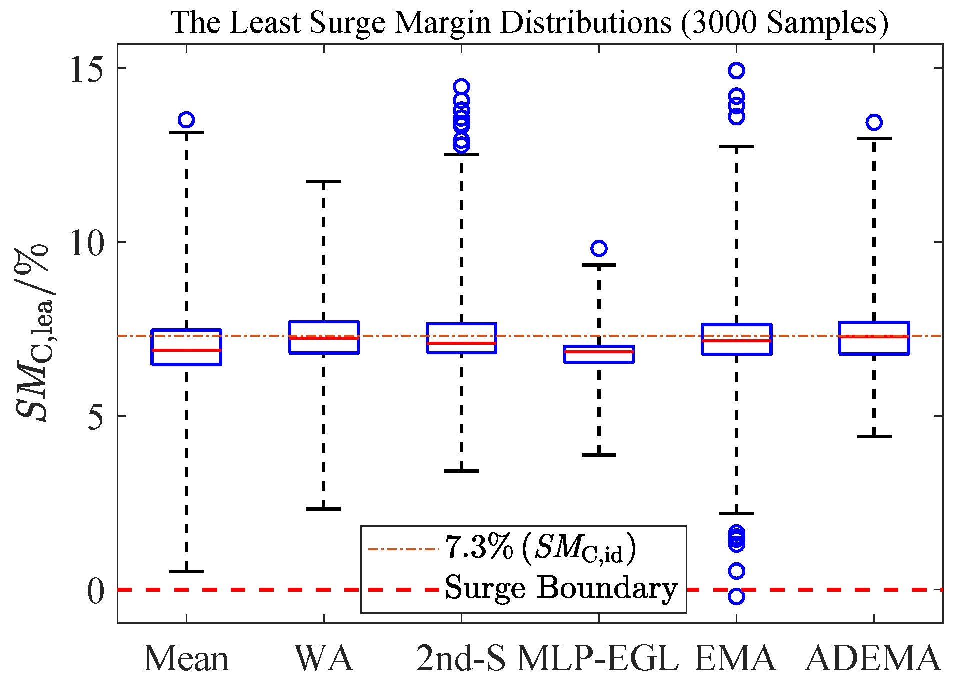
The statistical results under random disturbance combinations like Combo B are more convincing. Therefore, this section verifies the effectiveness of ADEMA by randomly injecting different disturbance combinations (a single significant fault and normal deviations from other factors) into 3000 sets of full acceleration processes and statistically analyzing the distribution of SMC,lea. The control result of Combo B in Figure 13a can be regarded as one of the 3000 sets. The SMC,lea statistical boxplots of different methods at sea level are presented in Figure 14. The “Mean” represents the mean of four fuels from four schedules as the output, embodying the idea of frequency school; the “WA” directly using P(z = i) (identical with the calculation method in Section 4) as the sample weight weighted average as a more prominent representative of the Bayesian school; the “2nd-S” signifies the second smallest fuel flow among fours, which is equivalent to the quantile; the “MLP-EGL” continues the strategy from the previous paper; the “EMA” is equivalent to the ADEMA when cA = 1. The essential difference between ADEMA and WA is that it is not a weighted average of the samples, but a weighted average of the corresponding distributions of the samples. Compared to the classical Kalman filter in the previous paper, WA avoids updating weights during each control cycle of the acceleration process, making it more adaptable to the effects of large-scale disturbances. Our method comparison ensures identical test conditions (same envelope points, same fault magnitudes and so on). It is evident that the methods based on symmetric distribution assumptions (EMA and Mean) struggle to adapt to impacts involving single significant faults.
The main statistical indices of SMC,lea of different methods at sea level are presented in Table 4. For a sample size of 3000, the 95% confidence interval of a statistic is approximately ±1.79%. While numerous indices are essential for a comprehensive statistical analysis, the evaluation of fault-tolerant acceleration control primarily focuses on three key aspects: 1. Minimum surge margin; 2. Overall standard deviation; 3. Accuracy of estimation. Using the median for accuracy evaluation offers greater stability compared to the sample mean and mode. Following this criterion, ADEMA exhibits the highest minimum SMC,lea (4.41%) and accuracy, with a standard deviation slightly higher than that of MLP-EGL. Even when assessed based on sample mean and mode, ADEMA still ranks second highest in accuracy. ADEMA reduces the median estimation error of MLP-EGL by 96%, showcasing remarkable advantages in ensuring security and accurate estimation, albeit with some trade-offs in concentration compared to the MLP-EGL. The WA method is only better than the EMA and the Mean. This indicates that ADEMA enables the engine to adopt a lower safety margin design under the same safety than WA method.
The distributions of acceleration times corresponding to these methods are depicted in Figure 15, where tacc represents the full acceleration time. It is typically required that tacc at sea level does not exceed 5 s under normal conditions. Even in the event of a significant fault, over 99% of tacc samples obtained through the fusion of the four schedules fall within the 5 s, as indicated in Table 5. However, while the maximum tacc for MLP-EGL stands at only 4.38 s, a small percentage (0.13%) of ADEMA samples exceed the 5 s reference. The 2nd-S method, on the other hand, is generally average in all aspects, exhibiting slightly lower minimum surge margin, higher standard deviation, lower accuracy, and an overall longer acceleration time when compared to ADEMA. The WA method has a slight advantage in maintaining stable acceleration time.

5.3. Flight Envelope Statistics

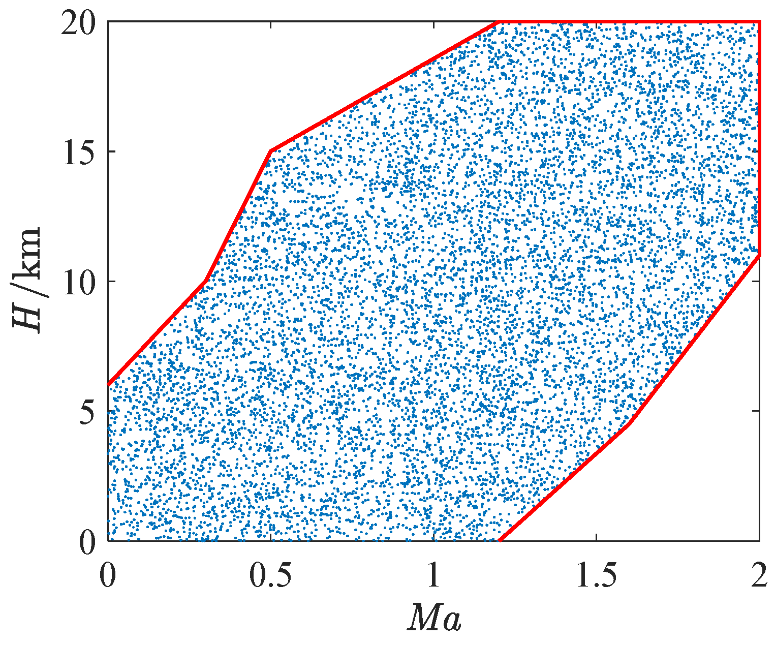
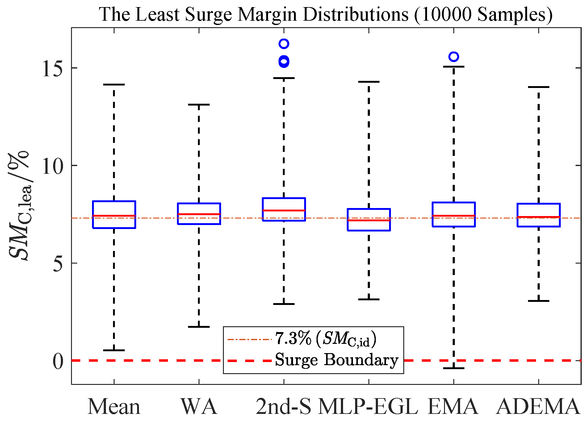
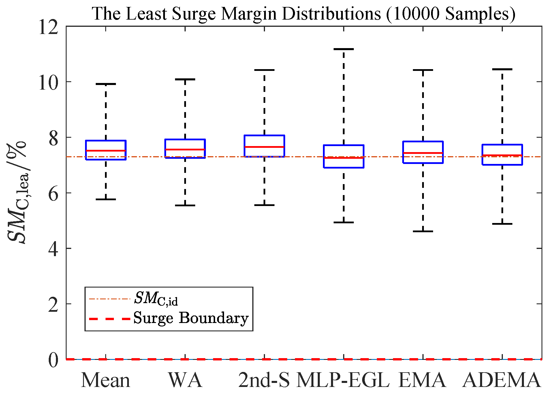
Similarly, the statistical distributions of SMC,lea, obtained by randomly sampling 10,000 points within the flight envelope (as illustrated in Figure 16 whose blue dots represent different intake conditions) and simultaneously injecting 10,000 disturbance combinations (which include a significant fault and other deviations), are shown in Figure 17. This study applies the envelope coverage principle—which defines a test envelope extending beyond the engine’s normal operating range—to validate the effects under diverse intake conditions. The main statistical indices of SMC,lea within the flight envelope are presented in Table 6. For a sample size of 10,000, the 95% confidence interval of a statistic is approximately ±0.98%. The Mean and EMA do not effectively prevent acceleration processes from approaching the surge boundary. The MLP-EGL achieves the highest minimum SMC,lea (3.14%) and the smallest standard deviation. The ADEMA demonstrates the highest accuracy, the second highest minimum SMC,lea and the second smallest standard deviation. ADEMA reduces the median estimation error of MLP-EGL by 36%. Within the full envelope, MLP-EGL exhibits the best performance, followed closely by ADEMA. From a security perspective, the WA method is slightly inferior to 2nd-S.
Table 6. The main statistics of SMC,lea of different methods within flight envelope under a significant fault and other deviations.
MeanWA2nd-SMLP-EGLEMAADEMA
Mode [%]7.317.367.457.137.287.21
Median [%]7.427.507.707.197.427.37
Mean [%]7.497.527.807.257.477.47
Absolute error of median [%]0.120.200.40−0.110.120.07
Relative error of median [%]1.642.745.481.511.640.96
Standard deviation [%]1.331.031.030.961.171.01
Minimum [%]0.531.732.903.14−0.393.06
Maximum [%]14.1413.1216.2414.2815.5714.01
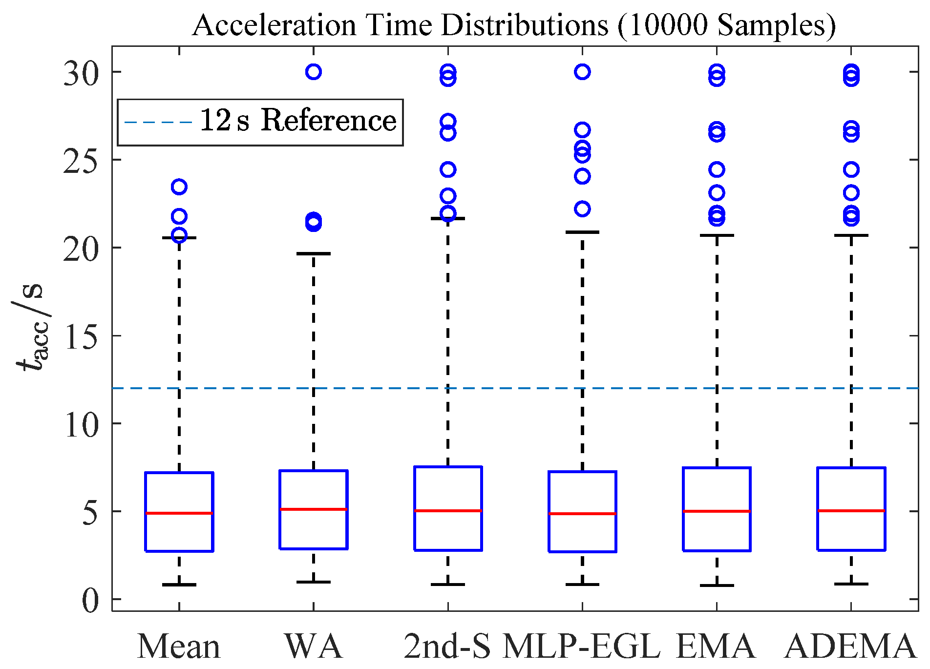
The tacc distributions of different methods within flight envelope are detailed in Figure 18, and the main statistics of tacc are presented in Table 7. Variations in flight intake air conditions significantly impact tacc, rendering the calculation of its maximum and minimum values less meaningful. Therefore, it is appropriate to consider samples exceeding 12 s as the primary benchmark for comparing tacc within the flight envelope. Following this criterion, the ranking of acceleration performance levels from high to low is as follows: Mean, MLP-EGL, ADEMA, EMA, and 2nd-S. Due to its limited security capabilities, the Mean method is not regarded as a reliable choice. Consequently, from a performance standpoint, MLP-EGL is favored over ADEMA, and the 2nd-S method ranks slightly below ADEMA across all indices. The WA method has a slight advantage in maintaining stable acceleration time.
The SMC, the statistical distributions within the flight envelope under the conditions of normal deviations (including minor faults) are shown in Figure 19, and the main statistical indices are provided in Table 8. The purpose of this verification is to reveal the difference between different probabilistic ideas. According to Equation (3), the Mean represents the expected value of minimum variance, which is referred to as “precision” in engineering. When a disturbance factor is significantly stronger than other factors, this advantage is overwhelmed. Notably, methods based on the modal idea (ADEMA, MLP-EGL, and EMA) consistently demonstrate high estimation accuracy under various disturbance conditions, which is termed “correctness” or “accuracy” in engineering. This implies that the idea of substantial probability does have the ability to capture essences. If the impact of a single significant fault is disregarded, the mean value is indeed a highly efficient choice; however, the boundary characteristics of acceleration control necessitate higher safety guarantees. Hence, the introduction of asymmetric distribution plays a crucial role in maintaining a safe distance from the surge boundary. The low standard deviation characteristic of MLP-EGL is not as stable as that of ADEMA here, indicating that its adaptive ability is inferior to that of the latter.

6. Conclusions

For the fault-tolerant problem of acceleration schedules in the turbofan, the relevant requirement necessitates the ability to withstand the impact of a single significant fault and normal deviations from other factors (including minor faults) without approaching the surge boundary significantly. This makes it difficult for methods based on traditional probability ideas and symmetric distributions to meet the requirements, whereas the substantial probability idea identified in this study is well-suited for adjusting the distribution structure of estimates—enhancing the possibility of maintaining a safe distance from the surge boundary while ensuring estimation accuracy. The known parameters required for ADEMA are only the real-time fuel flow rates obtained from the four acceleration schedule outputs at each moment, as well as their past cumulative variances (vi). Except for a few basic parameters that require experience to set, no data is needed to adjust key parameters. This represents the most significant engineering advantage over supervised learning methods like MLP-EGL. In the subsequent verifications, the SMC,lea and tacc distributions of the Mean, WA, 2nd-S, MLP-EGL, EMA and ADEMA methods were compared under various random disturbance combinations involving a single significant fault and other deviations:
  • During operation test under simple fault conditions, it was shown that the ADEMA based on a four-redundancy configuration can better withstand the effects of a single significant fault and other normal deviations (including minor faults), but cannot completely block the effects of two significant faults. Furthermore, the fault-tolerant capability of the acceleration schedules makes low margin design possible, that is, a 7.3% SMC,id can decrease acceleration time by 16.5% compared to a 12% SMC,id;
  • In the context of sea level statistics, ADEMA exhibits the highest minimum SMC,lea and accuracy, with its standard deviation only slightly exceeding that of MLP-EGL. ADEMA reduces the median estimation error of MLP-EGL by 96%;
  • In the context of flight envelope statistics, ADEMA showcases the highest accuracy, the second highest minimum SMC,lea and the second smallest standard deviation. ADEMA decreases the median estimation error of MLP-EGL by 36%.
  • While both frequentist and Bayesian frameworks center their optimization on variance reduction, substantial probability shifts the emphasis to the accuracy in a narrow sense.
A major contribution of this paper is demonstrating how MLP-EGL and ADEMA both conform to the proposed substantial probability paradigm. In engineering practice, ADEMA may become a default option unless high-fidelity CLM-based fault data can be obtained. A key difference from MLP-EGL lies in this study’s transformation of the surge boundary’s unilateral constraint into an active skewing of the acceleration fuel flow distribution toward lower values, thereby incorporating the constraint implicitly rather than explicitly.
The lack of a formal central limit theorem for the mode makes theoretical proof of asymmetry’s constraining effect on estimation skewness impossible. Thus, some coefficients (like cA) are selected empirically. Numerical simulations show that reducing cA to 0.618 induces marked asymmetry in SMC,lea’s statistical results, and while further reduction continues to exacerbate asymmetry, the incremental effect diminishes toward zero. Thus, further theoretical investigation is needed to fully elucidate ADEMA’s impact on the skewness of mode estimation results. The method’s vulnerability to some dual-factor faults in turbofan acceleration applications is fundamentally limited by the quadruplex redundancy architecture’s capabilities. Future research should also address the following aspects:
(1) it is necessary to explore whether there exists a valid central limit law for modes, along with corresponding theoretical tools to support it, (2) and gradually advance this method to experiments of the micro turbojet to gain more universal support.

Author Contributions

Conceptualization, X.Z. and J.G.; methodology, X.Z.; software, X.Z.; validation, X.Z. and M.L.; formal analysis, K.W.; investigation, K.W.; resources, Z.S.; data curation, M.L.; writing—original draft preparation, X.Z.; writing—review and editing, J.G.; visualization, K.W.; supervision, J.G.; project administration, M.L.; funding acquisition, Z.S. All authors have read and agreed to the published version of the manuscript.

Funding

This research was supported by the National Key Research and Development Program of China, grant number 2022YFF0610903, National Major Science and Technology Projects of China, grant number T01 project, and the Article Processing Charge was funded by Xi’an Jiaotong University.

Data Availability Statement

The data presented in this study are available on request from the corresponding author due to certain confidentiality obligations.

Conflicts of Interest

The authors declare no conflicts of interest.

Abbreviations

The following abbreviations are used in this manuscript:
ADEMAAsymmetric Distribution Expectation-Maximum Algorithm
CLMComponent Level Model
EMAExpectation-Maximum Algorithm
HILHardware-In-the-Loop
HPCHigh-Pressure Compressor
HPTHigh-Pressure Turbine
LPTLow-Pressure Turbine
MLP-EGLMulti-Layer Perceptron with Exponential Gumbel Loss
N-dotSpeed Derivative
WAWeighted Average
2nd-Sthe 2nd Smallest value

References

  1. Jaw, L.C.; Mattingly, J.D. Aircraft Engine Controls: Design, System Analysis, and Health Monitoring; American Institute of Aeronautics and Astronautics: Reston, VA, USA, 2009; pp. 119–124. [Google Scholar]
  2. Walsh, P.P.; Fletcher, P. Gas Turbine Performance; Blackwell Science: Hoboken, NJ, USA, 2004; pp. 459–464. [Google Scholar]
  3. Wang, J.; Zhang, W.; Hu, Z. Model-Based Nonlinear Control of Aeroengines; Springer Singapore Pte. Limited: Singapore, 2021; pp. 185–194. [Google Scholar]
  4. Connolly, J.W.; Csank, J.; Chicatelli, A. Advanced Control Considerations for Turbofan Engine Design. In Proceedings of the 52nd AIAA/SAE/ASEE Joint Propulsion Conference, Salt Lake City, UT, USA, 25–27 July 2016. [Google Scholar]
  5. Wei, Z.; Zhang, S. Auto-updating model-based control for thrust variation mitigation and acceleration performance enhancement of gas turbine aero-engines. Propuls. Power Res. 2023, 13, 394–415. [Google Scholar] [CrossRef]
  6. MYERS, L.; Burcham, F.W., Jr. Preliminary flight test results of the F100 EMD engine in an F-15 airplane. In Proceedings of the 20th Joint Propulsion Conference, Cincinnati, OH, USA, 11–13 June 1984. [Google Scholar]
  7. Dubrova, E. Fault-Tolerant Design; Springer: New York, NY, USA, 2013; pp. 12–17. [Google Scholar]
  8. Gu, Z.; Pang, S.; Li, Y.; Li, Q.; Zhang, Y. Turbo-fan engine acceleration control schedule optimization based on DNN-LPV model. Aerosp. Sci. Technol. 2022, 128, 107797. [Google Scholar] [CrossRef]
  9. Wang, Y.; Fang, J.; Song, W.; Ji, C.; Zhang, H.; Zhao, Q. Surge-Elimination Strategy for Aero-Engine Transient Control. J. Dyn. Syst. Meas. Control. 2024, 146, 041007. [Google Scholar] [CrossRef]
  10. Wang, K.; Xu, M.; Li, M.; Geng, J.; Liu, J.; Song, Z. A multi-input based full envelope acceleration schedule design method for gas turbine engine based on multilayer perceptron network. Aerosp. Sci. Technol. 2022, 130, 107928. [Google Scholar] [CrossRef]
  11. Song, K.; Jia, L.; Chen, Y.; Tan, T. Design of acceleration control schedule for adaptive cycle engine based on direct simulation model. Chin. J. Aeronaut. 2024, 37, 307–318. [Google Scholar] [CrossRef]
  12. Khalid, S.J.; Diegelman, J. Improving Turbofan Transient Characteristics with Multiple Variable Geometry Closed Loop Control. In Proceedings of the AIAA Propulsion and Energy 2020 Forum, Virtual Event, 24–28 August 2020. [Google Scholar]
  13. Zhang, X.; Liu, J.; Li, M.; Geng, J.; Song, Z. Fusion Control of Two Kinds of Control Schedules in Aeroengine Acceleration Process. J. Propuls. Technol. 2022, 43, 344–357. [Google Scholar]
  14. Cai, C.; Zheng, Q.; Wang, Y.; Zhang, H.; Sun, F. Research on Optimal Control Method for Turbofan Engine Acceleration Process with Variable Air Bleed Considering High Pressure Turbine Guide Vane Life. Int. J. Aeronaut. Space 2023, 24, 475–487. [Google Scholar] [CrossRef]
  15. Wang, K.; Liao, Z.; Xu, M.; Li, M.; Duan, B.; Liu, J.; Song, Z. Robust acceleration schedule design for gas turbine engine using multilayer perceptron network with adaptive sample class weighting. Aerosp. Sci. Technol. 2024, 154, 109500. [Google Scholar] [CrossRef]
  16. Zhang, X.; Wang, K.; Geng, J.; Li, M.; Song, Z. A fault-tolerant acceleration control strategy for turbofan engine based on multi-layer perceptron with exponential Gumbel loss. Energy 2024, 294, 130873. [Google Scholar] [CrossRef]
  17. Mohammadi, E.; Montazeri-Gh, M. Active Fault Tolerant Control with self-enrichment capability for gas turbine engines. Aerosp. Sci. Technol. 2016, 56, 70–89. [Google Scholar] [CrossRef]
  18. Liu, L.; Liu, T.; Chen, C.L.P.; Wang, Y. Modal-Regression-Based Broad Learning System for Robust Regression and Classification. IEEE Trans. Neur. Net. Lear. 2024, 35, 12344–12357. [Google Scholar] [CrossRef] [PubMed]
  19. Yao, W.; Lindsay, B.G.; Li, R. Local modal regression. J. Nonparametric Stat. 2012, 24, 647–663. [Google Scholar] [CrossRef]
  20. Yao, W.; Li, L. A New Regression Model: Modal Linear Regression. Scand. J. Stat. 2014, 41, 656–671. [Google Scholar] [CrossRef]
  21. Feng, Y.; Fan, J.; Suykens, J.A.K. A Statistical Learning Approach to Modal Regression. J. Mach. Learn. Res. 2020, 21, 1–35. [Google Scholar]
  22. Wang, K.; Li, S. Robust distributed modal regression for massive data. Comput. Stat. Data Anal. 2021, 160, 107225. [Google Scholar] [CrossRef]
  23. Liu, Q.; Huang, X.; Bai, R. Bayesian modal regression based on mixture distributions. Comput. Stat. Data Anal. 2024, 199, 108012. [Google Scholar] [CrossRef]
  24. Li, L.; Yuan, Y.; Zhang, X.; Wu, S.; Zhang, T. Fault-Tolerant Control Scheme for the Sensor Fault in the Acceleration Process of Variable Cycle Engine. Appl. Sci. 2022, 12, 2085. [Google Scholar] [CrossRef]
  25. Qiu, X.; Chang, X.; Chen, J.; Fan, B. Research on the Analytical Redundancy Method for the Control System of Variable Cycle Engine. Sustainability 2022, 14, 5905. [Google Scholar] [CrossRef]
  26. Zhou, J.; Liu, Y.; Zhang, T. Analytical Redundancy Design for Aeroengine Sensor Fault Diagnostics Based on SROS-ELM. Math. Probl. Eng. 2016, 2016, 8153282. [Google Scholar] [CrossRef]
  27. Zhang, Z.; Huang, X.; Zhang, T. Analytical Redundancy of Variable Cycle Engine Based on Proper Net considering Multiple Input Variables and the Whole Engine’s Degradation. Int. J. Aerosp. Eng. 2021, 2021, 9959264. [Google Scholar] [CrossRef]
  28. Ma, Y.; Du, X.; Sun, X.; Zhao, F. Active fault tolerant tracking control of turbofan engine based on virtual actuator. ISA Trans. 2022, 122, 247–259. [Google Scholar] [CrossRef] [PubMed]
  29. Cheng, D.; Liu, L.; Yu, Z. CNN-Based Intelligent Fault-Tolerant Control Design for Turbofan Engines with Actuator Faults. IEEE Access 2021, 9, 28122–28139. [Google Scholar] [CrossRef]
  30. Ring, D.; Christiansson, A.; Härefors, M. Fault Tolerant Multivariable Control of a Military Turbofan Engine. In Proceedings of the 16th Triennial World Congress, Lisbon, Portugal, 21–24 May 2005. [Google Scholar]
  31. Peng, K.; Zhang, Z.; Yang, F.; Jiao, C. Active Fault-tolerant Control of Auxiliary Power Unit Based on Analytical Redundancy and Heterogeneous Redundancy Design. In Proceedings of the 2019 IEEE 10th International Conference on Mechanical and Aerospace Engineering, Brussels, Belgium, 22–25 July 2019. [Google Scholar]
  32. GJB10890-2023; General Specification for Digital Control System of Aircraft Engines. Army GADO: Beijing, China, 2023.
  33. Ren, C.; Sun, D.; Dey, D.K. Bayesian and frequentist estimation and prediction for exponential distributions. J. Stat. Plan. Infer. 2006, 136, 2873–2897. [Google Scholar] [CrossRef]
  34. Silverman, B.W. Density Estimation for Statistics and Data Analysis; Taylor & Francis Group: Oxfordshire, UK, 1998. [Google Scholar]
  35. Qiu, X. Neural Networks and Deep Learning; China Machine Press: Beijing, China, 2019. [Google Scholar]
  36. Liu, Z.; Liu, Y.; Yu, Y.; Yang, R. Advanced fuel limit design to improve dynamic performance of marine three-shaft gas turbine. Appl. Therm. Eng. 2024, 236, 121649. [Google Scholar] [CrossRef]
  37. ISO 2314:2009(E); Gas Turbines-Acceptance Tests. ISO: Geneva, Switzerland, 2009.
  38. Zhao, H.; Liao, Z.; Liu, J.; Li, M.; Liu, W.; Wang, L.; Song, Z. A highly robust thrust estimation method with dissimilar redundancy framework for gas turbine engine. Energy 2022, 245, 123255. [Google Scholar] [CrossRef]
  39. Liao, Z.; Wang, J.; Liu, J.; Geng, J.; Li, M.; Chen, X.; Song, Z. Uncertainties in gas-path diagnosis of gas turbines: Representation and impact analysis. Aerosp. Sci. Technol. 2021, 113, 106724. [Google Scholar] [CrossRef]
  40. Xu, M.; Liu, J.; Li, M.; Geng, J.; Wu, Y.; Song, Z. Improved hybrid modeling method with input and output self-tuning for gas turbine engine. Energy 2022, 238, 121672. [Google Scholar] [CrossRef]
  41. Xu, M.; Wang, J.; Liu, J.; Li, M.; Geng, J.; Wu, Y.; Song, Z. An improved hybrid modeling method based on extreme learning machine for gas turbine engine. Aerosp. Sci. Technol. 2020, 107, 106333. [Google Scholar] [CrossRef]
  42. Song, K.; Jia, L.; Chen, Y.; Tan, T.; Fan, P. Optimization of ACE mode transition control schedule considering geometric adjustment speed. Int. J. Turbo Jet Eng. 2024, 40 (Suppl. 1), s389–s398. [Google Scholar] [CrossRef]
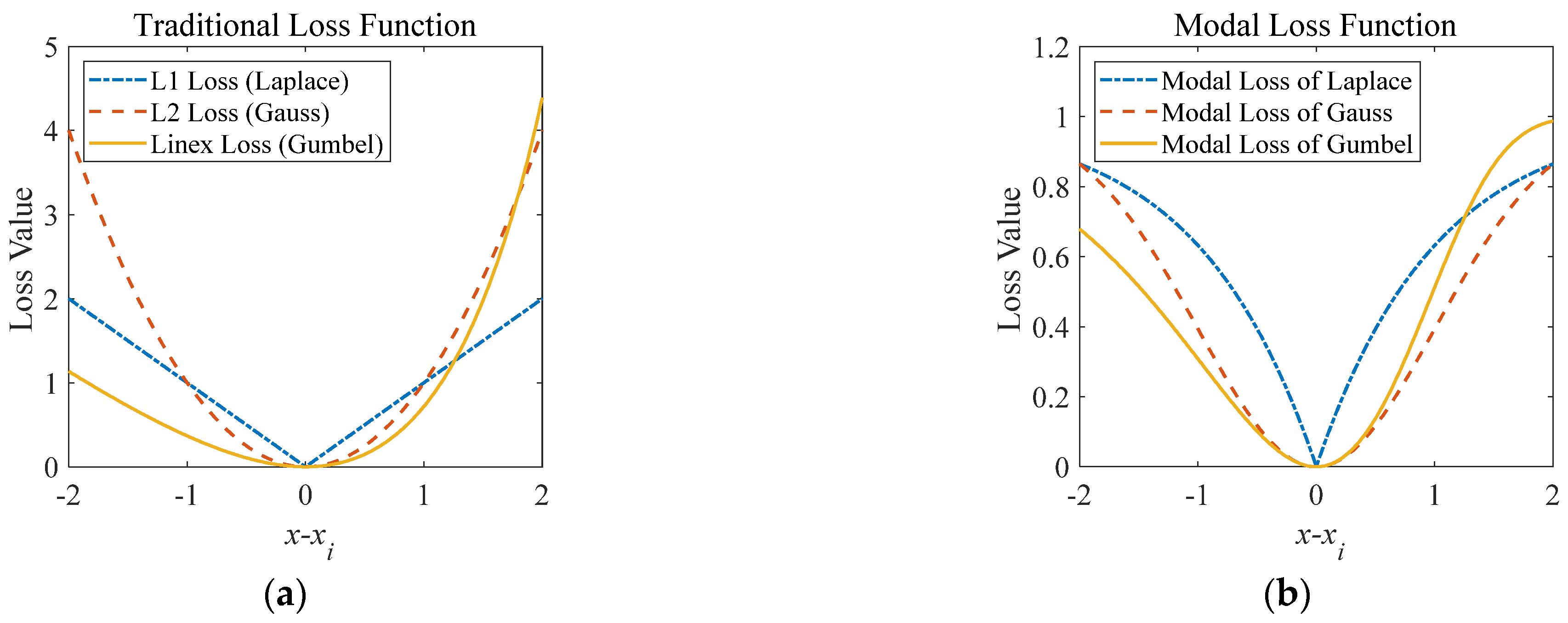
Figure 1. The loss function comparison: (a) Traditional loss functions; (b) Modal loss functions.
Aerospace 12 00829 g001
Figure 2. The density estimation with Gaussian kernel.
Aerospace 12 00829 g002
Figure 3. Stage definitions of the hybrid exhaust turbofan.
Aerospace 12 00829 g003
Figure 4. Characteristic map of the HPC.
Aerospace 12 00829 g004
Figure 5. The main fuel control of the turbofan above idle state.
Aerospace 12 00829 g005
Figure 6. The control diagram of ADEMA for four acceleration schedules.
Aerospace 12 00829 g006
Figure 7. The asymmetric Gaussian distribution.
Aerospace 12 00829 g007
Figure 9. Acceleration control results at sea level of SMC,id = 7.3% and SMC,id = 12%: (a) Thrust versus t; (b) SMC versus nH,cor2.
Aerospace 12 00829 g009
Figure 10. The control effects of ADEMA in the HIL system under a significant fault: (a) H = 0, Ma = 0; (b) H = 11 km, Ma = 0.9.
Aerospace 12 00829 g010
Figure 11. The configuration of HIL.
Aerospace 12 00829 g011
Figure 12. The minor fault signal for the error of pt31.
Aerospace 12 00829 g012
Figure 14. The SMC,lea boxplots of different methods at sea level under a significant fault and other deviations.
Aerospace 12 00829 g014
Figure 15. The tacc boxplots of different methods at sea level under a significant fault and other deviations.
Aerospace 12 00829 g015
Figure 16. The envelope points and flight envelope.
Aerospace 12 00829 g016
Figure 17. The SMC,lea boxplots of different methods within flight envelope under a significant fault and other deviations.
Aerospace 12 00829 g017
Figure 18. The tacc boxplots of different methods within the flight envelope under a significant fault and other deviations.
Aerospace 12 00829 g018
Figure 19. The SMC,lea boxplots of different methods within the flight envelope in case of normal deviations.
Aerospace 12 00829 g019
Table 1. The accuracy of the main measurement types.
Measurement TypeNormal AccuracyDegraded Accuracy
Pressure±0.3%±0.5%
Temperature±0.15%±0.2%
Fuel flow±0.65%±1.0%
Table 3. The step signal error set of the disturbance combinations.
Disturbance FactorCombo ACombo BCombo CCombo D
Lex100 kW∙(nH,Cor2)2100 kW∙(nH,Cor2)2100 kW∙(nH,Cor2)2100 kW∙(nH,Cor2)2 + 200 kW
pt2 sensor−0.1%−0.1%−10%−0.1%
pt25 sensor0.5%0.5%0.5%0.5%
pt31 sensor−1%−10%−1%−1%
Wf metering−1.5%−1.5%15%15%
Tt2 sensor−0.2%−0.2%−0.2%−0.2%
Tt25 sensor0.2%0.2%0.2%0.2%
ΔSEC0000
ΔSWC0000
ΔSEHT0000
ΔSWHT0000
Table 4. The main statistics of SMC,lea of different methods at sea level under a significant fault and other deviations.
MeanWA2nd-SMLP-EGLEMAADEMA
Mode [%]6.866.916.866.877.277.46
Median [%]6.887.237.096.847.167.28
Mean [%]6.967.257.316.787.147.27
Absolute error of median [%]−0.42−0.07−0.21−0.46−0.14−0.02
Relative error of median [%]−5.75−0.96−2.88−6.30−1.92−0.27
Standard deviation [%]1.230.970.920.661.000.82
Minimum [%]0.532.313.413.87−0.204.41
Maximum [%]13.5111.7414.469.8114.9313.44
Table 5. The main statistics of tacc of different methods at sea level under a significant fault and other deviations.
MeanWA2nd-SMLP-EGLEMAADEMA
Median [s]3.743.723.763.723.743.74
Standard deviation [s]0.200.170.190.130.190.18
Proportion of tacc > 5 s [%]000.2000.170.13
Minimum [s]3.083.143.203.243.003.32
Maximum [s]4.964.725.484.385.605.56
Table 7. The main statistics of tacc of different methods within the flight envelope under a significant fault and other deviations.
MeanWA2nd-SMLP-EGLEMAADEMA
Median [s]4.905.105.044.855.005.02
Standard deviation [s]3.223.103.413.333.413.39
Proportion of tacc > 12 s [%]3.943.485.004.354.974.91
Table 8. The main statistics of SMC,lea of different methods within the flight envelope in case of normal deviations.
MeanWA2nd-SMLP-EGLEMAADEMA
Mode [%]7.467.427.527.107.367.30
Median [%]7.527.567.657.267.437.35
Mean [%]7.577.617.707.367.477.39
Absolute error of median [%]0.220.260.35−0.040.130.05
Relative error of median [%]3.013.604.790.551.780.68
Standard deviation [%]0.540.530.590.710.660.62
Minimum [%]5.765.545.554.944.614.88
Maximum [%]9.9210.0810.4211.1710.4210.44
Disclaimer/Publisher’s Note: The statements, opinions and data contained in all publications are solely those of the individual author(s) and contributor(s) and not of MDPI and/or the editor(s). MDPI and/or the editor(s) disclaim responsibility for any injury to people or property resulting from any ideas, methods, instructions or products referred to in the content.