Ensemble Modeling Method for Aero-Engines Based on Automatic Neural Network Architecture Search Under Sparse Data

Abstract

In this paper, the problem of aero-engines ensemble modeling under sparse data is addressed. Firstly, the Makima method is used to interpolate and complement the sparse data by analyzing the experimental data of a specific real aero-engine. In this way, the data sparsity problem due to sampling or transmission is solved equally well. Secondly, the Nonlinear Auto-Regressive with Exogenous Inputs (NARX) neural network is brought in as the computational structure of the model. Based on the Automatic Neural Network Architecture Search (ANAS) method, the hyperparameters of the model can be searched efficiently, and the performance is improved. Third, a novel ensemble modeling method based on the Makima method, the NARX model, and the ANAS method is proposed to realize high-precision modeling throughout the entire operation process of the aero-engine from the idle state to the full throttle state. Finally, the proposed method is validated by simulations and experiments, and the results illustrate the innovation and correctness.

1. Introduction

The structure of an aero-engine is complex, and its response characteristics are affected by various factors such as intake conditions, flight status, and load variations, rendering it a typical system characterized by strong coupling, fast time-varying, nonlinearity, and uncertainty. Modeling such a system with large-scale and high precision within the flight envelope presents significant challenges [1,2,3]. Additionally, data are often sparse and incomplete due to physical limitations or faults of the data sampling system, external disturbances, and packet loss during transmission in practical operations. This sparsity caused by data loss further increases the difficulty of modeling [4,5]. However, effective modeling technology is essential for precise monitoring, fault diagnosis, control optimization, and performance prediction of aero-engines [6,7,8,9]. Therefore, conducting relevant research to address the special challenges in the aero-engine modeling methods has fundamental significance. An increasing number of researchers have focused on consensus protocols with specific convergence requirements.

Researchers have conducted a considerable amount of work in this field. Existing studies can generally be categorized into three types: “white- box” model, “gray- box” model, and “black- box” model. The basic principle of the “white- box” model involves establishing a gas turbine mathematical model based on the Brayton cycle principles. This is achieved by solving three types of nonlinear equilibrium equations: flow continuity equations, pressure balance equations, and power balance equations, according to the work characteristics of each component. Noteworthy works in this domain include [10,11,12]. The primary challenges of the white-box model include (1) model convergence issues, real-time performance concerns arising from multiple iterative computations, and precision dependency of model accuracy on component characteristics; (2) degradation in engine component performance or actual installation errors can easily lead to model mismatch; and (3) models obtained through this method are challenging to apply in control design directly. The “gray-box” model often employs a data- and model-collaborative-driven architecture, where the model structure is derived based on the mechanistic approach [13,14,15], and the specific parameters of the architecture are identified through data-driven methods. This approach combines the advantages of both white-box and black-box models. In [16], a jet propulsion engine model was derived using a sparse identification method, and both batch least squares and recursive extended Kalman Filter were utilized for “gray-box” estimation. Wei et al. [17] presented an onboard modeling method for gas turbine aero-engines based on a Hybrid Wiener Model (HWM) that utilized engine monitoring data. However, similar to the white box model, the mechanistic approach demands a considerable level of professional technical expertise from researchers, and the inaccuracy of component characteristics obtained by data-driven methods will seriously affect the model’s accuracy.

To tackle the challenges mentioned above, researchers have developed “black-box” models, with typical instances encompassing fuzzy system models [18,19,20,21] and artificial neural network models [22,23], among others. Although these models have demonstrated excellent performance in applications of aero-engines, especially when dealing with intricate nonlinear and time-varying characteristics, past applications have been restricted by constraints imposed by hardware and software systems. Recent technological advancements have significantly enhanced the data acquisition, computing, storage, and communication capabilities of aero-engine control systems, providing a solid foundation for new methods. In particular, innovations in artificial intelligence and Big Data offer fresh perspectives for developing “black-box” model [24,25,26]. In [27,28], the data-driven “black-box” model is proposed, which does not depend on the physical mechanisms or fundamental equations of the system but learns the behavior of the system through input-output data. For example, Study [29] proposes a framework combining Autoencoders and Gaussian Mixture Models (GMMs). It focuses on fault early warning in unsupervised scenarios. Study [30] presents a comprehensive and valuable comparison of advanced modeling techniques, including Autoencoders, LSTMs, and Gaussian processes, for predictive maintenance. This work provides significant insights into uncertainty quantification, successfully demonstrating the capabilities of complex deep learning architectures. Another study [31] offers a innovative approach by integrating Automated Feature Engineering (AFE) with Artificial Neural Networks to significantly improve the reliability of health status predictions. This method effectively addresses feature selection challenges and enhances model performance. The primary objective of the frameworks in [29,30,31] is to achieve accurate predictions over long horizons. In comparison, control applications have different needs, placing with a particular emphasis on model interpretability, minimal latency, and the ability to precisely capture transient dynamics for immediate feedback.

The NARX model structure is derived from dynamic system theory, making it more suitable for formulating control-oriented models that must interact with a controller in real-time, as required in our study. De Giorgi and Quarta [22] developed and validated a hybrid method combining the multigene genetic programming (GP) algorithm with artificial neural networks based on the NARX model, utilizing real flight data to simulate the transient behavior of the Viper 632-43 military turbojet engine, achieving promising results. In [23], a method in which two NARX models collaborate was proposed for predicting the specific fuel consumption of a turboshaft engine during instantaneous flight maneuvers, which demonstrates its adaptability to “sudden operating condition changes”. Xu et al. [32] introduced a digital twin model (DTM) based on NARX, which can accurately predict engine gas path parameters, and further verifies the reliability of NARX in predicting core performance parameters.The above works demonstrate that modeling engines using the NARX model is feasible and yields good results. Therefore, we adopt a data-driven NARX “black- box” model to construct a high-precision model of the entire operation process of a specific aero-engine in this paper.

However, existing “black- box” modeling methods face two main issues: (1) Due to physical limitations of the data sampling system, system faults, or data packet loss during transmission, the data are often sparse and incomplete. This missing data leads to sparsity, which reduces model accuracy and prevents effective generalization, sometimes even causing the model to fail to converge [33,34,35]. (2) Although the NARX model theoretically has the potential to achieve a high-performance model, the actual performance is often highly sensitive to hyperparameters. Traditional approaches typically involve manual tuning of hyperparameters, such as the number of neurons in the hidden layers, transfer functions, delay orders, training functions, and output layer transfer functions. These methods are inefficient and do not guarantee optimal results, lacking theoretical or experimental guidelines, making it difficult to obtain a convergent NARX model [36,37,38]. To address the above issues, we propose an ANAS-based ensemble modeling method for aero-engines using sparse data, tackling the challenge of high-precision modeling throughout the entire engine operation range, from the idle state to the full throttle state. The main contributions of this paper are summarized as follows:

• To address issues of incomplete and poor-quality data caused by sensor faults, system limitations, external disturbances, and data packet loss, we employ the Makima method to interpolate and complete sparse data. Based on the local geometric structure and trend information of the data, this method constructs a highly smooth and reasonable interpolation function to generate new data containing information on the input-output mapping of the aero-engine, thereby effectively enhancing the continuity and completeness of the data. The dataset obtained through this method can reflect the actual operational states of the engine more comprehensively and accurately, effectively avoiding problems such as poor model accuracy and non-convergence caused by data sparsity.
• Based on actual operational data of the aero-engine and a new dataset obtained by the Makima method, we fully adopt the core principle of data-driven modeling and introduce a NARX neural network model. Considering the specificity of the data, we utilize an ANAS method to search for the hyperparameters [39,40]. In this way, we enhance the proposed method’s search efficiency and model accuracy.
• A novel ensemble modeling method for aero-engines is developed based on the Makima method, the NARX model, and the ANAS method. An experimental verification platform is designed, and the approach is validated through ground tests, achieving high-precision modeling of the entire operation process from the idle state to the full-throttle state. The results show that the aero-engine model obtained by the proposed ensemble modeling method demonstrates high performance in terms of convergence, accuracy, generalization ability, and real-time capability.

The subsequent sections of the paper are structured as follows: Section 2 provides a detailed description of the ensemble modeling problem for aero-engines under sparse data, along with relevant background knowledge. Section 3 presents the ensemble modeling method under sparse data, including modeling planning, the implementation of the NARX model, and the search process of the ANAS method. Section 4 involves simulations, experiments, and analysis, primarily delineating the experimental validation platform and methodology, followed by an analysis of the experimental results. Finally, some conclusions are given in Section 5.

2. Problem Formulation and Model Evaluation Indexes

The main objective of this paper is to find the following nonlinear mapping, which can be expressed as a difference equation as follows:

$$y_i\left(k\right)=f_i[u_i(k-1),u_i(k-2),\cdots ,u_i(k-n_{ui}),y_i(k-1),y_i(k-2),\cdots ,y_i(k-n_{yi})],$$

(1)

where $u_i$ is the input and $y_i$ is the output vector of the model, $n_{ui}$ and $n_{yi}$ are the delay orders of the input and output, respectively, which represent the order of the model. Specifically, for the experimental verification platform (a 100-kg thrust turbojet engine) in this paper, its input $u_1$ is the control parameter K value of the voltage to the oil pump motor, the output $y_1$ represents the aero-engine rotational speed $N_s$, and the output $y_2$ is the exhaust gas temperature $T_s$. According to the actual circuit design of the Engine Control Unit (ECU), the input voltage of the oil pump motor is determined by the following formula:

$$V_{\mathrm{pump}}=V_{\mathrm{Power}}·{\displaystyle \frac{K}{7500}},$$

(2)

where $V_{\mathrm{pump}}$ is the input voltage to the oil pump motor, and it positively correlates with the aero-engine’s steady-state fuel flow. $V_{\mathrm{power}}$ is the ECU supply voltage.

The NARX model, with its strong nonlinear mapping ability and autoregressive dynamic characteristics, is well-suited for representing the difference equations mentioned above. It is widely applied in time series modeling and forecasting [41,42,43,44], and is particularly effective for solving the modeling challenge presented in this paper. Therefore, the NARX model is employed to construct a comprehensive model of the entire operating process of an aero-engine. The evaluation indexes of the model adopt Average Absolute Relative Error (AARE) and Root Mean Squared Relative Error (RMSRE), which are calculated as follows:

$$AARE={\displaystyle \frac{1}{n}}\sum _{i=1}^n∥{\displaystyle \frac{y_i-{\widehat{y}}_i}{y_i}}∥,$$

(3)

$$RMSRE=\sqrt{{\displaystyle \frac{1}{n}}{\displaystyle \sum _{i=1}^n}{\left({\displaystyle \frac{y_i-{\widehat{y}}_i}{y_i}}\right)}^2},$$

(4)

where ${\widehat{y}}_i$ is the model estimate value, $y_i$ is the actual measurement value, and n is the number of samples.

In time series prediction and system modeling, the selection of the Average Absolute Relative Error (AARE) and Root Mean Square Relative Error (RMSRE) as evaluation indices—instead of common indices like MAE, RMSE, or MAPE—is based on the following scientific considerations:

• Scale Invariance: Unlike absolute error indexs (e.g., MAE, RMSE), AARE and RMSRE use relative errors (i.e., the ratio of error to the true value), making them insensitive to data scale variations. In engineering applications, data may span multiple orders of magnitude (e.g., variables with different dimensions like temperature, pressure, or flow). AARE and RMSRE enable fair evaluation of model performance across different magnitude data, avoiding evaluation biases caused by varying variable units.
• Differentiated Response to Extreme Errors: AARE calculates the mean of absolute relative errors, demonstrating robustness to outliers. It is suitable for scenarios where overall trend evaluation is more critical.RMSRE amplifies the impact of larger relative errors through squaring operations, imposing stricter penalties on significant deviations. This makes it ideal for fields requiring tight control of extreme prediction errors (e.g., fault warnings or safety-critical systems).
• Engineering Applicability: In dynamic system modeling (e.g., NARX), the relative magnitude of prediction errors is often more practically meaningful than absolute errors. For example, in process control, a 10 °C deviation might be catastrophic for a low-temperature reaction (e.g., 50 °C) but acceptable for a high-temperature reaction (e.g., 500 °C). AARE and RMSRE directly reflect the relative impact of errors, aligning more closely with the needs of engineering decision-making.

In summary, AARE and RMSRE are chosen for their scale robustness, sensitivity to critical errors, and engineering interpretability, making them particularly suitable for performance evaluation in multi-scale and nonlinear systems.

3. Ensemble Modeling Method Under Sparse Data

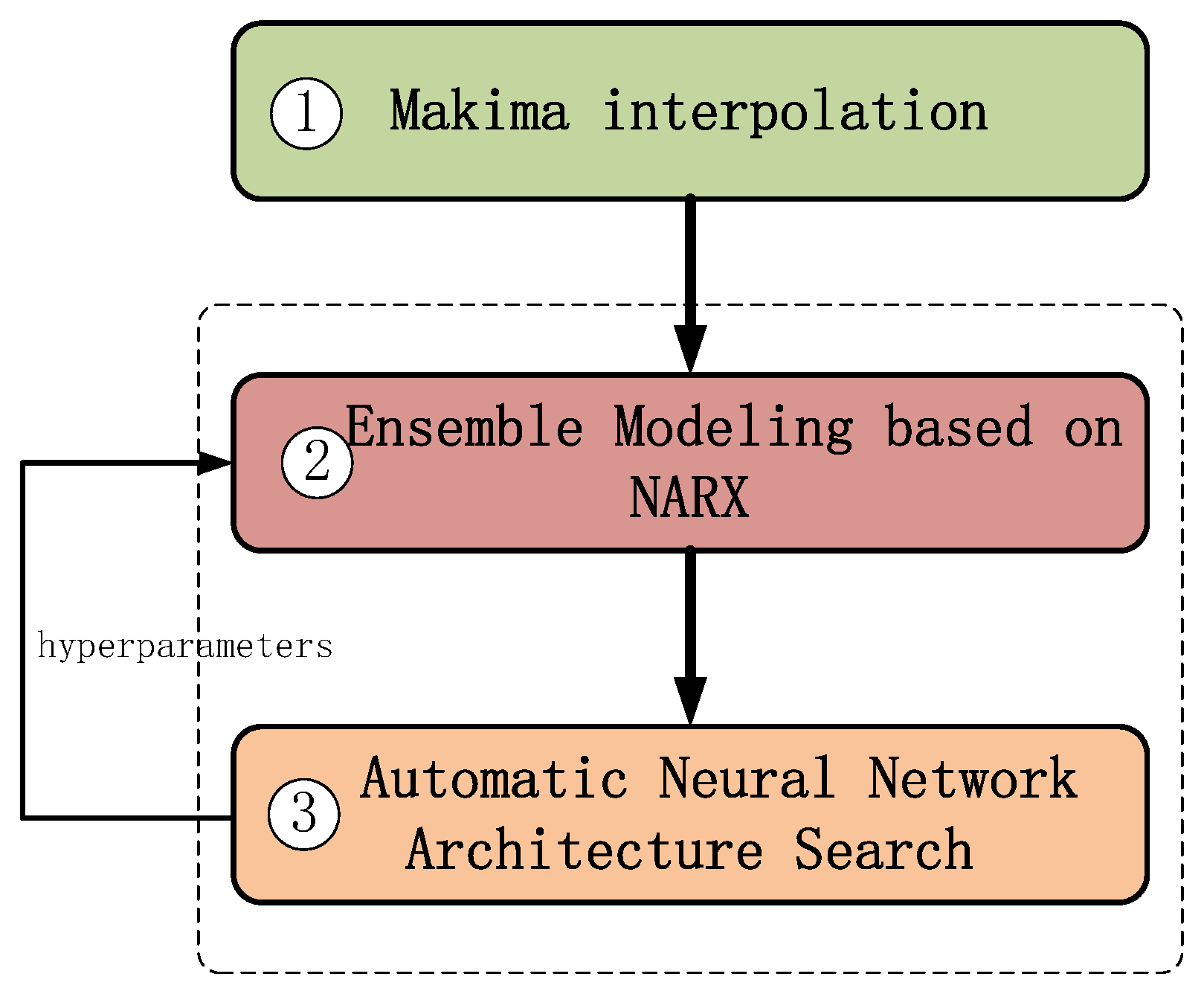
As shown in Figure 1, this section proposes three aspects: (1) Using the Makima interpolation method to solve the data sparsity problem. (2) Determining the overall framework and three work modes of the NARX model based on the ensemble modeling planning. (3) Adopting the method of Automatic Neural Network Architecture Search (ANAS), determining the hyperparameters of the network structure of the NARX model, which mainly includes the hidden layer neuron number, hidden layer transfer function type, input delay order, output delay order, training function type, and output layer transfer function type.

3.1. Makima Interpolation Method

Incomplete data and low data quality are common problems in aero-engine control systems. These problems are caused by situations such as sensor failures, physical limitations of the data sampling system, external disturbances, and data packet loss during transmission. To solve the data problem, this paper uses Makima interpolation to interpolate the sparse data for completeness according to the modeling requirements. Makima interpolation is a cubic Hermite interpolation method mainly used to smooth the estimation of function values between discrete data points. It approximates the original data by using cubic polynomials, thus providing smoother results than linear interpolation. Compared to spline interpolation, PCHIP, and cubic interpolation, this method is relatively simple to compute. The specific steps can be briefly described as follows [45,46]:

• Calculate slope: for each data point, calculate the slope of the two points before and after it.
• Modify the Akima algorithm: in order to avoid the case where the denominator is zero, Makima interpolation modifies the original Akima algorithm to ensure that the NaN result will not appear in the calculation process.
• Construct a cubic polynomial: using the calculated slope and curvature information, a cubic polynomial is constructed to approximate the function value between each data point. The specific algorithmic process can be referred to as the pseudo-code shown in Algorithm 1.

Algorithm 1 Work process of Makima interpolation method

Require:  $x=\left\{x\right[0],x[1],\dots ,x[n-1\left]\right\}$ // Known x-coordinates Require:  $y=\left\{y\right[0],y[1],\dots ,y[n-1\left]\right\}$ // Known y-coordinates Require:  num_points // Number of interpolation points Ensure:  $x_{\mathrm{interp}}=\{x_{\mathrm{interp}}\left[0\right],\dots ,x_{\mathrm{interp}}[\mathrm{num}\_\mathrm{point}-1]\}$ // Interpolated x-coordinates Ensure:  $y_{\mathrm{interp}}=\{y_{\mathrm{interp}}\left[0\right],\dots ,y_{\mathrm{interp}}[\mathrm{num}\_\mathrm{point}-1]\}$ // Interpolated y-coordinates  1: $n\leftarrow \mathrm{length}\left(x\right)$  2: for  $i\leftarrow 0$ to $n-2$ do  3:    $\mathrm{slopes}\left[i\right]\leftarrow {\displaystyle \frac{y[i+1]-y\left[i\right]}{x[i+1]-x\left[i\right]}}$ // Calculate slopes  4: end for  5: for $i\leftarrow 1$ to $n-2$ do  6:    $m\left[i\right]\leftarrow {\displaystyle \frac{\mathrm{slopes}[i-1]+\mathrm{slopes}\left[i\right]}{2}}$ // Average slopes for smoothness  7: end for  8: $m\left[0\right]\leftarrow \mathrm{slopes}\left[0\right]$ // Set boundary conditions  9: $m[n-1]\leftarrow \mathrm{slopes}[n-2]$ 10: for $j\leftarrow 0$ to $\mathrm{num}\_\mathrm{point}-1$ do 11:    $t\leftarrow {\displaystyle \frac{j}{\mathrm{num}\_\mathrm{point}-1}}$ // Normalized parameter 12:    $\mathrm{idx}\leftarrow \mathrm{floor}(t\times (n-\left(1\right))$ // Find corresponding interval 13:    $t\leftarrow (t\times (n-\left(1\right))-\mathrm{idx}$ // Compute local t in the interval 14:    $h\leftarrow x[\mathrm{idx}+1]-x\left[\mathrm{idx}\right]$ // Length of the interval 15:    $y_{\mathrm{interp}}\left[j\right]\leftarrow (1-t)·y\left[\mathrm{idx}\right]+t·y[\mathrm{idx}+1]+\{t·(1-t)$ 16:       $·\left({\displaystyle \frac{1}{3}}(m\left[\mathrm{idx}\right]·h+m[\mathrm{idx}+1]·h)-{\displaystyle \frac{1}{6}}{\displaystyle \frac{y[\mathrm{idx}+1]-y\left[\mathrm{idx}\right]}{h}}\right)\}$ 17:    $x_{\mathrm{interp}}\left[j\right]\leftarrow (1-t)·x\left[\mathrm{idx}\right]+t·x[\mathrm{idx}+1]$ 18: end for 19: return $(x_{\mathrm{interp}},y_{\mathrm{interp}})$

During the aero-engine test run, non-uniform and sparse test data often occur due to fluctuations in sampling frequency or data transmission packet loss. The Makima interpolation method demonstrates good adaptability to processing such data. Next, two cases are presented to compare the Makima interpolation method with the commonly used cubic Hermite interpolation method and cubic spline interpolation method, as shown in Figure 2.

• Case 1: Select the sampling points as (0, 0), (1, 0), (1.8, 0), (3,0.8), (3.9, 2), (5.2, 2), (6, 2).
• Case 2: The abscissa of the selected sampling point is x = [0, 0.6, 1, 1.5, 1.9, 2.5, 3.2, 3.6, 4.3, 4.6, 5], and the ordinate is obtained by function $y=1.5sin\left(2x\right)+cos\left(0.8x\right)$.

As shown in Figure 2, Makima effectively avoids the “overshoot” phenomenon and captures the movement between points well, demonstrating better performance than Hermite and cubic spline interpolation. Therefore, using the Makima method to address data sparsity is reliable.

Remark 1.

In this paper, we firstly assume that a large amount of data are lost randomly for some reason. The percentage of data lost in the worst-case scenario is as high as 80% of the total (the paper only takes the two cases of 80% and 50% loss as examples). We generated the missing data points using the Makima interpolation method described above and added them to the training dataset. Subsequent experimental validation shows that the model trained from the new dataset obtained by this method has a obvious performance improvement relative to the model trained from the original dataset with data loss. In addition, it is assumed that all of the original data was later recovered by other methods. Compared with the original real data, the generated dataset matches it well. Comparison results confirm the effectiveness of applying the Makima method to aero-engine modeling as a data generation method.

3.2. Ensemble Modeling Planning Based on NARX Model

This paper adopts a combined approach of simulation and experiment. Both the simulation and experimental procedures follow the NARX modeling method illustrated in Figure 3. The experimental study employs a custom-developed small-scale turbojet engine (100 E series) as the test platform to conduct the research. Firstly, the data are analyzed, cleaned, and structured to build training sets and test sets according to the modeling requirements. Without considering the air intake conditions, this type of engine includes one input and two outputs. Input $u_1$ is the voltage K value of the oil pump motor, output $y_1$ represents the aero-engine rotational speed $N_s$, and output $y_2$ is the exhaust gas temperature $T_s$. The whole model includes two neural networks, and the specific plan is shown in Figure 3. During the modeling process, the NARX model has three work modes: open-loop (OL) mode (shown at the top of Figure 4), semi-closed-loop (SCL) mode (shown in the middle of Figure 4), and closed-loop (CL) mode (shown at the bottom of Figure 4). The two NARX models described in this paper both use the structure shown in Figure 4. In the training process, NARX is applied in OL mode. When used as a prediction model, parameter resolution model, or control model, NARX primarily operates in CL or SCL mode. In this paper, the SCL mode is defined as periodically correcting the model’s predicted output by using the real outputs as inputs to the NARX model during runtime. This approach could improve the model’s convergence.

The NARX model can be expressed as follows:

$$y\left(k\right)=F_2\left[W_3·F_1(W_1·u_a+W_2·y_a+b_1)+b_2\right],$$

(5)

where $W_1,W_2$ and $W_3$ are the weight matrices. $b_1$ is the offset vector of hidden layer, $b_2$ is the offset vector of the output layer. $F_1$ is the mapping determined by the transfer functions of the hidden layer, $F_2$ is the mapping determined by the transfer functions of the output layer. $u_d$ represents the sequence of input delays, and $y_d$ is the sequence of state (output) delays. The specific forms are as follows:

$$u_d={\left[u^T(k-1),u^T(k-2),\dots ,u^T(k-n_u)\right]}^T,$$

(6)

$$y_d={\left[y^T(k-1),y^T(k-2),\dots ,y^T(k-n_y)\right]}^T.$$

(7)

In practice, $F_1$ is often chosen in the form of “tansig”, “lossig”, “elliotisig”, and “radbas”. $F_2$ is often chosen in the form of “purelin”, i.e., $f\left(x\right)=x$. When $F_2$ is chosen as “purelin”, Equation (5) can be simplified as follows:

$$y\left(k\right)=W_3·P+b_2,$$

(8)

where

$$P=F_1(W_1·u_a+W_2·y_a+b_1).$$

(9)

3.3. Automatic Neural Network Architecture Search Method

As shown in Figure 5, for the NARX model with the network architecture shown in Figure 4, the selection of the specific hyperparameters of the network architecture has a significant impact on the model performance, which mainly includes the number of neurons in the hidden layer, the hidden layer transfer function, the delay order, the training function, and the output layer transfer function. For this reason, we adopt an ANAS method to search hyperparameters in this paper. The specific idea is shown in Figure 5. Firstly, it is necessary to obtain the necessary dataset according to the modeling requirements and divide it into train sets and test sets. Then we need to execute the following eight steps. S1: Determine the basic form of the neural network model, which is fixed as the NARX model in this paper. S2: Select the neural network training function. S3: Determine the number of neurons in the implied layer. S4: Select the number of delay orders. S5: Select the transfer function of the hidden layer. S6: Select the transfer function of the output layer. S7: Train the neural network. S8: Test the neural network after training and record the performance indexes of the model determined from this network. The steps S1–S8 in Figure 5 are executed cyclically until the set range search is completed.

4. Simulations and Experiments

The proposed modeling method is validated by numerical simulations and experiments.

4.1. Simulations

To verify the applicability of the ANAS-based integrated modeling method under sparse data proposed in this paper, this section combines the T-MATS platform to validate the modeling algorithm. T-MATS is a publicly released thermodynamic simulation platform developed by NASA Glenn Research Center. It incorporates various modules, including mechanical systems, sensors, numerical solvers, and controllers, enabling the convenient construction of complex propulsion system models.

Taking the engine fuel flow rate as the input, the platform can collect the engine shaft speed and exhaust gas temperature through its module outputs.

Table 1. T-MATS fuel flow and output parameters.

Fuel Flow (Ibm/s)	1.31	1.62	2.20	3.00	2.00	1.50
Rotational speed (rpm)	9200	9376	9657	10,000	9567	9309
Temperature (°C)	738.59	814.75	941.1	1089.73	898.30	786.60

lists the specified fuel flow rates, their corresponding engine shaft speeds, and exhaust gas temperatures during data collection.

To enhance model evaluation, a PRBS (pseudo-random binary sequence) with a 0.1% amplitude was added to the fuel input signal, making the engine’s input-output characteristics more representative of real-world conditions.

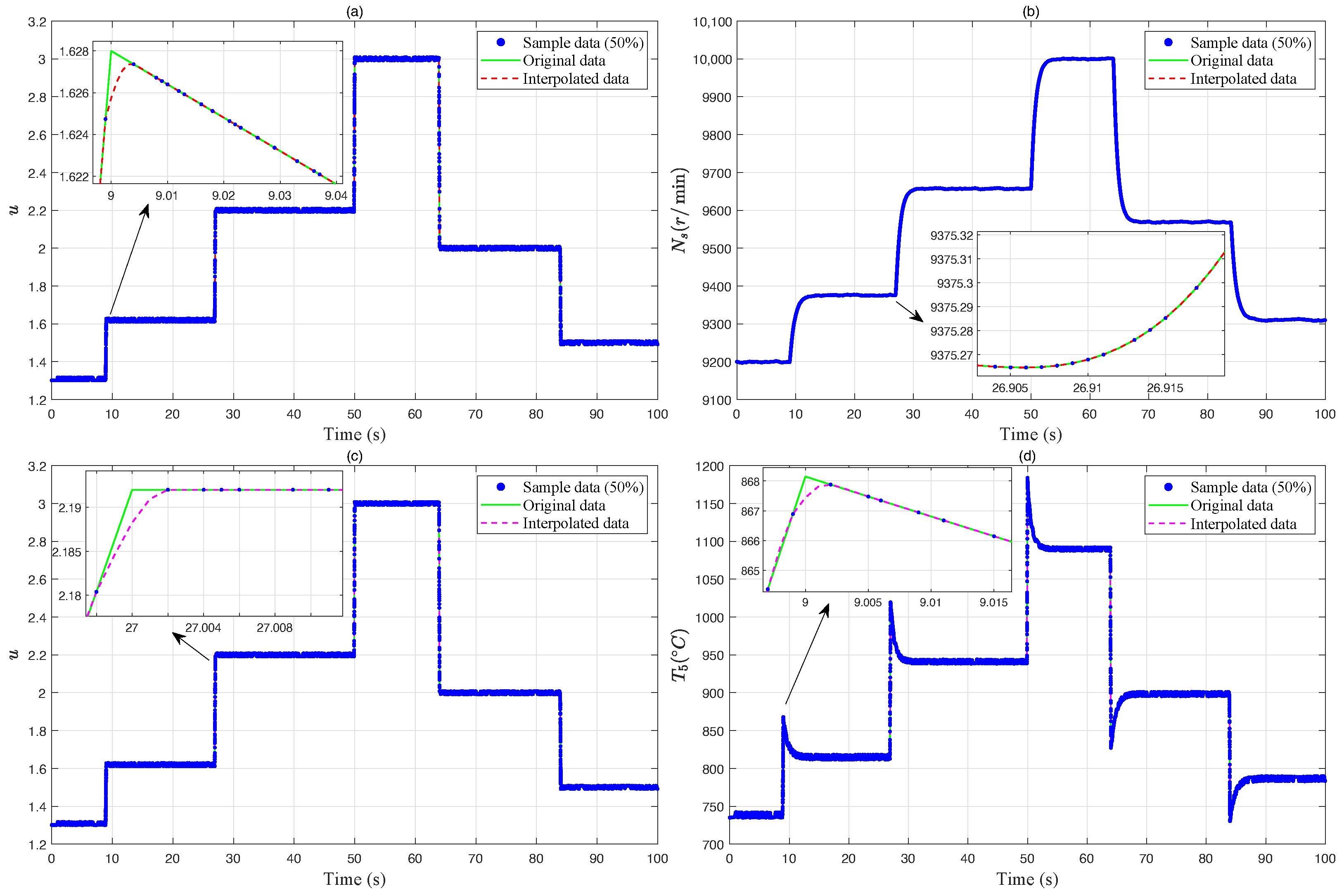
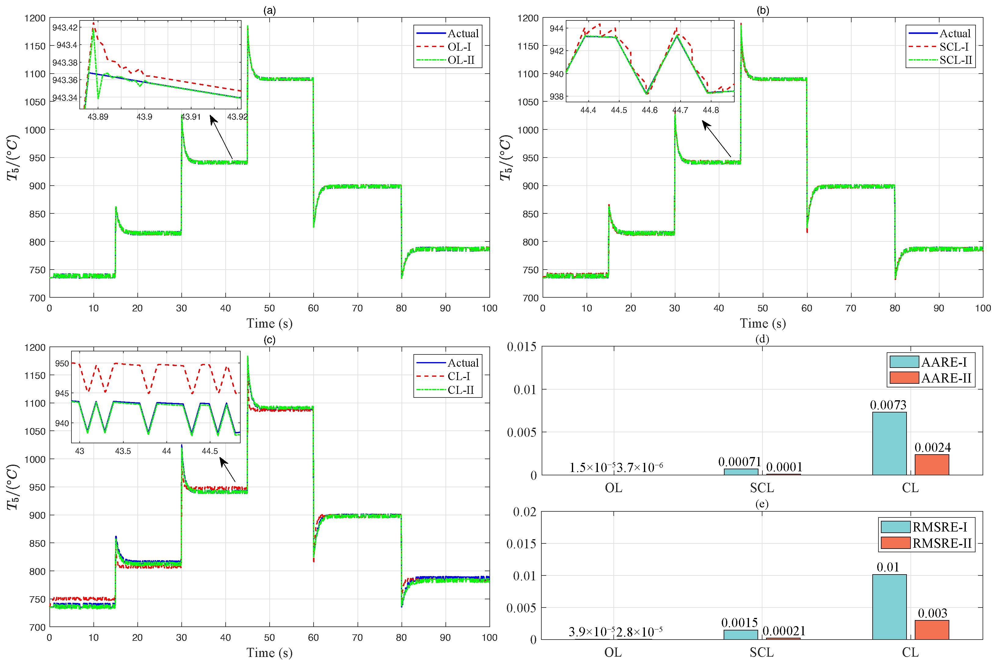
Based on the T-MATS configuration and the modeling procedure criteria, three data items are selected as optimal model inputs/outputs. Input $u_1$ is the u value of fuel flow to the engine. Output $y_1$ represents the aero-engine rotational speed $N_s$, and output $y_2$ is the exhaust gas temperature $T_5$. By using the ensemble modeling method proposed in this paper, simulation model prediction results are shown in Figure 6, Figure 7 and Figure 8. In the following figures, the inputs y of the NARX model are all actual measurement values in the OL mode, as shown in the upper part of Figure 4 above. In the SCL mode, the NARX model is corrected periodically using the real output as input during the running process. In this paper, the model is corrected every 50 steps, i.e., it is corrected per 5 s, as shown in the middle part of Figure 4 above. The inputs for the CL mode of NARX are all computed outputs ($\widehat{y}$) of the model, as shown in the bottom part of Figure 4 above.

Remark 2.

In the simulation experiments, we collect data from two experiments under identical conditions, with each dataset containing 100,000 data points. From the first experiment, 50,000 data points are randomly removed to construct Dataset I. The missing data in Dataset I are then imputed using the Makima method, yielding Dataset II, which contains 100,000 data points. Datasets I and II are used as training sets, respectively, while the data from the second experiment are used as the test set to evaluate the model accuracy. To validate this method, the prediction accuracy of models trained on Dataset I and Dataset II was compared using the AARE and RMSRE indicators. Figure 6, Figure 7 and Figure 8 and

Table 2. Speed/temperature models: missing vs. interpolated training data.

Parameter	Ratio	Index	Open-Loop		Semi-Closed Loop		Closed-Loop
			Origin	After	Origin	After	Origin	After
$N_s$	50%	AARE	2.8 × 10−6	7.8 × 10−7	6.9 × 10−5	1.9 × 10−5	0.0012	0.00056
		RMSRE	6.2 × 10−6	1.3 × 10−6	0.00017	3.7 × 10−5	0.0019	0.00068
$T_5$	50%	AARE	1.5 × 10−5	3.7 × 10−6	0.00071	0.0001	0.0073	0.0024
		RMSRE	3.9 × 10−5	2.8 × 10−5	0.0015	0.00021	0.01	0.003

show that the proposed method significantly reduces errors in 50% data loss scenario, offering a reference for engine modeling with sparse/missing data.

In Figure 7 and Figure 8, “xx-I” and “xx-II” represent the modeling results using Dataset I and Dataset II, respectively.

4.2. Experiments

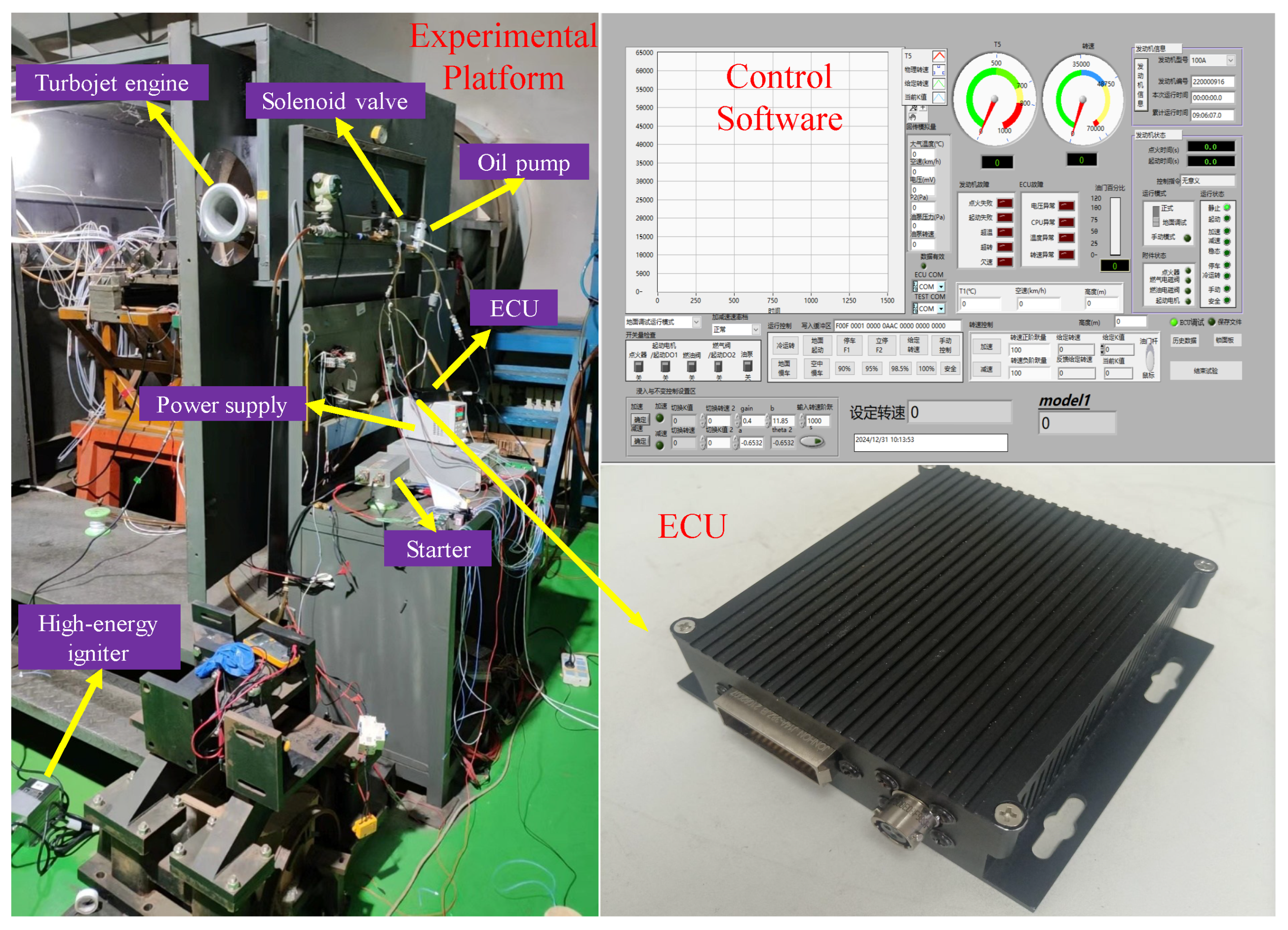
Regarding the above proposed modeling method, this paper takes the 100 E small-sized turbojet engine developed by the Institute of Engineering Thermophysics (IET) as the experimental validation platform. Figure 9 is the photo of the experimental validation platform, which mainly includes the turbojet engine body (equipped with a rotational speed sensor and an exhaust temperature sensor), ECU, oil pump, solenoid valve, starter, high-energy igniter, and power supply. The experimental procedures are as follows: (1) We use the control software shown in Figure 9 to give the ECU of the turbojet engine the start command and start the turbojet engine to the ground idle state (30,000 rpm). (2) After stabilizing for a period of time, we start collecting data. (3) We control the turbojet engine rotational speed from 35,000 rpm, 44,800 rpm, and 53,200 rpm to the full throttle state at 56,000 rpm. The first experimental data are recorded as the train data set. Under the condition that the inlet conditions remain basically unchanged, the second experiment is conducted according to the above procedure, and the experimental data of the second experiment are recorded as the test data set.

4.3. Experimental Data and Analysis

According to the model defined in Section 2, Formula (2), and the experimental setup configuration, three key data items were selected for experiments: input $u_1$ (oil pump motor voltage K value) and two outputs $y_1$ (aero-engine rotational speed $N_s$) and $y_2$ (exhaust gas temperature $T_5$).

Based on the above neural network architecture search method, the search scope is defined as follows: network training function (TF) selected from “trainlm”, “traincgp”, “traincgb”, and “trainscg”. Number of neuron nodes in the hidden layer $n_H\in [10,50]$. The hidden layer transfer function ($F_1$) is selected from “tansig”, “purelin”, “lossig”, “hardlim”, and “satlin”. Input delay order $n_{d1}\in [1,5]$. Output delay order $n_{d2}\in [1,20]$. The output layer transfer function ($F_2$) is fixed as “purelin”. Network structure hyperparameters are selected after more than 160 complete searches using the rotational speed and temperature data each, considering the accuracy, generalization ability, real-time performance, and convergence of the CL mode of the NARX model. The optimized network structure hyperparameters are shown in

Table 3. Network hyperparameters and training method.

	${\mathit{n}}_{\mathit{H}}$	${\mathit{F}}_1$	${\mathit{n}}_{\mathit{d}1}$	${\mathit{n}}_{\mathit{d}2}$	${\mathit{F}}_2$	TF
NARX1	28	Tansig	3	17	Purelin	Trainlm
NARX2	49	Tansig	3	12	Purelin	Trainlm

.

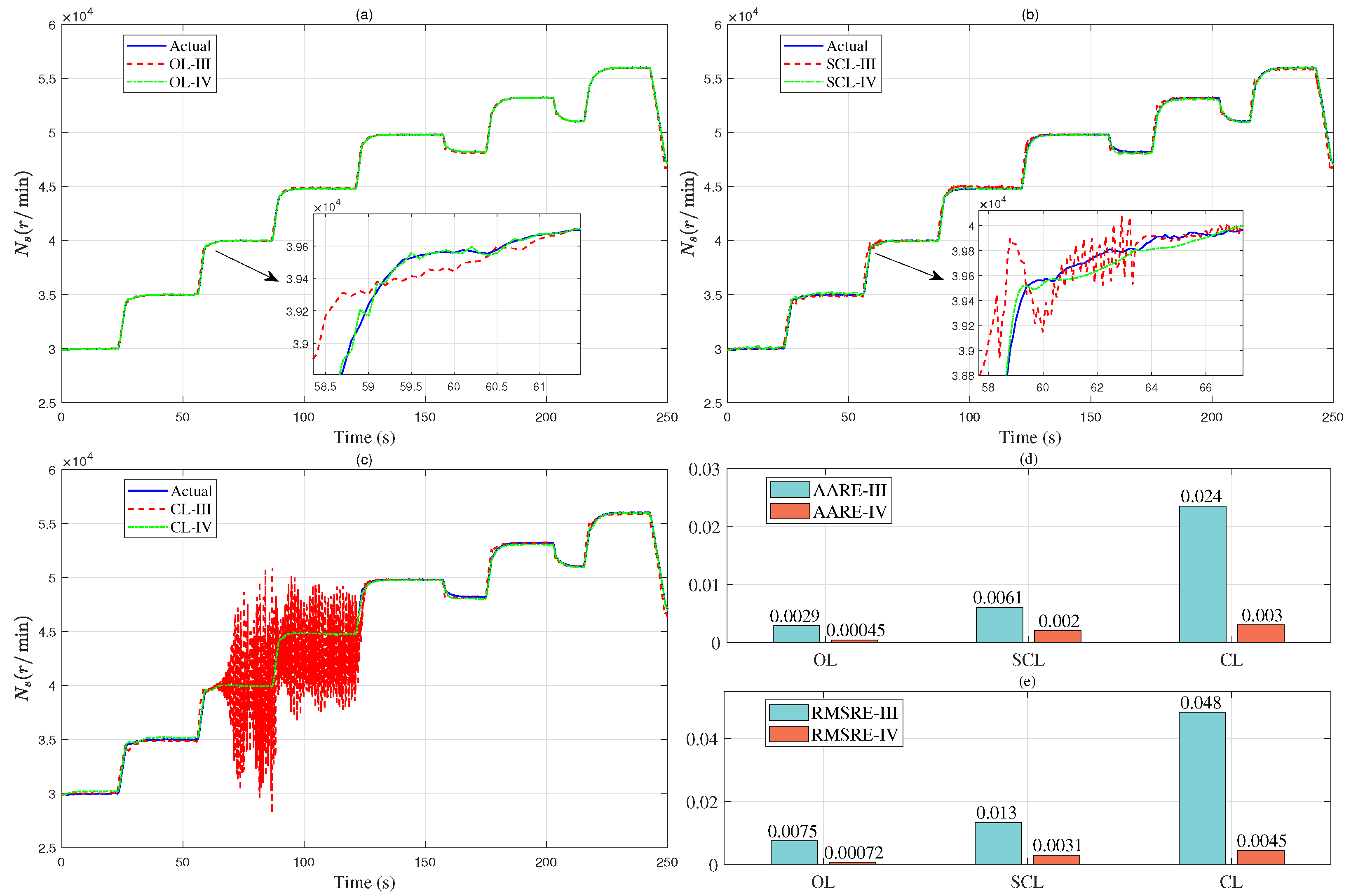
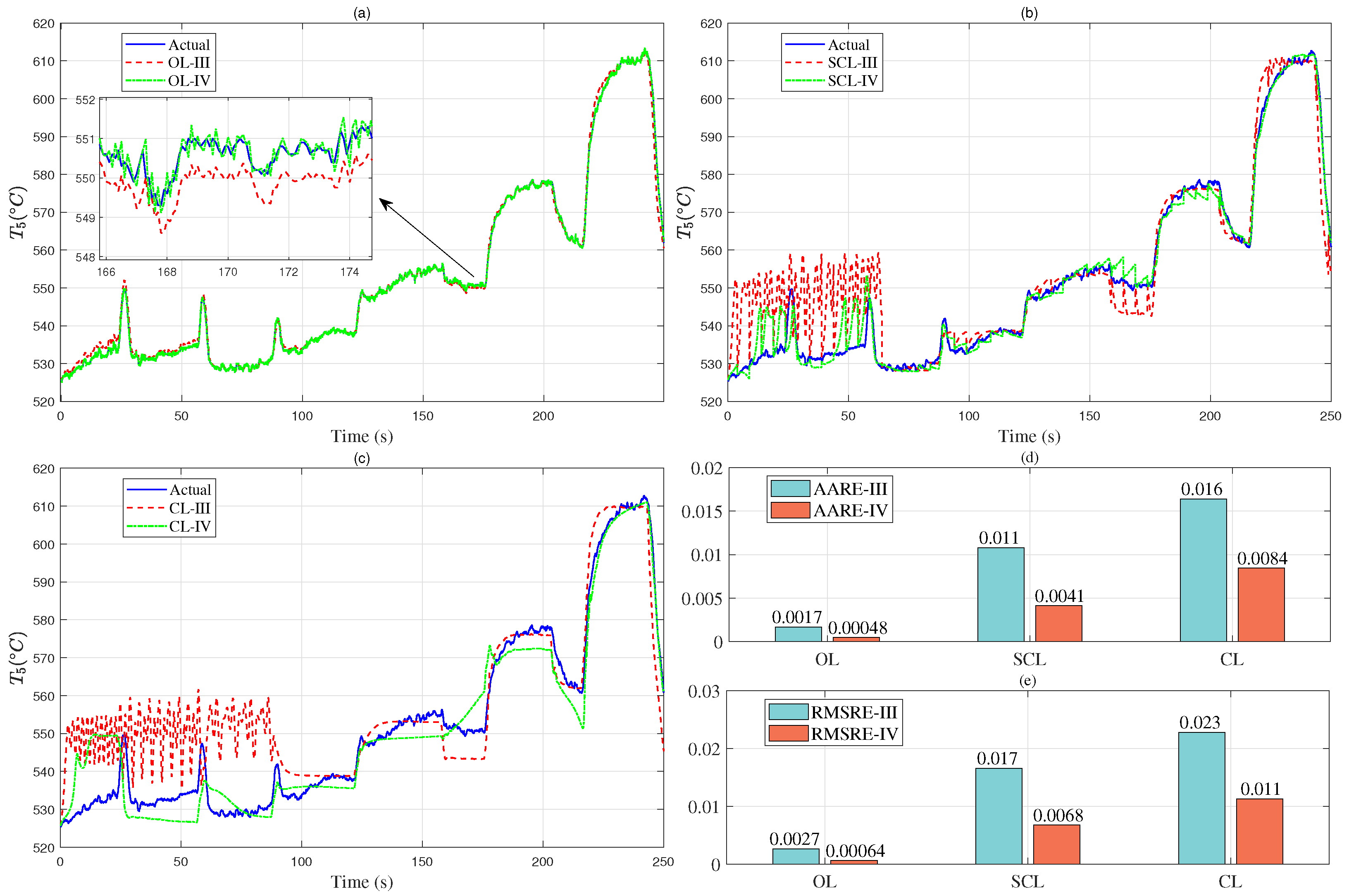
By using the ensemble modeling method proposed in this paper, model prediction results are shown in Figure 10, Figure 11, Figure 12, Figure 13, Figure 14 and Figure 15. In the following figures, the inputs of the NARX model are all actual measurement values in the OL mode, as shown in the upper part of Figure 4 above. In the SCL mode, the NARX model is corrected periodically using the real output as input during the running process. In this paper, the model is corrected every 50 steps, i.e., it is corrected per 5 s, as shown in the middle part of Figure 4 above. The inputs for the CL mode of NARX are all computed outputs ($\widehat{y}$) of the model, as shown in the bottom part of Figure 4 above. Actually, the OL mode is a one-step prediction. The SCL mode is a multi-step prediction. The CL mode only requires information about the initial state, and the subsequent outputs are all model outputs.

Remark 3.

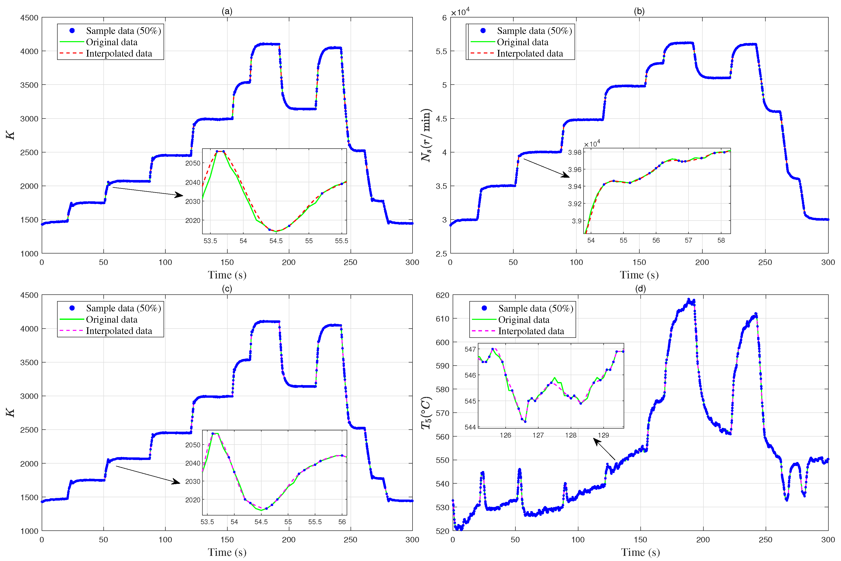
The experiment includes two cases. In the first case, 50% of the data are randomly missing, and the remaining 50% of the data are used for modeling. The actual experimental dataset consists of 3000 data points, from which 1500 data points are randomly extracted to create Dataset I with data loss. Subsequently, a new training Dataset II with 3000 data points is established by generating data based on the Makima method described above. In the second case, 80% of the data are randomly missing, and the remaining 20% are used for modeling. The actual dataset collected in the original experiment contains 3000 data points, from which 600 data points are randomly selected as Dataset III. A new training Dataset IV including 3000 data points, is constructed by the Makima method data described above. To validate the method’s efficacy, the generated datasets are contrasted with the original real data, as depicted in Figure 10 and Figure 13. The accuracy indexes of the model are also provided in

Table 4. Error indexes of Makima interpolation.

Parameter	Data Used for Interpolation	AARE	RMSRE
K	1500	0.00047	0.0009
	600	0.00104	0.00271
$N_s$	1500	0.00024	0.00034
	600	0.00049	0.001
$T_5$	1500	0.00031	0.00042
	600	0.00052	0.00081

.

Table 5. Comparison of error indexes between the rotational speed and exhaust gas temperature models trained on missing data and interpolated data.

Parameter	Ratio	Index	Open-Loop		Semi-Closed Loop		Closed-Loop
			Origin	After	Origin	After	Origin	After
$N_s$	50%	AARE	0.0016	0.00031	0.0039	0.0017	0.0043	0.0023
		RMSRE	0.0028	0.00076	0.0073	0.0025	0.0078	0.0035
	20%	AARE	0.0029	0.00045	0.00607	0.00204	0.02357	0.003
		RMSRE	0.0076	0.00072	0.01337	0.00305	0.04841	0.0045
$T_5$	50%	AARE	0.00055	0.00039	0.00584	0.00358	0.01339	0.00730
		RMSRE	0.00091	0.00054	0.00976	0.00625	0.01791	0.01171
	20%	AARE	0.00169	0.00048	0.01078	0.00412	0.01640	0.0084
		RMSRE	0.00267	0.00064	0.01658	0.00679	0.02283	0.01133

comprehensively illustrates that the generated data aligns well with the original real data, regardless of whether 50% or 80% of the data are missing, effectively resolving the issue of data sparsity.

Remark 4.

Figure 11, Figure 12, Figure 14 and Figure 15 show that the model can quickly converge to the actual data throughout the engine work process for predicting rotational speed, whether the engine operates in the OL, SCL, or CL mode. This result exhibits high accuracy, good generalization ability, and real-time performance. Specific indexes can be referred as the accuracy indexes shown in

Table 6. Time performance.

		First	Second	Third	Fourth	Fifth
		Execution	Execution	Execution	Execution	Execution
	Total Time (ms)	158.530	155.703	150.762	149.144	152.210
$N_s$	Iteration count	2719	2719	2719	2719	2719
	Average iteration time (ms)	0.0583	0.0573	0.0554	0.0549	0.0560
	Total Time (ms)	170.783	151.849	148.895	149.573	147.049
$T_5$	Iteration count	2724	2724	2724	2724	2724
	Average iteration time (ms)	0.0627	0.0557	0.0547	0.0549	0.0540

. Obviously, the OL mode exhibits the best performance in terms of AARE and RMSRE, followed by the SCL mode, while the CL mode shows the poorest overall performance. The reason lies in the fact that the CL mode only needs to know the initial state, and the subsequent outputs are all model outputs. This structure will lead to the accumulation and amplification of errors in long-term sequence prediction. The SCL mode corrects with actual values periodically. Thus, the degree of error accumulation is better than that of the CL mode. The OL mode is a single-step prediction closest to the training scenario, so it has the best accuracy. Additionally, we can see that the proposed modeling method has made obvious improvements.

In Figure 11 and Figure 12, “xx-I” and “xx-II” represent the modeling results using Dataset I and Dataset II, respectively. In Figure 14 and Figure 15, “xx-III” and “xx-IV” represent the modeling results using Dataset III and Dataset IV, respectively.

Remark 5.

Although the proposed ensemble modeling method is based on neural networks, its computational complexity is also acceptable. Even on an ordinary computer system, the configuration of the verification computing system is as follows: (1) CPU: 12th Gen Intel(R) Core (TM) i7-1265U 2.70 GHz; (2) Memory: 16.0 GB; (3) Operating System: Windows 10 64-bit operating system. The model runs in the MATLAB environment (version R2020a), and the model average iteration time is within approximately 0.05–0.06 milliseconds, which is much shorter than the control cycle of the aero-engine control system. Therefore, the model obtained by the method described in this paper can be used for precise monitoring, fault diagnosis, control optimization, and performance prediction of aero-engines.

Remark 6.

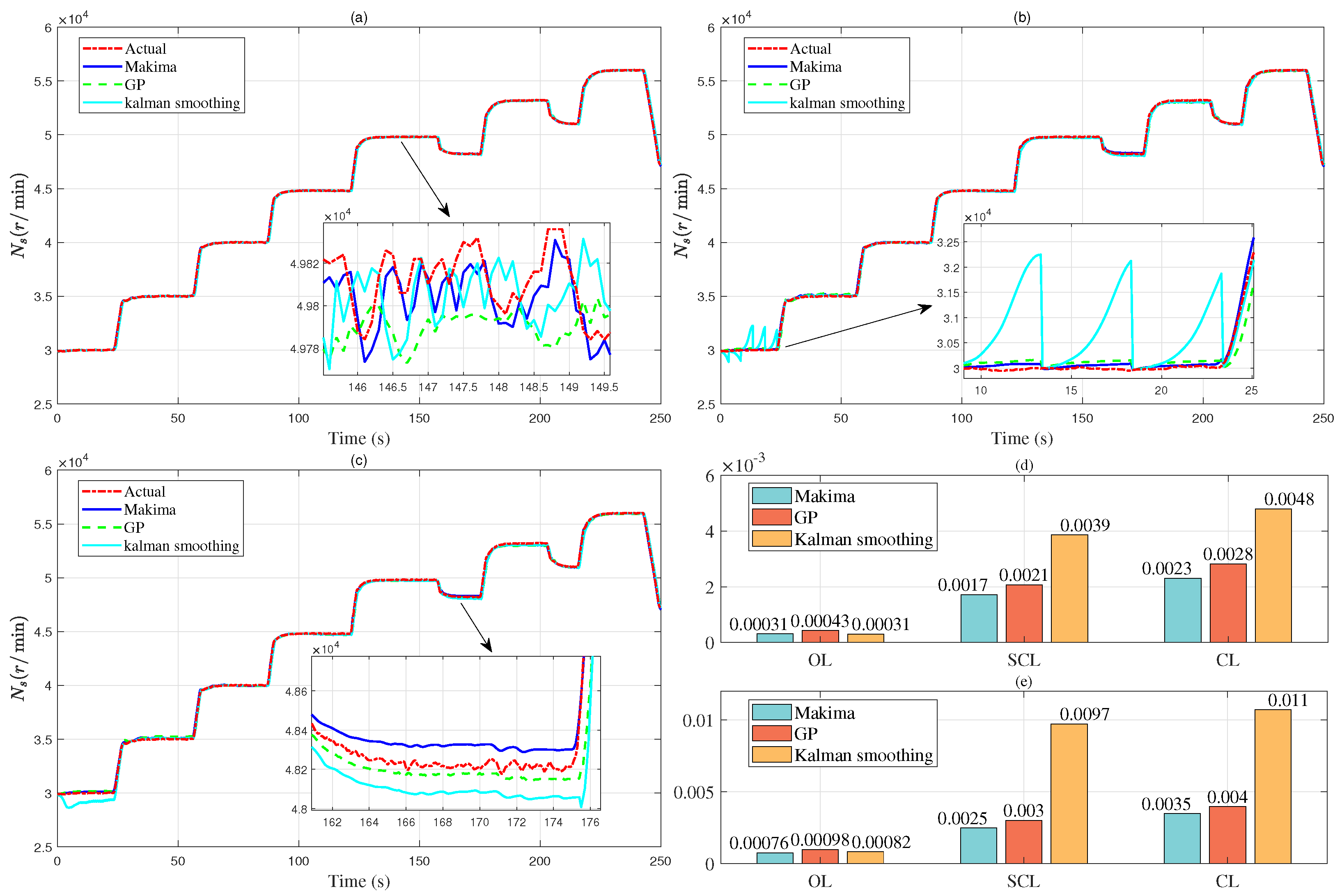
To evaluate the superiority of the proposed “Makima + NARX“ approach, two additional advanced interpolation methods, Gaussian Processes (GP) and Kalman smoothing, were introduced for comparison. Taking the case of 50% missing data as an example, we conducted a comparative analysis of the three modeling schemes, named “GP + NARX”, “Kalman + NARX“, and “Makima + NARX”. The experimental results are presented in Figure 16 and Figure 17. As observed, the predicted data generated by the speed prediction model and the gas temperature prediction model trained using all three methods exhibit good consistency with the actual data. However, under both SCL and CL modes, the models trained with the Makima method yield prediction values that are closer to the actual measurements.

5. Conclusions

To address the challenge of aero-engine ensemble modeling under sparse data conditions, this paper first analyzed the experimental data of a specific type of real aero-engine. The Makima method is used to interpolate and complete the sparse data, resolving the issue of data sparsity caused by sampling or transmission. Secondly, the NARX neural network is introduced as the computational structure of the model. Based on data specificity, the ANAS method is used to search for model hyperparameters, enhancing model performance. Thirdly, an ensemble modeling method based on the Makima method, the NARX model, and the ANAS method is proposed to realize high-precision modeling of the aero-engine’s entire process from idle to full throttle. Finally, the proposed method is verified by simulations and experiments. The results fully demonstrated the correctness of the method proposed in this paper. THe model obtained by this method possesses high accuracy, good generalization ability, and real-time performance.

References

1. Brunton, S.L.; Nathan Kutz, J.; Manohar, K.; Aravkin, A.Y.; Morgansen, K.; Klemisch, J.; Goebel, N.; Buttrick, J.; Poskin, J.; Blom-Schieber, A.W.; et al. Data-driven aerospace engineering: Reframing the industry with machine learning. AIAA J. 2021, 59, 2820–2847. [Google Scholar] [CrossRef]
2. Qian, C.; Sheng, H.; Zhang, T. An improved nonlinear onboard adaptive model for aero-engine performance control. Chin. J. Aeronaut. 2023, 36, 317–334. [Google Scholar]
3. Wang, Y.; Liu, F.; Xi, F.; Wei, B.; Duan, D.; Cai, Z.; Si, S. Data Driven Comprehensive Performance Evaluation of Aeroengines: A Network Dynamic Approach. Engineering 2025, 46, 292–305. [Google Scholar] [CrossRef]
4. Zhang, H.; Chen, X.; Chen, W.; Shen, Z. Collaborative sparse classification for aero-engine’s gear hub crack diagnosis. Mech. Syst. Signal Process. 2020, 141, 106426. [Google Scholar] [CrossRef]
5. Yao, R.; Jiang, H.; Liu, Y.; Wang, X.; Shao, H.; Jiang, W. Deep Sparse Representation Classification for Aeroengine Inter-shaft Bearing Fault Diagnosis. In Proceedings of the 2024 IEEE International Conference on Prognostics and Health Management (ICPHM), Spokane, WA, USA, 17–19 June 2024; pp. 167–173. [Google Scholar]
6. Wei, Z.; Zhang, S.; Jafari, S.; Nikolaidis, T. Gas turbine aero-engines real time on-board modelling: A review, research challenges, and exploring the future. Prog. Aerosp. Sci. 2020, 121, 100693. [Google Scholar] [CrossRef]
7. Sun, R.Q.; Han, X.B.; Chen, Y.X.; Gou, L.F. Hyperelliptic Kalman filter-based aeroengine sensor fault FDIA system under multi-source uncertainty. Aerosp. Sci. Technol. 2023, 132, 108058. [Google Scholar] [CrossRef]
8. Zhou, X.; Huang, J.; Lu, F.; Zhou, W.; Liu, P. A novel compound fault-tolerant method based on online sequential extreme learning machine with cycle reservoir for turbofan engine direct thrust control. Aerosp. Sci. Technol. 2023, 132, 108059. [Google Scholar] [CrossRef]
9. Yang, X.; Jian, M.; Dong, W.; Xu, Q. Simulation of the secondary air system of turbofan engines: Insights from 1D–3D modeling. Chin. J. Aeronaut. 2023, 36, 231–245. [Google Scholar] [CrossRef]
10. Shuwei, P.; Qiuhong, L.; Zhang, H. A new online modelling method for aircraft engine state space model. Chin. J. Aeronaut. 2020, 33, 1756–1773. [Google Scholar] [CrossRef]
11. Chen, H.; Cai, C.; Jiang, S.; Zhang, H. Numerical modeling on installed performance of turbofan engine with inlet ejector. Aerosp. Sci. Technol. 2021, 112, 106590. [Google Scholar] [CrossRef]
12. Liu, F.Z.; Shi, Y.; Sun, C.Y.; Sun, X.M. Improved real-time H∞ control for aero-engines based on the equilibrium manifold expansion model. J. Frankl. Inst. 2024, 361, 107342. [Google Scholar] [CrossRef]
13. Liu, J.; Wang, X.; Zhu, M.; Miao, K. Multivariable adaptive control method for turbofan engine with dynamic and input uncertainties. J. Eng. Gas Turbines Power 2021, 143, 071027. [Google Scholar] [CrossRef]
14. Huang, D.; Zhou, D.; Jia, X.; Hao, J.; Fang, Q. Gas path deterioration assessment for turbofan engines based on stochastic dynamics responses in the thermodynamic cycle. Mech. Syst. Signal Process. 2022, 178, 109314. [Google Scholar] [CrossRef]
15. Wang, C.; Yu, Z.; Du, X.; Sun, X. An improved high-fidelity adaptive model for integrated inlet-engine-nozzle based on mechanism-data fusion. Chin. J. Aeronaut. 2024, 37, 190–207. [Google Scholar] [CrossRef]
16. L’Erario, G.; Fiorio, L.; Nava, G.; Bergonti, F.; Mohamed, H.A.O.; Benenati, E.; Traversaro, S.; Pucci, D. Modeling, identification and control of model jet engines for jet powered robotics. IEEE Robot. Autom. Lett. 2020, 5, 2070–2077. [Google Scholar] [CrossRef]
17. Wei, Z.; Jafari, S.; Zhang, S.; Nikolaidis, T. Hybrid Wiener model: An on-board approach using post-flight data for gas turbine aero-engines modelling. Appl. Therm. Eng. 2021, 184, 116350. [Google Scholar] [CrossRef]
18. Pan, M.; Wang, H.; Huang, J. T–S Fuzzy Modeling for Aircraft Engines: The Clustering and Identification Approach. Energies 2019, 12, 3284. [Google Scholar] [CrossRef]
19. Singh, D.J.; Verma, N.K.; Ghosh, A.K.; Malagaudanavar, A. An application of interval type-2 fuzzy model based control system for generic aircraft. Appl. Soft Comput. 2022, 121, 108721. [Google Scholar] [CrossRef]
20. Wang, W.; Peng, J.; Zhang, Y. Modeling and control for an aero-engine based on the takagi-sugeno fuzzy model. Aerospace 2023, 10, 523. [Google Scholar] [CrossRef]
21. Pan, M.; Wang, H.; Zhang, C.; Xu, Y. Fuzzy Control for Aircraft Engine: Dynamics Clustering Modeling, Compensation and Hardware-in-Loop Experimental Verification. Aerospace 2024, 11, 610. [Google Scholar] [CrossRef]
22. De Giorgi, M.G.; Quarta, M. Hybrid multigene genetic programming-artificial neural networks approach for dynamic performance prediction of an aeroengine. Aerosp. Sci. Technol. 2020, 103, 105902. [Google Scholar] [CrossRef]
23. De Giorgi, M.G.; Strafella, L.; Ficarella, A. Neural nonlinear autoregressive model with exogenous input (NARX) for turboshaft aeroengine fuel control unit model. Aerospace 2021, 8, 206. [Google Scholar] [CrossRef]
24. Ferdaus, M.M.; Anavatti, S.G.; Pratama, M.; Garratt, M.A. Towards the use of fuzzy logic systems in rotary wing unmanned aerial vehicle: A review. Artif. Intell. Rev. 2020, 53, 257–290. [Google Scholar] [CrossRef]
25. Lv, C.; Chang, J.; Bao, W.; Yu, D. Recent research progress on airbreathing aero-engine control algorithm. Propuls. Power Res. 2022, 11, 1–57. [Google Scholar] [CrossRef]
26. Lei, B.; Shen, N.; Ji, D.; Ouyang, R.; Yang, L.; Liu, Q.; Gao, B.; Wang, Z. A Comprehensive Review of Key Technologies for Enhancing the Reliability of Aero-Engines. IEEE Access 2024, 12, 148315–148331. [Google Scholar] [CrossRef]
27. Yin, S.; Ding, S.X.; Xie, X.; Luo, H. A review on basic data-driven approaches for industrial process monitoring. IEEE Trans. Ind. Electron. 2014, 61, 6418–6428. [Google Scholar] [CrossRef]
28. Castillo, I.G.; Loboda, I.; Pérez Ruiz, J.L. Data-driven models for gas turbine online diagnosis. Machines 2021, 9, 372. [Google Scholar] [CrossRef]
29. Lodygowski, T.; Szrama, S. Unsupervised Classification and Remaining Useful Life Prediction for Turbofan Engines Using Autoencoders and Gaussian Mixture Models: A Comprehensive Framework for Predictive Maintenance. Appl. Sci. 2025, 15, 7884. [Google Scholar] [CrossRef]
30. Szrama, S. Optimizing aircraft engine longevity: A comparative framework for dynamically adaptive predictive maintenance using autoencoders, LSTMs, and Gaussian processes. Eng. Appl. Artif. Intell. 2025, 156, 111199. [Google Scholar] [CrossRef]
31. Szrama, S. Turbofan engine health status prediction with neural network pattern recognition and automated feature engineering. Aircr. Eng. Aerosp. Technol. Int. J. 2024, 96, 19–26. [Google Scholar] [CrossRef]
32. Xu, C.; Li, W.; Zhao, Y. A Novel Fused NARX-Driven Digital Twin Model for Aeroengine Gas Path Parameter Prediction. IEEE Trans. Ind. Inform. 2024, 20, 6280–6288. [Google Scholar] [CrossRef]
33. Thudumu, S.; Branch, P.; Jin, J.; Singh, J. A comprehensive survey of anomaly detection techniques for high dimensional big data. J. Big Data 2020, 7, 42. [Google Scholar] [CrossRef]
34. Hou, Z.G.; Wang, H.W.; Lv, S.L.; Xiong, M.L.; Peng, K. Siamese multiscale residual feature fusion network for aero-engine bearing fault diagnosis under small-sample condition. Meas. Sci. Technol. 2022, 34, 035109. [Google Scholar] [CrossRef]
35. Ding, P.; Xu, Y.; Sun, X.M. Multi-task Learning for Aero-engine Bearing Fault Diagnosis with Limited Data. IEEE Trans. Instrum. Meas. 2024, 73, 3520111. [Google Scholar] [CrossRef]
36. Yu, B.; Shu, W.; Cao, C. A novel modeling method for aircraft engine using nonlinear autoregressive exogenous (NARX) models based on wavelet neural networks. Int. J. Turbo-Jet-Engines 2018, 35, 161–169. [Google Scholar] [CrossRef]
37. Liu, Q.; Chen, W.; Hu, H.; Zhu, Q.; Xie, Z. An optimal NARX neural network identification model for a magnetorheological damper with force-distortion behavior. Front. Mater. 2020, 7, 10. [Google Scholar] [CrossRef]
38. Cheng, A.; Low, Y.M. Improved generalization of NARX neural networks for enhanced metamodeling of nonlinear dynamic systems under stochastic excitations. Mech. Syst. Signal Process. 2023, 200, 110543. [Google Scholar] [CrossRef]
39. Kuranga, C.; Pillay, N. A comparative study of nonlinear regression and autoregressive techniques in hybrid with particle swarm optimization for time-series forecasting. Expert Syst. Appl. 2022, 190, 116163. [Google Scholar] [CrossRef]
40. Malik, M.F.; Chang, C.L.; Chaudhary, N.I.; Khan, Z.A.; Kausar Kiani, A.; Shu, C.M.; Raja, M.A.Z. Swarming intelligence heuristics for fractional nonlinear autoregressive exogenous noise systems. Chaos Solitons Fractals 2023, 167, 113085. [Google Scholar] [CrossRef]
41. Ibrahem, I.M.; Akhrif, O.; Moustapha, H.; Staniszewski, M. Nonlinear generalized predictive controller based on ensemble of NARX models for industrial gas turbine engine. Energy 2021, 230, 120700. [Google Scholar] [CrossRef]
42. López, G.; Arboleya, P. Short-term wind speed forecasting over complex terrain using linear regression models and multivariable LSTM and NARX networks in the Andes Mountains, Ecuador. Renew. Energy 2022, 183, 351–368. [Google Scholar] [CrossRef]
43. Zhou, J.; Li, J. An efficient time-variant reliability analysis strategy embedding the NARX neural network of response characteristics prediction into probability density evolution method. Mech. Syst. Signal Process. 2023, 200, 110516. [Google Scholar] [CrossRef]
44. Kelley, J.; Hagan, M.T. Comparison of neural network NARX and NARMAX models for multi-step prediction using simulated and experimental data. Expert Syst. Appl. 2024, 237, 121437. [Google Scholar] [CrossRef]
45. Schreiber, J.F.; Sausen, A.; De Campos, M.; Sausen, P.S.; Ferreira Filho, M.T.D.S. Data imputation techniques applied to the smart grids environment. IEEE Access 2023, 11, 31931–31940. [Google Scholar] [CrossRef]
46. Liu, Y.; Zhang, Y.A.; Zeng, M.; Zhao, J. A novel shape-based averaging algorithm for time series. Eng. Appl. Artif. Intell. 2023, 126, 107098. [Google Scholar] [CrossRef]
Figure 1. Diagram of the ensemble modeling method under sparse data.
Aerospace 12 00804 g001
Figure 2. Comparisons of Makima, Hermite, and Cubic Splines Interpolation in Case 1 (a) and Case 2 (b).
Aerospace 12 00804 g002
Figure 3. Integrated modeling planning schematics.
Aerospace 12 00804 g003
Figure 4. Three work modes of NARX.
Aerospace 12 00804 g004
Figure 5. Process of the ANAS method.
Aerospace 12 00804 g005
Figure 6. Makima interpolation results using 50% data. (a) Interpolation u (Prediction N s ). (b) Interpolation N s . (c) Interpolation u (Prediction T 5 ). (d) Interpolation T 5 .
Aerospace 12 00804 g006
Figure 7. Comparison of rotational speed prediction model using 50% data and interpolation data. (a) Open loop. (b) Semi-closed loop. (c) Closed loop. (d) Model accuracy: AARE. (e) Model accuracy: RMSRE.
Aerospace 12 00804 g007
Figure 8. Comparison of exhaust gas temperature prediction model using 50% data and interpolation data. (a) Open loop. (b) Semi-closed loop. (c) Closed loop. (d) Model accuracy: AARE. (e) Model accuracy: RMSRE.
Aerospace 12 00804 g008
Figure 9. Experimental setup and control software.
Aerospace 12 00804 g009
Figure 10. Makima interpolation results using 50% data. (a) Interpolation K (Prediction N s ). (b) Interpolation N s . (c) Interpolation K (Prediction T 5 ). (d) Interpolation T 5 .
Aerospace 12 00804 g010
Figure 11. Comparison of rotational speed prediction model using 50% data and interpolation data. (a) Open loop. (b) Semi-closed loop. (c) Closed loop. (d) Model accuracy: AARE. (e) Model accuracy: RMSRE.
Aerospace 12 00804 g011
Figure 12. Comparison of exhaust gas temperature prediction model using 50% data and interpolation data. (a) Open loop. (b) Semi-closed loop. (c) Closed loop. (d) Model accuracy: AARE. (e) Model accuracy: RMSRE.
Aerospace 12 00804 g012
Figure 13. Makima interpolation results using 20% data. (a) Interpolation K (Prediction N s ). (b) Interpolation N s . (c) Interpolation K (Prediction T 5 ). (d) Interpolation T 5 .
Aerospace 12 00804 g013
Figure 14. Comparison of exhaust rotational speed prediction model using 20% data and interpolation data. (a) Open loop. (b) Semi-closed loop. (c) Closed loop. (d) Model accuracy: AARE. (e) Model accuracy: RMSRE.
Aerospace 12 00804 g014
Figure 15. Comparison of exhaust gas temperature prediction model using 20% data and interpolation data. (a) Open loop. (b) Semi-closed loop. (c) Closed loop. (d) Model accuracy: AARE. (e) Model accuracy: RMSRE.
Aerospace 12 00804 g015
Figure 16. Rotational speed prediction model based on different interpolation methods. (a) Open loop. (b) Semi-closed loop. (c) Closed loop. (d) Model accuracy: AARE. (e) Model accuracy: RMSRE.
Aerospace 12 00804 g016
Figure 17. Exhaust gas temperature prediction model based on different interpolation methods. (a) Open loop. (b) Semi-closed loop. (c) Closed loop. (d) Model accuracy: AARE. (e) Model accuracy: RMSRE.
Aerospace 12 00804 g017