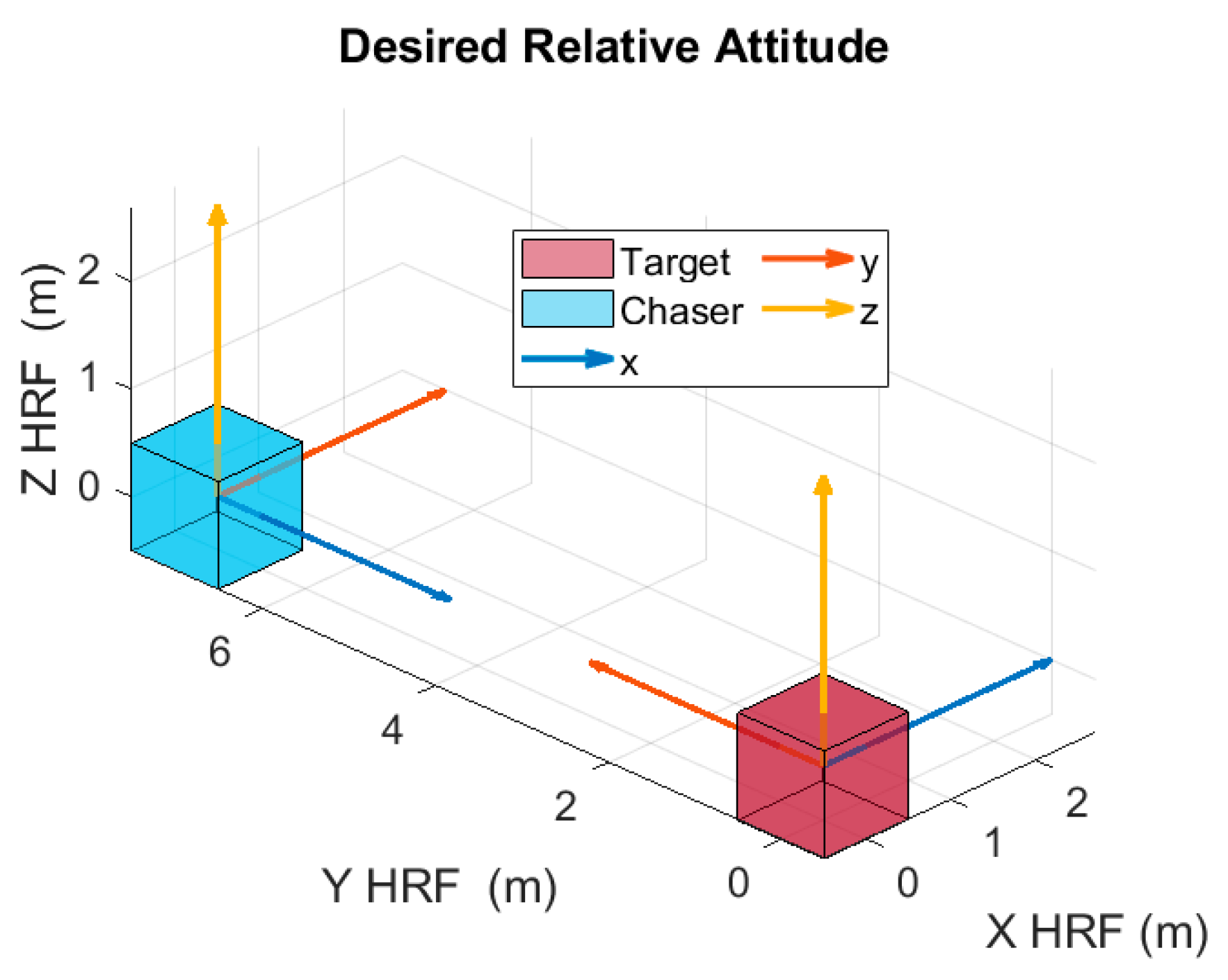
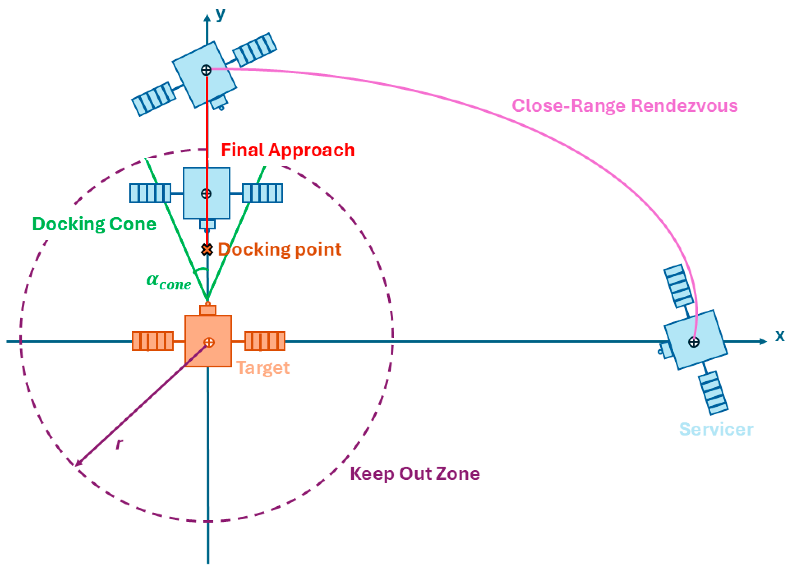
Figure 1.
A 2D representation of the considered rendezvous scenario: Close-Range Rendezvous and Final Approach phases.
Figure 1.
A 2D representation of the considered rendezvous scenario: Close-Range Rendezvous and Final Approach phases.
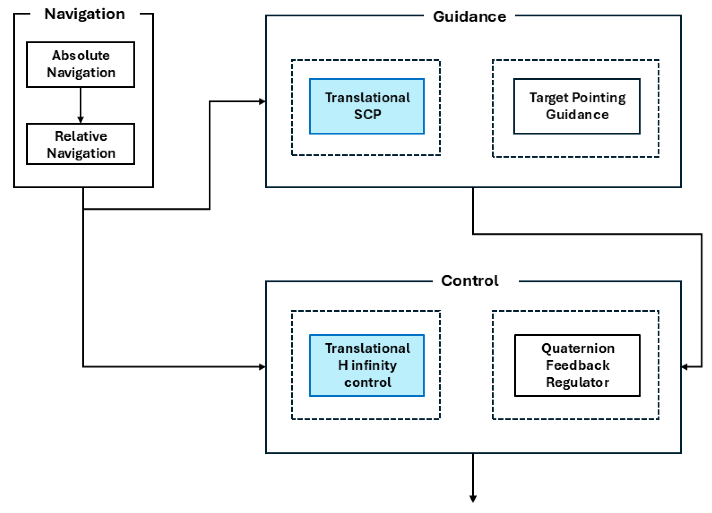
Figure 2.
Schematic representation of Guidance, Navigation and Control architecture for the Close-Range phase. The blue blocks indicate the original functions proposed in this paper and described in the following.
Figure 2.
Schematic representation of Guidance, Navigation and Control architecture for the Close-Range phase. The blue blocks indicate the original functions proposed in this paper and described in the following.
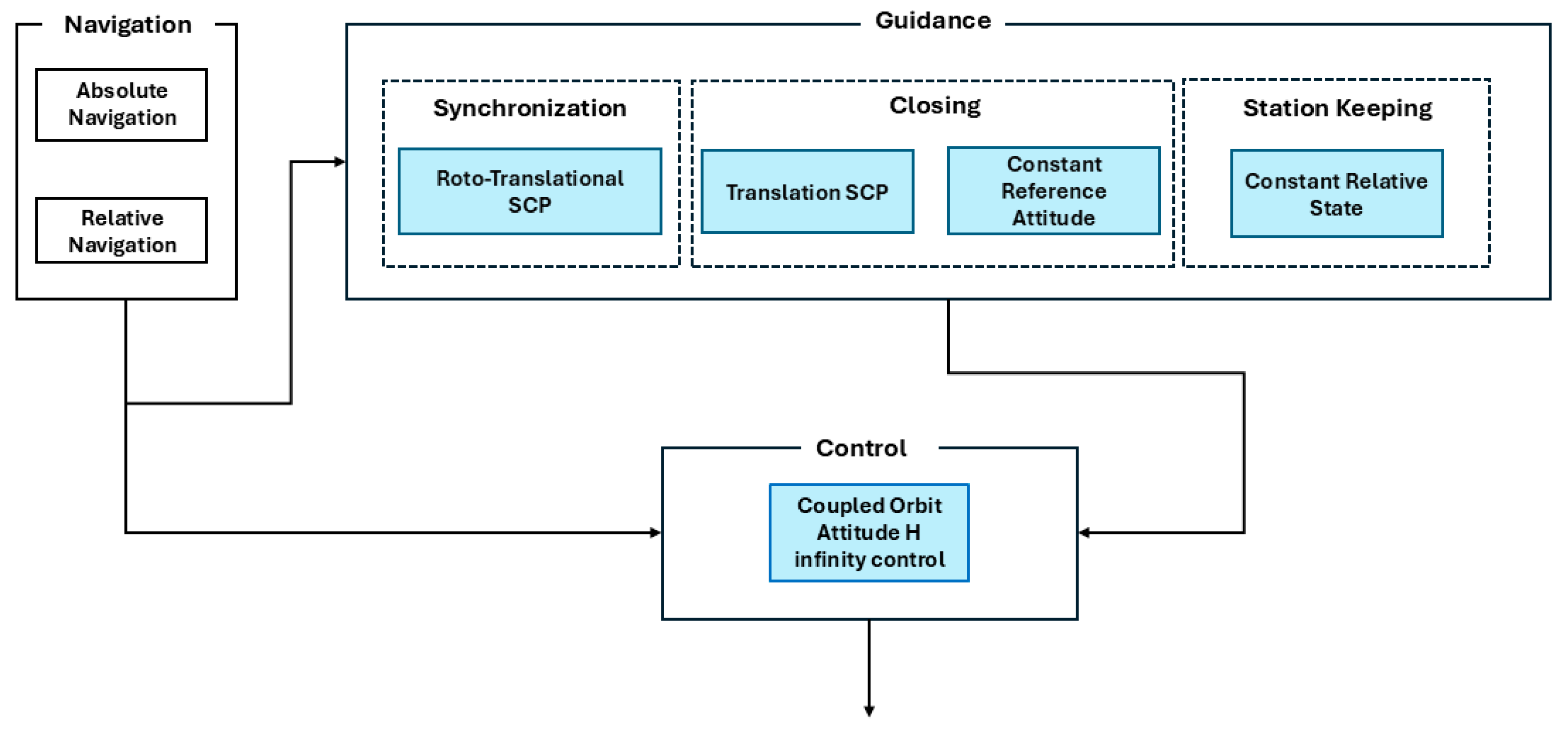
Figure 3.
Schematic representation of Guidance, Navigation and Control architecture for the Final Approach phase. The blue blocks indicate the original functions proposed in this paper and described in the following.
Figure 3.
Schematic representation of Guidance, Navigation and Control architecture for the Final Approach phase. The blue blocks indicate the original functions proposed in this paper and described in the following.
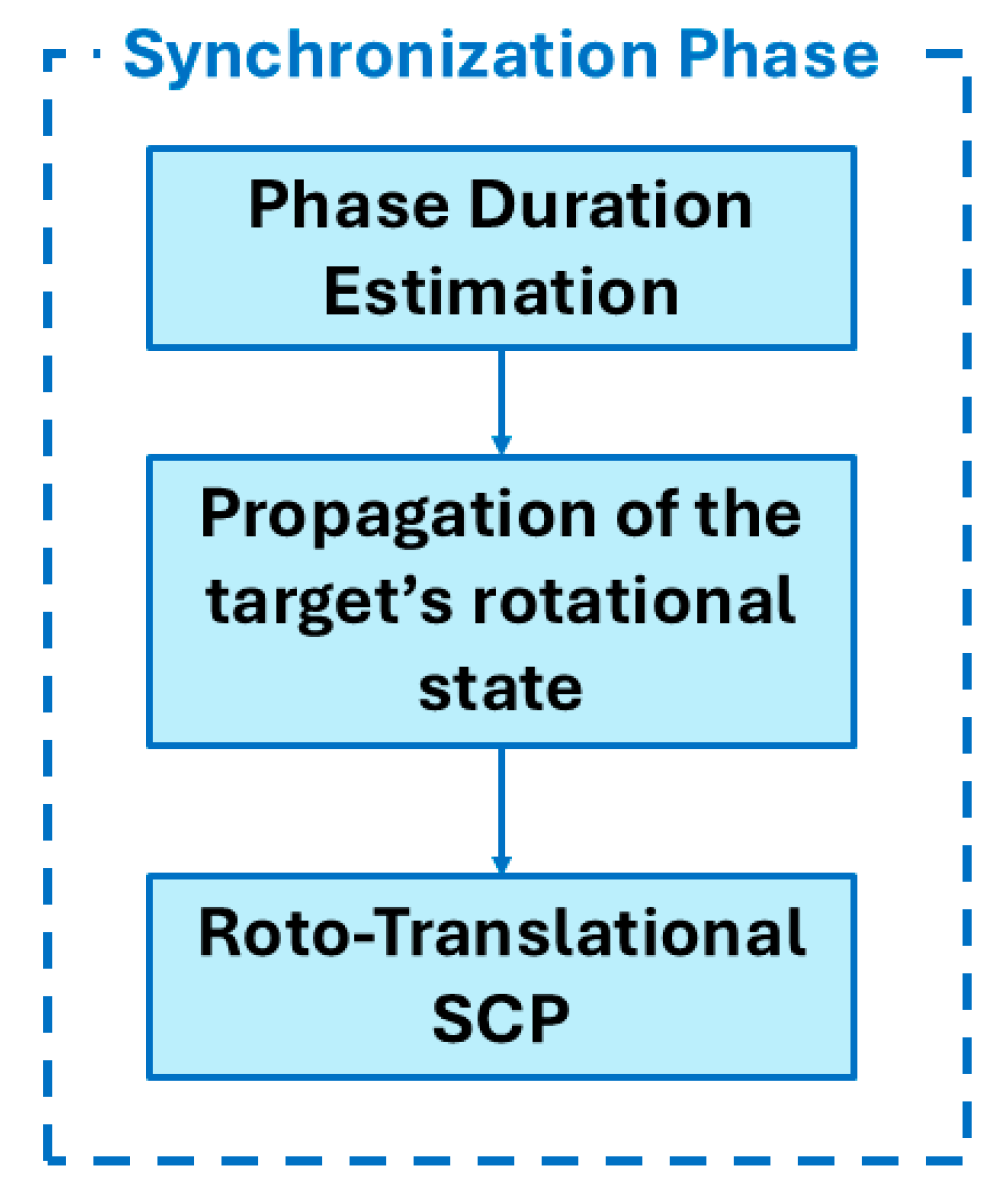
Figure 4.
Guidance functions implemented during the Synchronization Phase.
Figure 4.
Guidance functions implemented during the Synchronization Phase.
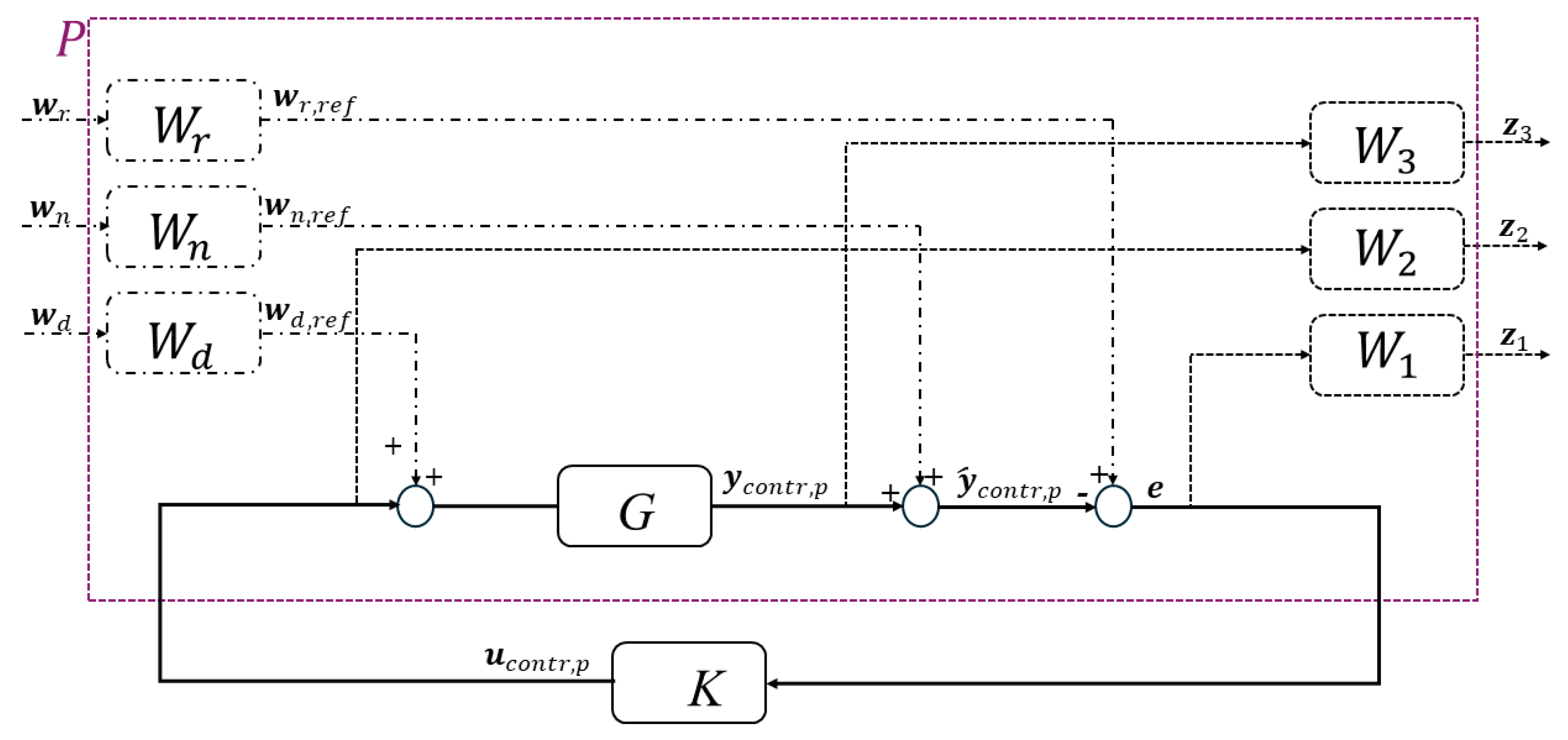
Figure 5.
Block diagram of a generic mixed sensitivity H infinity controller [
34].
Figure 5.
Block diagram of a generic mixed sensitivity H infinity controller [
34].
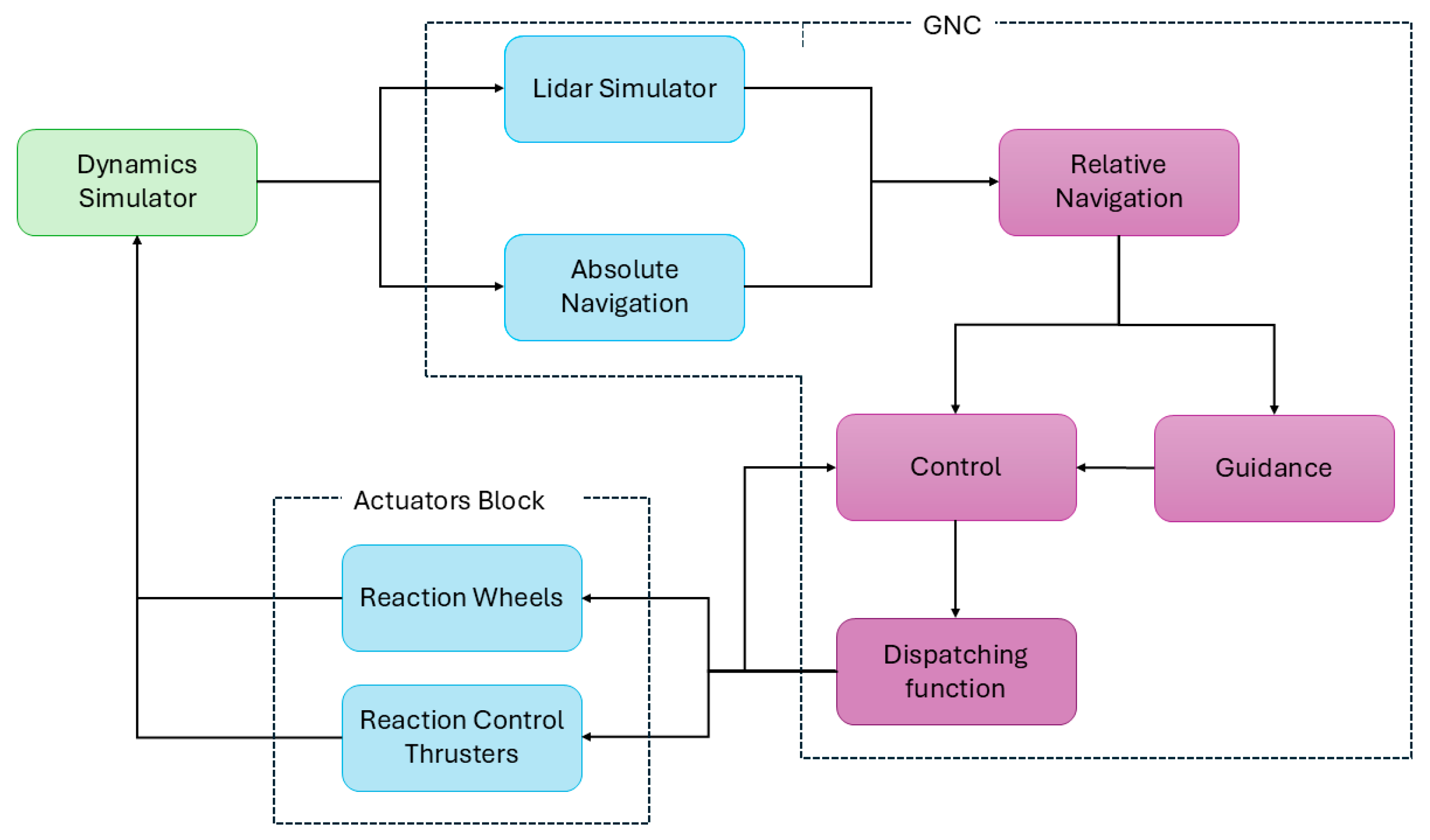
Figure 6.
Block diagram of the simulation environment. The blue blocks represent the sensors and actuators, the green block corresponds to the numerical propagator, and the violet blocks indicate the functional components.
Figure 6.
Block diagram of the simulation environment. The blue blocks represent the sensors and actuators, the green block corresponds to the numerical propagator, and the violet blocks indicate the functional components.
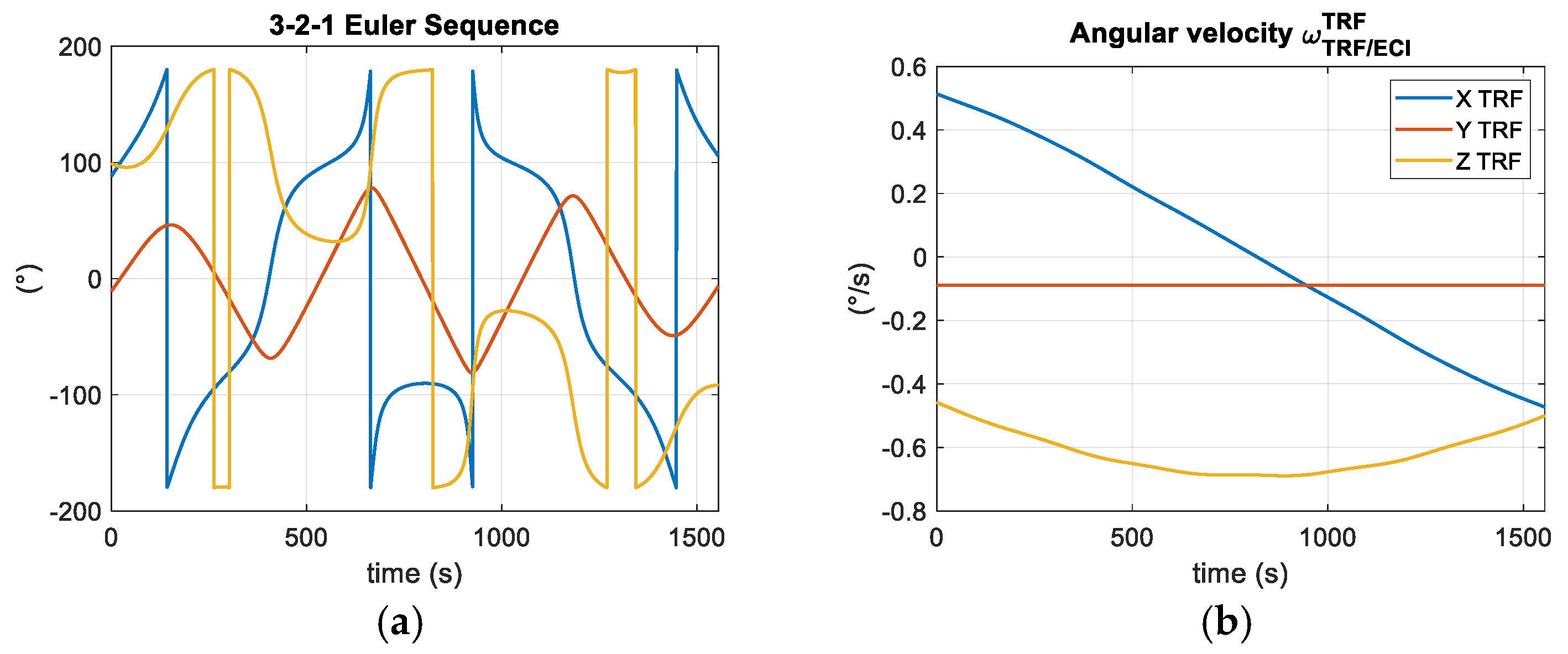
Figure 8.
(a) Time history of the relative attitude of the target with respect to HRF. To better understand the relative attitude variations, a 3-2-1 Euler Sequence representation is chosen: blue represents the first rotation, (αTRF/HRF); red the second (βTRF/HRF) and yellow the third rotation (γTRF/HRF). (b) Time history of the target angular velocity.
Figure 9.
Nominal Translation Trajectory: (a) Relative Position expressed in HRF and (b) Relative Velocity expressed in HRF and (c) Relative Position expressed in TRF.
Figure 9.
Nominal Translation Trajectory: (a) Relative Position expressed in HRF and (b) Relative Velocity expressed in HRF and (c) Relative Position expressed in TRF.
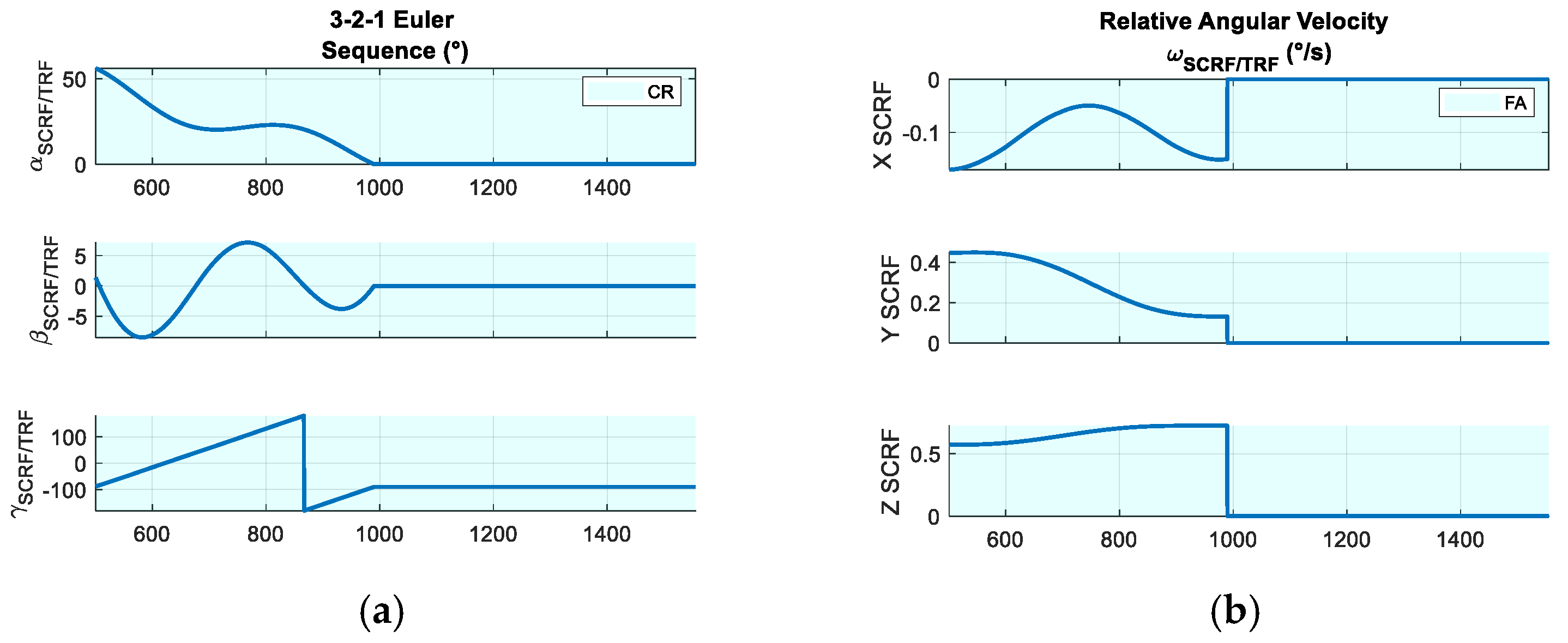
Figure 10.
Nominal Rotational Trajectory: (a) Relative Attitude of the chaser with respect to the target (3-2-1 Euler Sequence) and (b) Relative Angular Velocity expressed in SCRF.
Figure 10.
Nominal Rotational Trajectory: (a) Relative Attitude of the chaser with respect to the target (3-2-1 Euler Sequence) and (b) Relative Angular Velocity expressed in SCRF.
Figure 11.
Constraints: (a) KOZ, (b) Target Visibility and (c) Docking Cone.
Figure 11.
Constraints: (a) KOZ, (b) Target Visibility and (c) Docking Cone.
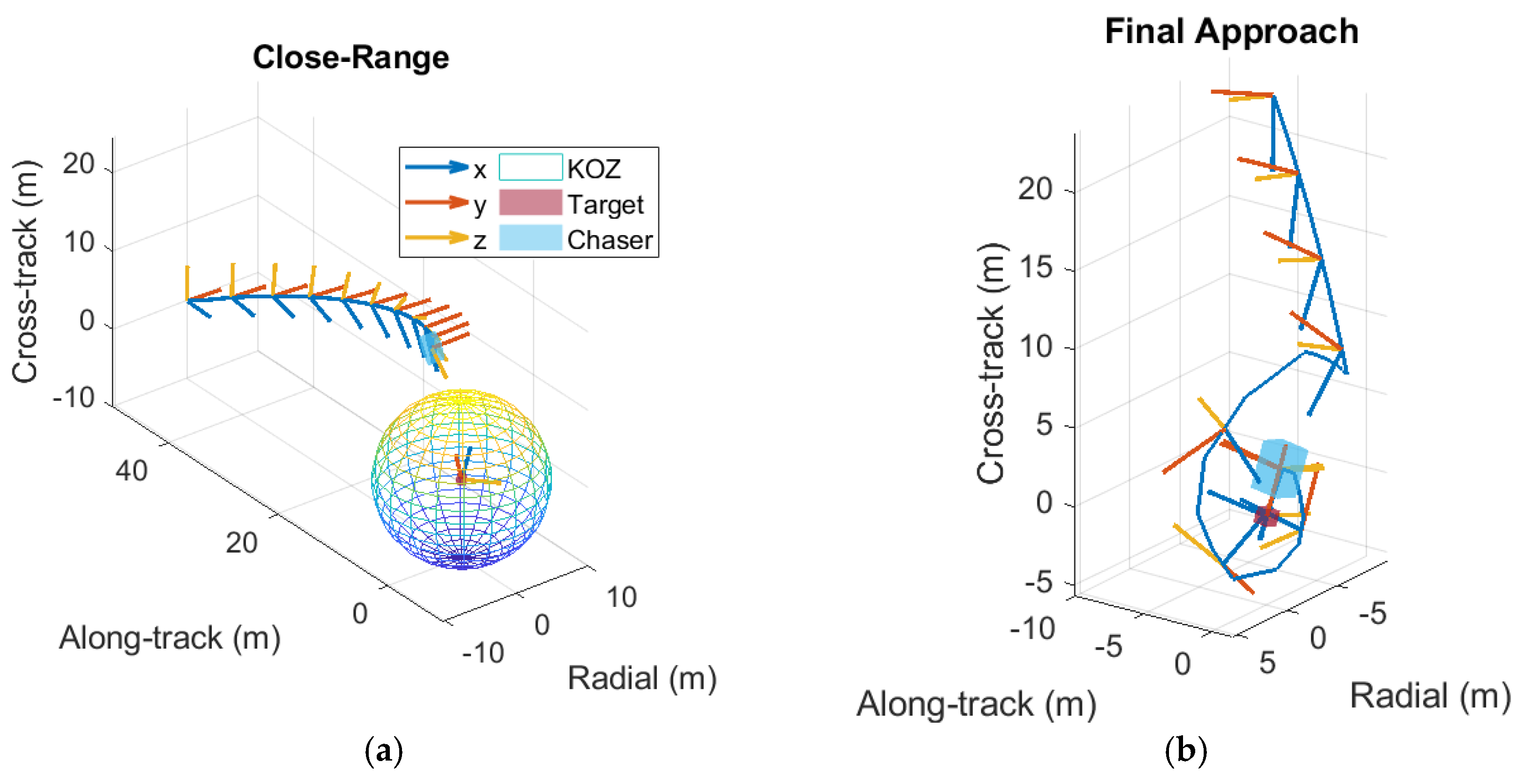
Figure 12.
The 3D planned trajectory: (a) Close-Range and (b) Final Approach phase. The x axis of the chaser also denotes the boresight axis of the LIDAR.
Figure 12.
The 3D planned trajectory: (a) Close-Range and (b) Final Approach phase. The x axis of the chaser also denotes the boresight axis of the LIDAR.
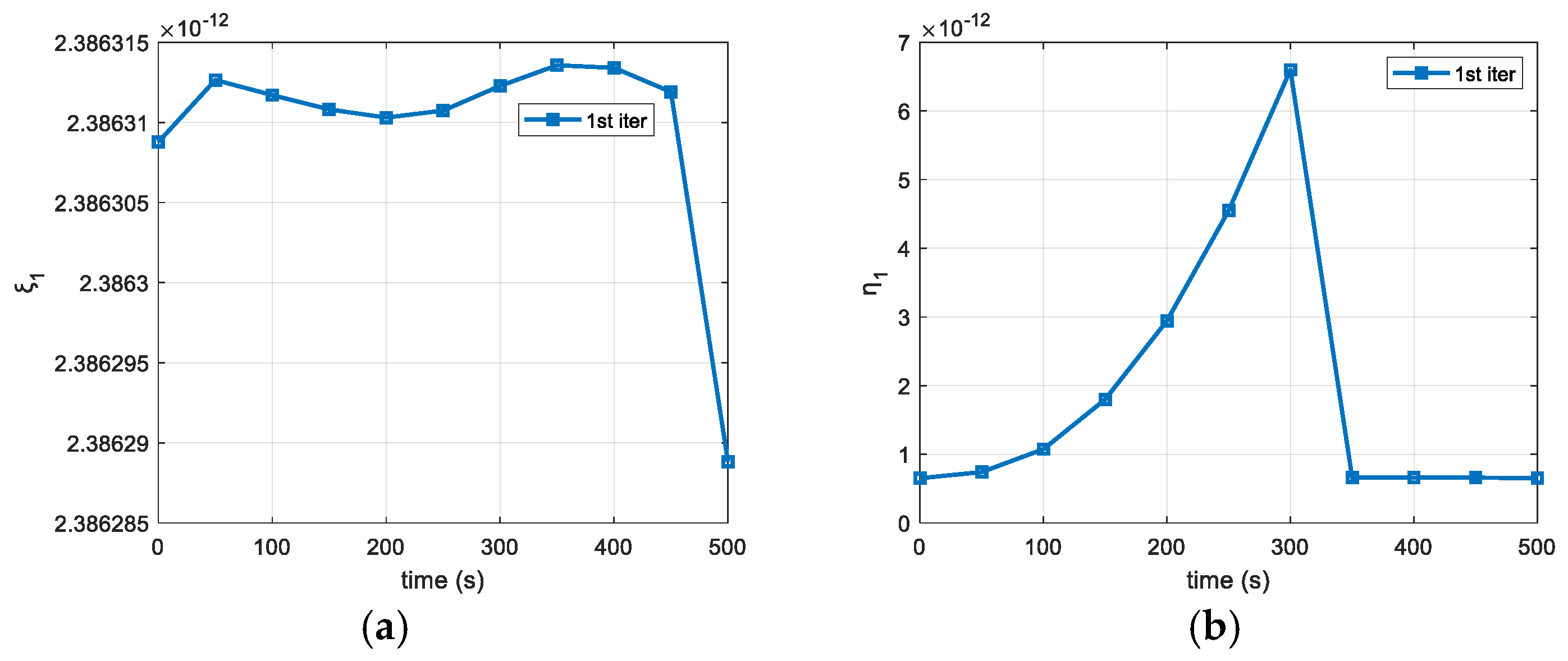
Figure 13.
(a) Trust region radius, η1, and (b) virtual buffer, ξ1 in Close-Range phase.
Figure 13.
(a) Trust region radius, η1, and (b) virtual buffer, ξ1 in Close-Range phase.
Figure 14.
(a) Trust region radius, η2, and virtual buffer, (b) ξKOZ,2 and (c) ξFOV,2 in the first segment of Final Approach phase.
Figure 14.
(a) Trust region radius, η2, and virtual buffer, (b) ξKOZ,2 and (c) ξFOV,2 in the first segment of Final Approach phase.
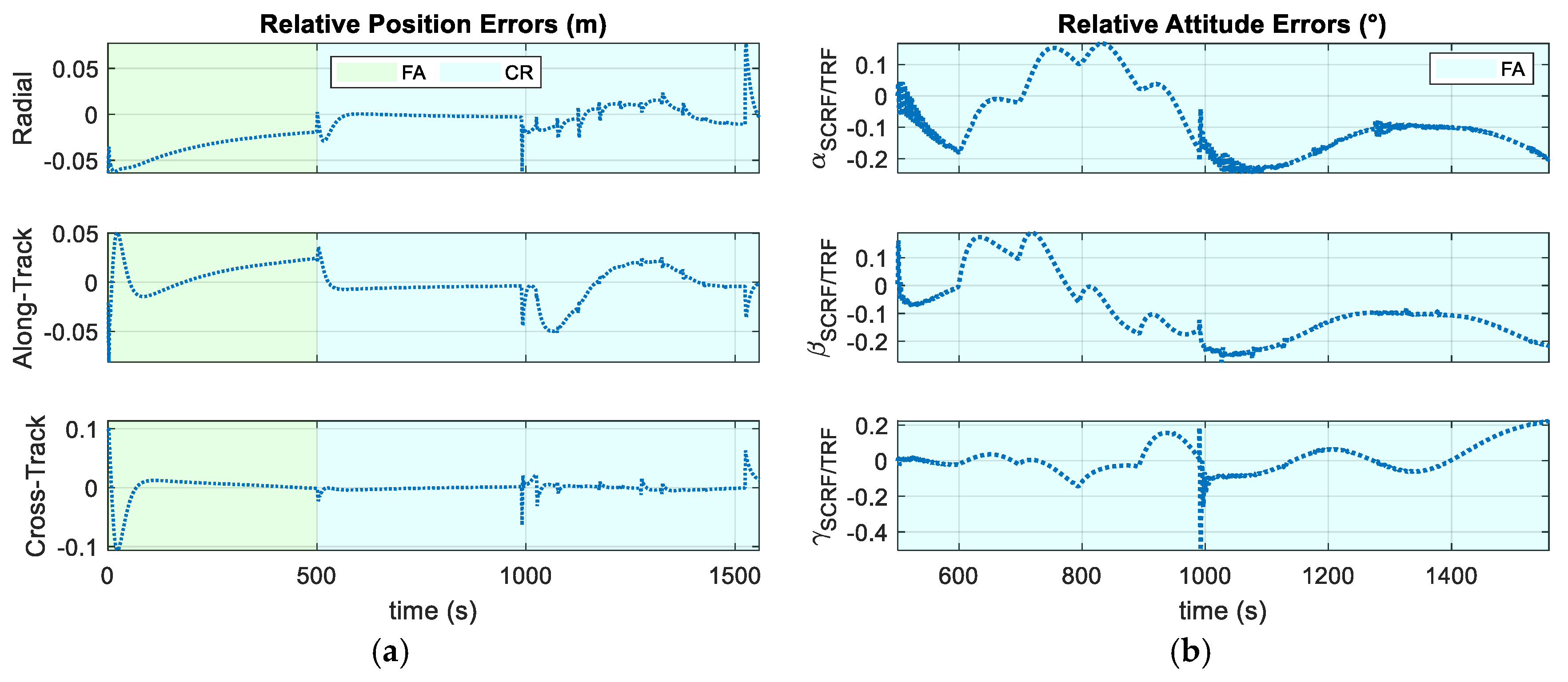
Figure 16.
Translational Control Errors: (a) Relative Position; (b) Relative Velocity.
Figure 16.
Translational Control Errors: (a) Relative Position; (b) Relative Velocity.
Figure 17.
Rotational Control Errors: (a) Equivalent Euler Angle which corresponds to the rotation quaternion δq, during the Close-Range phase; (b) Relative Attitude (3-2-1 Euler Sequence) and (c) Relative Angular Velocity during the Final Approach phase.
Figure 17.
Rotational Control Errors: (a) Equivalent Euler Angle which corresponds to the rotation quaternion δq, during the Close-Range phase; (b) Relative Attitude (3-2-1 Euler Sequence) and (c) Relative Angular Velocity during the Final Approach phase.
Figure 18.
Control Errors: (a) Relative Position; (b) Relative Attitude. The simulation is performed without the application of the dispatching function.
Figure 18.
Control Errors: (a) Relative Position; (b) Relative Attitude. The simulation is performed without the application of the dispatching function.
Figure 19.
Distribution of the Relative Position Control Errors at the end of the simulation: (a) Radial component; (b) Along-Track component; (c) Cross-Track component.
Figure 19.
Distribution of the Relative Position Control Errors at the end of the simulation: (a) Radial component; (b) Along-Track component; (c) Cross-Track component.
Figure 20.
Distribution of the Relative Velocity Control Errors at the end of the simulation: (a) Radial component; (b) Along-Track component; (c) Cross-Track component.
Figure 20.
Distribution of the Relative Velocity Control Errors at the end of the simulation: (a) Radial component; (b) Along-Track component; (c) Cross-Track component.
Figure 21.
Distribution of the Relative Attitude Errors at the end of the simulation: (3-2-1 Euler Angles): (a) αTRF/HRF; (b) βTRF/HRF; (c) γTRF/HRF.
Figure 21.
Distribution of the Relative Attitude Errors at the end of the simulation: (3-2-1 Euler Angles): (a) αTRF/HRF; (b) βTRF/HRF; (c) γTRF/HRF.
Figure 22.
Distribution of the Relative Angular Velocity Errors at the end of the simulation: (a) X SCRF component; (b) Y SCRF component; (c) Z SCRF component.
Figure 22.
Distribution of the Relative Angular Velocity Errors at the end of the simulation: (a) X SCRF component; (b) Y SCRF component; (c) Z SCRF component.
Table 1.
Parameters for numerical propagation of orbital and rotational dynamics.
Table 1.
Parameters for numerical propagation of orbital and rotational dynamics.
| Parameter | Value |
|---|
| Gravity | Model | EGM2008 |
| Maximum degree | 70 |
| Maximum order | 70 |
| Third-body perturbations | Included effects | Sun—Moon |
| Atmospheric drag | Model | NRLMSISE00 |
| Drag Coefficient | 2.0 |
| Solar radiation | Solar radiation pressure | 4.57 × 10⁻⁶ N/m2 |
| Reflective coefficient | 1.0 |
Table 6.
Chaser spacecraft characteristics.
Table 6.
Chaser spacecraft characteristics.
| Parameter | Value |
|---|
| Inertia matrix Ic (kgm2) | |
| Mass (kg) | 2000 |
| L × W × H (m) | 3 × 2 × 2 |
| FOV/2 (°) | 20 |
| Δvmax (m/s) | 0.165 |
| Δωmax (°/s) | 3.15 |
| [1 0 0]T |
| (m) | [1.5 0 0]T |
Table 7.
Target spacecraft characteristics.
Table 7.
Target spacecraft characteristics.
| Parameter | Value |
|---|
| Inertia matrix, It, (kgm2) | |
| Mass (kg) | 380 |
| L × W × H (m) | 1 × 1 × 1 |
Table 8.
Simulation characteristics.
Table 8.
Simulation characteristics.
| Parameter | Value |
|---|
| Semi-major axis (km) | 6928 |
| Eccentricity | 0.002 |
| Orbit inclination (°) | 5.20 |
| Right Ascension of the Ascending Node (°) | 0 |
| Argument of perigee (°) | 0 |
| True Anomaly (°) | 0 |
| Orbital Period (s) | 5711.8 |
Table 9.
Initial nominal conditions of the simulation.
Table 9.
Initial nominal conditions of the simulation.
| Parameter | Value |
|---|
| (m) | [0 50 0]T |
| (m) | [0 0 0]T |
| [0 0 −0.71 0.71]T |
| [0.032 0.032 −0.71 0.71]T |
| (°/s) | [0 0 0.063]T |
Table 10.
Stabilization Thresholds.
Table 10.
Stabilization Thresholds.
| Threshold | Value |
|---|
| Relative Position (m) | 0.025 |
| Relative Velocity (m/s) | 0.01 |
| Relative Attitude (°) | 2.0 |
| Relative Angular Velocity (°/s) | 0.5 |
| Stabilization Threshold Duration (s) | 30 |
Table 11.
Statistical Values of the initial conditions.
Table 11.
Statistical Values of the initial conditions.
| Uncertainties | Value (3σ) |
|---|
| Initial Misalignment of the LIDAR boresight (°) | 5 |
| Knowledge of the Initial Relative Position (cm) | 25 |
| Knowledge of the Initial Relative Velocity (cm/s) | 2 |
| Knowledge of the Chaser mass (%) | 5 |
| Knowledge of the Chaser inertia (%) | 5 |
| RCS misalignment (°) | 0.01 |
| RCS displacement (mm) | 5 |
| Knowledge of Chaser’s CoG (mm) | 5 |
| RWs misalignment (°) | 0.01 |
| RCS displacement (mm) | 5 |
| Knowledge of the target inertia (%) | 5 |
Table 12.
User-defined parameters of the guidance function including SCP implementation.
Table 12.
User-defined parameters of the guidance function including SCP implementation.
| Parameter | Value |
|---|
| d1, d2, d3 (m) | 25, 10, 3 |
| [0 1 0]T |
| (m) | [0 3 0]T |
| αcone (°) | 15 |
| KOZ radius, r1, r2, r3 (m) | 10, 10, 2 |
| t1, t3 (s) | 500, 500 |
| N1, N2, N3 | 10, 5, 10 |
| φdes (°) | 30 |
| t2,max, t2,min, t2,pred (s) | 2000, 100, 2000 |
| wη,1, wη,2, wη,3 | 500, 100, 100 |
| wξ,1, wξ,2, wξ,3 | 100, 1000, 1000 |
| εx, εJ | 5 × 10⁻⁴ |
Table 13.
Nominal Linear Velocities in Close-Range Phase.
Table 13.
Nominal Linear Velocities in Close-Range Phase.
| ΔV (cm/s) | Close Range |
|---|
| | 1st | 2nd | 3rd | 4th | 5th | 6th | 7th | 8th | 9th | 10th | 11th |
|---|
| Radial | 4.1 | 0.0 | 0.0 | 0.0 | 0.0 | 0.0 | 0.0 | 0.0 | 0.0 | 0.0 | 7.8 |
| Along-Track | −10.3 | 0.0 | 0.0 | 0.0 | 0.0 | 0.0 | 0.0 | 0.0 | 0.0 | 0.0 | 9.1 |
| Cross-Track | 3.5 | 0.0 | 0.0 | 0.0 | 0.0 | 0.0 | 0.0 | 0.0 | 0.0 | 0.0 | −4.1 |
Table 14.
Nominal Linear Velocities in Synchronization segment of Final Approach Phase.
Table 14.
Nominal Linear Velocities in Synchronization segment of Final Approach Phase.
| ΔV (cm/s) | Synchronization Phase |
|---|
| | 1st | 2nd | 3rd | 4th | 5th | 6th |
|---|
| Radial | −0.1 | 0.0 | 0.0 | 0.0 | 0.0 | 7.9 |
| Along-Track | 1.7 | 0.0 | 0.0 | 0.0 | 0.0 | −2.4 |
| Cross-Track | 2.7 | 0.0 | 0.0 | 0.0 | 0.0 | 12.2 |
Table 15.
Nominal Linear Velocities in Closing segment of Final Approach Phase.
Table 15.
Nominal Linear Velocities in Closing segment of Final Approach Phase.
| ΔV (cm/s) | Closing Phase |
|---|
| | 1st | 2nd | 3rd | 4th | 5th | 6th | 7th | 8th | 9th | 10th | 11th |
|---|
| Radial | −1.5 | −3.1 | −4.9 | −3.2 | −1.7 | −0.8 | 1.8 | 1.7 | 0.6 | 0.6 | 1.5 |
| Along-Track | 0.8 | 0.9 | 1.7 | 1.1 | 0.1 | 1.4 | −1.6 | −1.3 | −0.5 | −0.5 | −1.4 |
| Cross-Track | −7.6 | −3.1 | −0.7 | 1.9 | 1.3 | 3.7 | 3.2 | 0.0 | −0.3 | 0.0 | −0.8 |
Table 16.
Nominal Angular Velocities in Synchronization segment of Final Approach Phase.
Table 16.
Nominal Angular Velocities in Synchronization segment of Final Approach Phase.
| Δω (°/s) | Synchronization Phase |
|---|
| | 1st | 2nd | 3rd | 4th | 5th | 6th |
|---|
| X SCRF | 0.000 | −0.001 | −0.001 | −0.001 | −0.001 | 0.149 |
| Y SCRF | −0.003 | −0.006 | −0.006 | −0.006 | −0.007 | −0.127 |
| Z SCRF | 0.004 | 0.003 | 0.002 | 0.002 | 0.000 | −0.720 |
Table 17.
Comparison between the reference trajectories obtained with the two initialization methods: number of SCP iterations until convergence and propellant consumption.
Table 17.
Comparison between the reference trajectories obtained with the two initialization methods: number of SCP iterations until convergence and propellant consumption.
| Maneuver Phase | Initial Guess Methodology |
|---|
| | Semi-Analytical Approach | Polynomial Interpolation |
|---|
| Iterations | (cm/s) | Iterations | (cm/s) |
|---|
| Close-Range | 1 | 24.3 | 3 | 35.3 |
| Synchronization | 2 | 17.9 | 2 | 18.6 |
| Closing | 19 | 37.8 | 50 | 54.0 |
Table 18.
Parameters A1,i, M1,i, ω1,i, A2,i, M2,i, ω2,i, A3,i, M3,i, and ω3,i (Translational H infinity Controller).
Table 18.
Parameters A1,i, M1,i, ω1,i, A2,i, M2,i, ω2,i, A3,i, M3,i, and ω3,i (Translational H infinity Controller).
|
Weights
|
Value
|
Weights
|
Value
|
Weights
|
Value
|
|---|
| A1,i | 0.01 | A2,i | 1000 | A3,i | 0.05 |
| M1,i | 1.8 | M2,i | 10 | M3,i | 10 |
ω1,i
(rad/s) | 0.01 | ω2,i
(rad/s) | 0.05 | ω3,i
(rad/s) | 0.05 |
Table 19.
Parameters A1,i, M1,i, ω1,i, A2,i, M2,i, ω2,i, A3,i, M3,i, and ω3,i (Roto-translational H infinity Controller).
Table 19.
Parameters A1,i, M1,i, ω1,i, A2,i, M2,i, ω2,i, A3,i, M3,i, and ω3,i (Roto-translational H infinity Controller).
| Weights | Value | Weights | Value | Weights | Value |
|---|
| A1,i | 0.01 | A2,i i = 1, …, 6 | 100 | A3,i | 0.01 |
| A2,i i = 7, …, 12 | 1000 |
| M1,i | 1.8 | M2,i | 10 | M3,i | 10 |
ω1,i
(rad/s) | 0.04 | ω2,i
(rad/s) | 0.40 | ω3,i
(rad/s) | 0.40 |
Table 20.
Standard deviation (σ), mean value (μ) and maximum value (Max) of the Relative Position and Attitude Control errors over the entire simulation.
Table 20.
Standard deviation (σ), mean value (μ) and maximum value (Max) of the Relative Position and Attitude Control errors over the entire simulation.
| Position | σ | μ | Max | Attitude | σ | μ | Max |
|---|
| Radial (cm) | 4.0 | −1.6 | 33.8 | αSCRF/TRF (°) | 0.39 | −0.15 | 1.30 |
| Along-Track (cm) | 4.8 | −0.1 | 35.8 | βSCRF/TRF (°) | 0.35 | −0.11 | 1.12 |
| Cross-Track (cm) | 4.7 | −0.4 | 48.0 | γSCRF/TRF (°) | 0.38 | 0.10 | 1.51 |
Table 21.
Standard deviation (σ), mean value (μ) and maximum value (Max) of the Relative Position and Attitude Control errors over the entire simulation in the idea case.
Table 21.
Standard deviation (σ), mean value (μ) and maximum value (Max) of the Relative Position and Attitude Control errors over the entire simulation in the idea case.
| Position | σ | μ | Max | Attitude | σ | μ | Max |
|---|
| Radial (cm) | 1.9 | −1.2 | 7.7 | αSCRF/TRF (°) | 0.11 | −0.08 | 0.25 |
| Along-Track (cm) | 1.7 | 0.0 | 8.1 | βSCRF/TRF (°) | 0.12 | −0.09 | 0.27 |
| Cross-Track (cm) | 1.5 | 0.0 | 11.0 | γSCRF/TRF (°) | 0.08 | 0.01 | 0.50 |
Table 22.
Comparison of 1-norm of the commanded force components computed by the H infinity controller in the two scenarios.
Table 22.
Comparison of 1-norm of the commanded force components computed by the H infinity controller in the two scenarios.
| Realistic Actuators | Impulsive Actuators |
|---|
| Component | Value | Component | Value |
|---|
| X SCRF (N) | 13,752.9 | X SCRF (N) | 7858.8 |
| Y SCRF (N) | 5154.0 | Y SCRF (N) | 4521.6 |
| Z SCRF (N) | 9476.0 | Z SCRF (N) | 2655.9 |
