Abstract
Based on the analysis of solar array current data from a certain MEO-orbiting satellite, this paper reveals its short-period fluctuation characteristics and underlying mechanisms. The study finds that when solar panels face the sun during the light period, the output current exhibits significant short-period fluctuations in addition to being influenced by long-period factors such as sun–earth distance, incident light intensity changes, and space irradiation attenuation. Through theoretical analysis, we first confirm that the root cause of these short-period variations is the temperature change in the shunt circuit caused by load fluctuations, which in turn affects the output current characteristics. Unlike traditional methods that use static characteristic factors such as incident angles, this paper innovatively proposes using load current as a key characteristic factor. For asymmetric solar panel fault scenarios, load current, time phase, and fault-wing output current are used as characteristic factors to adaptively predict the current of normal wings. Meanwhile, feedforward neural network (FNN), Recurrent Neural Network (RNN), and long short-term memory (LSTM) are used for output current prediction. The experimental results show that these methods can accurately capture the short-period fluctuations caused by load mutations and adapt to the fluctuation trend of the normal wing during the prediction of current changes in the faulty wing. It is worth noting that, limited by the short-period fluctuation prediction scenario, the inherent advantage of LSTM in long-sequence prediction is not fully reflected.
1. Introduction
As a core component of the satellite energy system, the stability of the output power of the spacecraft solar array directly determines the reliability of the satellite’s on-orbit mission [1]. Factors affecting the output current of the Solar Array include temperature, solar irradiance, solar incidence angle, space particle radiation, local shadow, and solar panel drive faults [2,3,4]. Most studies focus on long-term degradation (such as sun–earth distance factors, solar incidence angle, irradiance, irradiation, etc.).
Zhang Yong et al. considered factors such as solar incidence angle, sun–earth distance, operating temperature, and space environment [5,6]. Jing et al. considered the influence of factors such as earthshine and satellite module occlusion (based only on satellite configuration) [7]. Xiong et al. comprehensively analyzed key variables, including earthshine, satellite module occlusion, satellite attitude deviation, solar cell operating temperature, and space environment [8]. Yu et al. proposed a simplified performance degradation model to analyze the long-term characteristics of solar array output current [9]. Li Qiang et al. predicted array degradation under the premise of normalizing the illumination angle and power temperature coefficient [10]; Liao et al. established a theoretical model including solar radiation, shadow, thermal characteristics, and output power for the problem of solar array shadowing by balloons in stratospheric balloons [11]. Mokhtar et al. proposed a modeling environment for low-earth orbit (LEO) spacecraft solar arrays (SSA), constructing a mathematical model including irradiance, temperature, and energy balance [12]. Saravanan et al. considered power loss under shadow conditions [13].
In recent years, machine learning and deep learning technologies have shown significant potential in the field of energy forecasting. For example, scholars such as Sunori achieved high-precision prediction of solar panel power output based on artificial neural network (ANN) and random forest (RF) models [14]; Chen et al. confirmed the effectiveness of current features in anomaly detection of satellite solar arrays through standardized diagnostic methods [15]. However, most existing studies focus on long-term steady-state forecasting, with insufficient adaptability to model short-term fluctuations. Although random forests have the ability to analyze feature importance, they have limitations in modeling temporal dependencies [16]; while autoregressive integrated moving average models (ARIMA) are suitable for linear time series forecasting, they struggle to capture dynamic nonlinear fluctuations [17].
Traditional prediction models mostly rely on environmental parameters (such as temperature and irradiance). For example, Yan et al. used BP neural networks to predict solar array current, but the prediction error was large (0.1 A) due to the lack of consideration of the temporal characteristics of load current [18]; another study by Zuo et al. reported an average relative error of 3% in predicting the long-term degradation of solar arrays [19].
In contrast, as the basic model of neural networks, FFN (Feedforward Neural Network) realizes complex function approximation through multi-layer nonlinear transformations; RNN (Recurrent Neural Network) enables the model to capture the temporal dependency in sequences by introducing a “recurrent” structure; Long Short-Term Memory (LSTM) stands out in capturing long-term dependencies in time series by virtue of its gating mechanism [20]. These neural network models provide new paths for the short-period fluctuation prediction of solar array current.
Cao Xinyue et al. analyzed the thermoelectric coupling under parallel mismatch of triple-junction GaAs solar cells for satellites and provided suggestions for the series-parallel design of arrays to prevent parallel mismatch [21]. However, they did not analyze the small-amplitude fluctuations in the output current of the battery array under thermoelectric coupling conditions.
Song et al. [22] proposed a new hybrid deep learning method that integrates the complementary advantages of Recurrent Neural Networks (RNNs), Transformer models, and Long Short-Term Memory (LSTM) networks, aiming to improve the accuracy of solar energy prediction. By combining serial processing with a multi-head self-attention mechanism, this model can capture complex dependencies across different time scales, thereby enhancing the performance of time series prediction. It is worth noting that this study did not include load current as a feature factor; instead, it focused on modeling relevant influencing factors such as weather conditions. The model was validated through experiments under diverse and complex weather scenarios, including sunny, cloudy, and rainy days.
From the above survey, it can be seen that current research lacks a systematic analysis of the short-term current fluctuation characteristics of load-fluctuating satellites (such as communication satellites, reconnaissance satellites, navigation satellites, etc.). When the satellite load current changes according to a certain transmission–reception time slot due to mission modes (such as antenna transmission–reception switching), the array output current exhibits obvious short-term fluctuations, especially under asymmetric panel configurations (such as one-wing faults). In short-term scenarios, the dynamic response of the solar array is significantly affected by changes in load current. As a core characteristic factor reflecting external demand and system dynamic response, the potential value of load current has not been fully exploited. Although existing studies have shown that feature selection is crucial for model accuracy [23], there is still a lack of systematic research on the temporal characteristics and nonlinear correlations of load current in short-term fluctuation forecasting, requiring methodological innovation.
To address the above challenges, this paper first elaborates on the dynamic compensation mechanism of shunt regulation in the design of the Main Error Amplifier (MEA) based on the topological structure of the satellite power supply system S3R (Sequential Switching Shunt Regulator). Through Pearson correlation coefficient analysis, feature factors are screened, excluding temperature and MEA parameters, and retaining load with clearer physical meaning as the key factor for short-term prediction of solar array current.
This paper constructs a multi-algorithm comparison framework based on load current and time phase, aiming to reveal the internal correlation between them and the output fluctuations of solar arrays. The three constructed neural network models can control the root mean square error (RMSE) within 0.05 A. Ground operation and maintenance can design dynamic threshold alarm strategies based on the prediction results.
2. Overview of Shunt Regulation Design for Satellite Power Supply Systems
The power system of a certain MEO orbit satellite consists of a solar array, a lithium-ion battery pack, a power controller, etc. The main function of the power subsystem is to realize the energy transfer and power balance between the solar array and the battery pack, ensuring the normal power supply of the primary power system [24,25,26,27].
The power controller adopts a three-domain full-regulation control bus scheme using a voltage error signal. The MEA uniformly manages the power regulation modules inside the power controller to keep the bus voltage constant, whether in the light period or the shadow period [28,29,30].
The main function of the MEA error amplifier is to collect the 42 V bus voltage, compare it with a set reference value after transformation to generate an MEA control signal, and then send it to the shunt circuit through a two-out-of-three voting circuit to stabilize the primary bus. The principle block diagram is shown in Figure 1 [31,32,33].
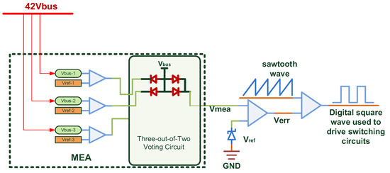
Figure 1.
Principal block diagram of main error amplifier (MEA).
The bus error signal can be expressed by Equation (1).
: Bus error signal; : Amplifier gain; : Bus voltage; : Circuit voltage reference. K represents the voltage division factor.
The shunt regulator of the power controller is used for power regulation of the solar array during the light period [34]. The entire shunt regulator consists of 12 identical shunt circuits, each with a single-stage shunt capacity of 7 A. When the system is balanced, only one of the 12 shunt circuits is in the adjustment state, while the others are in the cutoff or conduction state. During the light period, the solar array current is constant. When the load decreases, the bus voltage increases, the MEA voltage rises, and the 12 shunt circuits sequentially enter the shunt state; conversely, when the load increases, the bus voltage decreases, the MEA voltage drops, and the shunt circuits sequentially exit the shunt state. The solar cell circuits are shorted to ground or supply power to the bus according to the load demand, maintaining the stability of the bus voltage by regulating the supply current of the solar array [35,36,37,38].
The circuit reference of the shunt circuits is formed by a series-connected resistor network. All shunt circuits correspond to 12 voltage references in total, with the lowest voltage corresponding to the first-stage shunt circuit. The threshold voltage data for each stage of the shunt regulator, obtained through experiments, are shown in Table 1 below. By referring to Table 1 and combining it with the actual measured VMEAS3R data, the real-time status of each shunt circuit in the shunt regulator can be determined.

Table 1.
Measured data table of shunt circuit stages and corresponding shunt threshold voltages.
In response to the 12-stage shunt operation mode of the PCU, the solar array is designed with 12 sub-arrays in total. Sub-arrays 1–12 sequentially correspond to the controller’s 1–12 shunt stages. Each wing contains six sub-arrays: the +Y wing houses sub-arrays 1, 3, 5, 7, 9, and 11; the −Y wing houses sub-arrays 2, 4, 6, 8, 10, and 12.
The distribution of thermistors on the +Y wing of the solar array is as follows: Thermistor 1 is located in the first-stage shunt circuit (PC1, inner panel), Thermistor 2 in the seventh-stage shunt circuit (PC9, inner panel), and Thermistor 3 in the fifth-stage shunt circuit (PC7, outer panel). For the −Y wing of the solar array, the thermistor distribution is Thermistor 1 in the first-stage shunt circuit (PC2, inner panel), Thermistor 2 in the seventh-stage shunt circuit (PC10, inner panel), and Thermistor 3 in the fifth-stage shunt circuit (PC8, outer panel).
Whether the circuit at the temperature measurement point is shunting is controlled by the shunt regulator (S3R). When a specific S3R shunt regulation circuit is in the shunt state, the thermistor at the temperature measurement point of that circuit generates heat, causing the corresponding thermistor telemetry temperature to rise. When a specific S3R shunt regulation circuit is in the cut-off state, the corresponding thermistor telemetry temperature decreases.
The principal block diagram of the shunt regulation circuit is shown in Figure 2 below.
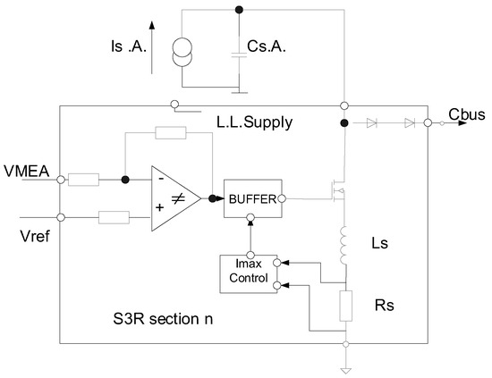
Figure 2.
Principal block diagram of the shunt regulation circuit.
From the principle of the shunt circuit, it is known that the temperature of the battery array when supplying the load is lower than that when shunting, and shunting generates heat dissipation in the diode.
3. Description of Problem Phenomenon and Theoretical Analysis
3.1. Description of Phenomenon 1
A certain MEO orbit satellite exhibits small-amplitude fluctuations in solar array current over a short period, which is particularly evident during high-power switching operations of payloads, leading to significant changes in load current (with an amplitude of approximately 28.89 A). When the satellite performs high-power switching, drastic changes in load current trigger voltage fluctuations in the Main Error Amplifier (MEA) of the power supply system and adjustments in the number of shunt stages. The specific changes in telemetry data are shown in Figure 3 and Figure 4 below.
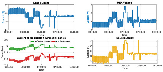
Figure 3.
Trend diagram of load, solar array current, shunt current, and MEA.
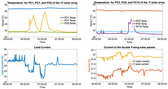
Figure 4.
Trend diagram of solar array shunt stage temperature and load current.
3.2. Analysis of the Causes of Phenomenon 1
When the load current decreases from 45 A to 20 A, the 7th–8th shunt stages switch from load supply to shunt mode, causing the temperature to rise from 35 °C to 47 °C. Along with the adjustment of the shunt stages, fluctuations in MEA voltage occur (from approximately 16 V to 18 V). By comparing the data in Table 1, it can be seen that the 7th–8th stages change from the load supply mode to the shunt mode. It reflects the dynamic power distribution changes in the power supply system. The 1st–2nd stages continuously shunt, while the 9th–10th stages continuously supply the load, with both showing slight temperature fluctuations. The decrease in load current leads to a rise of approximately 0.1 A in the solar array current, which is directly related to the operational state transition of the 7th–8th stages, demonstrating the thermal–electrical coupling effect caused by power distribution adjustments.
Due to the presence of a transmitting antenna, the satellite performs signal transmission and reception operations according to a scheduled routing plan. During routine on-orbit operation, the power in the transmission phase is higher than that in the reception phase, causing the load current to fluctuate slightly within a certain range, with an amplitude smaller than that during high-power single-unit switching. Therefore, in normal operation mode, the load current of the satellite changes within a specific range, and accordingly, the output current of the corresponding solar array also exhibits slight range fluctuations.
3.3. Description of Phenomenon 2
A stall occurred in the negative Y drive of a certain satellite, causing the output current of its positive Y wing to exhibit increased short-period fluctuation amplitude compared to before the stall.
On March 6, the negative Y SADM (Solar Array Drive Mechanism) stopped rotating, the current of the negative −Y wing solar panel showed periodic changes between 0 and the maximum value. At the same time, the current of the positive −Y solar panel changed from the previous short-period fluctuation of 0.2 A to two sinusoidal fluctuations with an amplitude of about 0.5 A within a day. The fluctuation period and direction are consistent with those of the negative−Y. The details are shown in Figure 5 and Figure 6 below.
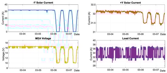
Figure 5.
Trend diagram of load, solar array current, and MEA for Satellite B.
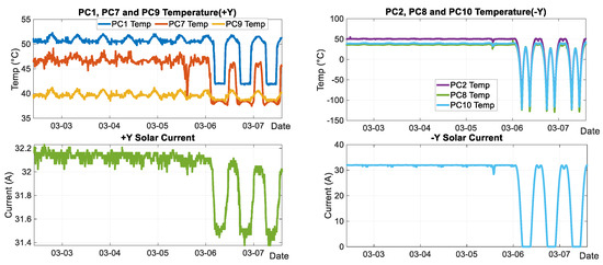
Figure 6.
Trend diagram of solar array shunt stage temperature and load current for Satellite B.
3.4. Analysis of the Causes of Phenomenon 2
The logical chain of causes for the phenomenon in the above figure is as follows:
- Negative Y-wing current decreases → Positive Y-wing power supply mode switches → Shunt stage temperature changes → Output current fluctuates → Total current responsiveness changes;
- Changes in illumination conditions → Synergetic changes in Negative Y-wing current and temperature → Extremely low temperature without illumination.
The specific elaboration is as follows:
As shown in the figure, under normal conditions, the satellite load current stabilizes in the range of 29 A–37 A, and the normal solar array current of both wings fluctuates around 32 A. When the Negative Y-wing solar array current drops from the maximum value of 32 A to the minimum value (approximately 0 A), the Positive Y-wing power supply mode switches from “stages 12-9 supplying the load, stage 8 adjusting (MEA 16.65 V)” to “stages 12-1 supplying the load (MEA 10 V)”. The temperature rises when the shunt circuit shunts to ground and decreases when supplying the load. For stages 1, 3, 5, and 7 of the +Y wing transition from the shunt state to the load supply state, causing a temperature decrease. This temperature reduction subsequently leads to a decline in the output current of the corresponding shunt levels, ultimately resulting in a decrease in the total current of the +Y wing. Stage 9 of the +Y wing remains in the load supply state, with no significant temperature change.
The Negative Y-wing solar array current decreases as the solar incidence angle increases, and the reduction in the light intensity factor causes the output current of a single sub-array to drop. The illumination factor decreases synchronously, and the temperature change trend is consistent with the Negative Y-wing current; the temperature can drop to −120 °C without illumination. When the Negative Y-wing solar array current recovers from the minimum value to the maximum value, the shunt circuits of the Positive Y-wing sequentially re-enter the shunt state, the temperature gradually rises, and the total current recovers accordingly.
3.5. Theoretical Calculation
Taking the MEO orbiting satellite described in Phenomena 1 and 2 as an example, the parameter table of the satellite’s solar cells is shown in Table 2.
Table 2.
Electrical parameters table of solar cells.
The design parameters of the solar cell circuit for this satellite are shown in Table 3 below:
Table 3.
The relevant parameter table adopted for the design of the solar cell circuit.
The satellite has 12 sub-arrays, with each sub-array consisting of 16 cells in parallel. Theoretically, based on the number of parallel single-cell panels in each sub-array and temperature changes, the variation in the output current of the entire wing under such conditions can be analyzed.
According to on-orbit data, when a sub-array is in the shunt state, the average temperature of the array is about 53 °C; when the sub-array is in the power supply state, the average temperature of the array is about 38 °C.
According to Formula (2):
In the formula:
: Optimum operating point current of a single solar cell at the beginning of life (17.13 mA/cm2);
: Area of the solar cell (39.8 mm × 60.4 mm);
: Current temperature coefficient (0.014 mA/cm2 °C);
T: Operating temperature for current;
: Current ultraviolet radiation loss factor (0.91);
: Current combination loss factor (0.98);
: Current particle irradiation degradation factor (0.98).
Through calculation, the changed current is (53 − 38) × 4 × 6 × 0.010 × 16 × 8 = 460.8 mA, which is basically consistent with the actual fluctuation of 0.5 A. The reasons for the difference are as follows: first, the selection difference in the current coefficient βᵢ; second, the number of working state adjustments of the eight sub-arrays is different from the theoretical situation (a certain circuit is in the adjustment state with a certain duty cycle). At the same time, the sun–earth distance factor will also affect the results.
Due to the change in the solar angle, the current intensity of the solar panel on the negative Y-wing changes, and the temperatures of the three thermistors all change significantly, with the fluctuation trend consistent with the current of the negative Y-wing solar panel.
4. Materials and Methods
Although theoretical calculations in the previous chapter can estimate the amplitude of solar array current variations, satellite resource limitations mean that not every sub-array is equipped with temperature telemetry. As a result, it is challenging to calculate total current changes using only theoretical methods. Instead, algorithms can be employed to derive these variations and serve as a basis for determining whether the solar array current is operating normally.
This section establishes a prediction model for solar array output fluctuations by leveraging load current as the core short-period characteristic factor. Through comparative analysis of the predictive performance of LSTM, Recurrent Neural Network (RNN), ARIMA, and Feedforward Neural Network (FFN), the suitability of different algorithms for short-period time-series modeling is systematically evaluated. Experimental results show that both LSTM and RNN models can effectively capture the dynamic nonlinear relationship between load current and battery array output, with prediction accuracy superior to other comparative algorithms. However, LSTM has no significant advantage over RNN and has the problem of increasing resource occupation.
4.1. Introduction to the LSTM Algorithm
The Long Short-Term Memory Network (LSTM), an improved variant of the Recurrent Neural Network (RNN), is specifically designed to address the gradient vanishing/exploding issues faced by traditional RNNs when processing long-sequence data, enabling effective capture of long-range dependencies. Its core idea lies in introducing a gating mechanism to selectively control information flow, thus achieving storage and management of long-term memory [39,40,41].
An LSTM consists of a cell state () and three gating units: the forget gate, input gate, and output gate. Each gating unit uses a sigmoid activation function to output values between 0 and 1, representing the proportion of information allowed to pass through [42].
The LSTM model designed in this paper employs a two-layer network structure with the following specific configurations:
- The first layer adopts a unidirectional LSTM structure with 64 memory units, returning full sequence outputs;
- The second layer contains 32 memory units, returning only the output of the last time step in the sequence;
- A 30% Dropout layer is set after each LSTM layer to suppress overfitting;
- The output layer uses a fully connected structure with a Relu activation function for nonlinear transformation;
For model training:
- The Adam optimizer is used to adaptively adjust the learning rate;
- The Huber loss function is selected (with stronger robustness to outliers);
- An early stopping mechanism is applied, halting training when validation loss shows no improvement for 10 consecutive epochs;
- A learning rate adjustment strategy is adopted: if validation loss remains unchanged for 5 consecutive epochs, the learning rate is reduced by 80%.
This combination of network structure and training strategies effectively captures dependencies in time series while ensuring the model’s generalization ability and training stability [43]. The schematic diagram of LSTM is shown in Figure 7 below [44].
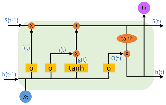
Figure 7.
Schematic diagram of LSTM.
Taking the first layer of the model as an example, the specific calculation process is as follows:
Forget Gate Stage: The forget gate calculates its output using the formula ( denotes the Sigmoid function), based on the current input and the previous hidden state . This output is element-wise multiplied by the previous cell state to determine which information to discard from .
Memory Update Stage: The Sigmoid component of the input gate computes the proportion of information to update via . The tanh component generates a candidate vector . The cell state is updated as .
Output Stage: The output gate first determines the output proportion through . The final output is then computed as , which serves as the input for the next time step or the model’s prediction.
For the first LSTM layer in this study:
Number of memory units: 64;
Input vector: ;
Previous hidden state: ;
Input weight matrix: ;
Hidden state weight matrix: ;
Bias vector: .
Thus, the formula for the forget gate in the first LSTM layer is derived as follows:
To enhance the robustness of the code, this paper selects the Huber Loss as the loss function. The Huber Loss is a loss function that is insensitive to outliers, combining the advantages of MSE (Mean Squared Error) and MAE (Mean Absolute Error). In regression problems, it not only maintains the smoothness of MSE but also reduces the influence of outliers. For the predicted value and the true value y, the Huber Loss is defined as
where is a hyperparameter controlling the threshold at which the loss function transitions from MSE to MAE. When the error is small, MSE is used to ensure gradient smoothness; when the error is large, MAE is used to mitigate the impact of outliers. This function is continuous and differentiable at , ensuring the stability of the optimization process.
The backpropagation through time (BPTT) of LSTM requires computing the gradients of the loss with respect to each parameter. The core steps include the following:
Gradient of the output layer:
Gradient of the output gate:
Gradient of the cell state:
Gradient of the forget gate:
Gradient of the input gate:
Gradient of the candidate cell state:
The Adam optimizer used in this paper updates gradients in the following steps (taking the iteration as an example):
- 1.
- Compute the current gradient:
, which is the gradient of the loss function with respect to parameter
- 2.
- Update the first moment and second moment :
Exponential moving average update:
where and are hyperparameters (, , controlling the decay rate of historical information.
- 3.
- Bias correction (to address initialization bias):
Since and , and in the early iterations are biased toward zero. Corrections are applied as
where and are bias correction factors that diminish as the iteration count t increases.
- 4.
- Update the parameter :
Combine the first moment, second moment, and learning rate to compute the parameter update:
where is a small value to prevent division by zero.
To prevent overfitting, this paper designs callback functions including the following:
Early Stopping Mechanism: training halts when the monitored validation loss metric shows no improvement over 10 consecutive epochs, preventing overfitting and restoring the model weights with the best validation performance;
Reduce LR On Plateau: automatically reduces the learning rate when a metric has stopped improving, helping the model escape local minima and converge to a global optimum.
4.2. Introduction to RNN Algorithm
A Recurrent Neural Network (RNN) is a class of neural networks specifically designed to process sequential data. By introducing a “recurrent” structure, the model can capture temporal dependencies in sequences. Its core characteristics are as follows:
Parameter Sharing: The same weight matrices are used across different time steps, reducing model complexity.
Memory Mechanism: Historical information is transmitted through hidden states to model the context of sequences.
The update formula for the hidden state of an RNN is
where is the input at time step t; is the hidden state from the previous time step (with an initial value as a zero vector); and are shared weight matrices; denotes an activation function.
4.3. Introduction to FFN Algorithm
The Feedforward Neural Network (FFN), as the fundamental architecture of neural networks, is also known as the Multilayer Perceptron (MLP). Its characteristics include:
Unidirectional information flow: Data travels from the input layer to the hidden layers and then to the output layer without feedback connections.
Fully connected layers: Neurons in adjacent layers are all interconnected, while neurons within the same layer have no connections.
Nonlinear transformation: Nonlinearity is introduced through activation functions to enhance the model’s representational capability.
For the neuron in the layer, its output is calculated as
where is the output of the i-th neuron in the previous layer; is the connection weight; is the bias term; is the activation function.
4.4. Comparison of LSTM, RNN, and FFN Algorithms
A comparison of the three algorithms is shown in Table 4 below:
Table 4.
Comparison of three algorithms.
In this paper, the code frameworks for the three models are identical in their core components: data preprocessing logic, training loop structure (including forward propagation, loss computation, and backpropagation), and optimizer configuration.
The architectures of the three models constructed in this paper are shown in Table 5 below:
Table 5.
Summary table of training model architectures.
The training and optimization parameters of the three models are shown in Table 6 below:
Table 6.
Statistical table of model training and optimization parameters.
4.5. Introduction to ARIMA Algorithm
ARIMA (AutoRegressive Integrated Moving Average) is a classic time series forecasting method, widely used in time series data analysis and prediction in fields such as economics, meteorology, and engineering. It captures the dynamic patterns of time series by combining three mechanisms: AutoRegression (AR), Integration (I), and Moving Average (MA) [45].
The complete representation of an ARIMA model is ARIMA(p, d, q), where the three parameters correspond to the three core components of the model. It is more suitable for capturing linear dependencies and has limited performance for nonlinear sequences with sharp changes.
p: The number of autoregressive terms (AutoRegressive), representing the linear dependence of the current value on the values of the past p time steps.
d: The order of differencing (Integrated), which makes the original sequence stationary by differencing it d times (a prerequisite for time series forecasting).
q: The number of moving average terms (Moving Average), representing the linear dependence of the current value on the error terms of the past q time steps.
The default value of the parameter d in the function is 0 (indicating the assumption that the original sequence is stationary). First, an ADF stationarity test is performed on the original sequence. If the sequence is non-stationary (p-value > 0.05), a 1st-order differencing is applied (d = 1), and the stationarity is tested again. If the sequence remains non-stationary after 1st-order differencing, a 2nd-order differencing is performed (d = 2).
The ARIMA algorithm described in this paper uses the initial parameter ARIMA(2, d, 1) (where p = 2, d is determined according to the differencing order, and q = 1).
The model is fitted based on the training set data, and parameters are optimized by minimizing the AIC (Akaike Information Criterion).
4.6. Feature Factor Selection
Based on the previous phenomenon description and analysis, the factors influencing short-period characteristics include temperature, load current, and MEA. The Pearson Correlation Coefficient is used to analyze the correlation of each factor. This coefficient measures the linear correlation degree between two variables, with values ranging from [−1, 1]. A value of 1 indicates a perfect positive correlation, −1 indicates a perfect negative correlation, and 0 indicates no linear correlation. The following are its calculation formula and related explanations:
Assume two variables X and Y with a sample size of n, and their corresponding observation values are . The Pearson correlation coefficient r is calculated as
The correlation results between each factor are shown in Table 7 below:
Table 7.
Correlation analysis results.
From the above table, the following conclusion can be drawn:
For satellites with normal solar array drives, the following applies:
- Temperature exhibits low correlation with short-period characteristics and can be excluded.
- Although the MEA parameter shows high correlation with the short-period characteristics of solar array current, it is also highly correlated with load current. Considering that load current is directly linked to the short-period fluctuations of solar array current (|r| = 0.88) with a clearer physical meaning, this feature is retained while the MEA parameter is excluded to avoid information redundancy.
For satellites with single-wing solar array failures [46]:
- Time-phase factors reflecting the orbital period characteristics of the faulty wing’s output current must be retained. The “time phase” reflecting orbital periodicity is derived from raw telemetry timestamps, with integration of time intervals to capture orbital periodicity. Specifically, instead of using sine/cosine transformations of orbital angles or discrete bin indices, we directly compute the time difference (Δt) between each telemetry point and the initial telemetry point (i.e., the first sampled telemetry point) is calculated directly based on the original timestamps. This Δt is used as a core input feature; as domestic and overseas telemetry adopt 1 s and 60 s intervals, respectively, we avoid interpolation or resampling. Instead, the Δt values are fed directly into the model as a feature, allowing the algorithm to learn the impact of sampling frequency differences on current output.
- Since MEA is highly correlated with the −Y wing output current, only the −Y wing output current is retained to avoid information redundancy.
- Additionally, although temperature-related parameters (PC1, PC2, PC7, PC8) are highly correlated with the +Y wing output current prediction, their correlation with the −Y wing load current is equally significant, so temperature factors are excluded.
Regarding the exclusion of MEA as a feature factor, we conducted an experiment. We incorporated both load current and MEA voltage as feature factors in the LSTM model for Satellite A, and compared its performance with the model using only load current. The differences were quantified using three metrics: RMSE, MSE, and MAE (see specific data in Table 8). The experimental results showed that the prediction accuracies of the two feature combinations are generally comparable, while the model including MEA voltage slightly underperformed the model using only load current in all metrics. These results indicate that although MEA voltage exhibits a high Pearson correlation with the solar array output current, the information it contains can be indirectly reflected through the load current (because the MEA voltage also has an extremely high correlation with the load current). Moreover, the additional inclusion of MEA may slightly reduce the model’s generalization ability due to feature redundancy or noise interference.
Table 8.
Comparison of LSTM prediction with and without MEA as a feature factor on Satellite A.
The results of LSTM prediction for solar arrays using load current and MEA as characteristic factors are shown in Figure 8 below.
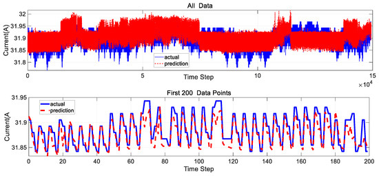
Figure 8.
Results of LSTM prediction for solar arrays using load current and MEA as feature factors.
Through this ablation experiment, we further confirmed that in short-period prediction scenarios, load current, as a core feature, can already capture the dynamic fluctuation characteristics of the solar array output current, and its sole use is sufficient to meet the requirements of prediction accuracy.
The final feature sets are determined as follows:
Normal satellites: ;
Faulty satellites: .
4.7. LSTM/RNN/FFN Input Sequence Preparation
The input sequence preparation for the algorithm described in this paper is mainly implemented through the following steps, with the core logic centered around the time window and sequence construction:
- Time Window Setting:
Window length (n_steps): Defined by the function parameter n_steps, with a default value of 20 in the code.
This parameter indicates that each input sequence contains historical data from the previous 20 time steps, which is used to predict the target value of the next time step.
Function: Converts time-series data into a supervised learning format, i.e., using input features within the historical window to predict the output value at the next moment after the window ends.
- 2.
- Sequence Construction Logic (create_sequences function)
This function is the core of input sequence preparation, with the specific process as follows:
Input: Raw data (data) and window length (n_steps).
Output: Input sequences (X) and corresponding target values (y).
Specific operations: Iterate through each time step in the data.
For the i-th time step:
The input sequence X[i] contains input features from i to i + n_steps − 1, totaling n_steps time steps (i.e., data [i: i + n_steps, :−1] in the code, which takes all columns except the last one as features).
The target value y[i] is the output variable at the I + n_steps-th time step (i.e., data [i + n_steps, −1] in the code, which takes the last column as the target value).
- 3.
- Data Preprocessing and Adaptation
Merging features and targets: Input features (input_columns) and output variables (output_column) are merged into a 2D array combined_data to ensure temporal alignment.
Standardization: Data is scaled to the range [0, 1] using MinMaxScaler to avoid the impact of magnitude differences between features on training stability.
Splitting into training and test sets: Sequential data (X_train, X_test, y_train, y_test) is split at an 8:2 ratio to ensure the model’s generalization ability is validated on unseen data.
- 4.
- Sequence Shape Adaptation to Algorithm Input Requirements
The model requires input shapes in the format (number of samples, time steps, number of features), where
Number of samples: Total number of generated sequences (len(data) − n_steps).
Time steps: Equal to n_steps (window length).
Number of features: Dimensionality of input features (defined by input_columns in the code; for example, if input_columns = [“load”], the number of features is 1).
The shape of X generated in the code is (number of samples, n_steps, len(input_columns)), which fully meets the input format requirements of the algorithm.
Input sequences are constructed by sliding a fixed-length time window. The core parameter n_steps defines the window length (i.e., how many historical time steps of features are used for prediction). The create_sequences function converts time-series data into a supervised learning format, ultimately generating input sequences suitable for the model.
5. Results and Discussion
This study constructs a research system comprising the following components based on multi-source telemetry data (including load current, time-phase, etc.):
Multi-algorithm modeling: LSTM, RNN, ARIMA, and FNN models are established, with feature sequences containing load current as inputs, and hyperparameters are optimized through cross-validation.
Comparison and validation: Using RMSE, MAE, and MSE as evaluation metrics, the performance of algorithms on the test set is compared, and the Adaptability of LSTM is verified through actual cases (such as load mutation scenarios). The study further applies this feature set to predict the solar array output current of an on-orbit MEO (Medium Earth Orbit) satellite. Results show that the prediction accuracy of the LSTM algorithm significantly outperforms other models.
For satellites with normal solar array drives, an on-orbit MEO satellite, “Star A”, is selected. A total of 746,860 data points are used, with the first 80% serving as the training set and the remaining 20% as the test set. Predictions are performed using LSTM, RNN, ARIMA, and FNN, respectively. The comparison of prediction results is shown in Figure 9 and Figure 10 below:
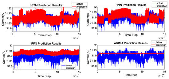
Figure 9.
Comparison of model predictions for Satellite A.
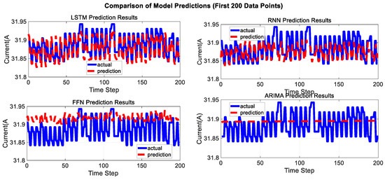
Figure 10.
Comparison of model predictions (first 200 data points) on Satellite A.
The comparison of evaluation metrics for the four algorithms is shown in Table 9.
Table 9.
Comparison of model prediction metrics on Satellite A.
The loss function curves of the three models are shown in Figure 11 below.
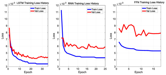
Figure 11.
Training loss history diagram.
It can be seen that the prediction results of the LSTM algorithm are better than those of the other three algorithms.
Satellite “Star B” is selected. A total of 921,897 data points are used, with the first 80% designated as the training set and the remaining 20% as the test set. LSTM, RNN, ARIVAL, and FNN are, respectively, used for prediction. The comparison of prediction results is shown in Figure 12 and Figure 13 below, and the comparison of evaluation indicators of the four algorithms is shown in Table 10 below.
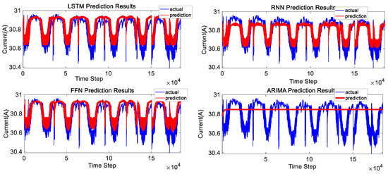
Figure 12.
Comparison of model predictions on Satellite B.
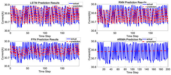
Figure 13.
Comparison of model predictions on Satellite B (first 200 data points).
Table 10.
Comparison of model prediction metrics on Satellite B.
Due to the characteristics of the telemetry transmission mechanism of on-orbit satellites, the distribution of actual satellite telemetry data points is not uniform. When the satellite is within the domestic coverage area, its telemetry data is transmitted at a frequency of 1 s per packet; when the satellite is outside the domestic coverage area, the frequency of telemetry frame data transmitted via inter-satellite links is reduced to 1 min per packet. Additionally, influenced by factors such as mission planning, satellite telemetry data may exhibit periodic invisibility. These transmission characteristics directly result in the non-uniform distribution of the time series of the solar array current output in Figure 10:
Domestic phase: Data sampling is dense, and the current curve shows a smooth semi-sinusoidal shape with a well-defined arc.
Overseas phase: Due to the reduced telemetry update frequency, the sinusoidal spikes in the current curve decay more rapidly.
The prediction model proposed in this study effectively adapts to complex scenarios with uneven telemetry updates by introducing time phase as an input variable. In contrast, the telemetry data of Satellite A lacks significant orbital periodic characteristics, so its prediction model does not require time phase input and only needs load current as the sole characteristic factor—when the load changes, the solar array output current fluctuates correspondingly.
It can be seen that the prediction results of the LSTM algorithm are better than those of the other three algorithms.
6. Conclusions
Combined with the topology of the satellite power system, this paper reveals the influence mechanism of load current as a short-period characteristic factor on the output of the solar array by analyzing the dynamic compensation characteristics of the power regulation module. MEA is highly correlated with the load current. Additionally, it innovatively introduces the faulty wing current input for fault wing scenarios. Meanwhile, LSTM, RNN, and FFN prediction frameworks based on dynamic load characteristics are proposed to reveal their internal correlations with the output fluctuations of the solar array. High-precision adaptive current prediction in dual scenarios of load fluctuations and solar array faults is achieved. The research results provide a data-driven new paradigm for dynamic early warning of spacecraft power systems, which can support on-orbit real-time adjustment of shunt strategies and optimize energy allocation efficiency.
Author Contributions
Conceptualization, H.L.; methodology, H.L. and C.K.; software, H.L.; validation, H.L.; formal analysis, H.L.; investigation, H.L. and C.K.; resources, C.K., Y.S., B.L. and X.W.; data curation, H.L.; writing—original draft preparation, H.L.; writing—review and editing, H.L.; visualization, Q.Z.; supervision, C.K. and Q.Z.; project administration, C.K., Y.S., B.L. and X.W.; funding acquisition, Y.S., B.L. and X.W. All authors have read and agreed to the published version of the manuscript.
Funding
This research received no external funding.
Data Availability Statement
The data presented in this study are available in the article.
Conflicts of Interest
The authors declare no conflict of interest.
Abbreviations
The following abbreviations are used in this manuscript:
| MEA | Main Error Amplifier |
| LEO | Low-Earth Orbit |
| SSA | Spacecraft Solar Arrays |
| MEO | Medium Earth Orbit |
| ANN | Artificial Neural Network |
| RF | Random Forest |
| S3R | Sequential Switching Shunt Regulator |
| SADM | Solar Array Drive Mechanism |
References
- Xi, C.; Liu, Y.; Lin, B.; Wang, X.; Jiang, G.; Kong, C. Radiation Resistance Design of Triple-Junction Gallium Arsenide Solar Arrays for Geosynchronous Satellites. Acta Energiae Solaris Sin. 2022, 43, 9–13. [Google Scholar] [CrossRef]
- Li, Q.; Li, J.; Cao, J.; Li, H. Estimation of power attenuation of solar arrays of LEO satellites. J. Spacecr. TTC Technol. 2017, 36, 207–211. [Google Scholar]
- Chen, B.; Fang, H.; Ma, H.; Luo, K.; Li, R. Modeling and predicting output power losses of solar arrays in a particle filtering framework. In Proceedings of the 2013 IEEE 11th International Conference on Electronic Measurement & Instruments, Harbin, China, 16–19 August 2013; pp. 529–535. [Google Scholar] [CrossRef]
- Gao, Y.; Xu, G.; Wang, S.; Li, Y.; Cai, R.; Li, Z. Solar Array Power Prediction for Near-Space Vehicles Based on a Hybrid Method. IEEE Access 2022, 10, 123233–123250. [Google Scholar] [CrossRef]
- Zhang, Y.; Yan, W.; Su, J.; Hao, J. Power Supply Model and Mission Planning Method for Sun-Synchronous Orbit Satellite Power Systems. J. Northwestern Polytech. Univ. 2019, 37, 1–7. [Google Scholar]
- Peng, M.; Wang, W.; Wu, J.; Li, M. Study on Attenuation Factor of Si Solar Array for Satellite in Sun Synchronous Orbit. Spacecr. Eng. 2011, 20, 61–67. [Google Scholar]
- Jing, Y.; Sun, H.; Lei, Y. Analysis on Performance of Solar Array for Satellite in Sun Synchronous Orbit. Spacecr. Eng. 2013, 22, 61–66. [Google Scholar]
- Xiong, X.; Zhang, M.; Zhao, H.; Jin, D.; Jia, M. Solar-Array Attenuation Analysis Method for Solar Synchronous Orbit Satellites. In Proceedings of the 2023 14th International Conference on Reliability, Maintainability and Safety (ICRMS), Urumuqi, China, 26–29 August 2023; pp. 232–237. [Google Scholar] [CrossRef]
- Yu, H.; Pan, Y.; Li, X.; Guo, W. Degradation assessment of solar cell array of low orbit satellite in orbit. In Proceedings of the 2022 IEEE International Conference on Electrical Engineering, Big Data and Algorithms (EEBDA), Changchun, China, 25–27 February 2022; pp. 21–23. [Google Scholar] [CrossRef]
- Li, Q.; Li, J.; Cao, J.; Li, H. Power Attenuation Estimation of Triple-Junction Gallium Arsenide Solar Arrays for Twilight Orbit Satellites. Space Electron. Technol. 2019, 16, 89–96. [Google Scholar]
- Liao, J.; Jiang, Y.; Liao, H.; Xiao, D.; Yuan, J.; Yang, Z.; Li, J.; Luo, S. Investigation on the effects of shadow on output performance and thermal characteristic of the solar array on stratospheric aerostat. Energy 2019, 182, 765–776. [Google Scholar] [CrossRef]
- Mokhtar, A.; Ibrahim, M.; Hanafy, M.E.; ElTohamy, F.H.A.; Elhalwagy, Y.Z. Developing a modelling environment of spacecraft solar array in low Earth orbit using real-time telemetry data. Frankl. Open 2025, 11, 100268. [Google Scholar] [CrossRef]
- Saravanan, S.; Kumar, R.S.; Balakumar, P.; Prabaharan, N. Optimal power harvesting under partial shading: Binary Greylag Goose optimization for reconfiguration and Machine learning-Based fault diagnosis in solar PV arrays. Energy Convers. Manag. 2025, 333, 119808. [Google Scholar] [CrossRef]
- Sunori, S.K.; Jain, S.; Juneja, P.; Mittal, A. ANN and Random Forest based Prediction of Power Output of Solar Panel. In Proceedings of the 2024 5th International Conference on Smart Electronics and Communication (ICOSEC), Trichy, India, 18–20 September 2024; IEEE: Piscataway, NJ, USA, 2024. [Google Scholar]
- Chen, X.; Wang, S.; Zhang, H. Research on normalized diagnosis method for output current of LEO satellite solar array. In Proceedings of the 9th International Symposium on Test Automation & Instrumentation (ISTAI 2022), Online Conference, Beijing, China, 11–13 November 2022; IET: London, UK, 2022; Volume 2022. [Google Scholar]
- Al-Qawabah, S.; Abu Shaban, N.; Al Aboushi, A.; Al-Salaymeh, A.; Al-Maaitah, A.; Abdelhafez, E. Prediction of the output of the tri-generation concentrated solar power system based on artificial neural network. In Proceedings of the 2024 6th Global Power, Energy and Communication Conference (GPECOM), Budapest, Hungary, 4–7 June 2024; IEEE: Piscataway, NJ, USA, 2024. [Google Scholar]
- Şenol, H.; Çolak, E.; Oda, V. Forecasting of biogas potential using artificial neural networks and time series models for Türkiye to 2035. Energy 2024, 302, 131949. [Google Scholar] [CrossRef]
- Yan, G.; Han, Y.; Wang, Q.; Lin, B.; Su, J. Current Prediction of Solar Array Based on BP Neural Network Optimized by Artificial Bee Colony. J. Nanjing Univ. Aeronaut. Astronaut. 2023, 55, 116–122. [Google Scholar] [CrossRef]
- Zuo, Z.; Jin, D.; Tian, H. Study on Fitting Algorithm for Output Current of Solar Arrays on GEO Satellites. Spacecr. Eng. 2017, 26, 84–90. [Google Scholar]
- Ahn, J.; Lee, Y.; Han, B.; Lee, S.; Kim, Y.; Chung, D.; Jeon, J. A highly effective and robust structure-based LSTM with feature-vector tuning framework for high-accuracy SOC estimation in EV. Energy 2025, 325, 136134. [Google Scholar] [CrossRef]
- Cao, X.; Zhao, W.; Jiang, D.; Zhang, Z.; Liu, M.; Wang, L.; Wang, Z.; Fan, J.; Shi, K. Analysis of thermoelectric coupling under parallel mismatch in triple-junction GaAs solar cells for satellites. Sol. Energy Mater. Sol. Cells 2024, 278, 113197. [Google Scholar] [CrossRef]
- Song, D.; Rehman, M.S.U.; Deng, X.; Xiao, Z.; Noor, J.; Yang, J.; Dong, M. Accurate solar power prediction with advanced hybrid deep learning approach. Eng. Appl. Artif. Intell. 2025, 148, 110367. [Google Scholar] [CrossRef]
- Tempola, F.; Musdholifah, A.; Wardoyo, R. Analysis of Feature Selection Methods On Clove Quality Classification. In Proceedings of the 2024 8th International Conference on Information Technology (InCIT), Chonburi, Thailand, 14–15 November 2024; pp. 337–340. [Google Scholar] [CrossRef]
- Zhi, S.; Shi, J.; Si, X.; Chen, Y.; Ji, Z.; Wan, C. Stability Analysis and Research of SAR Satellite Power Supply System. J. Electr. Eng. Technol. 2024, 19, 2195–2203. [Google Scholar] [CrossRef]
- Rojas, J.J.; Takashi, Y.; Cho, M. A lean satellite electrical power system with direct energy transfer and bus voltage regulation based on a bi-directional buck converter. Aerospace 2020, 7, 94. [Google Scholar] [CrossRef]
- Krummann, W. Next generation GOES satellite power subsystem. IEEE Aerosp. Electron. Syst. Mag. 2002, 16, 23–28. [Google Scholar] [CrossRef]
- Park, J.-E. A Control Algorithm for Tapering Charging of Li-Ion Battery in Geostationary Satellites. Energies 2023, 16, 5636. [Google Scholar] [CrossRef]
- Lei, W.; Li, Y. Simulation Research and Implementation of S4R Power Regulation Technology in Spacecraft. J. Astronaut. 2008, 29, 978–980. [Google Scholar]
- Bao, Z.; Zhu, H.; Wang, M. Low Output Impedance Solar Array Shunt Regulator Based on S3R Architecture. Proc. CSEE 2010, 30, 192–198. [Google Scholar] [CrossRef]
- Cai, X.; Du, Q.; Xia, N.; Wang, C. Design and Verification of the Power Supply and Distribution System for the Chang’e-5 Probe. J. Astronaut. 2021, 42, 1015–1026. [Google Scholar]
- Liang, X.; Ren, X.; Ding, R.; Zhou, Y.; Xian, K. Design and Verification of the Energy System for the Space Station Core Module. Sci. China: Technol. Sci. 2022, 52, 1345–1354. [Google Scholar] [CrossRef]
- Ventosinos, F.; Klusacek, J.; Finsterle, T.; Kunzel, K.; Haug, F.-J.; Holovsky, J. Shunt quenching and concept of independent global shunt in multijunction solar cells. IEEE J. Photovolt. 2018, 8, 1005–1010. [Google Scholar] [CrossRef]
- Mahmoud, Y.; Xiao, W. Evaluation of shunt model for simulating photovoltaic modules. IEEE J. Photovolt. 2018, 8, 1818–1823. [Google Scholar] [CrossRef]
- Blaga, C.; Christmann, G.; Boccard, M.; Ballif, C.; Nicolay, S.; Kamino, B.A. Palliating the efficiency loss due to shunting in perovskite/silicon tandem solar cells through modifying the resistive properties of the recombination junction. Sustain. Energy Fuels 2021, 5, 2036–2045. [Google Scholar] [CrossRef]
- Schirone, L.; Ferrara, M.; Granello, P.; Paris, C.; Pellitteri, F. Power bus management techniques for space missions in low earth orbit. Energies 2021, 14, 7932. [Google Scholar] [CrossRef]
- Orts, C.; Garrigós, A.; Marroquí, D.; Franke, A. Sequential switching shunt regulation using DC transformers for solar array power processing in high voltage satellites. IEEE Trans. Aerosp. Electron. Syst. 2023, 60, 421–429. [Google Scholar] [CrossRef]
- Jiang, Z.; Liu, S.; Dougal, R.A. Design and testing of spacecraft power systems using VTB. IEEE Trans. Aerosp. Electron. Syst. 2003, 39, 976–989. [Google Scholar] [CrossRef]
- Jin, X.; Lin, H.; Yao, W.; Lu, Z. Sequential switching shunt regulator with improved controller to suppress the influence of double-section phenomenon. IEEE J. Emerg. Sel. Top. Power Electron. 2022, 10, 5318–5331. [Google Scholar] [CrossRef]
- Prakash, S.; Jalal, A.S.; Pathak, P. Forecasting COVID-19 pandemic using prophet, lstm, hybrid gru-lstm, cnn-lstm, bi-lstm and stacked-lstm for India. In Proceedings of the 2023 6th International Conference on information systems and computer networks (ISCON), Mathura, India, 3–4 March 2023; IEEE: Piscataway, NJ, USA, 2023. [Google Scholar]
- Diaaeldin, A.; Zaher, M. Enhancing Road Safety: Leveraging CNN-LSTM and Bi-LSTM Models for Advanced Driver Behavior Detection. In Proceedings of the 2024 Intelligent Methods, Systems, and Applications (IMSA), Giza, Egypt, 13–14 July 2024; IEEE: Piscataway, NJ, USA, 2024. [Google Scholar]
- Chakraborty, S.; Banik, J.; Addhya, S.; Chatterjee, D. Study of Dependency on number of LSTM units for Character based Text Generation models. In Proceedings of the 2020 International Conference on Computer Science, Engineering and Applications (ICCSEA), Gunupur, India, 13–14 March 2020; IEEE: Piscataway, NJ, USA, 2023. [Google Scholar]
- Gill, K.S.; Anand, V.; Chauhan, R.; Choudhary, A.; Gupta, R. CNN, LSTM, and Bi-LSTM based Self-Attention Model Classification for User Review Sentiment Analysis. In Proceedings of the 2023 3rd International Conference on Smart Generation Computing, Communication and Networking (SMART GENCON), Bangalore, India, 29–31 December 2023; IEEE: Piscataway, NJ, USA, 2024. [Google Scholar]
- Huang, S.; Zeng, Z.; Jiang, S. Generalization bounds for pairwise learning with the Huber loss. Neurocomputing 2025, 622, 129265. [Google Scholar] [CrossRef]
- Nguinabé, J.; Rockefeller, R.; Khan, N.M.; Rodrigues, P.C. Bootstrap prediction intervals for the long short term memory (LSTM) recurrent neural network. Expert. Syst. Appl. 2025, 284, 127728. [Google Scholar] [CrossRef]
- Siddique, M.A.B.; Mahalder, B.; Haque, M.M.; Ahammad, A.K.S. Forecasting air temperature and rainfall in Mymensingh, Bangladesh with ARIMA: Implications for aquaculture management. Egypt. J. Aquat. Res. 2025, in press. [Google Scholar] [CrossRef]
- Kong, C.; Liu, H.; Lin, B.; Wang, X.; Zhang, Q.; Wang, Y. Energy Adaptability Analysis Based on the Stall Fault of Solar Array Drive Assembly for Medium Earth Orbit Satellite. Energies 2025, 18, 2315. [Google Scholar] [CrossRef]
Disclaimer/Publisher’s Note: The statements, opinions and data contained in all publications are solely those of the individual author(s) and contributor(s) and not of MDPI and/or the editor(s). MDPI and/or the editor(s) disclaim responsibility for any injury to people or property resulting from any ideas, methods, instructions or products referred to in the content. |
© 2025 by the authors. Licensee MDPI, Basel, Switzerland. This article is an open access article distributed under the terms and conditions of the Creative Commons Attribution (CC BY) license (https://creativecommons.org/licenses/by/4.0/).