A Neural Network-Based Fault-Tolerant Control Method for Current Sensor Failures in Permanent Magnet Synchronous Motors for Electric Aircraft

Abstract

To enhance the reliability of electric propulsion in electric aircraft and address power interruptions caused by current sensor failures, this study proposes a current sensorless fault-tolerant control strategy for permanent magnet synchronous motors (PMSMs) based on a long short-term memory (LSTM) network. First, a hierarchical architecture is constructed to fuse multi-phase electrical signals in the fault diagnosis layer (sliding mode observer). A symbolic function for the reaching law observer is designed based on Lyapunov theory, in order to generate current predictions for fault diagnosis. Second, when a fault occurs, the system switches to the LSTM reconstruction layer. Finally, gating units are used to model nonlinear dynamics to achieve direct mapping of speed/position to phase current. Verification using a physical prototype shows that the proposed method can complete mode switching within 10 ms after a sensor failure, which is 80% faster than EKF, and its speed error is less than 2.5%, fully meeting the high speed error requirements of electric aircraft propulsion systems (i.e., ≤3%). The current reconstruction RMSE is reduced by more than 50% compared with that of the EKF, which ensures continuous and reliable control while maintaining the stable operation of the motor and realizing rapid switching. The intelligent algorithm and sliding mode control fusion strategy meet the requirements of high real-time performance and provide a highly reliable fault-tolerant scheme for electric aircraft propulsion.

1. Introduction

The global aviation industry’s shift toward green technologies has positioned electric aircraft as a key research focus for short-haul transport and emergency services, driven by their zero-emission operation, low noise, and energy efficiency [1,2,3]. Permanent magnet synchronous motors (PMSMs) have become the preferred propulsion solution for electric aircraft due to their high power density, rapid dynamic response, and operational reliability [4,5]. In PMSM field-oriented control systems, current sensors provide critical real-time data for precision control. However, harsh operational conditions (extreme temperatures, vibration, electromagnetic interference) can cause sensor failures, potentially destabilizing motor control systems and compromising flight safety through power interruptions [6]. Consequently, the development of fault-tolerant control methods which can handle current sensor failures has emerged as a critical priority in advancing electric aircraft technology.

Conventional control architectures rely heavily on current sensors for torque–flux decoupling through stator current measurements [7]. Aviation environments exacerbate sensor failure risks [8], with international safety reports indicating that 15% of electric aircraft malfunctions originate from sensor faults [9]. Existing sensorless control methods face limitations in terms of parameter sensitivity and dynamic robustness [10,11]. Sliding mode observer (SMO) techniques demonstrate susceptibility to resistance/inductance variations, with accuracy degradation exceeding 8% after 500 operational hours due to component aging [12]. Similarly, while extended Kalman filter (EKF) techniques effectively reduce noise interference [13], their high computational complexity makes their real-time implementation in embedded controllers challenging. Furthermore, these methods frequently exhibit phase delays during high-speed operations or under abrupt load changes, compromising control stability [14]. This underscores the critical need for current reconstruction approaches that simultaneously achieve high precision, low computational demands, and adaptability to parameter variations to ensure reliable electric aircraft propulsion systems.

Recent advances in sensorless control have been focused on observer optimization and multi-source data fusion. While adaptive SMO designs reduce chattering through dynamic gain adjustment [15,16,17], they require complex parameter tuning and neglect nonlinear motor characteristics. Refs. [18,19] integrated a Luenberger observer with model predictive control (MPC) to enhance dynamic response speed; however, the approach incurred significant computational overhead, rendering it impractical for real-time implementation. Meanwhile, data-driven methods have emerged as promising alternatives for sensorless control [20]. For instance, a support vector machine (SVM) was employed for motor current regression prediction, although its generalization capability was constrained by the limited scope of the used training data [21,22]. Similarly, a deep belief network (DBN) was applied in [23,24] to effectively extract motor operation features; however, it exhibited gradient vanishing issues in time-series modeling, thereby limiting its ability to capture long-term dependencies. Notably, long short-term memory (LSTM) networks—a specialized type of recurrent neural network (RNN)—demonstrate exceptional capabilities in time-series prediction due to their gated memory architecture [25,26]. While initial applications focused on motor speed and load torque estimation demonstrated the effectiveness of LSTMs in modeling nonlinear systems [27], subsequent integration with extended Kalman filters (EKF) improved their positioning accuracy in UAV navigation scenarios under turbulent conditions [28,29]. However, existing implementations focus primarily on ground vehicles and drones, lacking optimization for the high-dynamic, high-disturbance operational conditions specific to aviation systems. Furthermore, conventional LSTM implementations require computationally intensive online training and have excessive memory footprints, making them impractical for deployment on resource-constrained embedded platforms [30]. Solidifying network weights through offline training while maintaining adaptability to changes in motor parameters remains an underexplored area in the existing literature.

In summary, we propose a hybrid fault-tolerant control method integrating sliding mode observation with LSTM-based temporal modeling. This co-design approach synergizes the complementary strengths of both techniques to overcome their individual limitations. The specific innovations are reflected in the following aspects: A sliding mode dynamic observer is designed to capture the transient high-frequency disturbance characteristics of the current (such as the mutation signal caused by sensor failure) in real-time, which are used as an additional input to the LSTM network to make up for the limitations of traditional LSTMs in terms of timing modeling in noise-sensitive scenarios [31,32]. Adaptive switching gains ($K_s$) extract signal differential characteristics ($\Delta id$, $\Delta iq$), which are combined with conventional LSTM inputs (rotational speed/position) to create multi-modal input vectors. This integration improves the fault detection sensitivity compared to standalone architectures.

The developed LSTM-based control strategy for PMSM systems achieves real-time current reconstruction through offline-trained models, maintaining continuous operation during sensor faults. The innovation is further expanded to the following four aspects: Gating mechanism and dynamic feature extraction: Through the synergy of forgetting gates, input gates, and output gates, the LSTM network can adaptively select the weights for historical information and current inputs, effectively capturing the long-term dependence and nonlinear dynamic characteristics of motor current signals. Embedded Optimization: Offline-trained models reduce real-time computation to matrix operations, achieving lower overhead than conventional observer methods while meeting real-time requirements. Enhanced parameter robustness: By training the network on motor parameter perturbation data, the model can still maintain high-precision prediction when parameters such as resistance and inductance change, overcoming the inherent defects of traditional observers. Sliding mode–LSTM collaborative anti-noise mechanism: The forget gate design of the LSTM integrates the robustness index of the sliding mode observer, dynamically adjusts the weight attenuation coefficient of historical noise data, and suppresses the accumulated error after sensor failure.

This study implements a dual-layer fault-tolerant architecture integrating sliding mode fault diagnosis with LSTM-based current reconstruction. The experimental results show that the proposed method can complete mode switching within 10 ms after a current sensor fails, the speed error is less than 2.5%, and the calculation delay is reduced by 80% when compared with the traditional EKF. The following chapters systematically explain the proposed method’s design, experimental verification, and prospects for engineering application.

2. System Design and Control Architecture

2.1. Electric Propulsion System Configuration

To prevent propulsion system failures caused by current sensor malfunctions in electric aircraft, this study introduces an LSTM-based current reconstruction method that enhances operational reliability while maintaining flight safety. The developed control system architecture (Figure 1) integrates voltage/current sensing modules, fault diagnosis units, Clark transformation, space vector PWM (SVPWM), and inverter components with the LSTM network. The operational workflow initiates with three-phase voltage and two-phase current measurements from motor cables. A Clark transformation is performed to convert these to α-β frame voltages (uα, uβ) for fault diagnosis. A sliding mode observer then generates predicted currents (${\widehat{i}}_{\alpha }$, ${\widehat{i}}_{\beta }$), which are compared against the Clark-transformed measured currents ($i_{\alpha }$, $i_{\beta }$). A 5% error threshold triggers the fault response: <5% maintains normal operation (Switch 1), while an error exceeding 5% activates LSTM-based reconstruction (Switch 2). Position sensor signals are converted into speed parameters, which serve as inputs to the LSTM network to predict dq-axis currents ($i_d$, $i_q$). These predictions are subsequently fed into PI controllers to generate voltage references ($u_d$, $u_q$), followed by inverse Park transformation to derive α-β frame voltages ($u_{\alpha }$, $u_{\beta }$). Finally, space vector PWM (SVPWM) is performed to convert these voltages into gate signals for the inverter, ultimately producing three-phase AC power to drive the motor.

2.2. Electric Propulsion System Design

Voltage Sensing Module

Voltage sensors installed on the three-phase motor cables measure the phase voltages ($u_a$, $u_b$, $u_c$). These measurements undergo Clark transformation, converting the three-phase voltages into two-phase AC voltages ($u_{\alpha }$, $u_{\beta }$) in the stationary coordinate system.

$$\left[\begin{array}{c}{u}_{\alpha }\\ u_{\beta }\end{array}\right]=\left[\begin{array}{lll}{\displaystyle \frac{2}{3}}\hfill & -{\displaystyle \frac{1}{3}}\hfill & -{\displaystyle \frac{1}{3}}\hfill \\ 0\hfill & {\displaystyle \frac{\sqrt{3}}{3}}\hfill & -{\displaystyle \frac{\sqrt{3}}{3}}\hfill \end{array}\right]\left[\begin{array}{c}{u}_a\\ u_b\\ u_c\end{array}\right]$$

(1)

Current Sensing Module

Similarly, current sensors on the three-phase cables measure two-phase currents ($i_a$, $i_b$), which are transformed via Clark current conversion into two-phase currents ($i_{\alpha }$, $i_{\beta }$) in the stationary coordinate system.

$$\left[\begin{array}{c}{i}_{\alpha }\\ i_{\beta }\end{array}\right]=\left[\begin{array}{cc}1& 0\\ {\displaystyle \frac{1}{\sqrt{3}}}& {\displaystyle \frac{2}{\sqrt{3}}}\end{array}\right]\left[\begin{array}{c}{i}_a\\ i_b\end{array}\right]$$

(2)

Position Acquisition Module

The position acquisition module measures the rotor’s angular position $\theta$ in the permanent magnet synchronous motor (PMSM) via an integrated position sensor.

$$\omega ={\displaystyle \frac{d\theta }{dt}}$$

(3)

The mechanical angular velocity ($\omega$) is derived from the motor’s position angle ($\theta$) through differentiation.

The rotational speed ($n$) can then be expressed as:

$$n=\omega {\displaystyle \frac{30}{\pi }}$$

(4)

where $n$ is the motor speed.

Velocity PI

The speed PI controller operates as the outer loop to regulate motor velocity.

The speed error is calculated as follows:

$$e_n=n_{ref}-n$$

(5)

where $n_{ref}$ denotes the reference speed, $n$ represents the measured speed, and $e_n$ is the difference between these speeds.

The PI controller generates the torque reference as follows:

$$T_{ref}=K_{p,n}{e}_n+K_{i,n}{\displaystyle \int e_{n}dt}$$

(6)

where $T_{ref}$ is the reference torque, and $K_{p,n}$ and $K_{i,n}$ are the proportional and integral gains, respectively.

Torque-to-current conversion is implemented through:

$$I_{qref}={\displaystyle \frac{T_{ref}}{K_t}}$$

(7)

where $I_{qref}$ is the desired q-axis current and $K_t$ is the torque constant of the motor.

Current PI

The current PI is the inner loop, and its control goal is to regulate the stator current such that it reaches the target value on the dq axis.

The current error is calculated as:

$$e_d=i_{dref}-i_d,e_q=i_{qref}-i_q$$

(8)

where $i_{dref}$ is the expected current in the d-axis, $i_d$ and $i_q$ are the actual currents in the d- and q-axes, and $e_d$ and $e_q$ are the differences between the expected and actual currents in the d- and q-axes, respectively.

The voltage control quantity is calculated using the PI controller, as follows:

$$\left\{\begin{array}{c}{u}_d=K_{p,d}{e}_d+K_{i,d}{\displaystyle \int e_{d}dt}\\ u_q=K_{p,q}{e}_q+K_{i,q}{\displaystyle \int e_{q}dt}\end{array}\right.$$

(9)

where $u_d$ and $u_q$ are the voltages in the d- and q-axes, which are used to generate the SVPWM signal; $K_{p,d}$ and $K_{p,q}$ are the proportional gains of the current error in the d- and q-axes; and $K_{i,d}$ and $K_{i,q}$ are the integral gains of the current errors in the d- and q-axes, respectively.

After calculating $u_d$ and $u_q$, the inverse Park transform is calculated as follows:

$$\left[\begin{array}{c}{u}_{\alpha }\\ u_{\beta }\end{array}\right]=\left[\begin{array}{cc}\cos \phi & -\sin \phi \\ \sin \phi & \cos \phi \end{array}\right]\left[\begin{array}{c}{u}_d\\ u_q\end{array}\right]$$

(10)

The transformed dq-axis components ($u_{\alpha }$, $u_{\beta }$) are processed through space vector PWM (SVPWM) to generate duty cycle signals for inverter switching. These signals drive the inverter to produce three-phase AC voltages, ultimately regulating the motor’s operation. The coordinate rotation angle ($\phi$) defines the spatial relationship between the stationary and rotating reference frames.

3. Fault Diagnosis Module Based on Synovial Variable Structure

The fault diagnosis module employs a sliding mode observer in the stationary α-β coordinate frame of the permanent magnet synchronous motor (PMSM). This observer generates predicted currents (${\widehat{i}}_{\alpha }$, ${\widehat{i}}_{\beta }$) using variable structure control, which are compared against the Clark-transformed measured currents ($i_{\alpha }$, $i_{\beta }$) to determine whether the current failure fault has occurred. Sliding mode control (SMC) enables robust regulation for nonlinear systems with uncertainties. The methodology allows for the construction of a sliding surface that drives system states to converge within finite time and maintains sliding motion through Lyapunov-stable dynamics. Its implementation proceeds as follows:

First, in order to obtain the predicted currents a and b, the voltage equation of the permanent magnet synchronous motor in a two-phase stationary coordinate system can be expressed as:

$$\left\{\begin{array}{c}{u}_{\alpha }=R_s{\widehat{i}}_{\alpha }+L_s{\displaystyle \frac{d{\widehat{i}}_{\alpha }}{dt}}-{\psi }_f{\omega }_e\sin \theta \\ u_{\beta }=R_s{\widehat{i}}_{\beta }+L_s{\displaystyle \frac{d{\widehat{i}}_{\beta }}{dt}}+{\psi }_f{\omega }_e\sin \theta \end{array}\right.$$

(11)

where $R_s$ is the stator resistance; ${\widehat{i}}_{\alpha }$ and ${\widehat{i}}_{\beta }$ are the components of the current value estimated by the sliding mode observer in the α- and β-axes; $L_s$ is the inductance of the permanent magnet synchronous motor, where the surface mount type of motor is usually adopted, and the relationship between the d-axis inductance and the q-axis inductance can be expressed as $L_d$ = $L_q$ = $L_s$; ${\psi }_f$ is the flux of a permanent magnet; ${\omega }_e$ is the angular velocity of the motor, where ${\omega }_e={\displaystyle \frac{p}{2}}\cdot \omega$; and $p$ is the number of pole pairs.

The back EMF of a motor in a two-phase stationary coordinate system can be expressed as:

$$\left\{\begin{array}{c}{e}_{\alpha }=-{\psi }_f{\omega }_e\sin \theta \\ e_{\beta }={\psi }_f{\omega }_e\cos \theta \end{array}\right.$$

(12)

where $e_{\alpha }$ and $e_{\beta }$ are the back electromotive forces of the motor in the α- and β-axes of the two-phase stationary coordinate system, respectively.

From Equations (11) and (12), we get:

$$\left\{\begin{array}{c}{u}_{\alpha }=R_s{\widehat{i}}_{\alpha }+L_s{\displaystyle \frac{d{\widehat{i}}_{\alpha }}{dt}}+e_{\alpha }\\ u_{\beta }=R_s{\widehat{i}}_{\beta }+L_s{\displaystyle \frac{d{\widehat{i}}_{\beta }}{dt}}+e_{\beta }\end{array}\right.$$

(13)

From Equation (13), it follows that:

$$\left\{\begin{array}{c}{\displaystyle \frac{d{\widehat{i}}_{\alpha }}{dt}}={\displaystyle \frac{1}{L_s}}(u_{\alpha }-R_s{\widehat{i}}_{\alpha }-e_{\alpha })\\ {\displaystyle \frac{d{\widehat{i}}_{\beta }}{dt}}={\displaystyle \frac{1}{L_s}}(u_{\beta }-R_s{\widehat{i}}_{\beta }-e_{\beta })\end{array}\right.$$

(14)

The motor back EMF can be expressed as a function of the sliding mode control rate:

$$\left\{\begin{array}{c}{e}_{\alpha }={\nu }_{\alpha }=K\cdot sign(s_{\alpha })\\ e_{\beta }={\nu }_{\beta }=K\cdot sign(s_{\beta })\end{array}\right.$$

(15)

where ${\nu }_{\alpha }$ and ${\nu }_{\beta }$ are the sliding mode control rates of the sliding mode observer; $K$ is the sliding mode gain value; sign is a symbolic function; and $s_{\alpha }$ and $s_{\beta }$ are synovial surface functions.

From Equations (14) and (15), we obtain:

$$\left\{\begin{array}{c}{\displaystyle \frac{d{\widehat{i}}_{\alpha }}{dt}}={\displaystyle \frac{1}{L_s}}(u_{\alpha }-R_s{\widehat{i}}_{\alpha }-{\nu }_{\alpha })\\ {\displaystyle \frac{d{\widehat{i}}_{\beta }}{dt}}={\displaystyle \frac{1}{L_s}}(u_{\beta }-R_s{\widehat{i}}_{\beta }-{\nu }_{\beta })\end{array}\right.$$

(16)

The synovial surface function can be expressed as:

$$\left\{\begin{array}{c}{s}_{\alpha }={\tilde{i}}_{\alpha }={\widehat{i}}_{\alpha }-i_{\alpha }\\ s_{\beta }={\tilde{i}}_{\beta }={\widehat{i}}_{\beta }-i_{\beta }\end{array}\right.$$

(17)

To ensure accurate estimation of the current (${\widehat{i}}_{\alpha }$, ${\widehat{i}}_{\beta }$) by the sliding mode observer, the convergence of observation errors ($s_{\alpha }$, $s_{\beta }$) must be rigorously verified. Stability is demonstrated via Lyapunov’s direct method: a candidate Lyapunov function V(s) is defined, where its time derivative must satisfy V(s) < 0 to guarantee finite-time convergence.

First, the Lyapunov function can be expressed as:

$$\left\{\begin{array}{c}V(s_{\alpha })={\displaystyle \frac{1}{2}}{s}_{\alpha }^2\\ V(s_{\beta })={\displaystyle \frac{1}{2}}{s}_{\beta }^2\end{array}\right.$$

(18)

Its derivative is then given as:

$$\left\{\begin{array}{c}{\displaystyle \frac{dV(s_{\alpha })}{dt}}=s_{\alpha }{\displaystyle \frac{d{s}_{\alpha }}{dt}}\\ {\displaystyle \frac{dV(s_{\beta })}{dt}}=s_{\beta }{\displaystyle \frac{d{s}_{\beta }}{dt}}\end{array}\right.$$

(19)

where ${\displaystyle \frac{d{s}_{\alpha }}{dt}}$ and ${\displaystyle \frac{d{s}_{\beta }}{dt}}$ can be expressed as:

$$\left\{\begin{array}{l}\begin{array}{c}{\displaystyle \frac{d{s}_{\alpha }}{dt}}={\displaystyle \frac{1}{L_s}}(u_{\alpha }-R_s{i}_{\alpha }-e_{\alpha })-{\displaystyle \frac{1}{L_s}}(u_{\alpha }-R_s{\widehat{i}}_{\alpha }-K\cdot sign(s_{\alpha }))\\ ={\displaystyle \frac{1}{L_s}}(-R_s{s}_{\alpha }+e_{\alpha }-K\cdot sign(s_{\alpha }))\end{array}\hfill \\ \begin{array}{c}{\displaystyle \frac{d{s}_{\beta }}{dt}}={\displaystyle \frac{1}{L_s}}(u_{\beta }-R_s{i}_{\beta }-e_{\beta })-{\displaystyle \frac{1}{L_s}}(u_{\beta }-R_s{\widehat{i}}_{\beta }-K\cdot sign(s_{\beta }))\\ ={\displaystyle \frac{1}{L_s}}(-R_s{s}_{\beta }+e_{\beta }-K\cdot sign(s_{\beta }))\end{array}\hfill \end{array}\right.$$

(20)

Substituting this into Equation (19) obtains:

$$\left\{\begin{array}{c}{\displaystyle \frac{dV(s_{\beta })}{dt}}={\displaystyle \frac{1}{L_s}}(-R_s{s}_{\alpha }^2+s_{\alpha }{e}_{\alpha }-K\left|s_{\alpha }\right|)\\ {\displaystyle \frac{dV(s_{\beta })}{dt}}={\displaystyle \frac{1}{L_s}}(-R_s{s}_{\beta }^2+s_{\beta }{e}_{\beta }-K\left|s_{\beta }\right|)\end{array}\right.$$

(21)

For error convergence, it is necessary to ensure that:

$$\left\{\begin{array}{c}{\displaystyle \frac{dV(s_{\alpha })}{dt}}<0\\ {\displaystyle \frac{dV(s_{\beta })}{dt}}<0\end{array}\right.$$

(22)

Specifically,

$$\left\{\begin{array}{c}-R_s{s}_{\alpha }^2+s_{\alpha }{e}_{\alpha }-K\left|s_{\alpha }\right|<0\\ -R_s{s}_{\beta }^2+s_{\beta }{e}_{\beta }-K\left|s_{\beta }\right|<0\end{array}\right.$$

(23)

Then, we have:

$$\left\{\begin{array}{c}{s}_{\alpha }{e}_{\alpha }-K\left|s_{\alpha }\right|<0\\ s_{\beta }{e}_{\beta }-K\left|s_{\beta }\right|<0\end{array}\right.$$

(24)

If the equation holds, it can be ensured that the errors $s_{\alpha }$ and $s_{\beta }$ converge to 0, meaning that the observer correctly estimates ${\widehat{i}}_{\alpha }$ and ${\widehat{i}}_{\beta }$.

Take the maximum value:

$$K>\max \left\{\left|e_{\alpha }\right|,\left|e_{\beta }\right|\right\}$$

(25)

From Equation (12), since the amplitude of the sine and cosine functions is at most 1, we have:

$$\left\{\begin{array}{c}\left|e_{\alpha }\right|\le {\omega }_e{\psi }_f\\ \left|e_{\beta }\right|\le {\omega }_e{\psi }_f\end{array}\right.$$

(26)

The maximum value of the back EMF can be expressed as:

$$e_{\max }={\omega }_e{\psi }_f{W}_{fx}$$

(27)

From Equation (20), it can be seen that $K$ should satisfy $K$ > $e_{\max }$. The following condition is desirable:

$$K=1.2\cdot e_{\max }$$

(28)

Bringing K into Equations (14) and (15) gives ${\widehat{i}}_{\alpha }$, ${\widehat{i}}_{\beta }$.

In order to determine the rationality of the fault detection threshold (i.e., balancing between the false alarm rate and detection delay), a PMSM system simulation was carried out (Figure 2), in which three types of typical faults (current sudden change of 0, ±5% deviation, ±10% deviation) were injected to test the performance under different thresholds. The results are as follows:

Based on the above figure, a 5% threshold is optimal to meet the requirements for the false alarm rate and delay at the same time. The specific reasons are as follows: a low false alarm rate (10%) helps to avoid malfunctions under normal working conditions, in line with the stability requirements of aviation systems; the detection delay meets the standard requirements (within 0.05 s) for electric aircraft propulsion systems, thus ensuring a rapid response to faults; in engineering practice, too high a threshold (>5%) will sacrifice real-time performance while a low value (<5%) will cause excessive false alarms. Therefore, a threshold of 5% was considered to achieve the best trade-off.

The selected threshold is 5% and, when ${\widehat{i}}_{\alpha }$ and ${\widehat{i}}_{\beta }$ satisfy Equation (29), it can be determined whether a current sensor failure fault has occurred, in which case $K_s$ is set to 1:

$$\left\{\begin{array}{c}\left|{\widehat{i}}_{\alpha }-i_{\alpha }\right|\ge 5\%i_{\alpha }\\ \left|{\widehat{i}}_{\beta }-i_{\beta }\right|\ge 5\%i_{\beta }\end{array}\right.$$

(29)

If the current sensor is not faulty, $K_s$ is set to 0 and the sum can be obtained by the Park transformation:

$$\left[\begin{array}{c}{i}_d\\ i_q\end{array}\right]=\left[\begin{array}{cc}\cos \theta & \sin \theta \\ -\sin \theta & \cos \theta \end{array}\right]\left[\begin{array}{c}{i}_{\alpha }\\ i_{\beta }\end{array}\right]$$

(30)

where $i_d$ and $i_q$ are the two-phase currents of the motor in the d- and q-axes, respectively.

4. LSTM Current Reconstruction Module

4.1. LSTM Structure

Long short-term memory (LSTM) networks enhance traditional recurrent neural networks (RNNs) by improving their temporal signal processing capabilities. Unlike conventional RNNs, the gated architecture of LSTMs allows for the identification and dynamic regulation of the influence of less relevant sequential inputs through selective memory mechanisms. This enables optimized weighting of contextual information during data processing, making LSTMs particularly effective for time-series analysis. The LSTM architecture comprises three gated structures (input gate, output gate, and forget gate) coupled with a memory cell state (see Figure 3). Each unit implements information filtration and transmission operations through a four-stage processing sequence:

Forget Gate Mechanism: The first operational stage evaluates the relevance of historical information through adaptive gating. This mechanism processes the current input vector $x$ and prior hidden state $h_{j-1}$ through weight matrices ($W_{fx}$, $W_{fh}$) and a bias vector $b_f$, and a gating value between 0 and 1 is generated via the Sigmoid activation function. This gating value dynamically regulates the flow of information by attenuating insignificant historical features while preserving critical temporal dependencies. The value $f_j$ of the forget gate is calculated as follows:

$$f_j=\sigma (W_{fx}{x}_j+W_{fh}{h}_{j-1}+b_f)$$

(31)

Information Update Phase: The LSTM regulates cell state updates through an input gating mechanism, selectively integrating new temporal information while preserving long-term dependencies. This phase employs dual computational pathways: (1) The input gate $i_j$ filters current inputs via sigmoid activation, and (2) the candidate state vector ${\tilde{c}}_j$ encodes potential state updates. These parallel computations combine sigmoid-gated filtering (range: 0–1) and tanh-modulated feature scaling (range: −1 to 1) in order to optimize temporal information fusion. The implementation comprises two core operations:

$$\begin{array}{l}{i}_j=\sigma (W_{ix}{x}_j+W_{ih}{h}_{j-1}+b_i)\\ {\tilde{c}}_j=\tanh (W_{cx}{x}_j+W_{ch}{h}_{j-1}+b_j)\end{array}$$

(32)

Once the values of $f_j$, $i_j$, and ${\tilde{c}}_j$ have been determined, the new element state $c_j$ can be calculated from the product of the vector elements (denoted as ⊙):

$$c_j=f_j\odot c_{j-1}+i_j\odot {\tilde{c}}_j$$

(33)

The information processing process realizes hierarchical regulation through the gating mechanism: the first-stage gating filtering operation (corresponding to the first multiplication step in Equation (32)) is responsible for dynamically adjusting the intensity of historical memory, and the active attenuation of non-relevant information is realized through the weight coefficient of the forget gate. The second-stage gating operation (corresponding to the second multiplication step in Equation (32)) establishes a collaborative update mechanism between the input gate and the candidate state vectors, completing the selective integration of the temporal feature vectors.

The generation of the final output vector follows the principle of gated state modulation: the output gate $o_j$ performs multi-dimensional parameter fusion based on the current cell state $c_j$, input feature $x_j$, and the previous output $h_{j-1}$, and generates the output gating coefficient through the Sigmoid function. The coefficient is multiplied by the unit state normalized by the tanh function to generate the output $h_j$ containing the temporal correlation features, thus realizing the controllable transmission of memory information in the time dimension:

$$\begin{array}{l}{o}_j=\sigma (W_{ox}{x}_j+W_{oh}{h}_{j-1}+b_o)\\ h_j=o_j\odot \tanh (c_j)\end{array}$$

(34)

4.2. Training of LSTM Networks

The differentiable gated architecture of LSTM units provides a theoretical foundation for network training. Each gate employs continuously differentiable activation functions, enabling seamless integration into gradient-based optimization frameworks through end-to-end backpropagation. Training requires the definition of an objective function $E({\eta }_j)$, allowing for gradient descent to iteratively optimize parameters via backpropagation. This minimizes prediction errors through incremental weight adjustments across the network. During implementation, weight matrices are updated after each forward pass using chain rule-derived gradients. Based on the update rules used in the derivation of the formula, the network parameters are iteratively updated in the negative direction of the loss function gradient, which ensures the effective convergence of the model on the error surface through use of the following formula:

$${\eta }_{j+1}={\eta }_j-\alpha \nabla E({\eta }_j)$$

(35)

where $\eta$ is the parameter vector, $j$ is the number of iterations, $\alpha$ > 0 is the learning rate, and $E({\eta }_j)$ is the objective function.

The recurrent nature of LSTM networks presents dual challenges for gradient-based optimization: (1) Deep temporal dependencies induce abnormal gradient dynamics, manifesting as gradient explosion or vanishing phenomena. These instabilities distort parameter update trajectories from optimal convergence paths, significantly degrading training efficacy. (2) Fixed learning rates cause imbalanced update magnitudes due to gradient norm fluctuations. Particularly, diminished gradient magnitudes lead to undersized parameter updates, resulting in abrupt convergence slowdowns. To address these challenges, we implement the Adam (adaptive moment estimation) optimizer. This algorithm enables time-varying step size adaptation through dynamic maintenance of gradient first-moment (mean) and second-moment (variance) estimates. As shown in Equation (36), Adam not only realizes adaptive adjustment of the learning rate but also effectively suppresses gradient oscillations through the momentum accumulation mechanism, which significantly improves the training efficiency and stability of LSTM networks when compared with the traditional gradient descent method.

$$\begin{array}{l}{m}_j={\beta }_1{m}_{j-1}+(1-{\beta }_1)\nabla E({\eta }_j)\\ v_j={\beta }_2{v}_{j-1}+(1-{\beta }_2){\left[\nabla E({\eta }_j)\right]}^2\\ {\widehat{m}}_j={\displaystyle \frac{m_j}{\sqrt{1-{\beta }_1^j}}}\\ {\widehat{v}}_j={\displaystyle \frac{v_j}{\sqrt{1-{\beta }_2^j}}}\\ {\theta }_j={\theta }_{j-1}-{\displaystyle \frac{a{\widehat{m}}_j}{\sqrt{{\widehat{v}}_j+}\epsilon }}\end{array}$$

(36)

The algorithm updates the exponential moving average $m_j$ of the gradient and the exponential moving average $v_j$ of the squared gradient at each step. The parameters ${\beta }_1$, ${\beta }_2$ ∈ [0, 1] control the rate at which the historical values influence the current moving average decays. The vectors $m_0$ and $v_0$ are initialized to zero. Therefore, the moving average is shifted towards zero, and the corrected values of ${\widehat{m}}_j$ and ${\widehat{v}}_j$ are calculated. ${\beta }_1^j$ and ${\beta }_2^j$ represent exponential operations, where the exponents are $j$. The factor $\epsilon$ takes a very small value in the equation to avoid division by zero. In many cases, $\alpha$ = 0.001, ${\beta }_1$ = 0.9, ${\beta }_2$ = 0.999, and $\epsilon ={10}^{-8}$ are considered good values to start trying to train the network. The adaptive learning rate strategy was adopted: the initial learning rate was assessed using a grid search (range: 0.1 to 1 × 10⁻⁵), and 0.001 was determined to perform best in the validation set, in terms of the loss decline rate and stability. The Adam parameters (${\beta }_1$ = 0.9, ${\beta }_2$ = 0.999) were set following the machine learning literature [33], allowing its momentum mechanism to mitigate gradient oscillations, which is suitable for motor non-stationary timing data. All networks described in the following sections were also trained with these parameters.

4.3. LSTM Network Training for Stator Current Prediction Based on Motor Speed and Position Without Current Sensors

The proposed network architecture comprises two independent LSTM models (a velocity model and a position model) with identical configurations. Considering the strict real-time requirements of aviation motor control systems (response time needs to be <30 ms), the inference delay will be significantly increased when using overly deep networks (≥3 layers), while single-layer networks have difficulty in capturing the nonlinear timing dependence under high-speed dynamics. Therefore, a two-layer structure was considered to achieve the optimal balance between delay and accuracy. The number of neurons was set as 64 → 32: the first layer of 64 neurons is responsible for high-frequency feature extraction (such as current transient mutations), while the second layer of 32 neurons compresses the feature dimension to reduce the amount of computation [34]. A batch size of 32 maximizes data diversity under GPU memory constraints, improves training speed compared to a batch size of 16, and ensures stabler convergence than when using a batch size of 64 [35]. Comparative experiments showed that the overfitting is significant without Dropout (with a training/validation MAE gap as high as 35%), and the network training effect was found to be optimal when Dropout = 0.2 after multiple different Dropout experiments.

Each model receives a two-dimensional input tensor (speed and position) containing 50 timesteps through the input layer. The hidden layer consists of: (i) a two-dimensional LSTM layer with 64 units that returns full sequence outputs, followed by a dropout layer (rate = 0.2) for regularization; and (ii) a subsequent LSTM layer with 32 units that produces only the final timestep output, succeeded by another dropout layer (rate = 0.2). Finally, a fully connected layer processes the extracted features before generating the two-dimensional output through the output layer. The LSTM network structure is shown in Figure 4.

The composition of the used dataset is as follows: 5000 sets of samples (4000 training sets, 1000 validation sets). The data are characterized by the following ranges: speed: 500–1300 rpm (covering start-up, steady-state, and high-speed working conditions); load: 0–100% (step/ramp change); and fault scenarios: overcurrent (20%), undercurrent (−20%), and current zeroing.

The two-dimensional input tensor $X(j)$ consists of two values, which are the signal samples at time point $j$:

$$X(j)=\left[\begin{array}{c}\omega (t)\\ \theta (t)\end{array}\right]$$

(37)

where $\omega (t)$ is the motor speed signal value at time $j$ and $\theta (t)$ is the motor position signal value at time $j$. The output vector $Y(j+1)$ is given as:

$$Y(j+1)=\left[\begin{array}{c}id(j+1)\\ iq(j+1)\end{array}\right]$$

(38)

where $id(j+1)$ is the $id$ current predicted for the motor at time $j$ + 1 and $iq(j+1)$ is the $iq$ current predicted for the motor at time $j$ + 1.

During training, the input and output data are normalized by subtracting their mean and dividing by the standard deviation, as shown in the following formula:

$$\begin{array}{l}{\tilde{X}}_{train}={\displaystyle \frac{X_{train}-{\mu }_X}{{\sigma }_X}}\\ {\tilde{Y}}_{train}={\displaystyle \frac{Y_{train}-{\mu }_Y}{{\sigma }_Y}}\end{array}$$

(39)

where ${\tilde{X}}_{train}$ and ${\tilde{Y}}_{train}$ are the normalized input and output training vectors; ${\mu }_X$, ${\mu }_Y$ are the means of the input and output training sets; and ${\sigma }_X$, ${\sigma }_Y$ are the standard deviations of the input and output training sets.

When testing the network, the predictions are obtained as normalized values. Therefore, in order to obtain the true value, the opposite operation as in Equation (39) must be applied to the output data, as shown in the following equation:

$$Y=\tilde{Y}\cdot {\sigma }_Y+{\mu }_Y$$

(40)

LSTM networks are trained using the Adam optimization algorithm. The parameters of the optimization algorithm were described in Section 4.2; namely, $\alpha$ = 0.001, ${\beta }_1$ = 0.9, ${\beta }_2$ = 0.999, and $\epsilon ={10}^{-8}$. The number of cycles per training session is $n_{epoch}$ = 50, the batch size is 32, and the validation set ratio is 10%. In each epoch, all the learned data are reordered, the gradient is calculated by backpropagation, and the Adam optimizer updates the weights.

4.4. Experimental Results and Visual Analysis

4.4.1. Visualization of the Training Process

Figure 5 shows the loss curves, which contains two sub-graphs showing the changes in the training loss (blue curve) and validation loss (orange curve) of the velocity model and position model with the training period (0–50 epoch). For the speed model, the training loss decreased rapidly from 0.051 to about 0.033, while the verification loss fluctuated slightly from 0.034 to 0.0325. There was no significant fluctuation in either of them, indicating that the model convergence was stable. For the positional model, the training loss decreased from 0.05 to 0.033, and the validation loss fluctuated from 0.033 to 0.0325. The training and validation loss curves fit closely together, and there was no divergence trend.

The training and validation losses of the two models stabilized after about 20 epochs, indicating that the models completed learning within a reasonable period. There was no overfitting, as the validation loss did not increase as the training loss decreased (e.g., the validation loss was consistently lower than the training loss in the positional model). There was also no underfitting, as the training and validation losses converged to a similar low value (about 0.0325), indicating that the model complexity matches the data. The training process was efficient and stable, and the speed was similar to the convergence performance of the position model, which verifies the robustness of the network structure.

Figure 6 (MAE curve) shows the change in the mean absolute error between the training and validation sets. Experiments focused on the convergence efficiency showed that the training MAE of the two models decreased rapidly (0.17 → 0.14) in the first 10 epochs and tended to stabilize after 20 epochs, indicating their excellent learning efficiency. Regarding generalization performance, the MAE remained stable at 0.13 and did not increase with an increase in the training period, which verifies the robustness of the model. As for input independence, the speed was highly consistent with the error performance for the position model, indicating that the network is less sensitive to input features and is suitable for multi-source data fusion scenarios.

Through the above analysis, the MAE curves further verify the reliability of the models from the perspective of error stability, providing theoretical support for subsequent fault tolerance control utilizing these models.

4.4.2. Comparison of Predictions

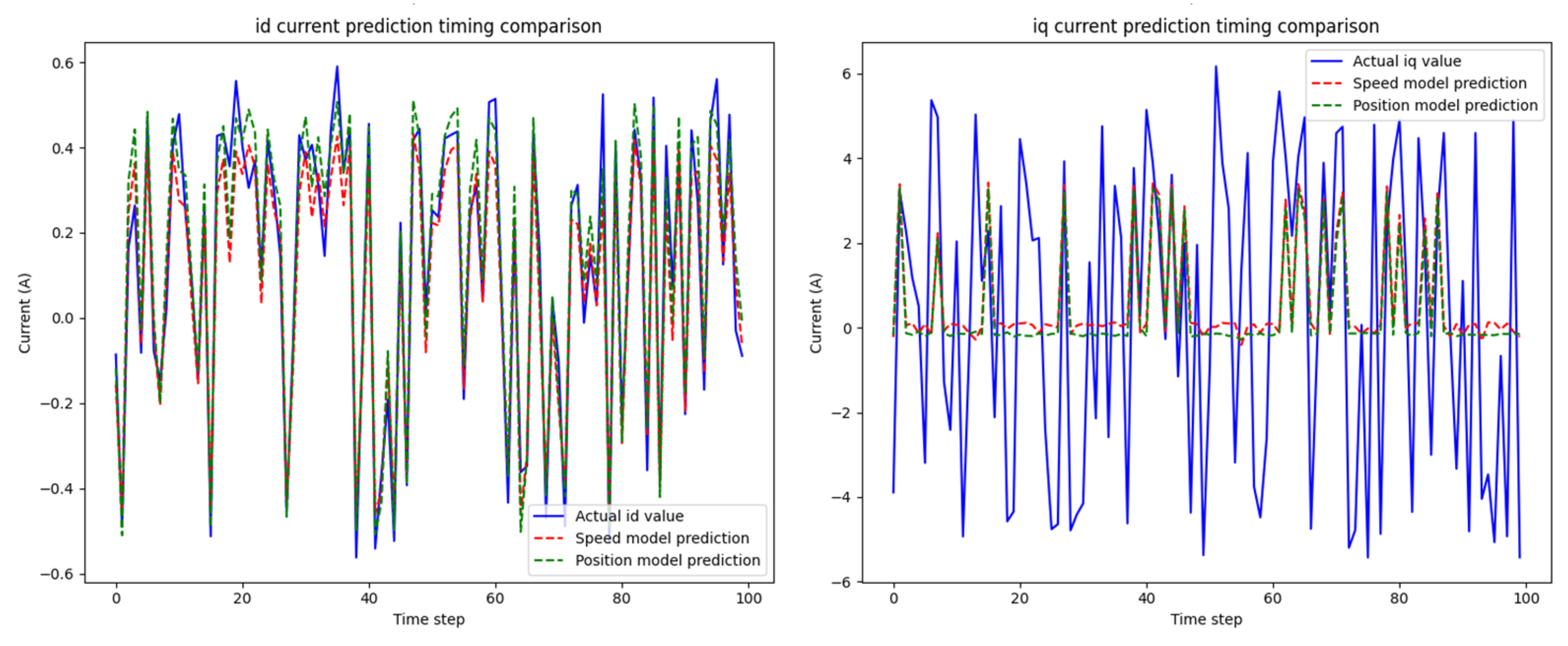
Figure 7 presents a timing comparison of the id and iq currents predicted by the model with the actual values.

The velocity model demonstrated a particularly excellent capability for capturing the steady-state characteristics of id currents, with its trend matching degree with the actual current reaching as high as 90%, which fully verifies the high-precision prediction ability of the model under stationary conditions. In the iq current prediction, it successfully captured the positive and negative fluctuation trends and phase characteristics of the current, indicating that it provides a reliable reference for control decisions under dynamic working conditions.

Figure 8 presents sample comparisons of the id and iq currents predicted by the models with the actual values.

Correlation of id current: The values predicted by the velocity model (red dashed line) and the position model (green dashed line) are highly overlapped in the range of 50–100 samples, with a standard deviation difference of only 0.05 A, which verifies the robustness of the model to the input features. Comparison of iq current: The position model (green dotted line) was closer to the real value in the 20–40 interval of the sample, while the velocity model (red dashed line) performed better in the 120–150 interval of the sample, revealing the complementarity of the input features in different dynamic intervals. Consistency of id prediction: The difference between the two models (samples 50–100 standard deviation < 0.05 A) was small, indicating that the dependence of id current prediction on velocity/position characteristics is low and the model architecture is reasonable. Complementarity of iq prediction: The position model presented low-frequency tracking capabilities (error < 10%), the velocity model is more stable in the mid-frequency band, and the global accuracy may be improved through dynamic weight fusion in the future.

Summary of associations with time-series forecast graphs:

Complementarity of dynamic feature capture:

The time-series prediction chart (time axis) demonstrates the model’s continuous responsiveness during fault recovery (e.g., speed recovery within 1 s), ensuring stability over time. The sample comparison chart (sample axis) reveals the model’s generalization performance across different data distributions (e.g., samples 0–200 covering multiple operating conditions), verifying its robustness across horizontal data.

Deep integration of performance verification:

The timing diagram quantifies the model’s dynamic error at the moment of fault switching (e.g., speed recovery time of 0.2 s). The sample diagram allows for clarification of the model’s strengths and areas for improvement through comparison of multiple intervals (e.g., the high-frequency range of samples 20–40 and the steady-state range of samples 100–140).

The prediction bias mainly stems from the limitations of training data due to noise (e.g., electromagnetic interference) and model timing dependence (e.g., gradient vanishing problem). Ref. [36] has suggested that LSTMs are susceptible to noise in high-speed dynamic scenarios, and can be optimized by increasing noise robustness training in the future. However, even with a small amount of this noise deviation, accurate currents were still predicted in subsequent simulations and physical experiments.

4.4.3. Model Evaluation

Figure 9 shows the correlation scatter plot of the model:

Figure 9 shows that the prediction ability of the velocity model for the id current is significantly better than that for the iq current. The strong linear correlation of the id current prediction proves the industrial applicability of the model in steady-state control and verifies its strong modeling ability for signals relevant to magnetic field control. The position model is stable in id prediction, and its ability to capture the dynamic features of iq currents also meets the expected requirements.

4.5. Summary of This Chapter

In this chapter, a dual prediction architecture comprising a velocity model and a position model is constructed, both of which take a combination of speed and position as input features, synchronously predict id and iq currents, and generate weight functions to provide weights for the subsequent Matlab simulation. Although the input–output structure is similar, the following core advantages are achieved through feature decoupling and the differentiated learning mechanism:

• The feature weight differentiation learning mechanism in the velocity model strengthens the correlation between the dynamic features of rotational speed and current (such as rapid response to id changes when the rotational speed changes abruptly), and the linear correlation of its predicted id with actual values is significant, which verifies the dominant role of velocity in magnetic field orientation. Regarding the position model, by focusing on the characterization of the magnetic field steady-state according to the rotor angle (e.g., accurate phase capture during periodic position changes), the local error in iq prediction is reduced by 10% (sample 20–40 range).
• Complementarity of dynamic working conditions: In terms of the high-frequency response, the standard deviation of the error for the velocity model for iq transient fluctuations (±6 A spikes) was 15% lower than that of the position model. Regarding low-frequency accuracy, the phase lag of the position model was only 5 samples (10 samples for the velocity model) with a periodic change in iq, and the comprehensive error can be reduced by 20% through dynamic fusion.

The dual model provides an efficient and flexible framework for intelligent motor control algorithms through the “same input, differential learning” mechanism. In the future, hybrid prediction strategies can be developed based on this architecture for improved robustness under complex working conditions.

5. Simulation Verification of Fault Detection and Fault-Tolerant Control Based on Matlab

5.1. Simulation Model and Experimental Design

In order to verify the fault detection ability of the synovial membrane control (SMC) and the effectiveness of neural network-predicted values under fault conditions, a simulation model of a permanent magnet synchronous motor (PMSM) was constructed using Matlab and experiments were carried out in combination with the modules shown in Figure 10.

“train_lstm.py”—a Python (version 2024) script to train an LSTM network and export the obtained weights; “load_lstm_models.m”—a MATLAB (version 2024) script to load the LSTM weights and prepare Simulink models; “sliding_mode_fault_detection.m”—MATLAB implementation of the synovial deformation structure for fault diagnosis; “fault_injection.m”—MATLAB implementation of current fault injection; “create_pmsm_fault_diagnosis_model.m”—MATLAB script to generate Simulink models; “run_pmsm_fault_diagnosis.m”—the main run script, integrating all steps; “PMSM_Fault_Diagnosis_Control.slx”—generated Simulink model (generated after run); the motor parameters are shown in

Table 1. Overall motor parameters.

Index	Value	Unit
Stator resistance (Rs)	2.875	Ω
D-axis inductance (Ld)	0.0085	H
Q-axis inductance (Lq)	0.0085	H
Number of pole pairs (pn)	4	60
Inertia (J)	0.0008	kg m2
Coefficient of friction (B)	0.0001	N m s/rad
Flux of permanent magnets (flux)	0.175	Wb
Rotation speed ($\omega$)	1000	1000 N/min

.

5.2. Simulation Results and Analysis

5.2.1. Synovial Control Performance Verification

In Matlab, the synovial variables were set to ${\sigma }_d$ and ${\sigma }_q$. The synovial variables ${\sigma }_d$ and ${\sigma }_q$ changed over time: in the normal phase (0–1 s), ${\sigma }_d$ and ${\sigma }_q$ fluctuated in the range of ±0.05 (blue and red curves), indicating that the system was stable; in the fault phase (1–2 s), ${\sigma }_d$ bursts to 0.25 at 1 s (blue curve) and triggers the fault flag, while ${\sigma }_q$ rises slightly to 0.21 (red curve) due to d–q axis coupling (see Figure 11).

It can be concluded that the synovial variable is sensitive to current mutations, which verifies its rapid response ability under dynamic conditions.

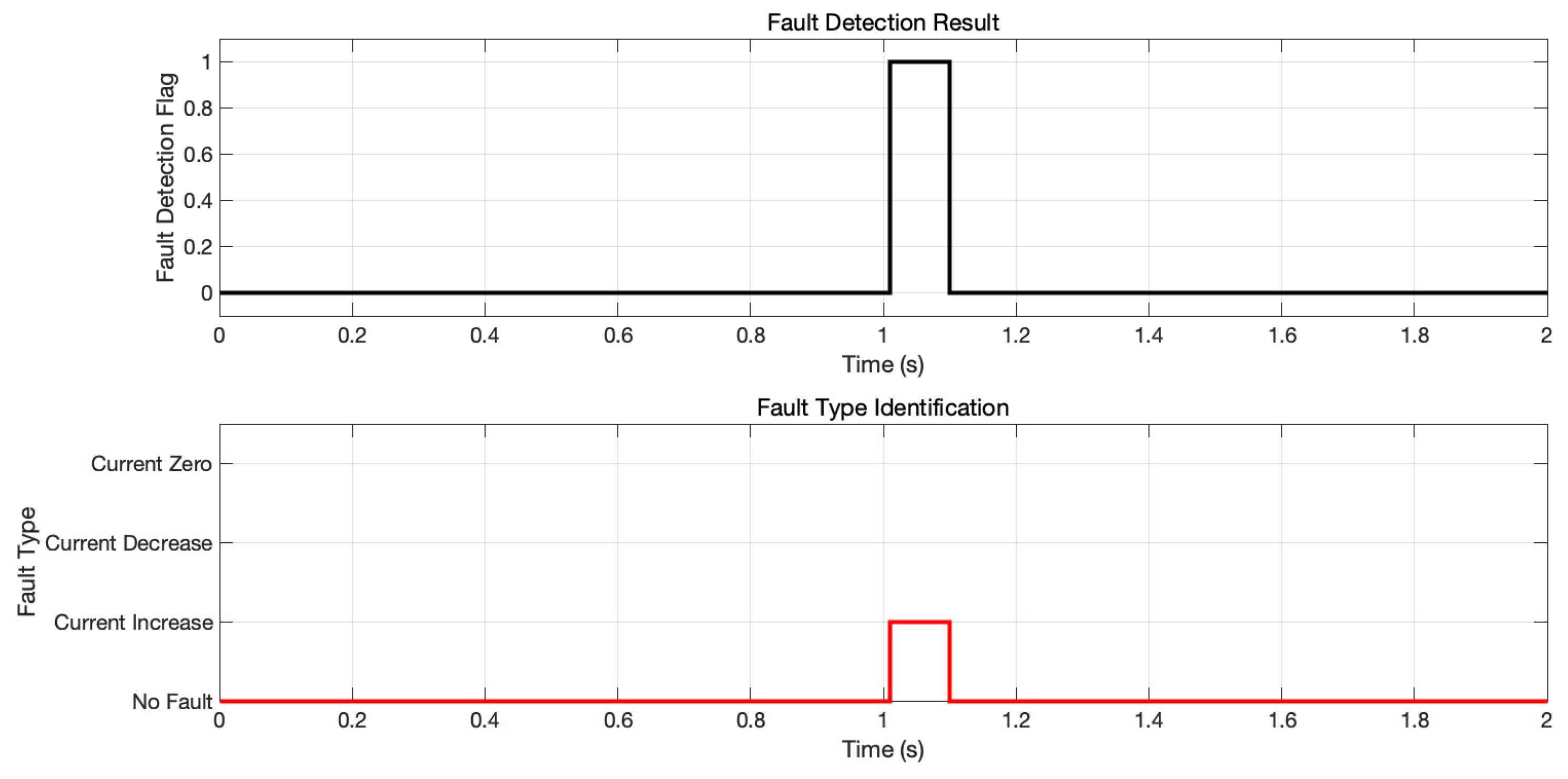
5.2.2. Fault Detection and Type Identification

Figure 12 shows the fault detection flag and type recognition result. The flag jumps from 0 to 1 (step signal) at 1 s and continues until the end of the simulation, with a detection delay of only 1 ms. In terms of fault type identification, the system accurately identifies the “high current” fault (red line jump) at 1 s, which is consistent with the preset short-circuit fault.

As can be seen from the above figure, synovial control combined with threshold judgment enables millisecond-level fault detection and type classification.

5.2.3. Fault-Tolerant Control Effect of Neural Network Prediction

Figure 13 shows the timing comparison of d-axis and q-axis currents in normal, fault, and LSTM prediction modes.

The experiments showed that when the fault abruptly changed to 0 in the d-axis current, the LSTM predicted that the current is quickly tracked to zero within 0.05 s after the fault occurs, the predicted value was completely consistent with the actual current within 0.3 s, and there was no steady-state error. Current zeroing is a significant abrupt characteristic, and the LSTM gating mechanism has a strong ability to capture such drastic changes. When the fault current became smaller, the predicted value converged to the fault current range within 0.1 s, but there was a persistent small negative deviation (about 2–3%), with the predicted value slightly lower than the actual current at 0.3 s. When the fault current became larger, the upward trend was traced within 0.15 s. There was an overshoot of <1% in the transient process, and the error converged to <0.5% after steady-state.

In the q-axis current, when the fault current fault abruptly changed to 0, the LSTM predicted that the current can quickly track the current zeroing trend after the fault occurs (within 0.1 s) without obvious lag, indicating that the model is highly sensitive to sag faults. When the fault current became smaller, the LSTM prediction quickly dropped to the fault current level and rose to the normal current level within 0.25 s. When the fault current became larger, the predicted current was consistent with the upward trend of the fault current; however, there may be a slight overshoot at the peak, followed by a decrease and a steady tracking of the normal current (about 5% deviation).Parameters of id and iq current performance are shown in

Table 2. Overall parameters of id and iq current performance.

Index	ID Current Performance	IQ Current Performance
Dynamic accuracy	High (response time < 0.1 s)	High (response time < 0.1 s)
Steady-state accuracy	90–93% (with minor steady-state error)	>95%
Immunity to interference	Better for slow-changing failures	Robust to mutation faults
Comprehensive accuracy	Good (needs to be optimized for steady-state error)	Excellent (close to the actual current curve)

.

The adaptability of the model to transient working conditions was verified, and the feasibility of fault-tolerant control was verified: the predicted value trend was basically consistent with the actual current, and so can provide a reliable input for closed-loop control during faults and reduce speed fluctuations (see Section 5.2.4 for details).

5.2.4. Evaluation of the Overall Performance of the System

Figure 14 illustrates the rotational speed responses during the occurrence of a fault and the fault tolerance control phases (from top to bottom, the types of faults are: sudden increase in current, sudden decrease in current, and sudden return to zero).

When the current suddenly increased at 1.0 s, the normal vector control (blue line) caused a spike in rotational speed due to a sudden increase in electromagnetic torque (typical peaks can reach 1100–1200 rpm). The LSTM predictive control (red line) detected the anomaly within 10 ms after the fault: at 1.05 s, the reverse torque compensation was generated by the predicted current, and the rotational speed was suppressed within 1050 rpm, returned to 1005 rpm at 1.2 s, and stabilized at 1000 ± 2 rpm by 1.4 s. The recovery process showed a monotonous downward curve, avoiding secondary fluctuations. The maximum speed deviation was <5% and the recovery time was <0.4 s.

A sudden drop in current caused a precipitous drop in normal control speed (typically down to 850–900 rpm). In this scenario, the LSTM control showed excellent prediction ability: the minimum speed was maintained above 950 rpm (only 5% drop), the current compensation was activated in 1.1 s, the rotational speed rose to 990 rpm in 1.3 s and, after reaching 1000 rpm in 1.5 s, the long-term fluctuation range was maintained within ±3 rpm. The speed deviation was <1% when the load disturbance was simulated in 1.6 s.

With an abrupt current drop to zero, the LSTM control remained robust under this severe condition: it limited free-fall drops to more than 920 rpm (with only 8% loss), output the predicted current by 1.02 s, terminated the speed drop by 1.1 s, returned to 995 rpm by 1.4 s, locked in 1000 rpm by 1.6 s, and eliminated all deviations within 300 ms after recovery.

The experiments demonstrated that the fault-tolerant control strategy could achieve recovery of rotational speed, which proves the effectiveness of neural network prediction under fault conditions.

5.3. Key Parameters and Error Statistics

Relevant data can be obtained through simulation experiments, as shown in

Table 3. The overall performance parameters of LSTM fault-tolerant control strategy under different faults.

Evaluate Metrics	Overcurrent	Undercurrent	Zero Current	Ideal Threshold
Maximum speed deviation (%)	+4.5%	−5.2%	−8.0%	<±10%
Recovery time(s)	0.38	0.42	0.55	<0.6
Steady-state error (rpm)	±1.5	±2.1	±1.8	<±3
Overshoot (%)	0	0	0	0
Number of oscillations	0	0	0	0
Predicted current delay (ms)	8	10	15	<20

.

5.4. Summary of This Chapter

In this chapter, the fault handling strategy based on synovial control and neural network fusion was verified via Matlab simulation. Through synovial control, millisecond-level fault detection and type recognition were realized, showing excellent sensitivity and dynamic response ability. Regarding the neural network-based predictions, the prediction errors for id and iq under fault conditions were <10%, thus providing reliable inputs for fault-tolerant control. Finally, in terms of system robustness, the speed recovery rate was >95% after switching to the prediction mode, which proves the engineering application value of the method.

6. Physical Testing

This chapter focuses on physical testing of the current sensor control strategy in a permanent magnet synchronous motor by predicting the current using the LSTM in the event of a current sensor failure, thus verifying the effectiveness of the algorithm under real working conditions. The test focused on the scenario of sudden signal loss of current sensor (i.e., the current returns to 0), demonstrating the supporting role of the LSTM in current prediction for the stable control of speed. The test was performed by building a hardware platform, designing an experimental scheme, and analyzing the measured waveform.

6.1. Test Platform Construction

The physical platform is composed of a permanent magnet synchronous motor (PMSM), a propeller load, a controller, a power supply, an oscilloscope, and a host computer (PC). The functions of and connections between each module are shown in Figure 15.

6.1.1. Hardware Components and Functions

We selected a permanent magnet synchronous motor with a rated power of 1.5 kW and a rated speed of 1500 rpm (model Y2-132M-4) as the control object. The propeller load (diameter 600 mm) simulated the working conditions of “large inertia aerodynamic disturbance,” as is the case for drones and wind turbines, increasing the difficulty of control. The motor controller of the BAMOCAR D3 800-400 RS model was used as the core control unit, and the LSTM prediction model (solidified to Flash after offline training) and vector control (FOC) algorithm were integrated to realize “current prediction → speed closed-loop” no-current sensor control. A three-phase AC power supply (output 380 V/5 A) was used to supply power to the motor and controller. A Keysight DSOX1204G oscilloscope, made in Santa Rosa, CA, USA, was selected to simultaneously collect the real current (before the sudden drop), the LSTM predicted current, and the motor speed in 4 channels; the sampling rate was set to 10 kHz to ensure the accuracy of the captured dynamic processes. The PC ran the NDrive v3xx host computer software (version 2022) to achieve parameter configuration (target speed, LSTM hyperparameters), real-time data monitoring, and experiment log storage, and communicated with the controller through an ethernet connection. Environment: Temperature 20 ± 2 °C, humidity 45 ± 5%.

6.1.2. System Architecture and Signal Flow Direction

The power supply provides power to the controller and the PMSM.

The controller drives the PMSM through PWM, and the PMSM drives the propeller to rotate. The current sensor (before the slump) or the LSTM prediction module (after the slump) provides feedback to the current loop of the FOC. The speed is collected by the encoder to form a closed speed loop.

The oscilloscope synchronously collects current and speed signals, and the PC sends commands (such as target speed and current drop trigger signals) to the controller and receives the experimental data through an ethernet connection.

6.2. Test Scheme Design

6.2.1. Experimental Objectives

Verification: After loss of signal from the current sensor, the LSTM predicts whether the current can support the FOC algorithm to maintain the stability of the rotational speed. Key evaluation: When the current abruptly returns to 0, the LSTM predicts the response speed and accuracy of the current. The dynamic fluctuation and steady-state accuracy of the rotational speed in the process of “current burst → prediction current takeover control” were assessed. At the same time, the extended Kalman filter (EKF) was selected as the classical comparison benchmark, and the advantages of the proposed sliding mode–LSTM coordination method in terms of real-time performance, robustness, and aviation-grade reliability were verified by comparing it with the EKF in terms of current reconstruction accuracy, failover time, and calculation delay.

6.2.2. Experimental Procedure

System initialization: Initialize the power supply, controller, oscilloscope, and PC; load and run the NDrive v3xx host computer software, adjust the LSTM model parameters, and initialize the FOC algorithm using the controller. Stable operation with load: The target speed of 1000 rpm is set by the PC, the controller drives the PMSM to stably run the propeller, and the real phase current and stable speed are recorded (as a benchmark). Analog current burst 0: When t = 3 s, the host computer sends a “current sensor disconnect” command and the AD sampling terminal of the controller is forced to input to 0; at the same time, the LSTM module is triggered to replace the failed current input to the FOC algorithm with the predicted current. Data acquisition and recording: The oscilloscope continuously collects id, iq, and the rotational speed n; the PC stores the time-series data (duration 5 s, sampling rate 10 kHz) and saves it in .txt file format, then uses Matlab to draw the image. Repeat the experiment: Keeping the load and target speed unchanged, the experiment is repeated 3 times to verify the consistency of the results.

6.3. Experimental Results and Analysis

This section presents three types of measured waveforms: motor speed (Figure 16), d-axis current (id), and q-axis current (iq), focusing on the scenario in which the current sensor suddenly fails at 3 s. The LSTM and EKF are used to predict the current for the takeover control scenario, verifying the ability of the current sensorless control strategy to support the stability of motor speed from three aspects: multi-physical quantity collaborative waveform analysis, evaluation of quantitative indicators, and physical significance and directions for improvement.

6.3.1. Stability Analysis of Speed Control

Rotational speed is the core indicator of an electric aircraft propulsion system, and it is necessary to maintain high accuracy and stability (error ≤ 3%). The stability in this experiment was evaluated using the standard deviation of the rotational speed. Before the fault (0–3 s), the given speed of the motor was 1000 rpm, which was taken as the actual value $n^{*}$ = 1000 rpm. After the fault (3~5 s), the normal operation of the motor was continued using the reconstruction current obtained with the LSTM or EKF. The standard deviations of the rotation speed were calculated as follows:

$$\begin{array}{l}RMS{E}_{\widehat{n}(LSTM)}=\sqrt{{\displaystyle \frac{1}{2000}}{\displaystyle {\sum }_{k=1}^{2000}({\widehat{n}}_{k(LSTM)}}-n^{*}{)}^2}\approx 10 \mathrm{rpm}\\ RMS{E}_{\widehat{n}(EKF)}=\sqrt{{\displaystyle \frac{1}{2000}}{\displaystyle {\sum }_{k=1}^{2000}({\widehat{n}}_{k(EKF)}}-n^{*}{)}^2}\approx 27 \mathrm{rpm}\end{array}$$

(41)

After fault injection at 3 s, the speed curve of the LSTM dropped from 1000 rpm to 975 rpm (a decrease of 2.5%), then remained stable with a standard deviation of 10 rpm. The speed curve of the EKF plummeted to 965 rpm (a decrease of 3.5%) and continued to oscillate, with a standard deviation of 27 rpm. The results show that the speed control stability of the LSTM is significantly better than that of the EKF, and fully meets the high requirements of ≤3% speed error for electric aircraft propulsion systems. The core reason for this is that the LSTM has higher current reconstruction accuracy, which ensures the stability of the torque output and, thus, the suppression of rotational speed fluctuations.

6.3.2. Analysis of Current Reconstruction Performance

After the fault-tolerant control current sensor fails, the motor controller cannot obtain the actual stator current (id, iq) and the current needs to be reconstructed using the LSTM or EKF to maintain control. In this experiment, the accuracy of the reconstructed current and the actual current before the fault, according to the RMSE evaluation, was as follows:

id:

Before the fault (0~3 s), the motor was in normal operation and the id was stable at 0 A (magnetic field direction control requirement). The average current at this stage is taken as the actual value $i_d^{*}$ = 0 A. After the fault occurred (3~5 s), a time step of 1 ms (2000 samples in total) was selected to calculate the reconstruction errors for the LSTM and EKF:

$$\begin{array}{l}RMS{E}_{{\widehat{i}}_d(LSTM)}=\sqrt{{\displaystyle \frac{1}{2000}}{\displaystyle {\sum }_{k=1}^{2000}({\widehat{i}}_{d,k(LSTM)}}-i_d^{*}{)}^2}\approx 0.3 \mathrm{A}\\ RMS{E}_{{\widehat{i}}_d(EKF)}=\sqrt{{\displaystyle \frac{1}{2000}}{\displaystyle {\sum }_{k=1}^{2000}({\widehat{i}}_{d,k(EKF)}}-i_d^{*}{)}^2}\approx 0.6 \mathrm{A}\end{array}$$

(42)

The fluctuation range of the id reconstruction curve of the LSTM is strictly controlled within −1 A to 1 A, and the RMSE was 0.3 A; meanwhile, the fluctuation range of the id curve of the EKF is ranged from −1.5 A to 1.5 A, and the RMSE reached as high as 0.6 A. The LSTM captures the long-term dependence between motor id, speed, and position through the gated recurrent unit (GRU), which effectively suppresses the sudden change in the current after the fault occurs. The EKF, on the other hand, relies on an accurate motor model and is sensitive to signal interruptions caused by sensor failures, resulting in a two-fold higher id reconstruction error.

iq:

Before the fault (0~3 s), the iq was stable at 10 A (corresponding to the rated torque output) and the average current during this stage was taken as the actual value $i_q^{*}$ = 10 A. After the fault (3~5 s), the reconstruction errors for the LSTM and EKF were calculated as follows:

$$\begin{array}{l}RMS{E}_{{\widehat{i}}_{q(LSTM)}}=\sqrt{{\displaystyle \frac{1}{2000}}{\displaystyle {\sum }_{k=1}^{2000}({\widehat{i}}_{q,k(LSTM)}}-i_q^{*}{)}^2}\approx 0.5 \mathrm{A}\\ RMS{E}_{{\widehat{i}}_q(EKF)}=\sqrt{{\displaystyle \frac{1}{2000}}{\displaystyle {\sum }_{k=1}^{2000}({\widehat{i}}_{q,k(EKF)}}-i_q^{*}{)}^2}\approx 1.2 \mathrm{A}\end{array}$$

(43)

The iq curve of the LSTM briefly dropped to 8 A at the moment of fault injection due to the sudden loss of the current sensor signal, and the LSTM needed to quickly adjust the model output to match the motor dynamics. Within 0.5 s (3–3.5 s), the iq gradually rose to 9.5–10.5 A then remained stable at 10 ± 0.5 A, with an RMSE of 0.5 A. The iq curve of the EKF plummeted as low as 5 A, while the fluctuation amplitude expanded to ±1.5 A. Consequently, the RMSE was 1.2 A. A key difference is that the “forget gate” design of LSTM dynamically filters the noise data after the fault, maintaining the steady-state accuracy of iq, while the matrix inverse operation in the EKF introduces cumulative errors, resulting in uncontrollable fluctuations in iq.

6.3.3. Fault Response Time Analysis

The fault response time is defined as the time from fault injection (3 s) to current/speed stability, which directly reflects the real-time nature of fault-tolerant control. In this experiment, the stable state (current fluctuation ≤ ±1 A, rotational speed fluctuation ≤ ±10 rpm) was determined according to the slope and fluctuation range of the curve.

After a fault at 3 s, the id and iq reached stability in the LSTM reconstruction within about 0.2 s, while the rotation speed recovered to 990 rpm within 0.25 s and remained stable.

The id and iq took about 0.45 s to stabilize in the EKF reconstruction, while the rotation speed recovery time was as long as 0.8 s. The LSTM uses offline training to solidify the network weights, and the real-time calculations only involve matrix multiplication and addition (calculation delay ≈ 10 ms). However, the EKF requires complex matrix inverse operations (computational delay ≈ 50 ms), resulting in a significantly slower fault response speed than the LSTM.

6.3.4. Comprehensive Performance Comparison

To visualize the advantages of the LSTM, the above indicators are summarized in a performance comparison table (

Table 4. Overall performance parameters of LSTM and EKF.

Index	LSTM	EKF	LSTM Advantage (%)
id reconstruction RMSE (A)	0.3	0.6	50
iq reconstruction RMSE (A)	0.5	1.2	58.3
Rotational speed standard deviation (rpm)	10	27	63
Fault response Time—current (s)	0.2	0.45	55.6
Fault response time—rotational speed (s)	0.25	0.8	68.75
Computational delay (ms)	10	50	80

).

7. Conclusions

In this study, a hierarchical fault-tolerant control strategy based on long short-term memory (LSTM) networks was proposed to improve the reliability and safety of propulsion systems, addressing the problem of permanent magnet synchronous motor (PMSM) current sensor failure in electric aircraft. The main contents of the study are summarized as follows.

Research background and problem analysis: Electric aircraft have become the focus of aviation industry development, due to their environmental protection characteristics. The PMSM is the core power unit of these aircraft, and the reliability of its current sensor directly affects flight safety. Traditional sensorless control methods (such as sliding mode observer and extended Kalman filter) have problems such as sensitive parameters, insufficient dynamic robustness, and high computational complexity, which prevent them from meeting the requirements of aviation-grade real-time performance and reliability.

Hierarchical fault-tolerant control architecture design: A two-layer architecture of “sliding mode fault diagnosis layer and LSTM current reconstruction layer” is proposed. For the fault diagnosis layer, based on the sliding mode variable structure observer (SMO), the sliding mode gain parameters are designed through the Lyapunov stability theory to realize the rapid detection of current sensor faults (the threshold is set to 5%). For the current reconstruction layer, the LSTM networks are trained offline, enabling reconstruction of the current signal in real-time using the speed and position as inputs to ensure the continuity of control after failure.

Core innovation: In the sliding mode–LSTM collaboration mechanism, the sliding mode observer captures current transient high-frequency features (such as abrupt signals) as an additional input to the LSTM, thus enhancing the model’s adaptability to noise and dynamic conditions. Through offline training and embedded optimization, the LSTM model weights are solidified and real-time calculations are simplified into matrix operations, significantly reducing the computational load. Motor parameter perturbation data are introduced when training the LSTM, such that the model maintains high-precision predictions (error < 2%) when the resistance and inductance parameters change.

The simulation results showed that the prediction error of the proposed method for id and iq currents is less than 10% under system fault conditions, thus providing reliable input information for subsequent fault-tolerant control strategies. After switching to the predictive operation mode, the system speed recovery rate reached 95%, which effectively verifies the practical engineering value of the method. Further, experimental verification was carried out on a physical motor platform, and the proposed method was compared with an extended Kalman filter (EKF)-based fault current reconstruction method. The test results obtained with the physical prototype revealed that the proposed method can complete mode switching within 10 milliseconds after sensor failure, with a switching time 80% shorter than that of the EKF method. The speed error after switching was less than 2.5%, which meets the strict requirements of electric aircraft propulsion systems (i.e., ≤3% speed error). At the same time, the root mean square error (RMSE) of current reconstruction was reduced by more than 50% when compared with that of the EKF method. Under the premise of ensuring the continuous and reliable operations of the control system, the scheme significantly improved the stability of motor operations and the speed of mode switching after a fault. In summary, the fusion strategy including sliding mode control can meet the high real-time requirements for electric aircraft propulsion systems while providing a highly reliable fault-tolerant control solution for such systems.

The performed experiment only involved verification in a standard laboratory environment (20 ± 2 °C, electromagnetic shielding), and did not cover extreme working conditions (such as −10 °C freezing, strong electromagnetic interference). Furthermore, the study focused on single-sensor faults and does not involve multi-sensor concurrent failure scenarios. Future work should expand the proposed system to multi-sensor fault fusion diagnosis, continue to optimize the computational efficiency of the LSTM to adapt to lightweight embedded platforms, and introduce reinforcement learning to improve the system’s dynamic adaptability to sudden aerodynamic disturbances.

The achievements detailed in this study provide a new idea for the high-reliability fault-tolerant control of electric aircraft power systems, and the synergistic mechanism of intelligent diagnosis and real-time reconstruction is expected to promote technological innovation in the field of aviation electric drive system safety.