
Mission Planning for UAV Swarm with Aircraft Carrier Delivery: A Decoupled Framework

 ,
, 
 ,
, 
Abstract
1. Introduction
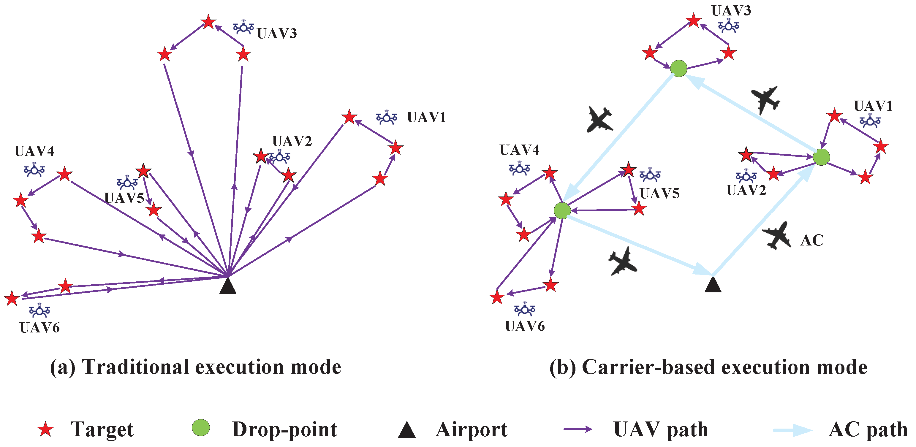
1.1. Background
1.2. Literature Review
1.3. Motivation and Contribution
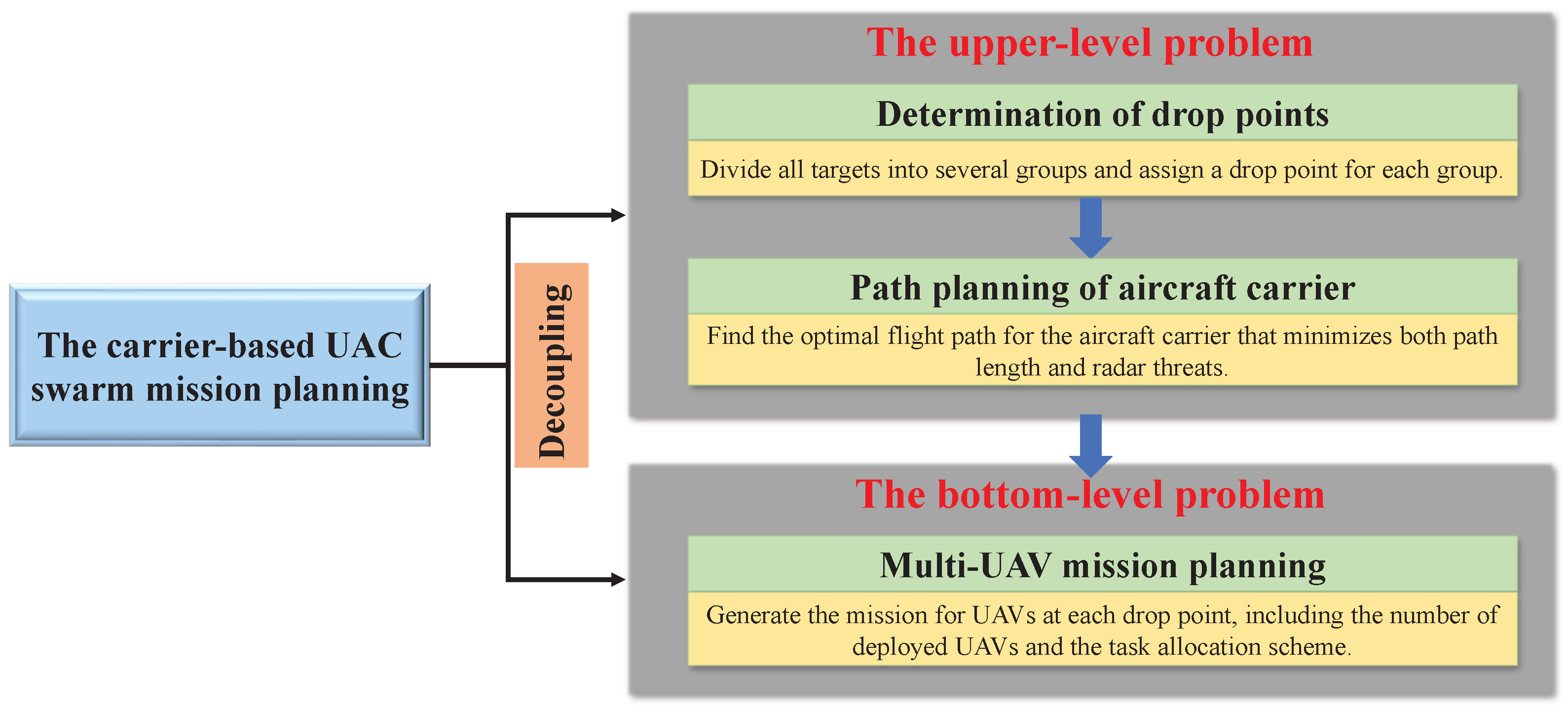
- We design a decoupled planning framework that decomposes the carrier-based UAV swarm mission planning problem into a two-level planning process. This decoupled architecture enhances the adaptability and extensibility of the planning process, making it capable of addressing coordinated planning in complex large-scale scenarios. Additionally, to the best of our knowledge, this paper is the first to propose and investigate the carrier-based UAV swarm mission planning problem.
- For the upper-level problem, we develop a selection method based on the principles of distance and threat minimization to address the DP determination problem. Then, we propose a discrete genetic algorithm incorporating an improved A* algorithm (DGAIIA) to plan the global path of AC. In the DGAIIA method, a variant of the single traveler problem is formulated, which considers radar threats and no-fly zones.
- For the bottom-level problem, we establish the multi-objective optimization model for cooperative mission planning of multiple UAVs, with time cost and UAV utilization as the optimization objective. To solve this problem, we propose an improved differential evolution algorithm with a market mechanism (IDEMM), which features a dual switching search strategy and a neighborhood-first buying-and-selling mechanism.
- Simulation experiments demonstrate that the carrier-based UAV swarm mission planning problem can be efficiently solved by the DGAIIA and IDEMM algorithms. Furthermore, the IDEMM algorithm is superior to other benchmark algorithms in terms of convergence performance. Our proposed framework can be easily extended to other mission scenarios involving coordinated planning of multiple types of platforms.
1.4. Organization
2. System Model
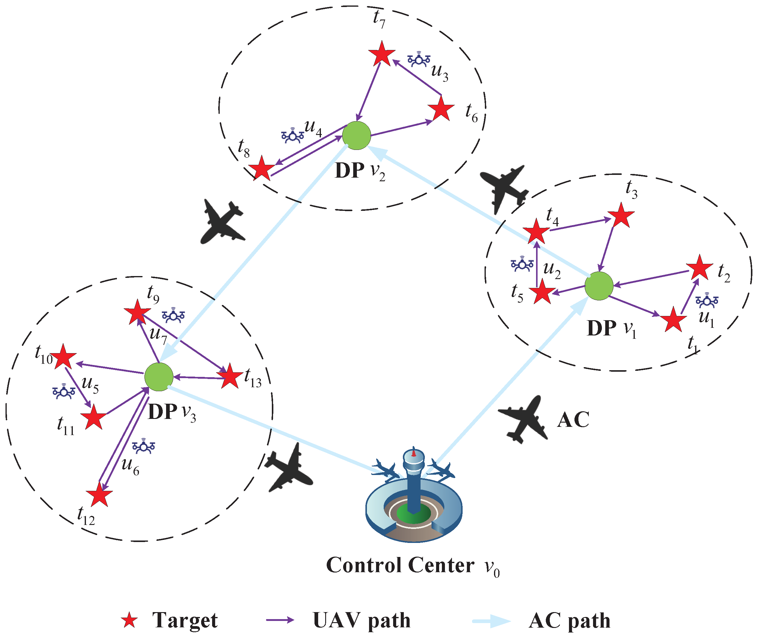
2.1. An Overview of the Carrier-Based UAV Swarm Mission Planning
2.2. The Path Planning Model of AC
2.3. The Task Assignment Model of UAVs
3. Algorithm Design
3.1. DP Determination Combined with Distance Clustering
- (1)
- Target Clustering
- (2)
- Optimization of the Cluster Center
- (3)
- Determination of the DPs
| Algorithm 1 The DP Determination Algorithm |
Input: The position of targets and the number of DPs. Output: The classification of target and the position of DPs. 1: Initialize cluster center . ****************************Clustering of targets **************************** 2: For do 3: Cluster targets according to Equation (15). 4: End For **********************Optimization of the Cluster Center********************** 5: For do 6: Calculate . 7: For do 8: Calculate . 9: If do 10: unchanged. 11: Else 12: . 13: End If 14: End For 15: End For ****************************Determination of DPs*************************** 16: For do 17: The DP is determined according to Equation (17). 18: End For 19: Return , . |
3.2. AC Path Planning Combined with Improved Genetic and A* Algorithm
- (1)
- The Selection Operation
- (2)
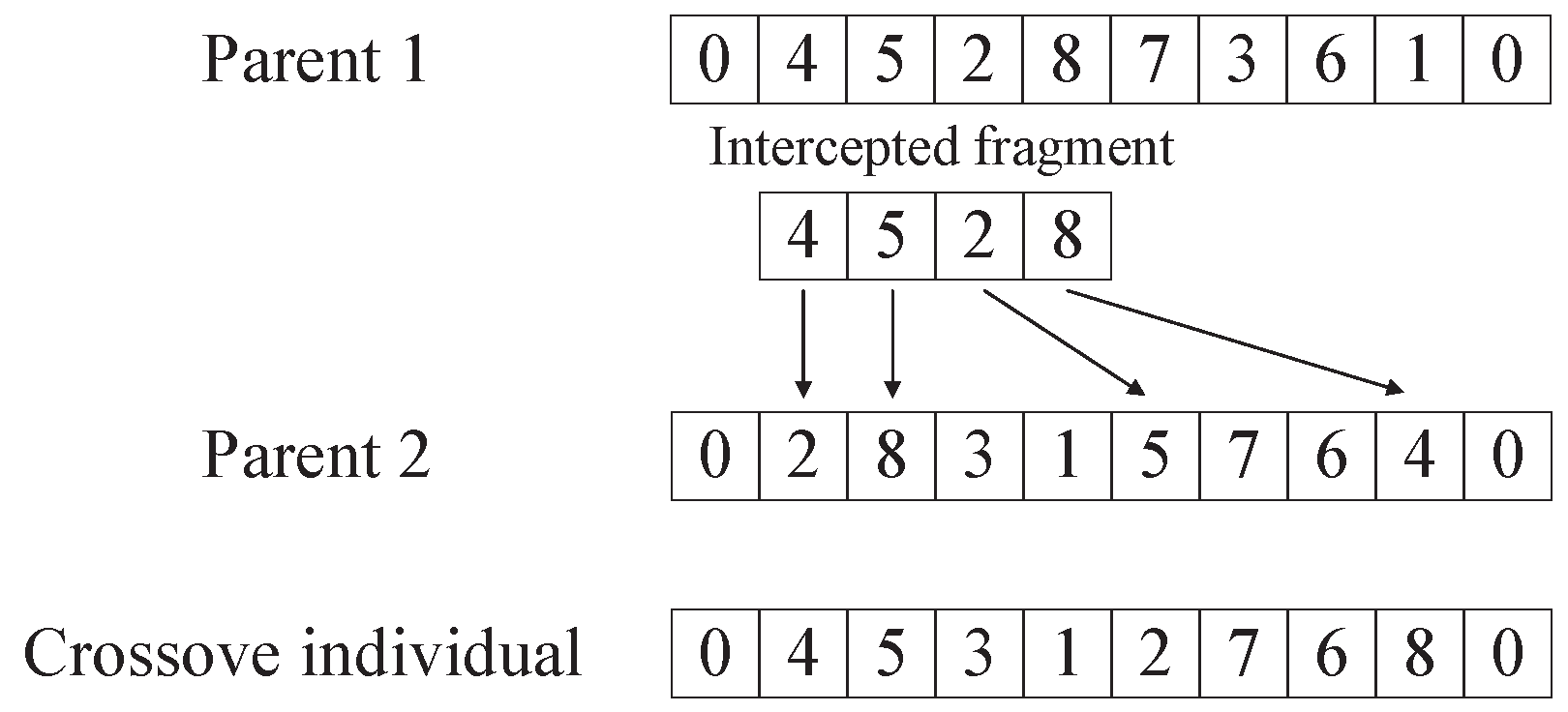
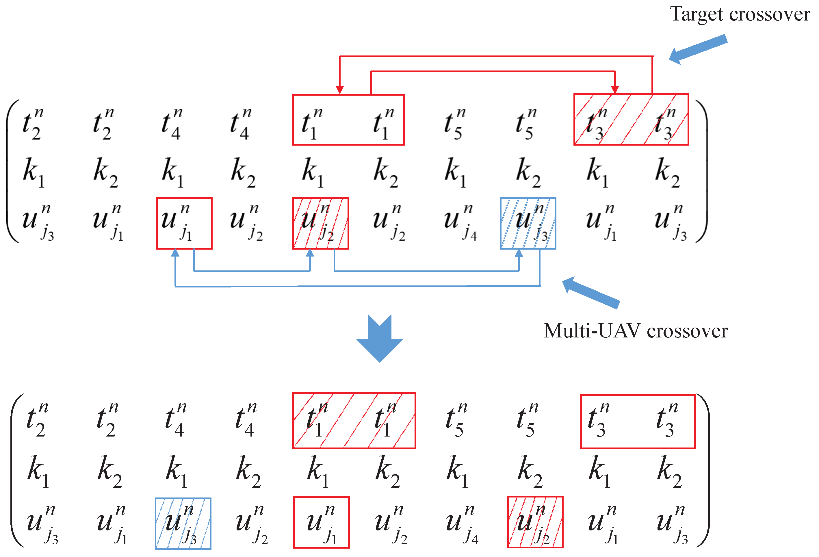
- The Crossover Operation
- (3)
- The Mutation Operation
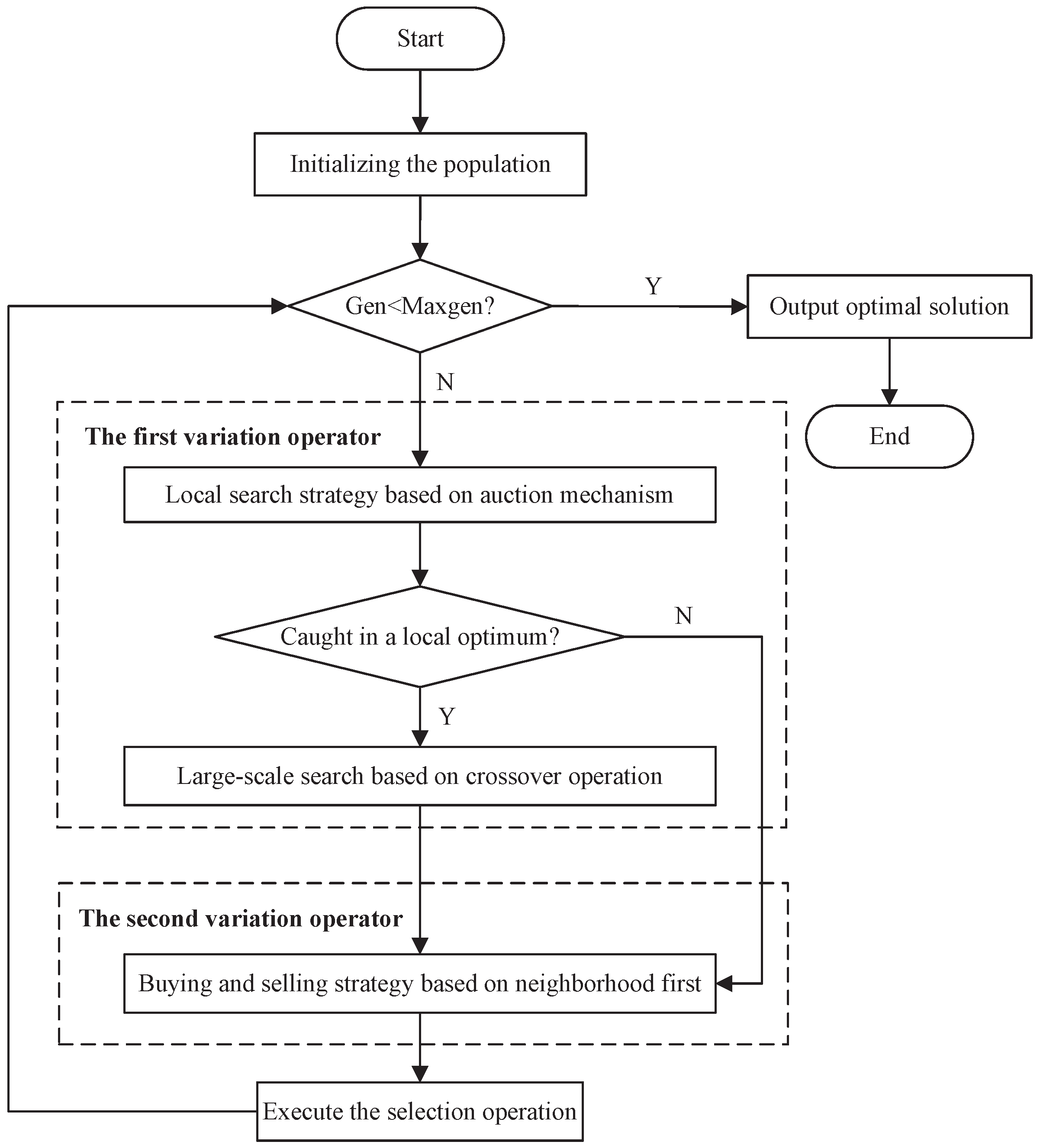
3.3. The Multi-UAV Cooperative Mission Planning Combined with Improved Differential Evolution Algorithm
| Algorithm 2 The AC path planning algorithm |
Input: Location of DPs, radars, and no-fly zones; the number of DPs N; population size ; maximum iteration ; mutation rate . Output: The DP association decision , and the flight path of AC. 1: Initialize the population based on the improved A* algorithm. 2: For do 3: Let . 4: While do 5: Execute the selection operation. 6: Execute the crossover operation. 7: If do 8: Execute the mutation operation. 9: End If 10: . 11: End While 12: Record the optimal individual in the i-th generation. 13: End For 14: Return . |
- (1)
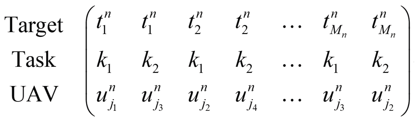
- Task Assignment Scheme Coding
- (2)
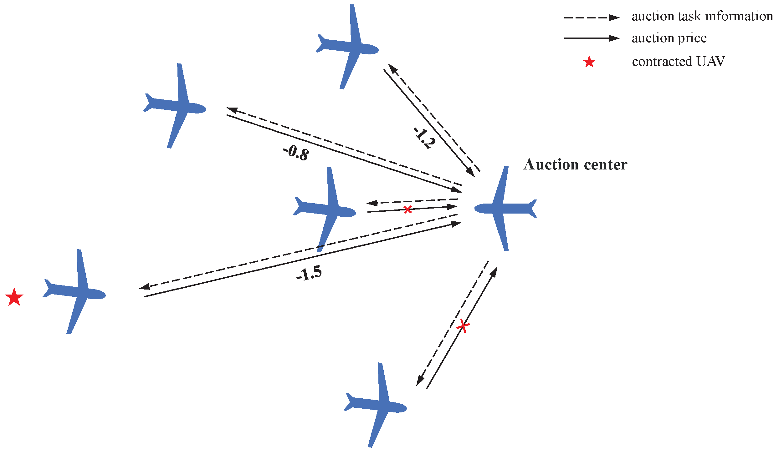
- The First Variation Operator
- (3)
- The Second Variation Operator
4. Simulation and Analysis
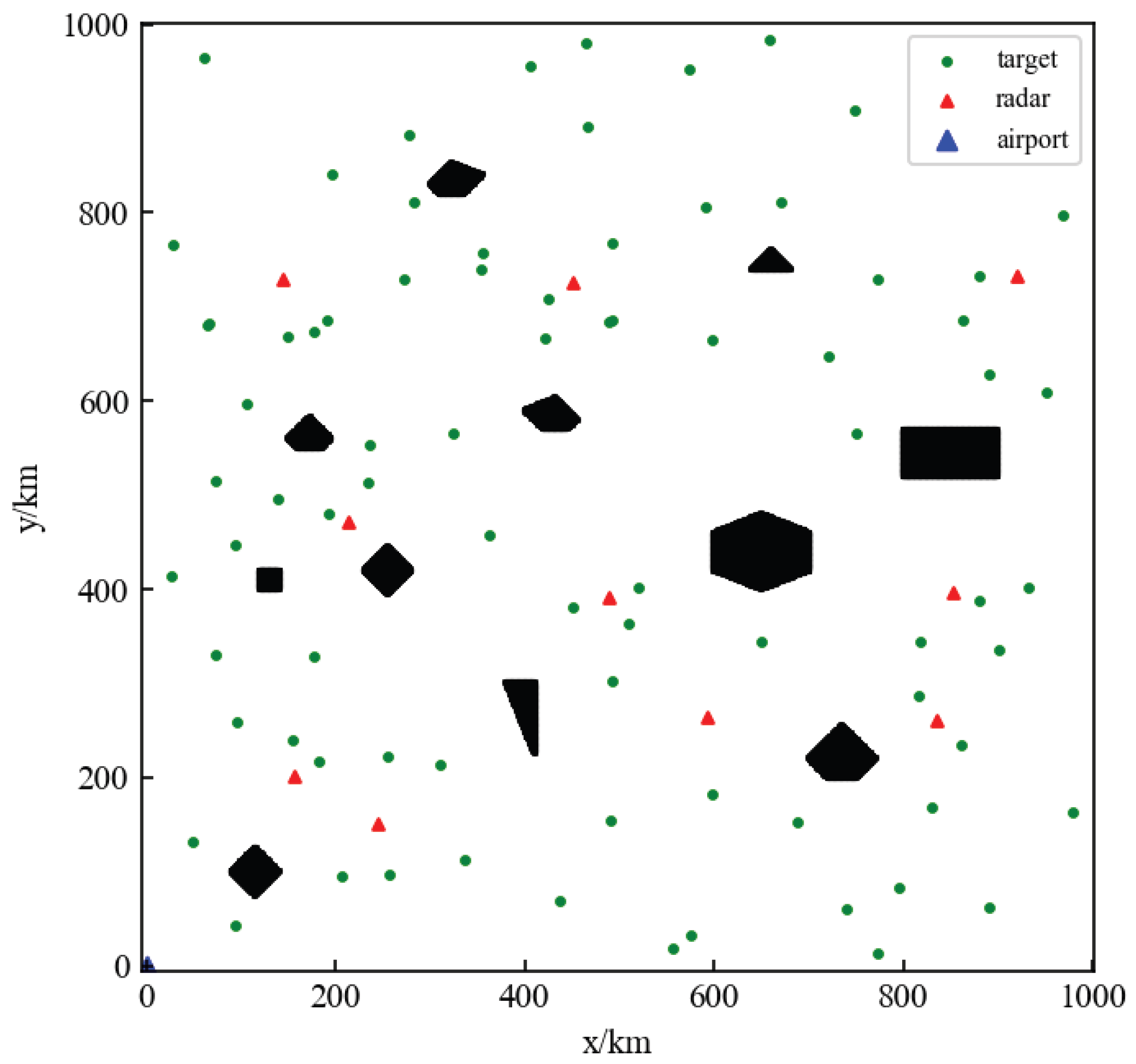
4.1. Environment Settings
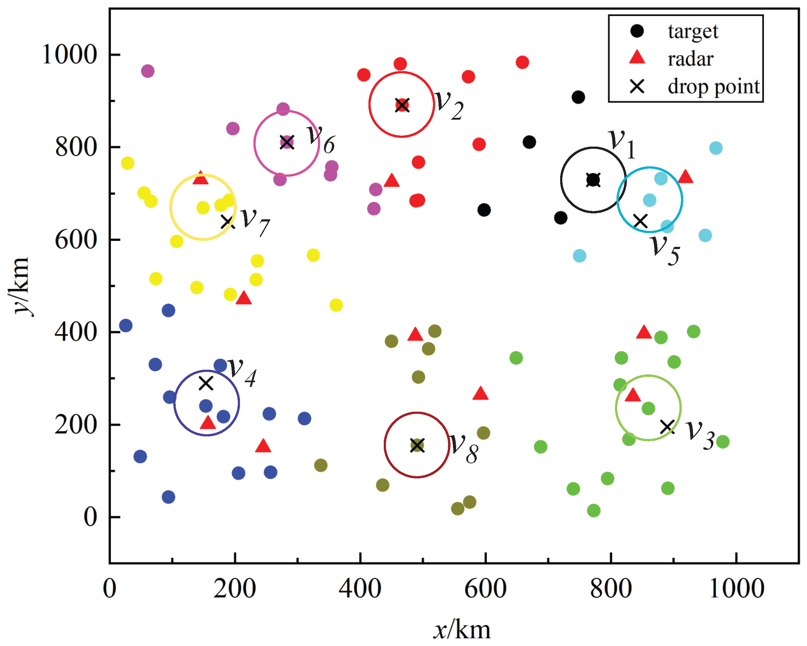
4.2. The Location Determination of DPs
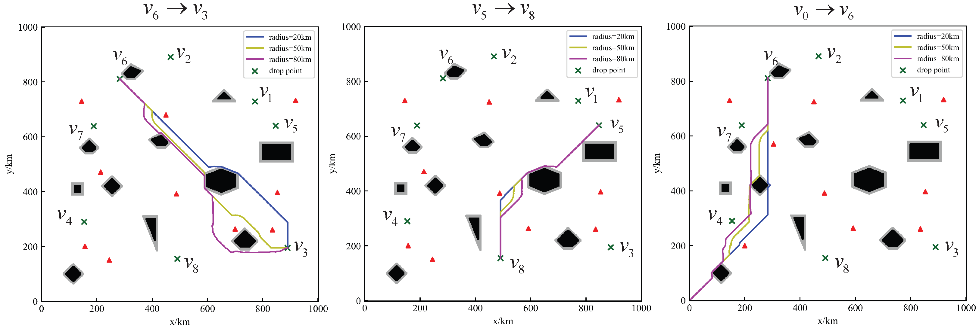
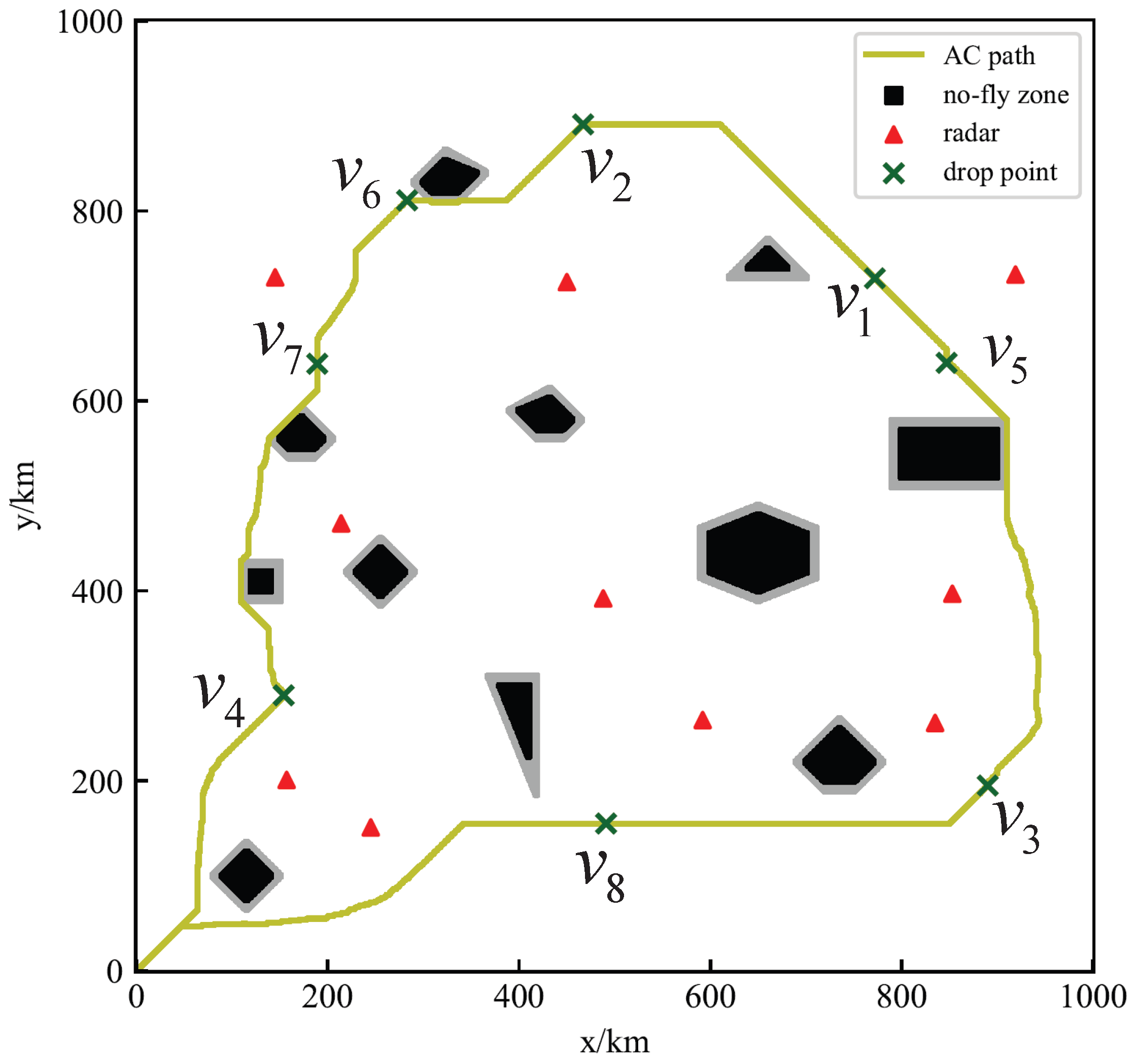
4.3. The AC Path Planning
- (1)
- The Path Planning between any two DPs
- (2)
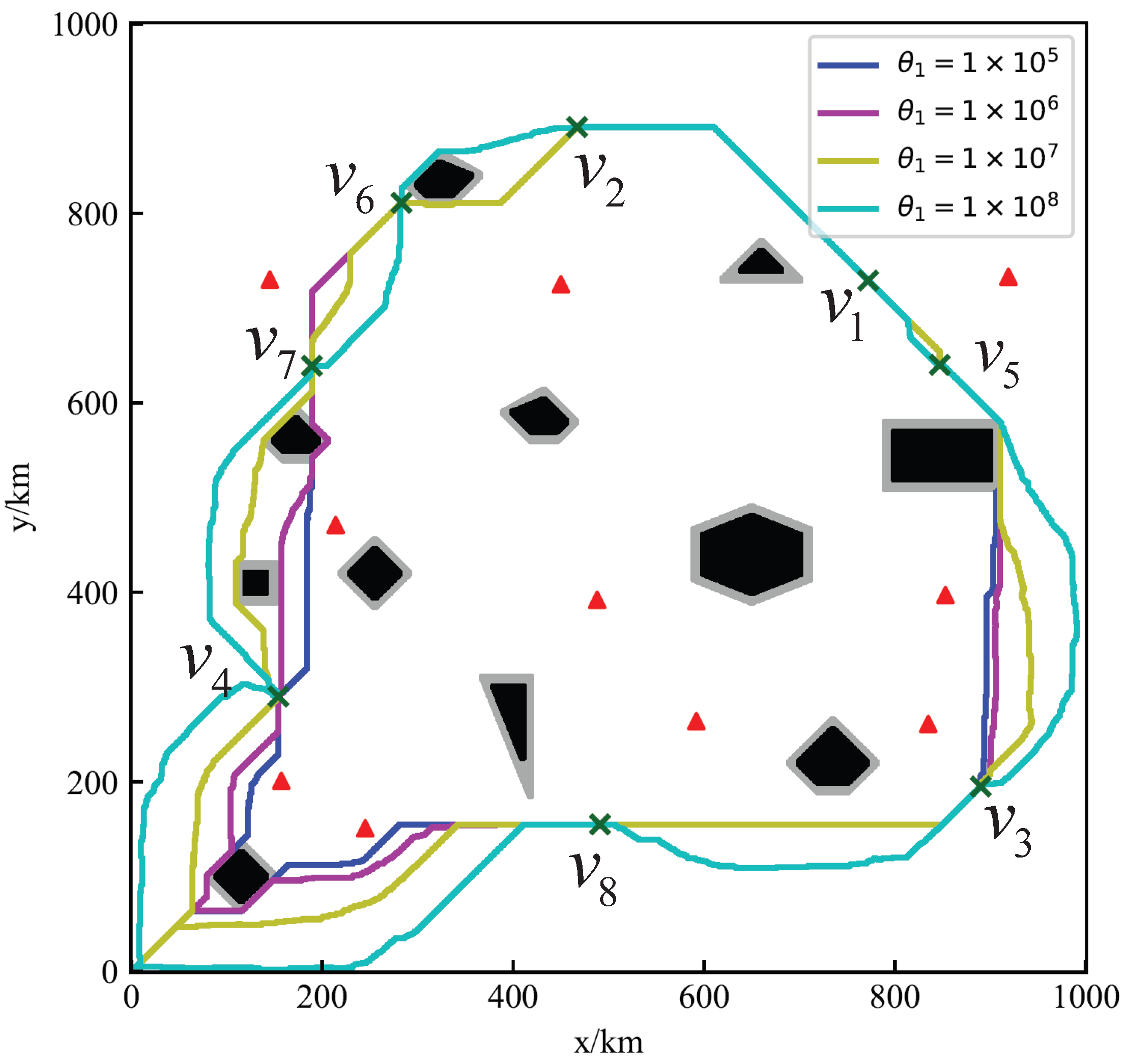
- The Overall Path Planning of AC
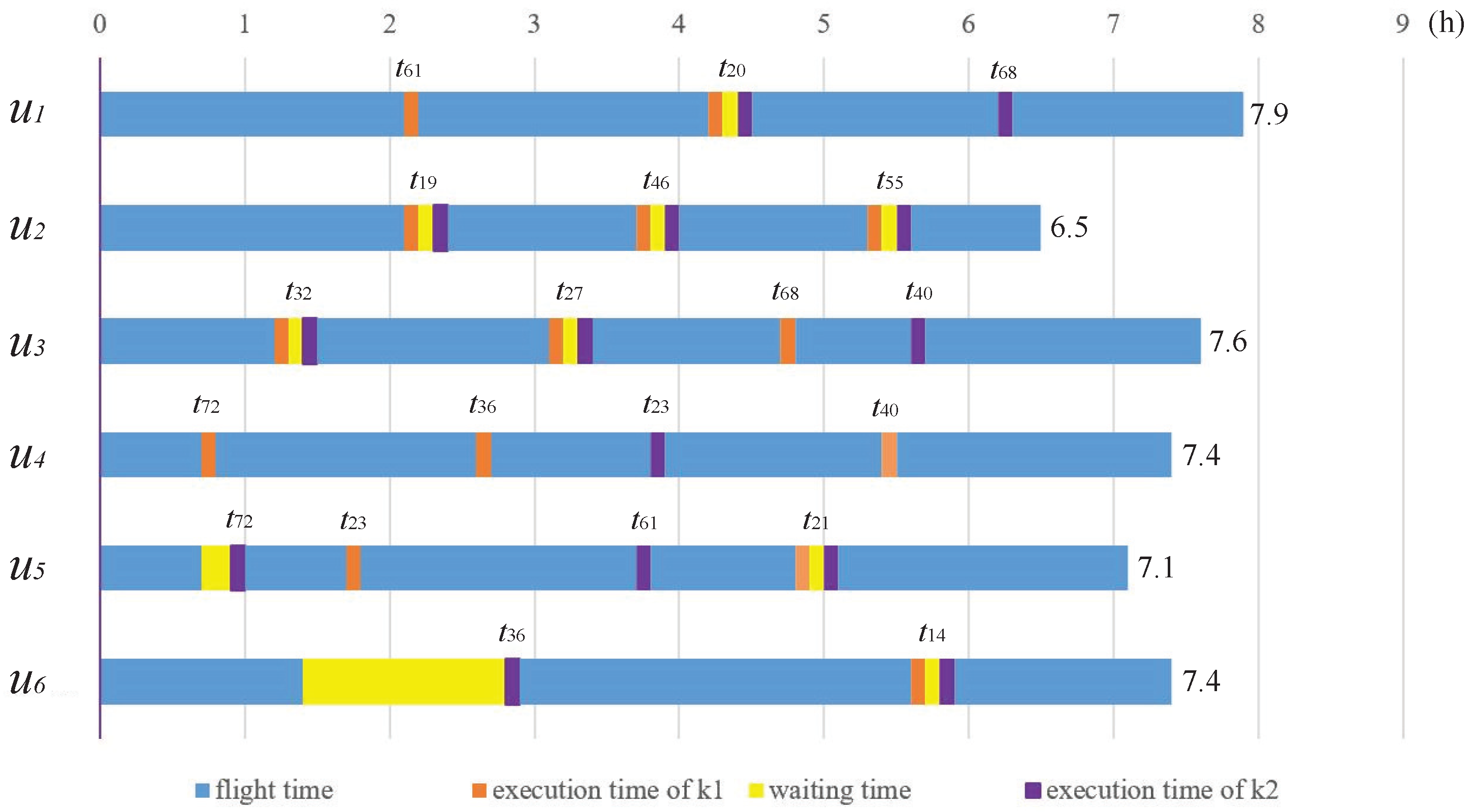
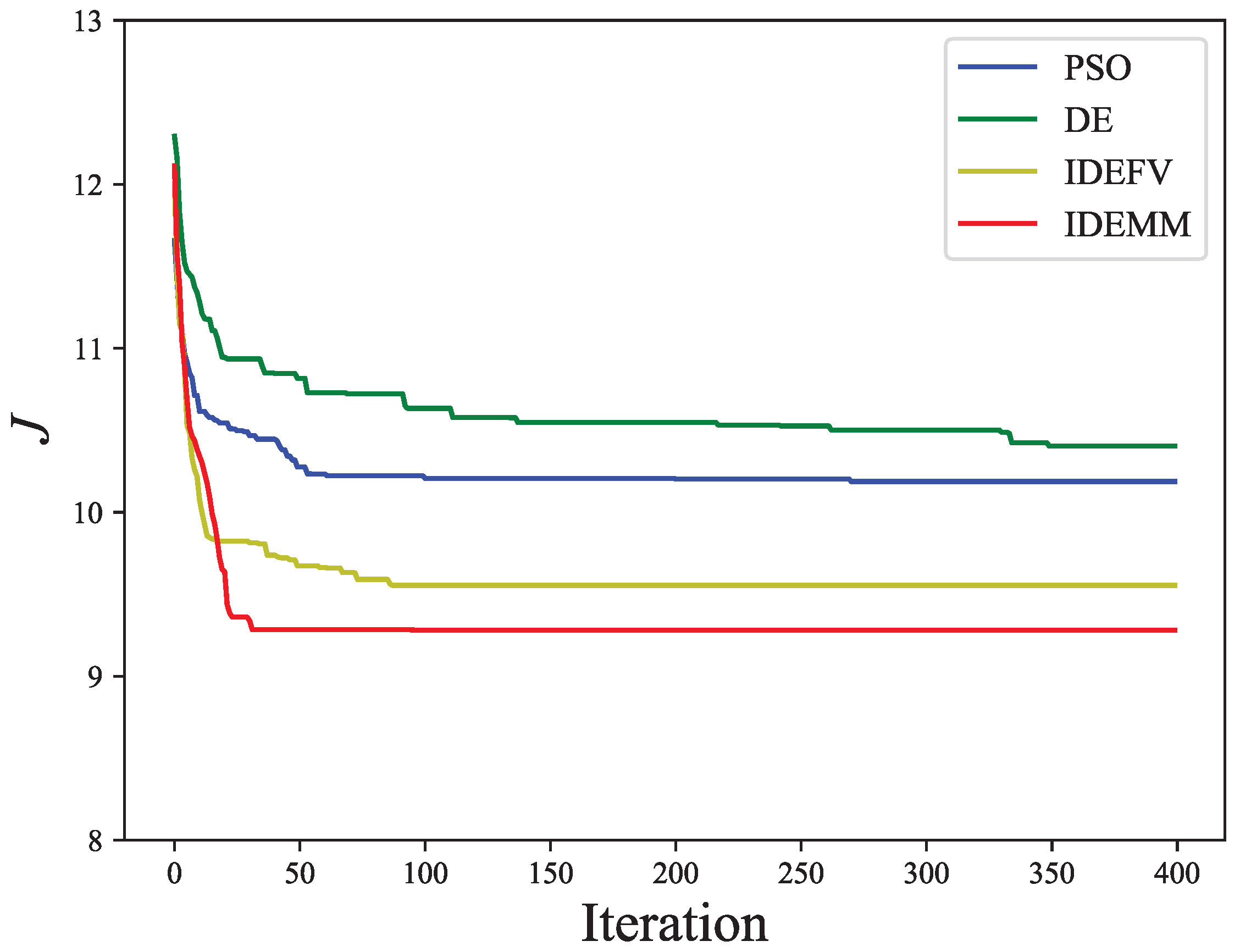
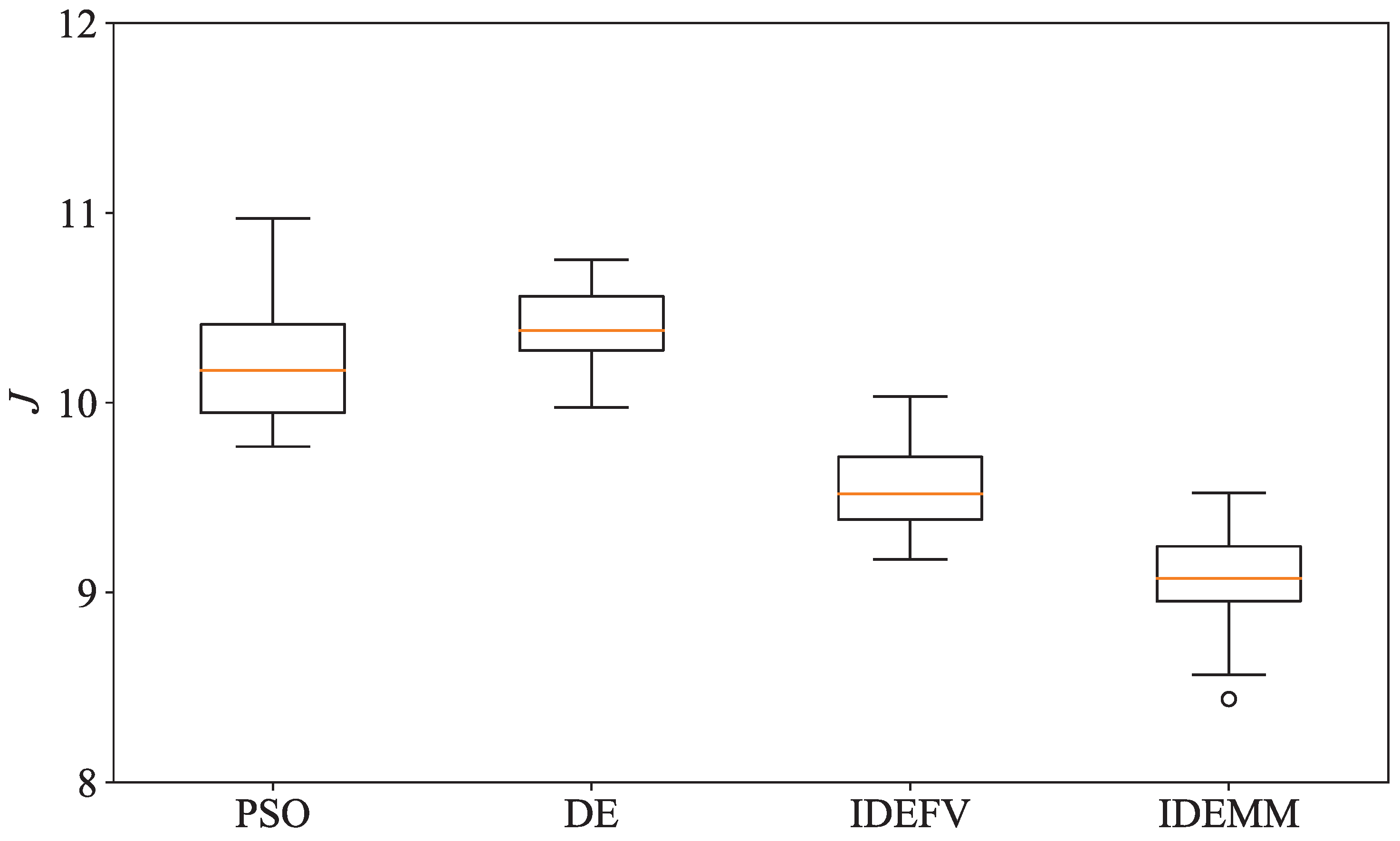
4.4. The Multi-UAV Cooperative Mission Planning
5. Conclusions
Author Contributions
Funding
Data Availability Statement
DURC Statement
Conflicts of Interest
References
- Jun, Z.; Jiahao, X. Cooperative task assignment of multi-UAV system. Chin. J. Aeronaut. 2020, 33, 2825–2827. [Google Scholar] [CrossRef]
- Fan, C.; Han, S.; Li, X.; Zhang, T.; Yuan, Y. A modified nature-inspired meta-heuristic methodology for heterogeneous unmanned aerial vehicle system task assignment problem. Soft Comput. 2021, 25, 14227–14243. [Google Scholar] [CrossRef]
- Wang, Z.; Zhang, J. A task allocation algorithm for a swarm of unmanned aerial vehicles based on bionic wolf pack method. Knowl. Based Syst. 2022, 250, 109072. [Google Scholar] [CrossRef]
- Chen, J.; Wu, Q.; Xu, Y.; Qi, N.; Guan, X.; Zhang, Y.; Xue, Z. Joint Task Assignment and Spectrum Allocation in Heterogeneous UAV Communication Networks: A Coalition Formation Game-Theoretic Approach. IEEE Trans. Wirel. Commun. 2020, 20, 440–452. [Google Scholar] [CrossRef]
- Schwarzrock, J.; Zacarias, I.; Bazzan, A.; Fernandes, R.; Moreira, L.; Pignaton de Freitas, E. Solving task allocation problem in multi Unmanned Aerial Vehicles systems using Swarm intelligence. Eng. Appl. Artif. Intell. 2018, 72, 10–20. [Google Scholar] [CrossRef]
- Li, J.; Yang, X.; Yang, Y.; Liu, X. Cooperative mapping task assignment of heterogeneous multi-UAV using an improved genetic algorithm. Knowl. Based Syst. 2024, 296, 111830. [Google Scholar] [CrossRef]
- Wu, Y. Task scheduling of the collaborative aerial–ground system for the search and capture of multiple targets. Knowl. Based Syst. 2022, 250, 109031. [Google Scholar] [CrossRef]
- Gao, X.; Wang, L.; Yu, X.; Su, X.c.; Ding, Y.; Lu, C.; Peng, H.; Wang, X. Conditional probability based multi-objective cooperative task assignment for heterogeneous UAVs. Eng. Appl. Artif. Intell. 2023, 123, 106404. [Google Scholar] [CrossRef]
- Chen, Y.; Yang, D.; Yu, J. Multi-UAV Task Assignment With Parameter and Time-Sensitive Uncertainties Using Modified Two-Part Wolf Pack Search Algorithm. IEEE Trans. Aerosp. Electron. Syst. 2018, 54, 2853–2872. [Google Scholar] [CrossRef]
- Jiang, S.; Yuan, X. Application of improved PSO algorithm in multi UAV cooperative task allocation. Appl. Res. Comput. 2019, 36, 3344–3347+3360. [Google Scholar]
- Wu, X.; Yin, Y.; Xu, L.; Wu, X.; Meng, F.; Zhen, R. MULTI-UAV Task Allocation Based on Improved Genetic Algorithm. IEEE Access 2021, 9, 100369–100379. [Google Scholar] [CrossRef]
- Yu, X.; Gao, X.; Wang, L.; Wang, X.; Ding, Y.; Lu, C.; Zhang, S. Cooperative Multi-UAV Task Assignment in Cross-Regional Joint Operations Considering Ammunition Inventory. Drones 2022, 6, 77. [Google Scholar] [CrossRef]
- Zhu, J.; Wu, G.; Li, Z. A Novel Simulated Annealing Based Strategy for Balanced UAV Task Assignment and Path Planning. Sensors 2020, 20, 4769. [Google Scholar] [CrossRef] [PubMed]
- Luo, R.; Zheng, H.; Guo, J. Solving the Multi-Functional Heterogeneous UAV Cooperative Mission Planning Problem Using Multi-Swarm Fruit Fly Optimization Algorithm. Sensors 2020, 20, 5026. [Google Scholar] [CrossRef] [PubMed]
- Yu, X.; Li, X.; Wang, L.; Jin, J.; Zhang, G.; Su, X.; Tao, L.; Lu, C.; Wang, X. Carrier platform-enhanced multiple-UAV cooperative task assignment with dual heterogeneities. Artif. Intell. Rev. 2025, 58, 248. [Google Scholar]
- Jin, J.; Zhang, G.; Li, X.; Su, X.; Lu, C.; Cheng, Y.; Ding, Y.; Wang, L.; Wang, X. Cross-platform mission planning for UAVs under carrier delivery mode. Def. Technol. 2025, in press. [Google Scholar] [CrossRef]
- Ma, H.; Zhu, Y.M.; Hu, X. Cooperative task planning for ship and UAVs based on particle swarm optimization algorithm. Syst. Eng. Electron. 2016, 38, 1583–1588. [Google Scholar]
- Jiang, J.; Dai, Y.; Yang, F.; Ma, Z. A multi-visit flexible-docking vehicle routing problem with drones for simultaneous pickup and delivery services. Eur. J. Oper. Res. 2023, 312, 125–137. [Google Scholar] [CrossRef]
- Salama, M.; Srinivas, S. Collaborative truck multi-drone routing and scheduling problem: Package delivery with flexible launch and recovery sites. Transp. Res. Part E Logist. Transp. Rev. 2022, 164, 102788. [Google Scholar] [CrossRef]
- Roytvand Ghiasvand, M.; Rahmani, D.; Moshref-Javadi, M. Data-driven robust optimization for a multi-trip truck-drone routing problem. Expert Syst. Appl. 2024, 241, 122485. [Google Scholar] [CrossRef]
- Yan, R.; Zhu, X.; Zhu, X.; Peng, R. Optimal Routes and Aborting Strategies of Trucks and Drones under Random attacks. Reliab. Eng. Syst. Saf. 2022, 222, 108457. [Google Scholar] [CrossRef]
- Murray, C.; Raj, R. The multiple flying sidekicks traveling salesman problem: Parcel delivery with multiple drones. Transp. Res. Part C Emerg. Technol. 2020, 110, 368–398. [Google Scholar] [CrossRef]
- Wang, X.; Li, B.; Su, X.C.; Peng, H.; Wang, L.; Lu, C.; Wang, C. Autonomous dispatch trajectory planning on flight deck: A search-resampling-optimization framework. Eng. Appl. Artif. Intell. 2023, 119, 105792. [Google Scholar] [CrossRef]
- Wang, X.; Deng, Z.; Peng, H.; Wang, L.; Wang, Y.; Tao, L.; Lu, C.; Peng, Z. Autonomous docking trajectory optimization for unmanned surface vehicle: A hierarchical method. Ocean Eng. 2023, 279, 114156. [Google Scholar] [CrossRef]
- Li, X.; Wang, L.; Wang, H.; Tao, L.; Wang, X. A Warm-started Trajectory Planner for Fixed-wing Unmanned Aerial Vehicle Formation. Appl. Math. Model. 2023, 122, 200–219. [Google Scholar] [CrossRef]
- Trovato, K.; Dorst, L. Differential A*. IEEE Trans. Knowl. Data Eng. 2002, 14, 1218–1229. [Google Scholar] [CrossRef]
- Xie, L.; Xue, S.; Zhang, J.; Zhang, M.; Tian, W.; Haugen, S. A path planning approach based on multi-direction A* algorithm for ships navigating within wind farm waters. Ocean Eng. 2019, 184, 311–322. [Google Scholar] [CrossRef]
- Wu, X.; Xu, L.; Zhen, R.; Wu, X. Bi-Directional Adaptive A* Algorithm Toward Optimal Path Planning for Large-Scale UAV Under Multi-Constraints. IEEE Access 2020, 8, 85431–85440. [Google Scholar] [CrossRef]
- Song, R.; Liu, Y.; Bucknall, R. Smoothed A* algorithm for practical unmanned surface vehicle path planning. Appl. Ocean. Res. 2019, 83, 9–20. [Google Scholar] [CrossRef]
- Hawa, M. Light-Assisted Path Planning. Eng. Appl. Artif. Intell. 2013, 26, 888–898. [Google Scholar] [CrossRef]
- Wang, X.; Wang, H.; Zhang, H.; Wang, M.; Wang, L.; Cui, K.; Lu, C.; Ding, Y. A mini review on UAV mission planning. J. Ind. Manag. Optim. 2022, 19, 3362–3382. [Google Scholar] [CrossRef]
- Liu, Y.; Qi, N.; Yao, W.; Zhao, J.; Xu, S. Cooperative Path Planning for Aerial Recovery of a UAV Swarm Using Genetic Algorithm and Homotopic Approach. Appl. Sci. 2020, 10, 4154. [Google Scholar] [CrossRef]
- Zhao, B.; Huo, M.; Yu, Z.; Qi, N.; Wang, J. Model-Reference Reinforcement Learning for Safe Aerial Recovery of Unmanned Aerial Vehicles. Aerospace 2024, 11, 27. [Google Scholar] [CrossRef]
- Xing, Z.; Zhang, L.; Ai, J. Research of key technologies for multi-rotor UAV automatic aerial recovery system. Electron. Lett. 2022, 58, 277–279. [Google Scholar] [CrossRef]
- Zhang, G.; Wang, L.; Deng, Z.; Liu, X.; Su, X.; Li, H.; Lu, C.; Liu, K.; Wang, X. Landing scheduling for carrier aircraft fleet considering bolting probability and aerial refueling. Def. Technol. 2025, in press. [Google Scholar] [CrossRef]
- Wang, G.G.; Chu, H.; Mirjalili, S. Three-dimensional path planning for UCAV using an improved bat algorithm. Aerosp. Sci. Technol. 2016, 49, 231–238. [Google Scholar] [CrossRef]
- Cheng, Z.; Zhao, L.; Shi, Z. Decentralized Multi-UAV Path Planning Based on Two-Layer Coordinative Framework for Formation Rendezvous. IEEE Access 2022, 10, 45695–45708. [Google Scholar] [CrossRef]
- Zhang, Z.; Liu, H.; Wu, G. A Dynamic Task Scheduling Method for Multiple UAVs Based on Contract Net Protocol. Sensors 2022, 22, 4486. [Google Scholar] [CrossRef] [PubMed]
- Wang, G.; Lv, X.; Yan, X. A Two-Stage Distributed Task Assignment Algorithm Based on Contract Net Protocol for Multi-UAV Cooperative Reconnaissance Task Reassignment in Dynamic Environments. Sensors 2023, 23, 7980. [Google Scholar] [CrossRef] [PubMed]
- Lee, D.H.; Zaheer, S.A.; Kim, J.H. A Resource-Oriented, Decentralized Auction Algorithm for Multirobot Task Allocation. IEEE Trans. Autom. Sci. Eng. 2015, 12, 1469–1481. [Google Scholar] [CrossRef]
- Ming, Z.; Lingling, Z.; Xiaohong, S.; Peijun, M.; Yanhang, Z. Improved discrete mapping differential evolution for multi-unmanned aerial vehicles cooperative multi-targets assignment under unified model. Int. J. Mach. Learn. Cybern. 2015, 8, 765–780. [Google Scholar] [CrossRef]
- Su, J.l.; Wang, H. An improved adaptive differential evolution algorithm for single unmanned aerial vehicle multitasking. Def. Technol. 2021, 17, 1967–1975. [Google Scholar] [CrossRef]
- Kuffner, J.; LaValle, S. RRT-connect: An efficient approach to single-query path planning. IEEE Int. Conf. Robot. Autom. Symp. Proc. 2000, 2, 995–1001. [Google Scholar]
- Salgotra, R.; Gandomi, A. A novel multi-hybrid differential evolution algorithm for optimization of frame structures. Sci. Rep. 2024, 14, 4877. [Google Scholar] [CrossRef]
- Manoranjani, M.; Sukumaran, S. Performance of ML-Based Unsupervised Clustering Algorithms for WSN Node Clustering. Int. J. Res. Appl. Sci. Eng. Technol. 2024, 12, 153–158. [Google Scholar] [CrossRef]
- Xu, R. Path planning of mobile robot based on multi-sensor information fusion. J. Wirel. Commun. Netw. 2019, 44, 44. [Google Scholar] [CrossRef]
- Resilient multi-objective mission planning for UAV formation: A unified framework integrating task pre- and re-assignment. Def. Technol. 2025, 45, 203–226. [CrossRef]
- Gao, X.; Wang, L.; Su, X.; Lu, C.; Ding, Y.; Wang, C.; Peng, H.; Wang, X. A Unified Multi-Objective Optimization Framework for UAV Cooperative Task Assignment and Re-Assignment. Mathematics 2022, 10, 4241. [Google Scholar] [CrossRef]

| Symbol | Meaning | Value |
|---|---|---|
| N | The number of DPs | 8 |
| The maximum ammunition load of UAV | 3 | |
| The ammunition number needed for the attack task | 1 | |
| The maximum flight time of UAV (h) | 10 | |
| The detection radius of the radar (km) | 80 | |
| The flight speed of UAV (km/h) | 100 | |
| The time interval between tasks (h) | 0.1 | |
| The search radius of the DP (km) | 50 |
| Parameter | Meaning | Value |
|---|---|---|
| The population size | 50 | |
| The maximum iteration | 400 | |
| The variation rate | 0.1 | |
| The weight of actual radar threat | ||
| The weight of predicted radar threat | 10 |
| Parameter | Meaning | Value |
|---|---|---|
| The population size | 50 | |
| The maximum iterations | 400 | |
| The scaling factor for the number of dropped UAVs | 3 | |
| The penalty factor of remaining flight time | 0.8 | |
| The penalty factor of remaining ammunition | 0.2 |
| Number | Location (km) | Number | Location (km) |
|---|---|---|---|
| (772,729) | (467,891) | ||
| (890,195) | (154,290) | ||
| (847,640) | (283,811) | ||
| (189,639) | (491,155) |
| AC Path Length (km) | Deployed UAV Number | Execution Time (h) | |
|---|---|---|---|
| N = 6 | 2966.94 | 54 | 7.9 |
| N = 8 | 3128.13 | 51 | 8.3 |
| N = 10 | 3208.97 | 49 | 9.6 |
| RRT | Proposed Algorithm | |||
|---|---|---|---|---|
| Runtime (s) | Path Length (km) | Runtime (s) | Path Length (km) | |
| 19.94 | 1094.76 | 5.18 | 950.31 | |
| 10.09 | 764.93 | 1.58 | 684.74 | |
| 16.61 | 1147.26 | 3.95 | 941.68 | |
| 3105.81 | 33.10 | ||
| 3110.54 | 91.43 | ||
| 3162.46 | 250.63 | ||
| 3341.18 | 907.58 |
| UAV | Task List | Execution Time (h) |
|---|---|---|
| 7.9 | ||
| 6.5 | ||
| 7.6 | ||
| 7.4 | ||
| 7.1 | ||
| 7.4 |
| PSO | DE | IDEFV | IDEMM | |
|---|---|---|---|---|
| Std | 0.35 | 0.24 | 0.25 | 0.23 |
| Mean | 10.22 | 10.39 | 9.58 | 9.05 |
Disclaimer/Publisher’s Note: The statements, opinions and data contained in all publications are solely those of the individual author(s) and contributor(s) and not of MDPI and/or the editor(s). MDPI and/or the editor(s) disclaim responsibility for any injury to people or property resulting from any ideas, methods, instructions or products referred to in the content. |
© 2025 by the authors. Licensee MDPI, Basel, Switzerland. This article is an open access article distributed under the terms and conditions of the Creative Commons Attribution (CC BY) license (https://creativecommons.org/licenses/by/4.0/).
Share and Cite
Zhang, H.; Li, B.; Wang, L.; Cheng, Y.; Ding, Y.; Lu, C.; Peng, H.; Wang, X. Mission Planning for UAV Swarm with Aircraft Carrier Delivery: A Decoupled Framework. Aerospace 2025, 12, 691. https://doi.org/10.3390/aerospace12080691
Zhang H, Li B, Wang L, Cheng Y, Ding Y, Lu C, Peng H, Wang X. Mission Planning for UAV Swarm with Aircraft Carrier Delivery: A Decoupled Framework. Aerospace. 2025; 12(8):691. https://doi.org/10.3390/aerospace12080691
Chicago/Turabian StyleZhang, Hongyun, Bin Li, Lei Wang, Yujie Cheng, Yu Ding, Chen Lu, Haijun Peng, and Xinwei Wang. 2025. "Mission Planning for UAV Swarm with Aircraft Carrier Delivery: A Decoupled Framework" Aerospace 12, no. 8: 691. https://doi.org/10.3390/aerospace12080691
APA StyleZhang, H., Li, B., Wang, L., Cheng, Y., Ding, Y., Lu, C., Peng, H., & Wang, X. (2025). Mission Planning for UAV Swarm with Aircraft Carrier Delivery: A Decoupled Framework. Aerospace, 12(8), 691. https://doi.org/10.3390/aerospace12080691