
Graph Neural Network-Enhanced Multi-Agent Reinforcement Learning for Intelligent UAV Confrontation


Abstract
1. Introduction
2. Mathematical Statements
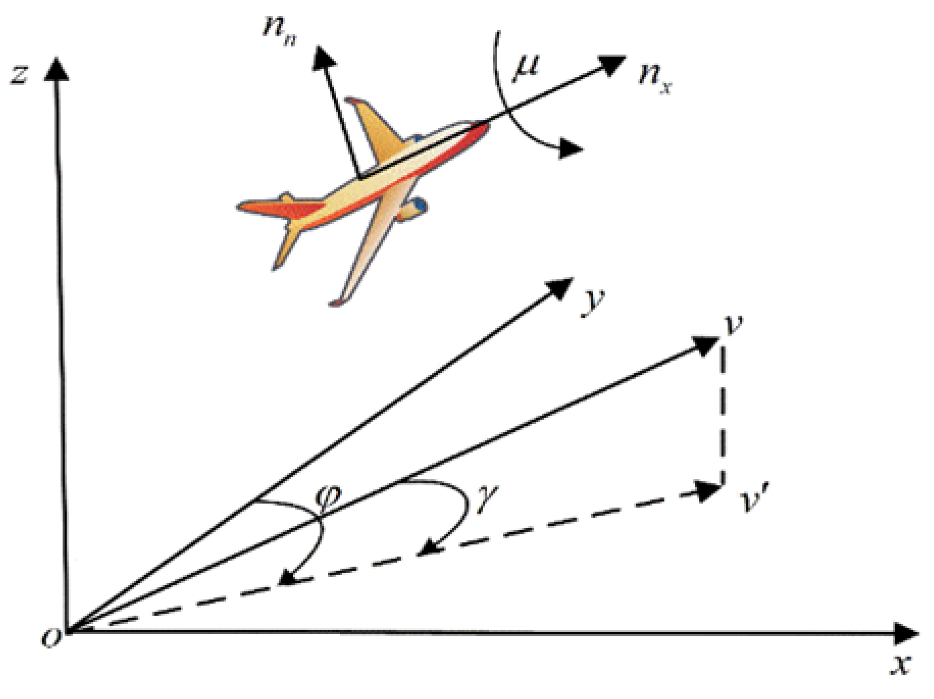
2.1. UAV Maneuver Model
2.2. Markov Decision Process for the UAV Game Confrontation Policy
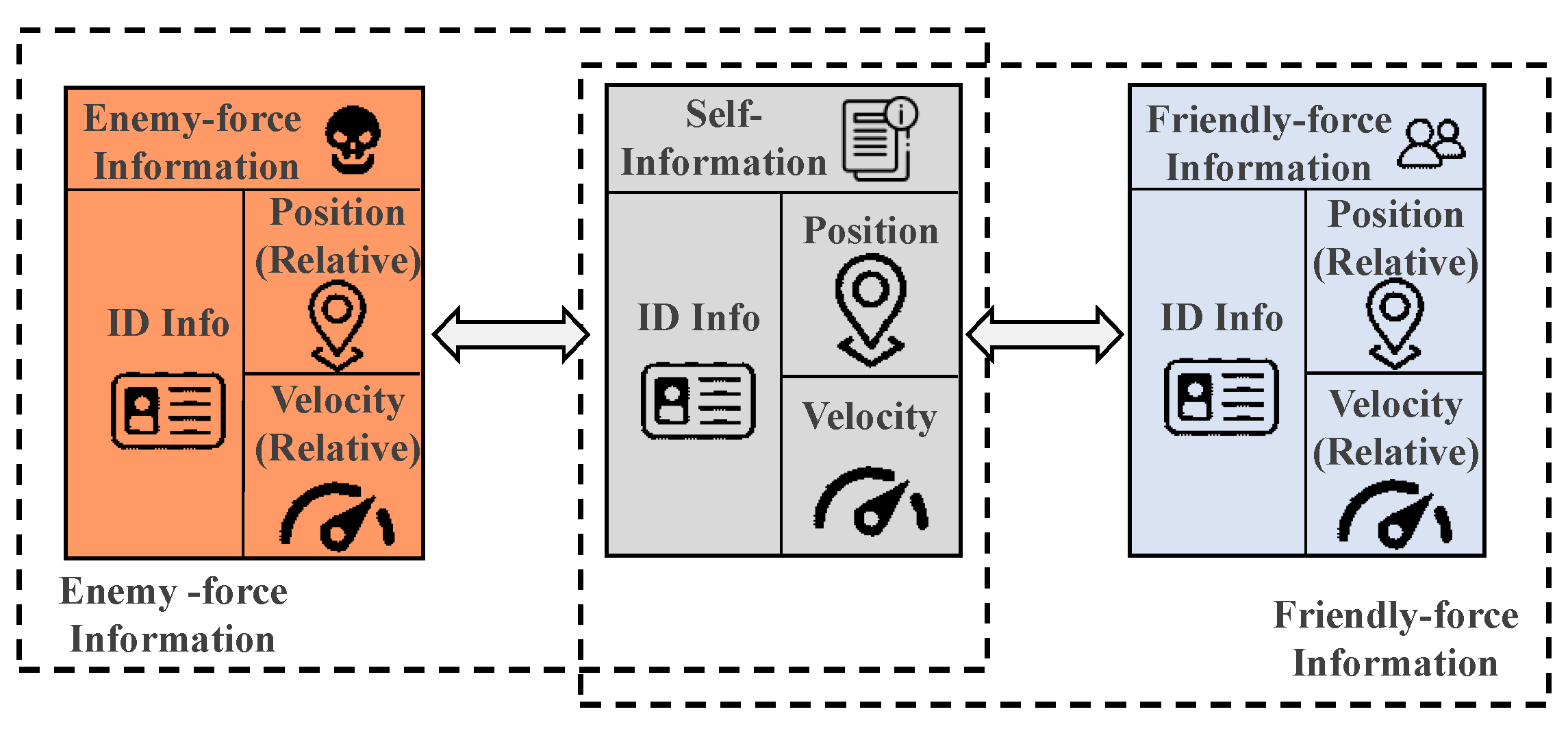
2.2.1. State Space
2.2.2. Action Space
2.2.3. Reward Function
3. Methodology
3.1. Intelligent Decision-Making Algorithm Based on GCN
3.2. Multi-Agent State Extraction Based on GCN
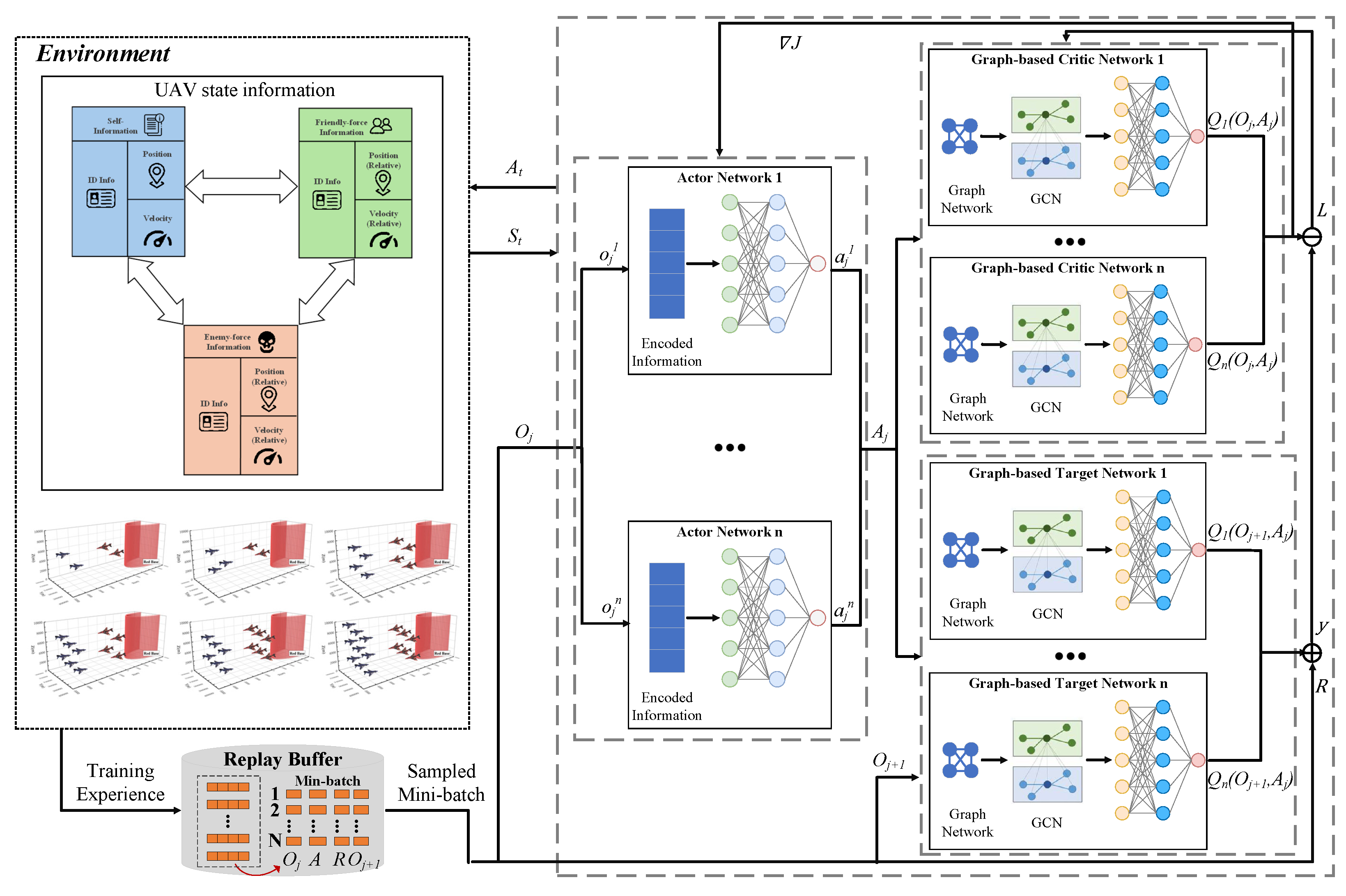
3.3. Training Process of Intelligent Decision-Making Algorithm Based on GCN
| Algorithm 1 G-MADDPG Algorithm |
| Input: Environment model , Number of training steps l, Number of episodes N, Discount factor , Experience pool size M, Sample size m, Target Network Update , Exploration-exploitation strategy Output: Optimal policy
|
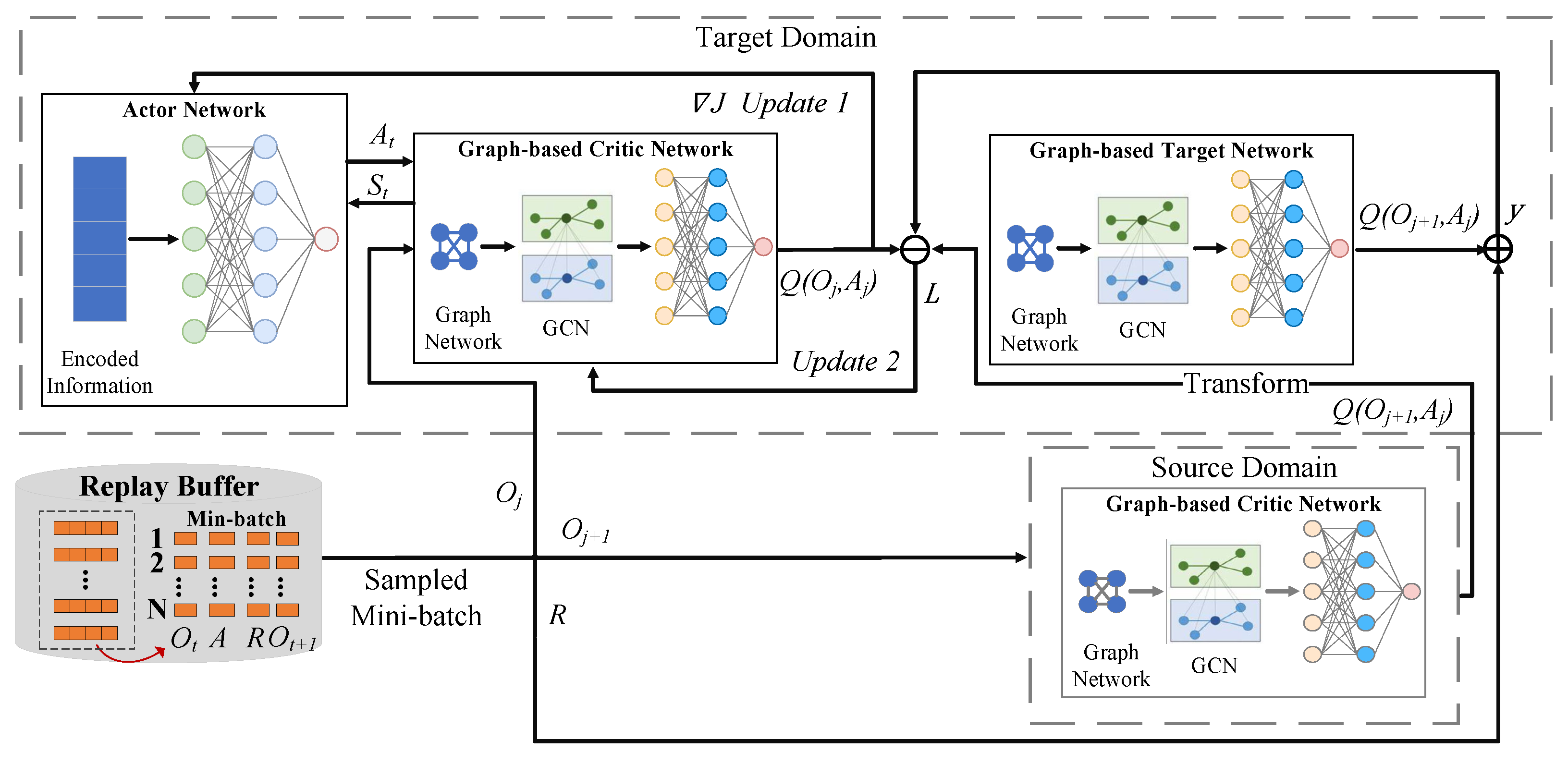
3.4. MARL Based on Transfer Learning
4. Simulation Verification
4.1. Simulation Settings
4.1.1. Parameter Settings
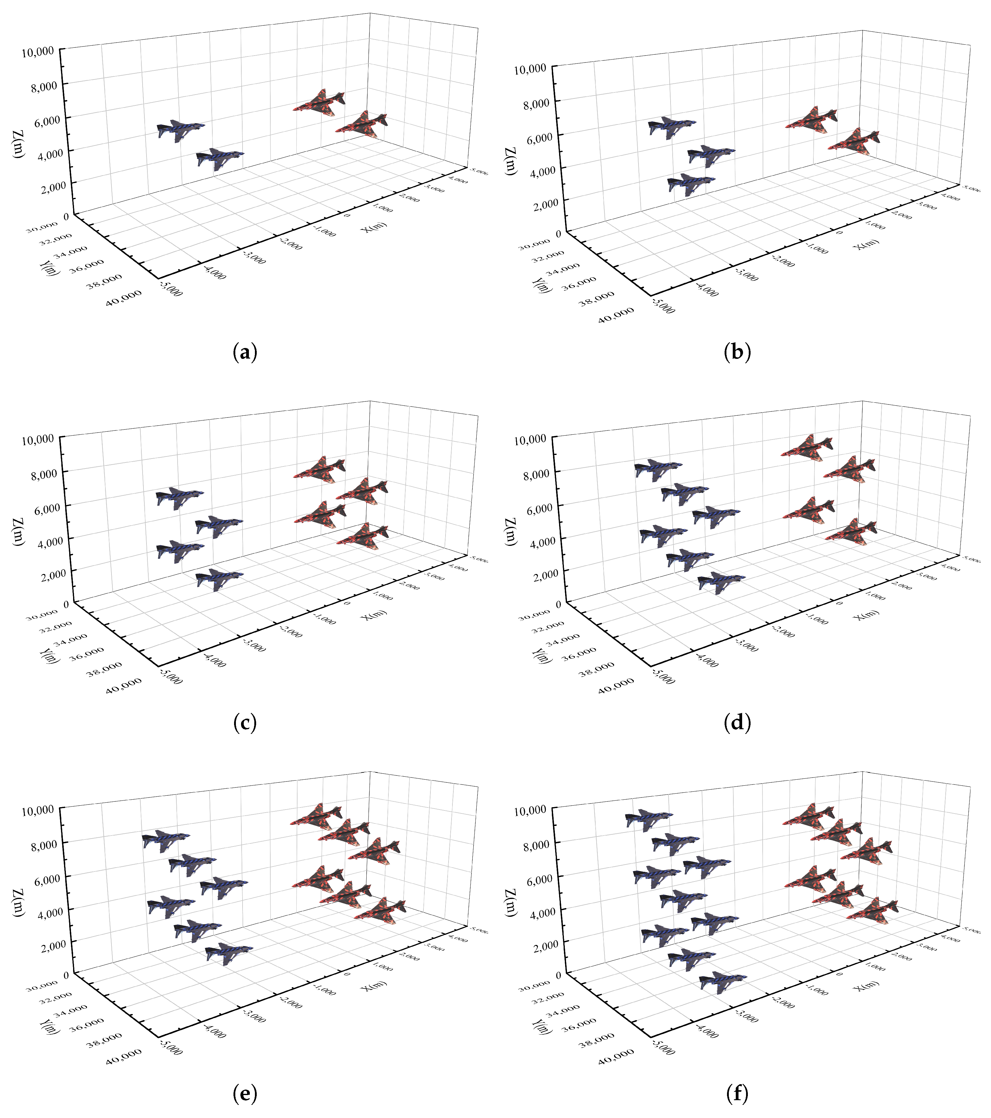
4.1.2. Scenarios Settings
4.2. Experimental Results
5. Conclusions
Author Contributions
Funding
Data Availability Statement
Conflicts of Interest
References
- Elmeseiry, N.; Alshaer, N.; Ismail, T. A detailed survey and future directions of unmanned aerial vehicles (uavs) with potential applications. Aerospace 2021, 8, 363. [Google Scholar] [CrossRef]
- Chen, Y.; Zhang, J.; Li, Z.; Zhang, H.; Chen, J.; Yang, W.; Yu, T.; Liu, W.; Li, Y. Manufacturing technology of lightweight fiber-reinforced composite structures in aerospace: Current situation and toward intellectualization. Aerospace 2023, 10, 206. [Google Scholar] [CrossRef]
- Sar, A.; Choudhury, T.; Singh, R.K.; Kumar, A.; Mahdi, H.F.; Vishnoi, A. Disruptive Technologies in Cyber-Physical Systems in War. In Cyber-Physical Systems for Innovating and Transforming Society 5.0; Scrivener Publishing LLC: Beverly, MA, USA, 2025; pp. 233–250. [Google Scholar]
- Navickiene, O.; Bekesiene, S.; Vasiliauskas, A.V. Optimizing Unmanned Combat Air Systems Autonomy, Survivability, and Combat Effectiveness: A Fuzzy DEMATEL Assessment of Critical Technological and Strategic Drivers. In Proceedings of the 2025 International Conference on Military Technologies (ICMT), Brno, Czech Republic, 27–30 May 2025; pp. 1–8. [Google Scholar]
- Insaurralde, C.C.; Blasch, E. Ontological Airspace-Situation Awareness for Decision System Support. Aerospace 2024, 11, 942. [Google Scholar] [CrossRef]
- Sandino Mora, J.D. Autonomous Decision-Making for UAVs Operating Under Environmental and Object Detection Uncertainty. Ph.D. Thesis, Queensland University of Technology, Brisbane, Australia, 2022. [Google Scholar]
- Ni, J.; Tang, G.; Mo, Z.; Cao, W.; Yang, S.X. An improved potential game theory based method for multi-UAV cooperative search. IEEE Access 2020, 8, 47787–47796. [Google Scholar] [CrossRef]
- Wang, L.; Lu, D.; Zhang, Y.; Wang, X. A complex network theory-based modeling framework for unmanned aerial vehicle swarms. Sensors 2018, 18, 3434. [Google Scholar] [CrossRef] [PubMed]
- Sarkar, N.I.; Gul, S. Artificial intelligence-based autonomous UAV networks: A survey. Drones 2023, 7, 322. [Google Scholar] [CrossRef]
- Mkiramweni, M.E.; Yang, C.; Li, J.; Zhang, W. A survey of game theory in unmanned aerial vehicles communications. IEEE Commun. Surv. Tutor. 2019, 21, 3386–3416. [Google Scholar] [CrossRef]
- Park, H.; Lee, B.Y.; Tahk, M.J.; Yoo, D.W. Differential game based air combat maneuver generation using scoring function matrix. Int. J. Aeronaut. Space Sci. 2016, 17, 204–213. [Google Scholar] [CrossRef]
- Zheng, H.; Deng, Y.; Hu, Y. Fuzzy evidential influence diagram and its evaluation algorithm. Knowl.-Based Syst. 2017, 131, 28–45. [Google Scholar] [CrossRef]
- Gao, Y.; Zhang, L.; Wang, C.; Zheng, X.; Wang, Q. An evolutionary game-theoretic approach to unmanned aerial vehicle network target assignment in three-dimensional scenarios. Mathematics 2023, 11, 4196. [Google Scholar] [CrossRef]
- Virtanen, K.; Raivio, T.; Hamalainen, R.P. Modeling pilot’s sequential maneuvering decisions by a multistage influence diagram. J. Guid. Control. Dyn. 2004, 27, 665–677. [Google Scholar] [CrossRef]
- Jiang, S.; Xie, W.; Zhang, L.; Zhang, G.; Liang, X.; Zheng, Y. Current status and development trends of research on autonomous decision-making methods for unmanned swarms. In Proceedings of the International Conference on Optics, Electronics, and Communication Engineering (OECE 2024), Wuhan, China, 26–28 July 2024; SPIE: Bellingham, WA, USA, 2024; Volume 13395, pp. 132–138. [Google Scholar]
- Canese, L.; Cardarilli, G.C.; Di Nunzio, L.; Fazzolari, R.; Giardino, D.; Re, M.; Spanò, S. Multi-agent reinforcement learning: A review of challenges and applications. Appl. Sci. 2021, 11, 4948. [Google Scholar] [CrossRef]
- Zhang, K.; Yang, Z.; Başar, T. Multi-agent reinforcement learning: A selective overview of theories and algorithms. In Handbook of Reinforcement Learning and Control; Springer: Cham, Switzerland, 2021; pp. 321–384. [Google Scholar]
- Hernandez-Leal, P.; Kartal, B.; Taylor, M.E. Is multiagent deep reinforcement learning the answer or the question? A brief survey. Learning 2018, 21, 22. [Google Scholar]
- Do, Q.T.; Hua, T.D.; Tran, A.T.; Won, D.; Woraphonbenjakul, G.; Noh, W.; Cho, S. Multi-UAV aided energy-aware transmissions in mmWave communication network: Action-branching QMIX network. J. Netw. Comput. Appl. 2024, 230, 103948. [Google Scholar] [CrossRef]
- Pan, Y.; Wang, X.; Xu, Z.; Cheng, N.; Xu, W.; Zhang, J.J. GNN-Empowered Effective Partial Observation MARL Method for AoI Management in Multi-UAV Network. IEEE Internet Things J. 2024, 11, 34541–34553. [Google Scholar] [CrossRef]
- Han, J.; Yan, Y.; Zhang, B. Towards Efficient Multi-UAV Air Combat: An Intention Inference and Sparse Transmission Based Multi-Agent Reinforcement Learning Algorithm. IEEE Trans. Artif. Intell. 2025. [Google Scholar] [CrossRef]
- Li, Y.; Dong, W.; Zhang, P.; Zhai, H.; Li, G. Hierarchical Reinforcement Learning with Automatic Curriculum Generation for Unmanned Combat Aerial Vehicle Tactical Decision-Making in Autonomous Air Combat. Drones 2025, 9, 384. [Google Scholar] [CrossRef]
- Yoon, N.; Lee, D.; Kim, K.; Yoo, T.; Joo, H.; Kim, H. STEAM: Spatial Trajectory Enhanced Attention Mechanism for Abnormal UAV Trajectory Detection. Appl. Sci. 2024, 14, 248. [Google Scholar] [CrossRef]
- Wang, X.; Wang, Y.; Su, X.; Wang, L.; Lu, C.; Peng, H.; Liu, J. Deep reinforcement learning-based air combat maneuver decision-making: Literature review, implementation tutorial and future direction. Artif. Intell. Rev. 2024, 57, 1. [Google Scholar] [CrossRef]
- Skarka, W.; Ashfaq, R. Hybrid Machine Learning and Reinforcement Learning Framework for Adaptive UAV Obstacle Avoidance. Aerospace 2024, 11, 870. [Google Scholar] [CrossRef]
- Zhang, Z.; Huang, Y.; Huang, W.; Pan, W.; Liao, Y.; Zhou, S. An auto-upgradable end-to-end pre-authenticated secure communication protocol for UAV-aided perception intelligent system. IEEE Internet Things J. 2024, 11, 30187–30203. [Google Scholar] [CrossRef]
- Guo, Y.; Xue, W.; Ma, W.; Ju, Z.; Li, Y. Research on Methods for Presenting Battlefield Situation Hotspots. In Proceedings of the 2024 11th International Conference on Dependable Systems and Their Applications (DSA), Taicang, China, 2–3 November 2024; pp. 313–319. [Google Scholar]
- Rashid, T.; Samvelyan, M.; De Witt, C.S.; Farquhar, G.; Foerster, J.; Whiteson, S. Monotonic value function factorisation for deep multi-agent reinforcement learning. J. Mach. Learn. Res. 2020, 21, 1–51. [Google Scholar]
- Wang, Q.; Hao, Y.; Cao, J. ADRL: An attention-based deep reinforcement learning framework for knowledge graph reasoning. Knowl.-Based Syst. 2020, 197, 105910. [Google Scholar] [CrossRef]
- Akinwale, O.; Mojisola, D.; Adediran, P. Consensus issues in multi-agent-based distributed control with communication link impairments. Niger. J. Technol. Dev. 2024, 21, 85–93. [Google Scholar] [CrossRef]
- Liu, Y.; Wang, W.; Hu, Y.; Hao, J.; Chen, X.; Gao, Y. Multi-agent game abstraction via graph attention neural network. In Proceedings of the AAAI Conference on Artificial Intelligence, New York, NY, USA, 7–12 February 2020; Volume 34, pp. 7211–7218. [Google Scholar]
- Li, B.; Wang, J.; Song, C.; Yang, Z.; Wan, K.; Zhang, Q. Multi-UAV roundup strategy method based on deep reinforcement learning CEL-MADDPG algorithm. Expert Syst. Appl. 2024, 245, 123018. [Google Scholar] [CrossRef]
- Zhang, Y.; Wu, Z.; Ma, Y.; Sun, R.; Xu, Z. Research on autonomous formation of multi-UAV based on MADDPG algorithm. In Proceedings of the 2022 IEEE 17th International Conference on Control & Automation (ICCA), Naples, Italy, 27–30 June 2022; pp. 249–254. [Google Scholar]
- Li, B.; Liang, S.; Gan, Z.; Chen, D.; Gao, P. Research on multi-UAV task decision-making based on improved MADDPG algorithm and transfer learning. Int. J.-Bio-Inspired Comput. 2021, 18, 82–91. [Google Scholar] [CrossRef]
- Zhang, Y.; Mou, Z.; Gao, F.; Jiang, J.; Ding, R.; Han, Z. UAV-enabled secure communications by multi-agent deep reinforcement learning. IEEE Trans. Veh. Technol. 2020, 69, 11599–11611. [Google Scholar] [CrossRef]


| UAV Parameters | Value |
|---|---|
| Maximum speed | 250 m/s |
| Minimum speed | 10 m/s |
| Maximum detection range | 10,000 m |
| Maximum attack range | 3000 m |
| Maximum yaw angular acceleration | 20° |
| Maximum health | 1 |
| Loss rate of health | 0.2 |
| Parameter Category | Parameter | Value | Description |
|---|---|---|---|
| General RL Parameters | Optimizer | Adam | Optimizer for both actor and critic networks. |
| Actor learning rate | 0.01 | Learning rate for the actor network optimizer. | |
| Critic learning rate | 0.01 | Learning rate for the critic network optimizer. | |
| Discount factor | 0.99 | Reward discount factor. | |
| Experience pool size | 1,000,000 | Maximum number of experiences stored. | |
| Experience pool sample size | 1024 | Number of experiences sampled for each update. | |
| Target network update | 0.01 | Soft update parameter for the target critic network. | |
| Training schedule | Max training episodes | 5000 | Fixed termination condition for training. |
| Max steps per episode | 500 | Maximum simulation steps within one episode. | |
| Warm-up episodes | 100 | Episodes using random actions to populate the buffer before training starts. | |
| Exploration strategy | Noise type | Gaussian | Additive noise for action exploration. |
| Initial noise std. | 1.0 | Initial standard deviation of the Gaussian noise. | |
| Noise decay rate | 0.9995 | Multiplicative decay factor applied to after each episode. | |
| Minimum noise std. | 0.05 | Floor value for the noise standard deviation. | |
| Transfer learning | Transfer rate | 0.5 | Weighting factor for the source critic loss term in Equation (28). |
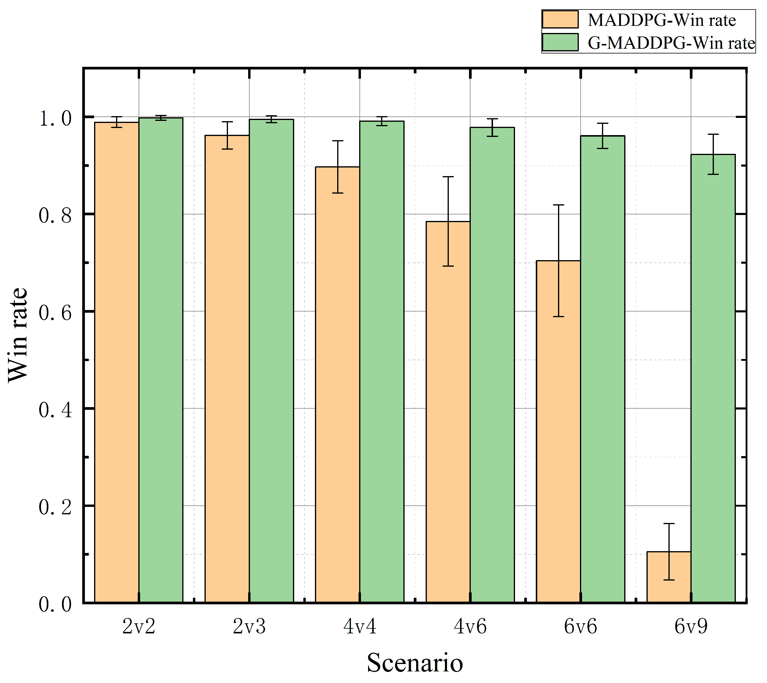
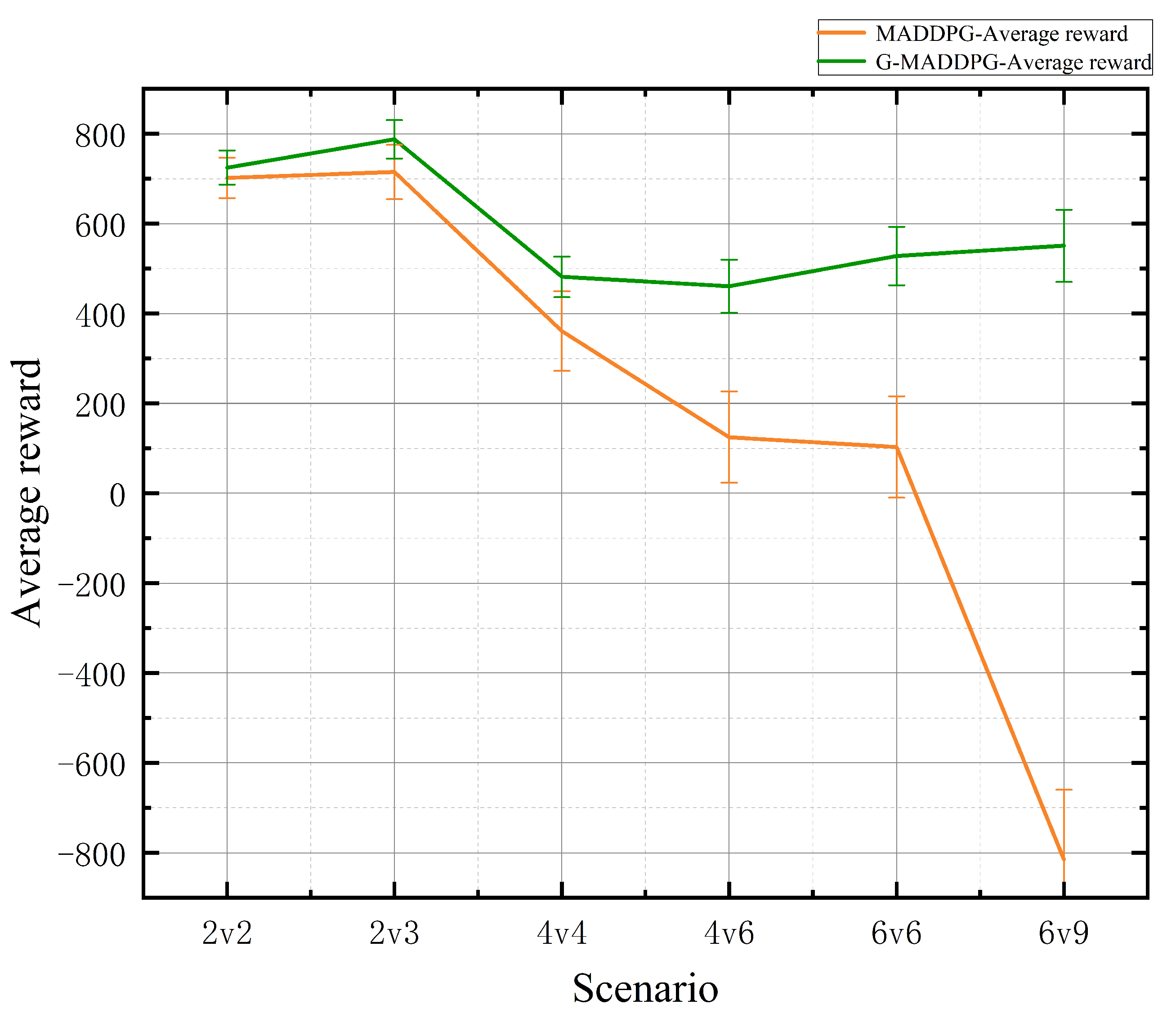
| Scenario | Method | Win Rate (Mean ± STD) | Average Reward (Mean ± STD) | p-Value (vs. MADDPG) |
|---|---|---|---|---|
| 2v2 | G-MADDPG | |||
| MADDPG | ||||
| 2v3 | G-MADDPG | |||
| MADDPG | ||||
| 4v4 | G-MADDPG | |||
| MADDPG | ||||
| 4v6 | G-MADDPG | |||
| MADDPG | ||||
| 6v6 | G-MADDPG | |||
| MADDPG | ||||
| 6v9 | G-MADDPG | |||
| MADDPG |
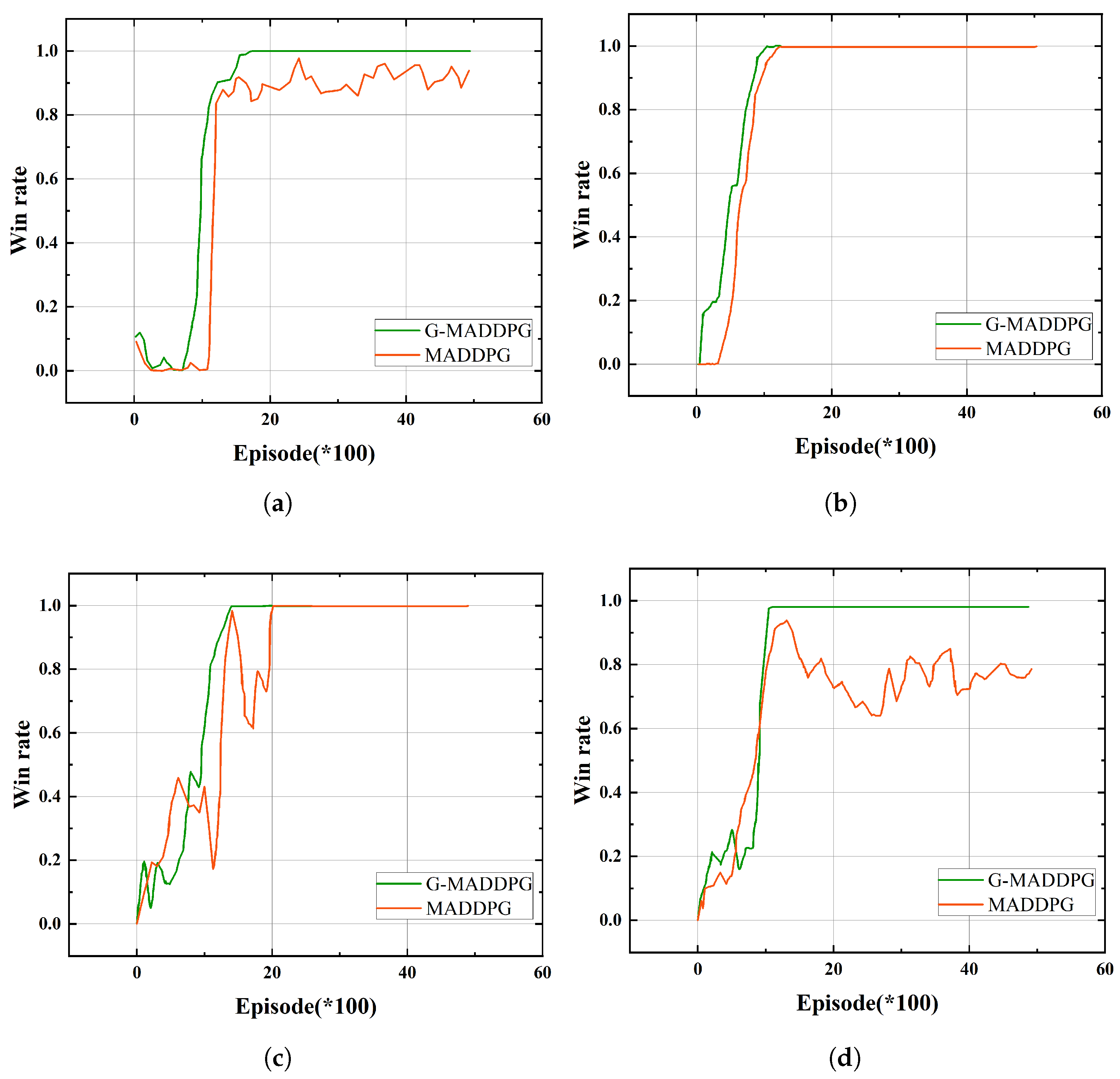
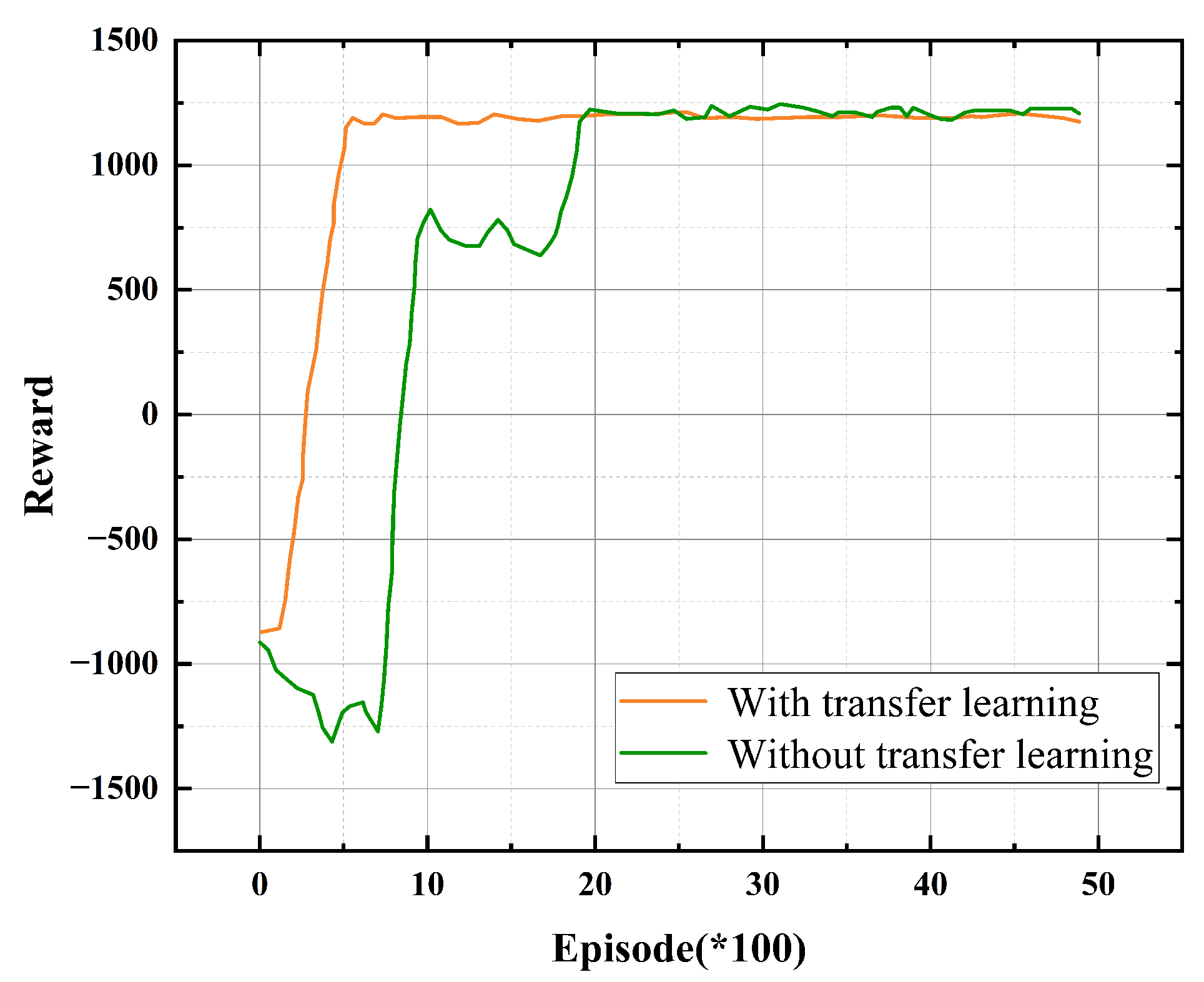
| Scenario | Iterations to Converge (TL) | Iterations to Converge (No TL) |
|---|---|---|
| 2v2 | 649 | 2034 |
| 2v3 | 673 | 2031 |
| 4v4 | 698 | 2489 |
Disclaimer/Publisher’s Note: The statements, opinions and data contained in all publications are solely those of the individual author(s) and contributor(s) and not of MDPI and/or the editor(s). MDPI and/or the editor(s) disclaim responsibility for any injury to people or property resulting from any ideas, methods, instructions or products referred to in the content. |
© 2025 by the authors. Licensee MDPI, Basel, Switzerland. This article is an open access article distributed under the terms and conditions of the Creative Commons Attribution (CC BY) license (https://creativecommons.org/licenses/by/4.0/).
Share and Cite
Hu, K.; Pan, H.; Han, C.; Sun, J.; An, D.; Li, S. Graph Neural Network-Enhanced Multi-Agent Reinforcement Learning for Intelligent UAV Confrontation. Aerospace 2025, 12, 687. https://doi.org/10.3390/aerospace12080687
Hu K, Pan H, Han C, Sun J, An D, Li S. Graph Neural Network-Enhanced Multi-Agent Reinforcement Learning for Intelligent UAV Confrontation. Aerospace. 2025; 12(8):687. https://doi.org/10.3390/aerospace12080687
Chicago/Turabian StyleHu, Kunhao, Hao Pan, Chunlei Han, Jianjun Sun, Dou An, and Shuanglin Li. 2025. "Graph Neural Network-Enhanced Multi-Agent Reinforcement Learning for Intelligent UAV Confrontation" Aerospace 12, no. 8: 687. https://doi.org/10.3390/aerospace12080687
APA StyleHu, K., Pan, H., Han, C., Sun, J., An, D., & Li, S. (2025). Graph Neural Network-Enhanced Multi-Agent Reinforcement Learning for Intelligent UAV Confrontation. Aerospace, 12(8), 687. https://doi.org/10.3390/aerospace12080687