Abstract
As accuracy of the reflector surface of a space parabolic deployable antenna is an important factor to determine its electrical characteristics (transmission gain and side lobes), mechanical characteristics of parabolic antennas under various internal pressures should be studied. The objective of this paper is to explore the force analysis of parabolic antennas by theoretical method and to estimate the effect of different air pressures on the surface precision of parabolic antennas via experiments in horizontal and vertical directions, and then a numerical analysis of the vibration characteristics of the parabolic antenna is proposed to explore the transient response of parabolic antennas. It is found that the ratio of tension reduces as depth of the parabolic membrane increases and can infinitely converge to 1/2. For precision analysis, it is concluded that precision of the parabolic membrane surface in a vertical state is higher than that in a horizontal state.
1. Introduction
Effective aperture and reflector precision of inflatable deployable parabolic membrane antennas can be considered as important factors to decide the performance of parabolic antennas [1]. Inflatable deployable antennas can be composed of an inflatable membrane reflector, supporting rings, and tension cables. The reflector of an inflatable parabolic antenna can be connected to supporting rings via tension cables. Each tension cable and edge cable is connected at the skirt corner to supporting rings, forming a complete inflatable parabolic antenna. Once the antenna is released into space, it can start to inflate. Three braces can be firstly inflated and deployed automatically (the braces are not included in the parabolic antenna in this paper), as the air can be imported into supporting rings, and deployment of supporting rings can tension cables so that tensile force can be imported into the parabolic membrane surface via skirts and edge cables. Then, the reflector starts to inflate and completely deploys to its design shape under internal pressure and supporting force from the supporting rings. Finally, the inflatable membrane antenna accesses the hardening stage. After the hardening stage, the inflatable deployable antenna can be transferred from a flexible membrane system to a flexible shell system; then the antenna can start to work after on track posture adjustment [2]. Inflatable deployable antennas have characteristics that have a low failure probability, high reliability and simple manufacturing process but low shape precision [3,4,5,6]. To design the inflatable deployable membrane antenna structures, stiffness, stress distribution, stress magnitudes and gravity effect should be explored [7]. As the deployment and deformation of inflatable deployable membrane antenna structures is a large deformation process, geometrical nonlinearity should be performed [8,9,10,11].
Some researchers have been focusing on the mechanical characteristics of inflatable deployable membrane antenna structures under various loading states. Li et al. [12] created a large-scale air inflated arch structure as a temporary pavilion by using both a dynamic deflation simulation and an experimental test. They concluded that the higher the initial internal pressure was, the longer the collapse duration was. Wang et al. [13] studied the interaction between the inner air and enveloping membrane of inflated membrane tubes under both axial compression and transverse bending. They found that the inflated tube with constant air mass had a larger critical wrinkling load and higher ultimate bearing capacity than those of the corresponding tube with a constant inner pressure, considering the effect of interaction between the inner air and enveloping membrane. Sun et al. [14] investigated the wind pressure acting on ridge–valley tensile membrane antenna structures through wind tunnel experiments; they thought that the terrain roughness of the ridge–valley tensile membrane antenna structures showed a mild influence on the mean wind pressure, whereas the eaves height exhibited minimal influence. Liu et al. [15] theoretically estimated the parameter sensitivity of an inflatable membrane antenna to accurately control its mechanical states. It can be observed that the influence of the variation in the factors, including the elastic modulus, pressure, Poisson’s ratio, and pre-stress on the mechanical states of the inflatable membrane antenna, could not be amplified. Samy et al. [16] explored the bagging effect and rupture failure of membrane antenna structures under persistent rainfall. It can be found that the crack on the inflatable fabric spread radially around, resulting in disproportionate destruction, while a major crack on the tension fabric reached the margin of the ponding area and ceased spreading. Liu et al. [17] developed the dynamic response of a typical four-point pretensioned saddle membrane structure under hail impact load by using numerical simulations and experimental studies. Wang et al. [18] proposed a numerical method based on the vector form intrinsic finite element (VFIFE) method for the mechanical analysis of non-prestressed cable-membrane structures, providing a reference for practical engineering problems with strong nonlinear characteristics. Zhong et al. [19] proposed an improved crease-free method for membrane structures by introducing arc-shaped slits, derived a quantitative relationship between the mechanical properties of the membrane structure and the dimensions of the slits and established an optimization design model for the slits to ensure the strength of the structure. Liu et al. [20] studied the random vibration and structural reliability of composite hyperbolic–parabolic membrane structures under wind load, providing important references for the design and analysis of membrane structures. Colin et al. [21] studied the buckling of a thin film deposited on an infinitely rigid substrate and its delamination over a finite length and analyzed the mechanical properties of the film. Li et al. [22] studied the stochastic dynamic response and reliability of a hyperbolic paraboloid membrane structure subjected to non-Gaussian wind load excitation.
Although numerous studies have been conducted on the structural mechanical properties of parabolic membrane antennas, this paper provides a more comprehensive analysis of their structural performance. In this paper, the analytical solutions of force analysis and deformation of the parabolic antenna under internal pressures are proposed in the Section 1. The Section 2 utilizes experiments to perform a precision analysis of the parabolic antenna in both horizontal and vertical states under different pressures. Finally, to explore the vibration characteristics of the membrane reflectors, the natural frequencies and mode shapes of the parabolic antenna are numerically simulated for the analysis of transient response in Section 3.
2. Analytical Solutions
2.1. Standard Equations
To design the inflatable parabolic reflectors, the mechanical characteristics of the parabolic antenna should be estimated. As the design of the membrane segments on the reflector are key technology, it is important to perform a force analysis of the parabolic antenna with a certain internal air pressure. In this section, the force expressions of the parabolic membrane surface in longitudinal and latitudinal directions can be obtained according to the membrane theory; then, force expressions of tensioning points on the skirt edges of the inflatable deployable membrane reflector can be deduced and parametric analysis can also be performed.
Figure 1 describes the prototype and geometrical data of 3 m parabolic membrane reflectors. Diameter of prototype antenna is 3000 mm, prototype antenna aperture is 3132.863 mm and depth of parabola is 170.292 mm, as shown in Figure 1. According to Figure 1b, the coordinates of focal point F of the parabola is (p/2, 0); the focal length AF is p/2. The distance between alignment L and the y-axis is p/2. Line MF is the focus radius. According to Figure 1c, the diameter DC of the prototype antenna is 3000 mm, the distance BF from the focal point to the prototype antenna aperture is 3132.863 mm. Depth AB of the parabola is 170.292 mm.
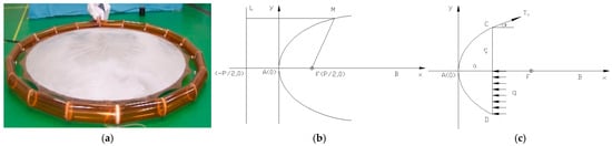
Figure 1.
Prototype and geometric data of 3 m inflatable deployable parabolic membrane reflectors. (a) Prototype; (b) Standard parabola curves; (c) Analytical model.
Therefore, the corresponding parabola equation is obtained in Equation (1):
where is the focal parameter, which represents the distance from the focus to the corresponding directrix in an ellipse. The corresponding polar coordinates can be obtained in Equation (2):
For parabolic surface membrane antenna structures, its equation can be obtained in Equation (3):
2.2. Surface Area and Volume Formula
The area of a curved surface can be given in Equation (4):
In the formula, A represents the area of a curved surface, where projective plane is a circular plane with a radius of . The corresponding polar coordinates can be transferred into Equation (5):
The volume formula of a rotating body can be obtained in Equation (6):
According to Equations (1) and (6), the volume formula of parabolic surface membrane antenna structures can be obtained in Equation (7):
According to Figure 1c, due to the symmetry of the reflector under internal air pressure, the schematic diagram of the membrane surface can be shown in Figure 1. q is the air pressure and T1 and T2 are, respectively, tension forces in the longitudinal and latitudinal direction. R1 and R2 are, respectively, corresponding principle curvature radii of membrane surface, is radius of curvature of margin of parabolic surface. is radius of projection plane of parabolic surface. is depth, F is focal point of parabolic surface.
2.3. Tension Forces in Longitudinal Direction
For the T1 tension force in longitudinal direction, the equilibrium equation in x-axis direction can be obtained in Equation (8):
Therefore, it can be written as Equation (9):
As the slope of parabola is known; therefore, the slope K can be obtained in Equation (10):
According to the definition of slope, Equation (11) can be given as follows:
Therefore, Equation (12) can be obtained:
As shown in Figure 1c, is the tension in longitudinal direction of the membrane surface. According to Equations (9)–(13), the tension force in longitudinal direction can be obtained into Equation (13):
According to Equation (13), at the top of the parabolic antenna, the can be simplified into Equation (14):
According to Equations (12) and (13), the tension on the membrane surface in x-axis and y-axis as shown in Figure 1c can be obtained in Equation (15):
2.4. Tension Forces in Latitudinal Direction
According to Equation (15), the tension force in longitudinal direction and its axis component of force in y-axis direction reduces with antenna aperture reduces along the x-axis whereas its axis component of force in x-axis direction is constant.
For the tension forces in the latitudinal direction, the equilibrium equation of infinitesimal of the parabolic membrane surface can be obtained in Equation (16):
where and are, respectively, the principal radius of curvature in the longitudinal and latitudinal direction. is normal pressure, = q.
According to the formula of slope in Equation (17) and parabolic Equation (1):
The curvature of paraboloid in the longitudinal direction can be obtained in Equation (18):
As shown in Figure 1c, and are the corresponding membrane curvature radius, and is the tension in the latitudinal direction of the membrane surface. Therefore, the radius of curvature in the longitudinal direction can be obtained in Equation (19):
The radius of curvature in the latitudinal direction can be obtained in Equation (20):
Taking Equations (13), (19) and (20) into Equation (16), the tension forces in the latitudinal direction can be obtained in Equation (21).
At the top of the parabolic antenna, tension of the membrane surface in the latitudinal direction is equal to zero in accordance with Equation (21). Figure 2 shows tension versus depth of the parabolic membrane in the longitudinal and latitudinal direction. For the internal air pressure ① and ②, they are, respectively, 100 pa and 250 pa. Tension forces in the longitudinal and latitudinal direction reduce from antenna aperture to the top of the antenna as shown in Figure 2.
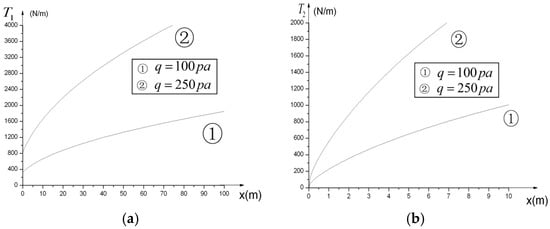
Figure 2.
Tension versus depth of parabolic membrane surface in longitudinal and latitudinal direction. (a) Tension in longitudinal direction; (b) Tension in latitudinal direction.
2.5. Ratios of Tension
According to Equations (13) and (21), the ratios of tension in two principal directions can be obtained in Equation (22), and the ratios’ limit of tension can be obtained in Equation (23).
As the membrane property of inflatable deployable parabolic membrane reflectors is isotropic thermoplastic polymer materials such as Kapton and Mylar, the stress ratio can affect the shape of reflectors and restrict wrinkling production and development from the unstress state to initial stress state; therefore, the stress ratio can decide the geometric design of inflatable deployable parabolic membrane reflectors. According to Equations (22) and (23), the stress ratio of tension in two directions of principal curvature on the parabolic membrane surface is independent of internal air pressure but is decided by the function of the parabolic membrane surface. As the depth of the parabolic membrane increases, the tension ratio gradually decreases and approaches 1/2. In the absence of other influencing factors, the wrinkles are minimized, the precision is maximized, and the mechanical and electromagnetic performance of the parabolic antenna is significantly enhanced [23,24,25,26,27].
Tension can be initially applied to the edge of inflatable deployable parabolic membranes and be delivered to the skirt edge of the membrane surface and inflated membrane ring with high pressure. Therefore, the tension at the equilibrium point can decide the outer ring, stress at the joint point and design of membrane antenna structures. Figure 3 shows the force analysis of the parabolic membrane surface at the edge of the skirt. Tensions at the up and down edges of antenna aperture of membrane surface are named as and ; their corresponding angles are and respectively as shown in Figure 3a. Therefore, for the tension force at the edge of the skirt, Equation (24) can be obtained based on equilibrium relationship of tension in the horizontal direction as shown in Figure 3.
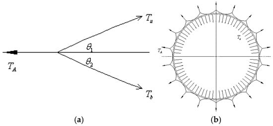
Figure 3.
Force analysis of parabolic membrane surface at the edge of the skirt. (a) Local schematic diagram; (b) Global diagram.
Due to symmetry of membrane surface and cables, membrane tension = = ; it can be simplified as Equation (25):
Therefore, tension at different points of membrane surface can increase as antenna aperture of membrane surface increases.
2.6. Deformation of the Reflector
Inflatable deployable parabolic membrane reflectors can be run normally based on deployment, lifespan and performance. Its performance could depend on the shape precision of membrane antenna structures. As shape precision of structure surface can affect signal reception and transmission, inflatable deployable reflectors must be manufactured as inflatable structures in a high accuracy. In this section, deformation at any point on the parabolic membrane surface under internal fixed air pressure can be obtained based on the non-momental theory of shell. Figure 4 shows parabolic membrane structure models. Geographical coordinates are used as the coordinates of the parabolic antenna. According to Figure 4a, differential field ABCD can be created by orthogonalizing two neighboring longitudes and latitude lines on the parabolic membrane models. The longitude is taken as the α line and the parallel circular is taken as the β line, which are, respectively, equal to φ and θ. φ is the supplementary angle of latitude measured from the axis of rotation, whereas θ is the longitude measured from any radius of parallel circular. Radius of curvature of the longitude is one of the principal curvature radii of any point on the surface; Ck1 can be considered as the radius of curvature r1 in accordance with Figure 4a. The circular center of the other principal curvature radius r2 is on the rotation axis and its direction is in the outer normal direction; therefore, Bk2 is considered as the other principal curvature radius , as shown in Figure 4a. According to Figure 4a, the radius r of parallel circular can be obtained in Equation (26):
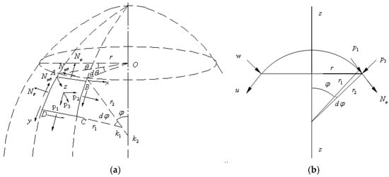
Figure 4.
Parabolic membrane model. (a) Symmetric shell model; (b) Parabola model in sectional view.
In Figure 4a, Nφ is tension force in the longitudinal direction, Nθ is the corresponding tension force in the other principal curvature direction. Therefore, Nφ = T1, Nθ = T2. , and are the components of force of any point on the parabolic membrane surface under external loads.
Figure 4b shows the parabola membrane model in a sectional view. As the reflector is created by rotating parabola considered as the generation line and the original point of coordinate axis (,) of the generation line is decided on the generation line, the parabola equation can be obtained in Equation (27):
According to Figure 4b, r1 and r2 are, respectively, the two principal radii of curvature at any point on the parabolic membrane surface. φ is the supplementary angle of latitude. u, v and w are displacements at any point on the parabolic membrane surface under the pressures of , and in their corresponding directions. As deformation of the rotational symmetry shell is symmetric, internal forces are independent of θ under external pressure p3 = −q. According to Equations (13) and (21):
According to Equations (27), (28) and r′ = ctgφ, Equation (29) can be obtained:
Taking Equation (29) into Equation (28), the tension forces in two principal directions can therefore be related to the variable φ in Equation (30):
The physical equation and geometric equation of the rotational symmetric shell can be, respectively, obtained in Equations (31) and (32):
As Nφθ = γφθ = 0 in the case of axisymmetric deformation, displacement component v and its corresponding derivative of θ are zero. Therefore, Equation (31) can be changed into Equation (33) as the third equation in Equation (31) is identically equal.
Therefore, Equation (34) can be obtained by using Equation (33):
Therefore, Equation (35) can be obtained:
where is a constant based on displacement boundary condition. For ω, it can be obtained by solving Equation (33). Therefore,
According to Equations (35) and (36), Equation (37) can be obtained:
According to Equations (33) and (37), Equation (38) can be obtained:
When the boundary condition is fixed, u = 0 on the edge of the boundary. As , according to parameters of the parabolic membrane surface, Equation (39) can be solved:
Therefore, Equations (40) and (41) can be obtained:
For the membrane material of Kapton, thickness of membrane h = 50 μm, Poisson’s ratio μ = 0.34 and tensile modulus E = 250 GPa. Figure 5 shows the deformation of any point on the parabolic antenna. According to parameters of the prototype antenna, the deformation u and w curves of the parabolic membrane surface with φ increases as shown in Figure 5.
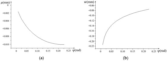
Figure 5.
Deformation of any point on the parabolic antenna. (a) u-φ; (b) ω-φ.
3. Precision Analysis
The effective aperture and reflector precision (root mean square) are key factors that could determine the characteristics of the parabolic antenna. The design of inflatable deployable parabolic membrane structures must meet the basic requirement of high surface accuracy, whereas some deviation exists between the actual configuration and ideal parabolic membrane surface. Therefore, the precision of parabolic antennas can affect their performance [28,29]. There are two forming methods to manufacture parabolic antennas. One is the monolithic casting form, and the other is gluing the sectioned membrane surfaces into one entire parabolic membrane surface based on the ideal parabolic surface. The essence of the second method is to approximate the non-deployable surface by using the deployable surface [30,31]. In this section, an experiment for a scaled-down inflatable parabolic membrane reflector is performed to study the precision of an inflatable parabolic antenna under various internal air pressures. To accurately measure the overall shape of parabolic membrane reflector and to examine the effectiveness of the production process, a phase and stereo vision technology is combined to scan the shape of the inflatable parabolic membrane reflector. By measuring the wrinkling of the overall parabolic membrane reflector including the longitudinal bonded seam, skirt, edge and corner of the skirt and junction point of the reflector, the mechanical characteristics of reflectors can be explored.
3.1. Experiments
Figure 6 shows experiments of the inflatable parabolic membrane reflector under various internal air pressures. The parabolic equation of the prototype model reflector is x2 + y2 = 13,212.619z as shown in Figure 1, whereas the parabolic equation of a scaled-down prototype model reflector is x2 + y2 = 1468.07z as shown in Figure 6a. In this experiment, the aperture and depth of antenna are, respectively, 1000 mm and 170.292 mm, which can be supported by ∅50 × 1.5 hollow stainless-steel tubes, as shown in Figure 6a. The inflatable parabolic membrane reflector with skirts and supporting hollow stainless-steel rings are octadecagon, as shown in Figure 6a. The reflector is constructed by seaming 18 membrane segments.
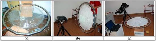
Figure 6.
Experiments of the inflatable parabolic membrane reflector. (a) Prototype; (b) A vertical test; (c) A horizontal test.
According to Figure 6b,c, the parabolic membrane reflector could be tested in vertical and horizontal states under various internal pressures. In these experiments, the internal air pressures of the parabolic antennas are, respectively, controlled at the magnitudes of 0 pa, 1 pa, 3 pa, 5 pa and 7 pa. Because the air pressure meter fluctuates during inflation, the antenna must be kept inflated until the internal pressure stabilizes. In these tests, the antenna should remain static for each internal air pressure in order to keep the parabolic surface in one same coordinate system. Then the parabolic membrane surfaces are, respectively, scanned by an OKIO-V-400 three-dimension scanner from a company named Beijing Ten Youn 3D Technology limited company. This device employs a white light scanning technique that combines phase-shifting and stereo vision technologies, allowing for precise measurement of the overall surface profile. The images are transmitted to a computer for result output, with a measurement accuracy of 0.025–0.04 mm.
3.2. Scanning Results
Scanning sketches of parabolic membrane surfaces in horizontal and vertical states under various pressures are, respectively, shown in Figure 7 and Figure 8. According to Figure 7, there are five scanning sketches of parabolic antennas in horizontal states under 0 Pa, 1 Pa, 3 Pa, 5 Pa and 7 Pa. It can be found that the parabolic membrane surface varies more and more tensely, and wrinkling reduces slowly as internal air pressure increases gradually. The wrinkling on the skirts reduces gradually with the skirts becoming more and more tight in the top center of the parabolic membrane surface, wrinkling also reduces as pressure increases; however, the wrinkling in the top center of the antenna can be observed more obviously than that in the other area of the antenna as internal air pressure increases, as shown in Figure 7. According to Figure 8, the wrinkling on the skirt and surface reduces gradually as internal air pressure increases. By comparing Figure 7 and Figure 8, as gravity of the parabolic membrane antenna distributes very uniformly in horizontal states but distributes unevenly in vertical states, it can be concluded that the wrinkling distributes uniformly in horizontal states, whereas wrinkling distributes more for the upper antenna than that for the bottom antenna in vertical states. However, the wrinkling in the center of the parabolic membrane surface can be observed more obviously than that in the other area as internal air pressure increases, as shown in Figure 7 and Figure 8. It can be inferred that the stress ratio of tension in two directions of principal curvature on the parabolic membrane surface is independent of internal air pressure according to Equations (22) and (23) and can infinitely converge to 1/2. As it gradually approaches 1/2, the surface wrinkles decrease, and the electromagnetic performance of the parabolic antenna is significantly enhanced.
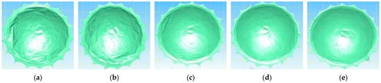
Figure 7.
Scanning sketches of parabolic membrane surfaces in horizontal states under various pressures. (a) 0 Pa; (b) 1 Pa; (c) 3 Pa; (d) 5 Pa; (e) 7 Pa.
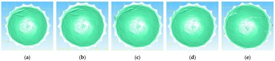
Figure 8.
Scanning sketches of parabolic membrane surfaces in vertical states under various pressures. (a) 0 Pa; (b) 1 Pa; (c) 3 Pa; (d) 5 Pa; (e) 7 Pa.
3.3. Result
As the parabolic membrane surfaces can be scanned into an electronic image with millions of points, a part of the points is selected as a reference point for surface fitting to simplify the calculation process. Figure 9 shows the point selection method of parabolic membrane surfaces for surface fitting. According to Figure 9, as picking point coordinates in eight directions of the parabolic membrane surface is a uniform point selection method for surface fitting, fitting results can roundly and effectively reflect the comprehensiveness of the parabolic membrane surface by using the function of polynomial fit type in the MATLAB R2010a software. The standard equation of the parabolic membrane surface is F(x,y) = −0.000681x2 − 0.000681y2. Table 1 describes the root mean square between the fitting curves and standard curves of the parabolic membrane surface in horizontal and vertical placement states under various pressures. The fitting equations and mean-fitting variances of the parabolic membrane surface in horizontal and vertical placement states under various pressures are, respectively, shown in Table 1. According to Table 1, as the coefficients of x2 and y2 of fitting equations are equal each other, the inflated parabolic antennas are close to paraboloid. As the mean fitting variances of fitting equations of parabolic antennas are under the pressure of 3 Pa in horizontal placement and under the pressure of 7 Pa in vertical placement, the parabolic membrane surface under the pressure of 3 Pa in horizontal placement and under the pressure of 7 Pa in vertical placement are, respectively, closest to the standard parabolic surface. By comparing the root mean squares between fitting curves and standard curves, it can be concluded that the loading states of the closest fitting equations of parabolic antennas are, respectively, under the pressures of 7 Pa in horizontal states and of 5 Pa in vertical states as their RMSs are, respectively, minimum in accordance with Table 1.
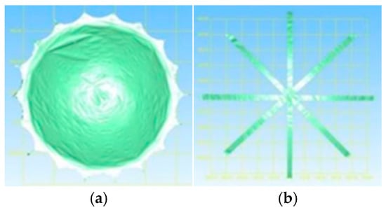
Figure 9.
Point selection method of parabolic membrane surfaces for surface fitting. (a) An electronic image; (b) Point selection for surface fitting.

Table 1.
RMSs between fitting curves and standard curves of parabolic membrane surface in horizontal and vertical placement states under various pressures.
4. Numerical Analysis
4.1. Modal Analysis
As the posture of inflatable deployable antennas should be adjusted to enter their working orbit under operation condition, dynamic responses of parabolic antennas should be performed as a key point. The basic content of dynamic responses is modal analysis, which decides natural frequencies and mode shapes. If the natural frequencies and mode shapes of the structures are known, the structures can avoid resonance at the stage of design once the loading frequency can be obtained [32,33]. In this section, the free vibration characteristics of parabolic antennas including supporting rings, parabolic membrane surface, skirts and cables are proposed; then, modal analysis and transient responses of global antenna models with various boundary conditions are also performed.
Natural frequencies and the corresponding mode shapes of the structures can represent the free vibration characteristics of membrane antenna structures; the multi degree of freedom undamped free vibration equation can be a generalized eigenvalue problem. Modal analysis of the inflatable deployable parabolic membrane surface should be applied prestress due to flexibility of the structure whereas the posture of the parabolic antenna should be adjusted after its hardening; therefore, the flexible membrane system can transfer into a flexible thin-walled system. In this section, the modal analysis of global and local parts of the parabolic antenna should be performed numerically by using shell elements not considering prestress.
4.1.1. Principles
According to the Hamilton variational principle, the free vibration equilibrium equation of structures not considering external loading and damping action can be obtained:
where is the mass matrix of structures, is the stiffness matrix of structures, is the amplitude vector of node.
The generalized eigenvalue equation can be obtained by transferring Equation (42):
where is the circular frequency of structure vibration and is the eigenvector.
Generalized eigenvalue solution includes the subspace iteration method, Lanczos method, householder method, asymmetric method, and damping method; the Lanczos method is used in this section for modal analysis.
4.1.2. Numerical Models
Figure 10 shows the finite element models of the parabolic antenna including the supporting ring, parabolic surface and parabolic membrane reflector without constraint and parabolic membrane reflector with three constrained cross sections. Two adjacent hollow tubes are intersected with each other forming the supporting ring, as shown in Figure 10. The diameter of one tube is 150 mm and radius of the incircle in the supporting ring is 1670 mm. The boundary condition of FE models is free in Figure 10a–c, whereas three cross sections of the parabolic antenna are constrained in Figure 10d. The material properties of parabolic antennas are shown in Table 2. For the parabolic antenna, it can be composed of a symmetric parabolic surface and reflector, the skirts connected to the edge of the reflector, and the edge cables connected to the skirts and tension cables, as shown in Figure 10. To study the vibration characteristics of the hardened parabolic antenna, the membrane structure and edge cables and tension cables should be numerically simulated in the ABAQUS 6.8 software. The models are simulated as ideal parabolic antennas and their protype equation is x2 + y2 = 13,212.619z as shown in Figure 1.
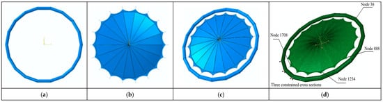
Figure 10.
Finite element models of parabolic antenna. (a) Supporting ring; (b) parabolic surface; (c) parabolic reflector; (d) Model with three cross sections.
Table 2.
Material properties and geometric data of parabolic antenna.
4.1.3. Vibration Characteristics
As shown in Figure 11, after the inflatable structure is fully deployed in space, it undergoes a hardening process to become rigid, eliminating the need for continuous inflation to maintain its shape. In the modal analysis of the hardened supporting ring, shell elements are utilized, with the boundary condition set to free. For this analysis in ABAQUS, a total of 9720 S4R5 shell elements are used to model the supporting ring. As shown in Figure 12, similar to the analysis of the supporting ring, the modal analysis of the reflector structure is also performed after it has been hardened. Therefore, shell elements are used for modeling, and the edge cables and tendons are modeled using BEAM elements. Both the reflector surface and the incident surface use the S4R5 element type, with a total of 9900 elements. Due to the irregular shape of the skirt, S3 elements are used to ensure uniformity in element shape and size, with a total of 436 elements. The edge cables and tendons are modeled using B31 elements, with 180 and 90 elements, respectively. The boundary conditions are set by restraining all translational degrees of freedom at the outer endpoints of 18 segments of the tendons. As shown in Figure 13, since the analysis involves the antenna structure’s free vibration modes after hardening, all the original membrane components are modeled using shell elements, while the edge cables and tendons are modeled using BEAM elements. Both the reflector surface and the incident surface use the S4R5 element type, with a total of 9900 elements. The skirt is modeled using S3 elements, with a total of 436 elements. The edge cables and tendons are modeled using B31 elements, with 180 and 90 elements, respectively. The supporting ring uses the S4R5 element type, with a total of 9720 elements. The boundary conditions are set to free, meaning that the structure is unconstrained. Figure 11 shows the mode shapes of supporting rings and Table 3 describes the natural frequencies of supporting rings. It can be found that as supporting rings under a free boundary condition are central symmetric structures around a circular center, mode shapes occur from the 7th mode, and the two adjacent modes are symmetric, and their corresponding frequencies are equal to each other. Mode shapes of the parabolic membrane surface are shown in Figure 12 and corresponding natural frequencies of the parabolic membrane surface are shown in Table 4. According to Figure 12, the 1st, 2nd and 4th mode shapes and corresponding frequencies of the parabolic membrane surface are independent of each other whereas other mode shapes and frequencies are not independent. The 2nd and 3rd mode shapes are symmetric in Figure 12 and corresponding frequencies are equal each other in Table 4. The other mode shapes, from the 5th mode, are all close to the 4th mode, and corresponding frequencies are all equal to about 4.0. Figure 13 shows the mode shapes of the parabolic membrane surface, and Table 5 displays the natural frequencies of the parabolic antenna. According to Figure 13, the first six modes are rigid modes due to the free boundary condition of the structure. Two adjacent modes are symmetric since 7th modes due to symmetry of the parabolic antenna. The vibration modes are similar from the 14th mode. By comparing Figure 11, Figure 12 and Figure 13, the 7th, 8th and 9th modes occur mainly based on the vibration of the reflector whereas the 10th to 13th modes are mainly caused by vibrations of the supporting ring. However, their frequencies are lower than those of the independent reflector and independent supporting ring. From the 14th mode, the mode shapes of the global parabolic antenna begin to correspond with the 4th mode of the independent parabolic membrane surface, according to Figure 12d and Figure 13e, and the corresponding frequencies are close each other. For low-level vibrations, the frequencies of the global parabolic antenna are close to those of the independent supporting ring such as the 7th frequency of 0.601 and 8th frequency of 0.742. It can also be found that the 7th frequency (0.971) of the supporting ring reduces the 1st frequency (0.224) and is approximately equal to the 8th and 9th frequencies of the global parabolic antenna, according to Table 3, Table 4 and Table 5.
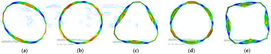
Figure 11.
Mode shapes of supporting rings. (a) 7th modes; (b) 9th modes; (c) 11th modes; (d) 13th modes; (e) 15th modes.
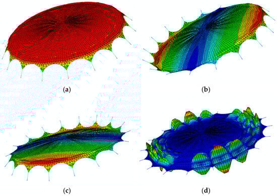
Figure 12.
Mode shapes of parabolic membrane surface. (a) 1st mode; (b) 2nd mode; (c) 3rd mode; (d) 4th mode.
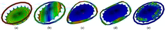
Figure 13.
Mode shapes of parabolic membrane reflector including surface and supporting rings. (a) 7th mode; (b) 8th mode; (c) 10th mode; (d) 12th mode; (e) 14th mode.
Table 3.
Natural frequencies of supporting rings (Hz).
Table 4.
Natural frequencies of parabolic membrane surface (Hz).
Table 5.
Natural frequencies of parabolic membrane reflector (Hz).
4.2. Analysis of Transient Response
4.2.1. Methods
The transient response can be numerically studied by three methods: the full method, reduced method and mode superposition method [34,35,36]. The transient response could be calculated by using a complete system matrix based on the full method involving various nonlinear characteristics of plasticity, large deformation and large strain. The reduced method is used by decreasing the matrix and degrees of freedom to calculate the transient response. The mode superposition method is used to sum the corresponding eigenvalues of mode shape multiplying coefficients in order to obtain the transient response. However, the computational efficiency of the mode superposition method is higher than the full method and reduced method and mode damping can also be considered by the mode superposition method. In this section, the mode superposition method is adopted to study the transient response of the parabolic antenna. Firstly, the actual eigenvalue analysis can be performed by ignoring the damping to obtain the modal vector. Then, to obtain the imaginary eigenvalues, the generalized mass matrix, generalized stiffness matrix and generalized damping matrix can be obtained by using generalized modal coordinates to form a structural governing equation.
When the dynamic response of the model can be expressed by the eigenvectors, the function of time t can be obtained as follows:
where , represent the eigen interval. is the transformation matrix of the viscous damping matrix. is the generalized coordinates of mode (a response amplitude in mode ). is the natural frequency of the undamped mode. is loading amplitude mapped to the mode . is the variation in f in the time period of .
If the transformation matrix of the damping matrix is the diagonal matrix, Equation (44) can be changed into Equation (45):
where is the critical damping ratio; therefore, Equation (46) can be obtained:
where and are, respectively, the mode viscous damping coefficient and mode mass.
When composite mode damping is used, the mode damping of each material is a fraction of the critical damping of the composite material; then, the mode damping values of all the materials in each corresponding mode vector direction is combined into one weighted average. The weight can be obtained by the mass matrix Equation (47):
where is the critical damping ratio in mode , is the critical material percentage defined based on the material , is the mass matrix related to material , is the eigenvalues of αth mode, and is the generalized mass matrix related to αth mode ().
4.2.2. Extraction of Natural Vibration
To study the transient response of the parabolic antenna, the natural vibration including natural frequencies and their corresponding mode shapes of the parabolic membrane should be extracted. The material property and geometrical data of the parabolic antenna can be obtained in Table 2. The numerical simulation is performed using ABAQUS finite element software, with the same element types and quantities as those used in Figure 13. The boundary conditions are shown in Figure 10d, where the three adjacent cross sections of the hollow tubes in the finite element model are fully fixed. The results of the natural frequency extraction are shown in Table 6, and the first few modes are shown in Figure 14.
Table 6.
The first twenty frequencies of the parabolic antenna with constraint (Hz).
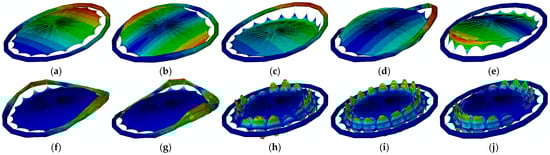
Figure 14.
Ten mode shapes of parabolic antenna with constraint. (a) Mode 1; (b) Mode 2; (c) Mode 3; (d) Mode 4; (e) Mode 5; (f) Mode 6; (g) Mode 7; (h) Mode 8; (i) Mode 10; (j) Mode 14.
4.2.3. Transient Response
Based on the natural vibration characteristics, the transient response of this parabolic antenna should be obtained by considering the critical damping ratios of 1%, 2% and 5%. The magnitudes of the acceleration versus time curves under translational acceleration and rotational acceleration around the x- and y-axes are shown in Figure 15. Then, as the maximum frequency of the selected modes is 4.06 Hz, as shown in Table 6, and its corresponding period is 1/4.06 = 0.246s, and time increment of step of transient response needs be less than the period, the selected time increment is 0.05 s. The time duration of external excitation is 4.8 s; as the vibration response lasts a long time, the time duration of step of transient response is selected as 200 s to observe the attenuation process of fluctuation. In this section, the transient response of the parabolic antenna under three control signals can be obtained.
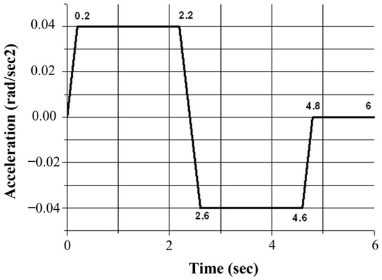
Figure 15.
Control signals under translational acceleration, rotational acceleration around x- and y-axes.
According to Figure 15 and Figure 16, the total kinetic energies and displacements of the parabolic antenna under pulsing translational acceleration with a peak magnitude of 0.1G damply fluctuate to 0 J in the process of attenuation. The greater the damping of structures, the faster the velocity of attenuation including displacement. Maximum displacements for the critical damping ratios of 2% and 5% attenuate to 0 mm within 200 s and 75 s, respectively, according to Figure 16. Maximum displacement and stress, respectively, occur at node 38 on the outer supporting rings and at node 1234 in the vicinity of the edge cable on the skirt edge, as shown in Figure 10d. Maximum stresses of the critical damping ratios of 1%, 2% and 5%, respectively, damply fluctuate from 0.1772 MPa to 2.929 × 10⁻³ MPa, from 0.1715 MPa to 1.834 × 10⁻⁴ MPa and from 0.1564 MPa to 5.037 × 10⁻⁸ MPa within 200 s.
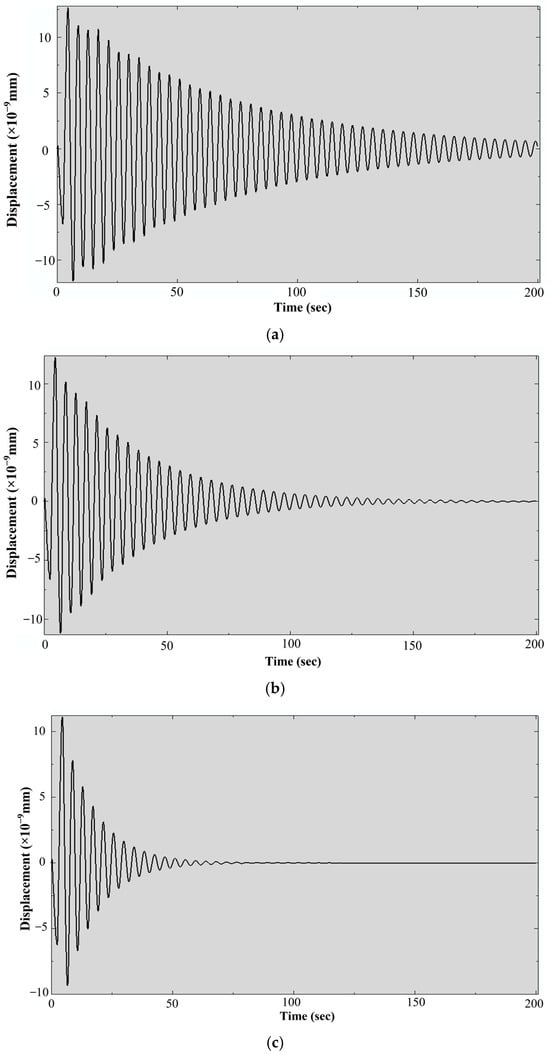
Figure 16.
Displacement amplitude attenuation of the structures under critical damping ratios. (a) 1%; (b) 2%; (c) 5%.
The transient response under pulsing rotational acceleration with a peak magnitude of 0.04 rad/s2 around the x-axis and y-axis gradually decayed to 0 J, including displacement. It can be concluded that the velocity of attenuation, including displacement, increases as damping of the structure increases. Maximum displacement of the parabolic antenna could gradually reduce from the parabolic antenna from 2.46 × 10⁻⁸ mm to 0.18 × 10⁻⁸ mm during 200 s for the case of 1%, and maximum displacement of the structures varies from 2.35 × 10⁻⁸ mm to 0 mm at the time of 200 s for the critical damping ratio of 2%, whereas the attenuation of maximum displacement of the structures for the case of 5% from 2.05 mm to 0 mm only cost 80 s. Maximum displacement and stress of the structures exist, respectively, at nodes 38 and 888, as shown in Figure 10d. The attenuations of maximum stress of the structures vary, respectively, from a maximum of 2.01 × 10⁻⁹ MPa to 1.396 × 10⁻¹¹ MPa, 1.994 × 10⁻⁹ MPa to 8.777 × 10⁻¹³ MPa and 1.943 × 10⁻⁹ MPa to 2.410 × 10⁻¹⁶ MPa for the critical damping ratios of 1%, 2% and 5% within 200 s. Maximum displacements of the parabolic antenna for the critical damping ratios of 1% and 2%, respectively, decay from 4.26 × 10⁻⁸ mm to 0.345 × 10⁻⁸ mm and from 4.03 × 10⁻⁸ mm to 0 mm within 200 s, whereas for the case of 5%, its maximum displacement reduces from 3.74 mm to 0 mm only during the time of 80 s. Maximum displacement and stress occur at nodes 38 and 1708, as shown in Figure 10d. For stress attenuations, they, respectively, change from 2.383 × 10⁻⁹ MPa to 2.165 × 10⁻¹¹ MPa, from 2.353 × 10⁻⁹ MPa to 1.367 × 10⁻¹² MPa and from 2.266 × 10⁻⁹ MPa to 3.754 × 10⁻¹⁶ MPa within 200 s. Therefore, it can be obtained that maximum stress and maximum displacement of the parabolic antenna under translational acceleration is 108, 1016 and 108 times than those of the parabolic antenna under rotational acceleration. Thus, the effect of pulsing translational acceleration on the stability of the parabolic antenna is greater than that of rotational acceleration around the x- and y-axes. As the attenuation velocities of the mechanical characteristics of the parabolic antenna are faster as the damping of the structures increases, the structural damping should be increased properly to reduce the negative effect of external perturbance on the stability of the parabolic antenna.
5. Conclusions
In this paper, the mechanical characteristics of the parabolic membrane surface can be studied to explore the force analysis, precision analysis and transient responses of the parabolic antenna under various internal pressures. Analytical solutions of the parabolic antenna have been proposed to obtain the theoretical solution of force analysis on the parabolic membrane surface. It can be concluded that the stress ratio of tension in two directions of principal curvature on the parabolic membrane surface is independent of internal air pressure but is decided by the function of the parabolic membrane surface. The ratio of tension reduces as depth of the parabolic membrane increases and can infinitely converge to 1/2. As the tension ratio gradually approaches 1/2, the wrinkles reach their minimum under ideal conditions.
- For precision analysis, as gravity of the parabolic membrane reflector in horizontal placement distributes uniformly, its winkling distributes uniformly. Conversely, the parabolic membrane surface wrinkles unevenly in vertical placement, and the amount of wrinkling on the lower part of the reflector are more than those on the upper part of the reflector. In this paper, the antenna aperture is very small, and the curvature of the parabolic membrane surface is very large. The wrinkling is much more noticeable compared to that of an antenna with a larger aperture. As a result, the deviation between the fitted parabolic surface equation and the design equation is significant. According to the comparison between the fitting parabolic surface equation and design equation, precision of the parabolic membrane surface in a vertical state is higher than that in a horizontal state. At a pressure of 5 Pa, the root mean square error between the fitted curve and the standard curve is 4.85, which is lower than in all other cases. At this point, the shape of the parabolic membrane surface is closest to the parabolic design equation.
- For transient response, natural vibration of the supporting rings and reflector of the parabolic antenna is performed; then, transient response of the parabolic antenna under pulsing control signal is proposed. It can be found that as supporting rings could affect the natural vibration of middle modes whereas the reflector could affect the natural vibration of lower and higher modes, the vibration characteristics of the supporting rings and reflector can be, respectively, adjusted to control the natural vibration of the parabolic antenna. For the same loading states, decay rates of the mechanical characteristics of the structures with damping of the structures increases. As stress and displacement of the inflatable parabolic antenna under translational acceleration is far greater than those under rotational acceleration, the effect of translational acceleration on the stability of the structures is far greater than the effect of rotational acceleration in terms of adjusting the posture of the inflatable parabolic antenna.
In this paper, the limitations of this study are as follows: (1) The results of the modal analysis and transient response have not been validated through experiments. (2) The analysis in this paper is conducted under ideal conditions, without considering the impact of factors such as temperature and air on the membrane structure.
Author Contributions
Conceptualization, Y.H.; methodology, Y.H.; software, Y.H.; validation, Y.H.; formal analysis, W.C.; investigation, Y.H.; resources, Y.H.; data curation, W.C.; writing—original draft preparation, Y.H.; writing—review and editing, H.J.; visualization, H.J.; supervision, H.J.; project administration, W.C.; funding acquisition, W.C. All authors have read and agreed to the published version of the manuscript.
Funding
The first author acknowledges with thanks the research financial support provided by the Wuhan Talent Project for Excellent Youth (No. 45222071).
Data Availability Statement
Data is available upon request to the corresponding authors.
Acknowledgments
All authors also would like to thank the anonymous reviewers for their constructive comments to improve the quality of the paper.
Conflicts of Interest
The authors declare no conflict of interest.
References
- Zhang, Y.Q.; Sun, Z.H.; Yang, D.W.; Du, J.H.; Li, N. Performance Coordination of Structure and Deployment Properties of Deployable Antenna. J. Aerosp. Eng. 2019, 32, 4019073. [Google Scholar] [CrossRef]
- Jiang, W. Design, Analysis and Experimental Researches for Space Inflatable Antenna Reflectors. Master’s Thesis, Shanghai Jiao Tong University, Shanghai, China, 2007. [Google Scholar]
- Venkata, S.P.; Balbi, V.; Destrade, M.; Zurlo, G. Designing necks and wrinkles in inflated auxetic membranes. Int. J. Mech. Sci. 2024, 268, 109031. [Google Scholar] [CrossRef]
- Tian, H.; Potier-Ferry, M.; Abed-Meraim, F. Buckling and wrinkling of thin membranes by using a numerical solver based on multivariate Taylor series. Int. J. Solids Struct. 2021, 230–231, 111165. [Google Scholar] [CrossRef]
- Adler, A.L. Finite Element Approaches for Static and Dynamic Analysis of Partially Wrinkled Membrane Structures. Ph.D. Thesis, University of Colorado, Boulder, CO, USA, 2000. [Google Scholar]
- Greschik, G.; Mikulas, M.M. Design Study of a Square Sail Architecture. In Proceedings of the 42nd AIAA/ASME/ASCE/AHS/ASC Structures Dynamics, and Material Conference and Exhibit, Seattle, WA, USA, 16–19 April 2001. AIAA-2001-1259. [Google Scholar]
- Liu, Z.Q.; Qiu, H.; Li, X.; Yang, S.L. Review of Large Spacecraft Deployable Membrane Antenna Structures. Chin. J. Mech. Eng. 2017, 30, 1447–1459. [Google Scholar] [CrossRef]
- Le Meitour, H.; Rio, G.; Laurent, H.; Lectez, A.; Guigue, P. Analysis of wrinkled membrane structures using a Plane Stress projection procedure and the Dynamic Relaxation method. Int. J. Solids Struct. 2021, 208, 194–213. [Google Scholar] [CrossRef]
- Lopez, B.; Lou, M.; Huang, J.; Edelstein, W. Development of an inflatable SAR engineering model. In Proceedings of the 19th AIAA Applied Aerodynamics Conference, Anaheim, CA, USA, 11–14 June 2001. [Google Scholar]
- Zhang, J.; Xu, W.; Yang, Z.; Guo, H.; Liu, R.; Kou, Z. Design and analysis of parabolic membrane crease inspired by origami. Thin-Walled Struct. 2022, 181, 110121. [Google Scholar] [CrossRef]
- Zhang, Z.; Li, J.; Wang, C.; Guang, C.; Ni, Y.; Zhang, D. Design and Optimization of Kirigami-inspired Rotational Parabolic Deployable Structures. Int. J. Mech. Sci. 2024, 263, 108788. [Google Scholar] [CrossRef]
- Li, Q.; Guo, X.; Qing, Q.; Gong, J. Dynamic deflation assessment of an air inflated membrane structure. Thin-Walled Struct. 2015, 94, 446–456. [Google Scholar] [CrossRef]
- Wang, X.; Fu, H.; Law, S.-S.; Yang, Q.; Yang, N. Experimental study on the interaction between inner air and enveloping membrane of inflated membrane tubes. Eng. Struct. 2020, 219, 110892. [Google Scholar] [CrossRef]
- Sun, X.Y.; Yu, R.T.; Wu, Y. Investigation on wind tunnel experiments of ridge-valley tensile membrane structures. Eng. Struct. 2019, 187, 280–298. [Google Scholar] [CrossRef]
- Liu, T.; Wang, X.; Qiu, X.; Zhang, X. Theoretical study on the parameter sensitivity over the mechanical states of inflatable membrane antenna. Aerosp. Sci. Technol. 2020, 102, 105843. [Google Scholar] [CrossRef]
- Samy, A.; Yuan, X.; Zhang, Y.; Zhang, W. Study on bagging effect and rupture failure of membrane structures. Eng. Struct. 2021, 232, 111880. [Google Scholar] [CrossRef]
- Liu, C.; Deng, X.; Liu, J.; Peng, T.; Yang, S.; Zheng, Z. Dynamic response of saddle membrane structure under hail impact. Eng. Struct. 2020, 214, 110597. [Google Scholar] [CrossRef]
- Wang, J.; Chen, D.; Zhang, Y.; Qian, H. Numerical method for the form finding and force analysis of non-prestressed cable-membrane structures with mechanism displacement. Eng. Struct. 2024, 311, 118173. [Google Scholar] [CrossRef]
- Zhong, W.; Gu, Y.; Yang, J. Modified crease-free design method for parabolic membrane considering unfolded structural performance. Adv. Space Res. 2025, 76, 1150–1162. [Google Scholar] [CrossRef]
- Liu, C.; Pan, R.; Deng, X.; Xie, H.; Liu, J.; Wang, X. Random vibration and structural reliability of composite hyperbolic–parabolic membrane structures under wind load. Thin-Walled Struct. 2022, 180, 109878. [Google Scholar] [CrossRef]
- Colin, J. Buckling and folding of a ductile thin film on a rigid substrate. Mech. Res. Commun. 2024, 135, 104237. [Google Scholar] [CrossRef]
- Li, D.; Zhu, Q.; Shen, R.; Lu, L.; Lai, Z. Random vibration response and reliability analysis of hyperbolic parabolic membrane structures under typhoons. Thin-Walled Struct. 2024, 205, 112444. [Google Scholar] [CrossRef]
- Zhang, S.; Baoyan, D.; Zhang, S.; Nan, W. Structural design and model fabrication of cable-rib tensioned deployable parabolic cylindrical antenna. Chin. J. Aeronaut. 2023, 36, 229–246. [Google Scholar] [CrossRef]
- Hang, X.; Shengnan, L.Y.U.; Xilun, D. Optimizing accuracy of a parabolic cylindrical deployable antenna mechanism based on stiffness analysis. Chin. J. Aeronaut. 2020, 33, 1562–1572. [Google Scholar] [CrossRef]
- Tang, R.; Meng, Q.; Liu, X.-J. Deployable support truss for parabolic cylindrical antennas with shape reconfiguration. Int. J. Mech. Sci. 2024, 278, 109419. [Google Scholar] [CrossRef]
- Li, M.; Zhu, K.; Qi, G.; Kang, Z.; Luo, Y. Wrinkled and wrinkle-free membranes. Int. J. Eng. Sci. 2021, 167, 103526. [Google Scholar] [CrossRef]
- Wang, X.F.; Law, S.S.; Yang, Q.S.; Yang, N. Numerical study on the dynamic properties of wrinkled membranes. Int. J. Solids Struct. 2018, 143, 125–143. [Google Scholar] [CrossRef]
- Xiao, W.W.; Chen, W.J.; Fu, G.Y. The Prestress Introduction Effect and Influencing Factors of Spatial Membrane Array. J. Astronaut. 2010, 31, 845–849. [Google Scholar]
- Xiao, W.W.; Chen, W.J.; Fu, G.Y. Analysis of the design and precision of an inflatable deployable parabolic reflector space antenna. J. Harbin Eng. Univ. 2010, 31, 257–261. (In Chinese) [Google Scholar]
- Galasko, G.; Leon, J.; Trompette, P.; Veron, P. Textile Structures: A Comparison of Several Cutting Pattern Methods. Int. J. Space Struct. 1997, 12, 9–18. [Google Scholar] [CrossRef]
- Freeland, R.E.; Bilyeu, G. In-step inflatable antenna experiment. Acta Astronaut. 1993, 30, 29–40. [Google Scholar] [CrossRef]
- Kawai, H.; Yoshie, R. Wind-induced response of a large cantilevered roof. J. Wind. Eng. Ind. Aerodyn. 1999, 83, 263–275. [Google Scholar] [CrossRef]
- Daw, D.J.; Davenport, A.G. Aerodynamic damping and stiffness of a semi-circular roof in turbulent wind. J. Wind. Eng. Ind. Aerodyn. 1989, 32, 83–92. [Google Scholar] [CrossRef]
- Yang, Q.; Wang, L.; Wang, J. Natural vibration analysis model of closed fabricstructures with openings. Spat. Struct. 2003, 9, 44–46. [Google Scholar]
- Yu, Z.; Zhao, L. Research on Free Vibration Properties of Membrane Structure. J. Southwest Jiaotng Univ. 2004, 39, 734–739. (In Chinese) [Google Scholar]
- Mao, G. Research on Design Methods of Cable Membrane Structures. Ph.D. Thesis, Zhejiang University, Hangzhou, China, 2004. Available online: https://d.wanfangdata.com.cn/thesis/Y600253 (accessed on 17 June 2025).
Disclaimer/Publisher’s Note: The statements, opinions and data contained in all publications are solely those of the individual author(s) and contributor(s) and not of MDPI and/or the editor(s). MDPI and/or the editor(s) disclaim responsibility for any injury to people or property resulting from any ideas, methods, instructions or products referred to in the content. |
© 2025 by the authors. Licensee MDPI, Basel, Switzerland. This article is an open access article distributed under the terms and conditions of the Creative Commons Attribution (CC BY) license (https://creativecommons.org/licenses/by/4.0/).