Optimization of Test Mass Motion State for Enhancing Stiffness Identification Performance in Space Gravitational Wave Detection

Abstract

In space gravitational wave detection, various physical effects in the spacecraft, such as self-gravity, electricity, and magnetism, will introduce undesirable parasitic stiffness. The coupling noise between stiffness and the motion states of the test mass critically affects the performance of scientific detection, making accurate stiffness identification crucial. In response to the question, this paper proposes a method to optimize the test mass motion state for enhancing stiffness identification performance. First, the dynamics of the test mass are studied and a recursive least squares algorithm is applied for the implementation of on-orbit stiffness identification. Then, the motion state of the test mass is parametrically characterized by multi-frequency sinusoidal signals as the variable to be optimized, with the optimization objectives and constraints of stiffness identification defined based on convergence time, convergence accuracy, and engineering requirements. To tackle the dual-objective, computationally expensive nature of the problem, a multigranularity surrogate-assisted evolutionary algorithm with individual progressive constraints (MGSAEA-IPC) is proposed. A fuzzy radial basis function neural network PID (FRBF-PID) controller is also designed to address complex control needs under varying motion states. Numerical simulations demonstrate that the convergence time after optimization is less than 2 min, and the convergence accuracy is less than 1.5 × 10⁻¹⁰ s⁻². This study can provide ideas and design references for subsequent related identification and control missions.

1. Introduction

Gravitational waves are ripples in space-time caused by some of the most violent and energetic processes in the universe and provide a new means of observation for exploring the unknown universe [1,2,3]. Currently, space gravitational wave detection projects being researched include LISA [4], ‘Taiji’ [5], and ‘Tianqin’ [6], with the LISA Pathfinder (LPF) [7], ‘Taiji-1’ [8], and ‘Tianqin-1’ [9] achieving significant advancements in key technology.

Space gravitational wave detection adopts the laser interferometry method, using the three-satellite formation in space to detect the distance changes of picometre-scale low-frequency (0.1 mHz~1 Hz) between test masses with baselines of more than 10⁵ km caused by gravitational waves [10]. The detection sensitivity needs to reach the order of 10⁻²¹, which corresponds to the requirements of achieving a laser interferometry optical distance noise of better than the order of 10⁻¹² m/Hz^1/2 and a test mass residual acceleration noise of better than the order of 10⁻¹⁵ m/s²/Hz^1/2. For this purpose, it is necessary to keep the test mass in free suspension by drag-free control and maintain an ultra-low level of residual acceleration as an inertial reference for laser interferometry.

The residual acceleration noise of the test mass is mainly composed of direct and displacement-coupled disturbances to the test mass [11]. The direct disturbances include magnetic field disturbances, cosmic rays, residual gases, temperature rise and fall, etc., while the displacement-coupled disturbances are due to the coupling of the relative displacement noise introduced by the displacement sensing and control loops and the parasitic stiffness between the test mass and the spacecraft, which in turn generates acceleration disturbances acting on the test mass.

It is particularly important to point out that the parasitic stiffness in space gravitational wave detection is different from the conventional concept of stiffness. Conventional stiffness usually refers to the ability of a material or structure to resist elastic deformation when subjected to force, which is closely related to the elastic modulus, geometry, and boundary conditions of the material. This is common in fields such as robotics [12], materials [13], and building structures [14]. However, the stiffness mentioned in this paper mainly originates from the spatial gradient of the disturbance force, which is caused by various physical effects in the spacecraft. For the convenience of representation, this parasitic stiffness is described in this paper as the test mass stiffness, which may be negative due to the spacecraft device characteristics, drive configuration, and other factors. The test mass stiffness is mainly composed of self-gravity stiffness, magnetic stiffness, and electrostatic stiffness. During actual operation, the stiffness changes caused by the above factors are negligible compared to the nominal value [15,16]. Therefore, the stiffness can be viewed as a constant parameter within a single calibration cycle. However, due to possible long-term drift, periodic online calibration may still need to be considered.

Test mass stiffness and displacement coupling noise, as an important component of residual acceleration noise, greatly affects the performance of space gravitational wave detection. It is necessary to accurately identify the stiffness to verify and optimize the control effect [17,18,19] and achieve noise suppression. For the gravitational wave detection mission, the accuracy of stiffness identification should reach at least the order of 10⁻⁸ s⁻². Fast convergence is also necessary to prevent unknown risks caused by long-term signal injection. Ziegler T and Fichter W [20] implemented on-orbit stiffness identification of an LPF test mass by combining least squares and instrumental variable identification methods from the differential dynamics of the spacecraft and test mass, with an identification accuracy of 2–3%. Nofrarias M et al. [21] used a Bayesian framework for identifying simplified model parameters of the LISA technology package instrument, including stiffness, gain coefficients, etc. The results showed that the method achieved the best achievable error, which was the Cramér-Rao bound. Congedo G et al. [22] proposed a time-domain maximum likelihood parameter estimation method to accurately calibrate LPF key system parameters from the perspective of data analysis. The validity was verified by Monte Carlo implementation of independent noise runs, where the average standard deviation of the stiffness was better than the order of 10⁻⁹ s⁻². Armano M et al. [23] used an iterative reweighted least squares algorithm to achieve on-orbit identification of system dynamics parameters such as LPF test mass stiffness, electrostatic gain coefficient, etc., and discussed their importance for future LISA missions.

In the LPF mission, the two test masses adopt a coaxial layout. However, for space gravitational wave detection programs such as LISA, ‘Taiji’, and ‘Tianqin’, the two test masses adopt a non-coaxial and V-shaped layout. This configuration not only increases the complexity of dynamics but also puts forward higher requirements on the processing of the related disturbance. This leads to the fact that the stiffness identification method in the LPF mission is not completely applicable for space gravitational wave detection. In this paper, we investigate the stiffness identification and performance enhancement in the non-coaxial case. Since we have already done some work on identification before [24], with a root mean square error (RMSE) of stiffness identification of less than 1.5 × 10⁻⁸ s⁻², this paper mainly focuses on enhancing the stiffness identification performance as high as possible without paying other expensive costs in the ground simulation stage to provide a margin for future on-orbit realization.

In the process of parameter identification, the applied excitation signal has an important influence on identification performance. An appropriate excitation signal can improve the observability of system response and thus effectively identify system parameters [25,26]. In recent years, researchers in different fields have proposed a variety of methods to optimize identification performance based on different excitation strategies and combined them with modern algorithms, such as evolutionary algorithms, neural networks, and deterministic learning, for further research [27,28,29,30,31]. For the problem of identifying the test mass stiffness in space gravitational wave detection, evolutionary algorithms are chosen as optimization tools that can effectively handle multi-peaks and high-dimensional search spaces in excitation signal optimization and do not rely on the calculation of gradient information. Inspired by the above, this paper proposes a method to optimize the test mass motion state for enhancing stiffness identification performance, including the convergence time and convergence accuracy, where the motion state in the form of a multi-frequency sinusoidal signal serves as the excitation signal. A multigranularity surrogate-assisted evolutionary algorithm with individual progressive constraints (MGSAEA-IPC) is proposed based on the characteristics of dual-individual, expensive objectives and the constraints of the optimization problem. In addition, to meet complex control requirements under different motion states, a fuzzy radial basis function neural network PID (FRBF-PID) controller is designed. Numerical simulation experiments demonstrate that our method is effective, and this study can provide ideas and design references for subsequent related identification and control missions.

The rest of this paper is organized as follows. Section 2 presents the basic principles of test mass stiffness identification. Section 3 describes the methods for enhancing the performance of stiffness identification, including the definition of the optimization problem, the proposal of a targeted optimization algorithm, and the controller design. Section 4 conducts numerical simulation experiments and result analyses to verify the effectiveness of the methods proposed in this paper. Finally, Section 5 presents the conclusion to the paper.

2. Principle of Test Mass Stiffness Identification

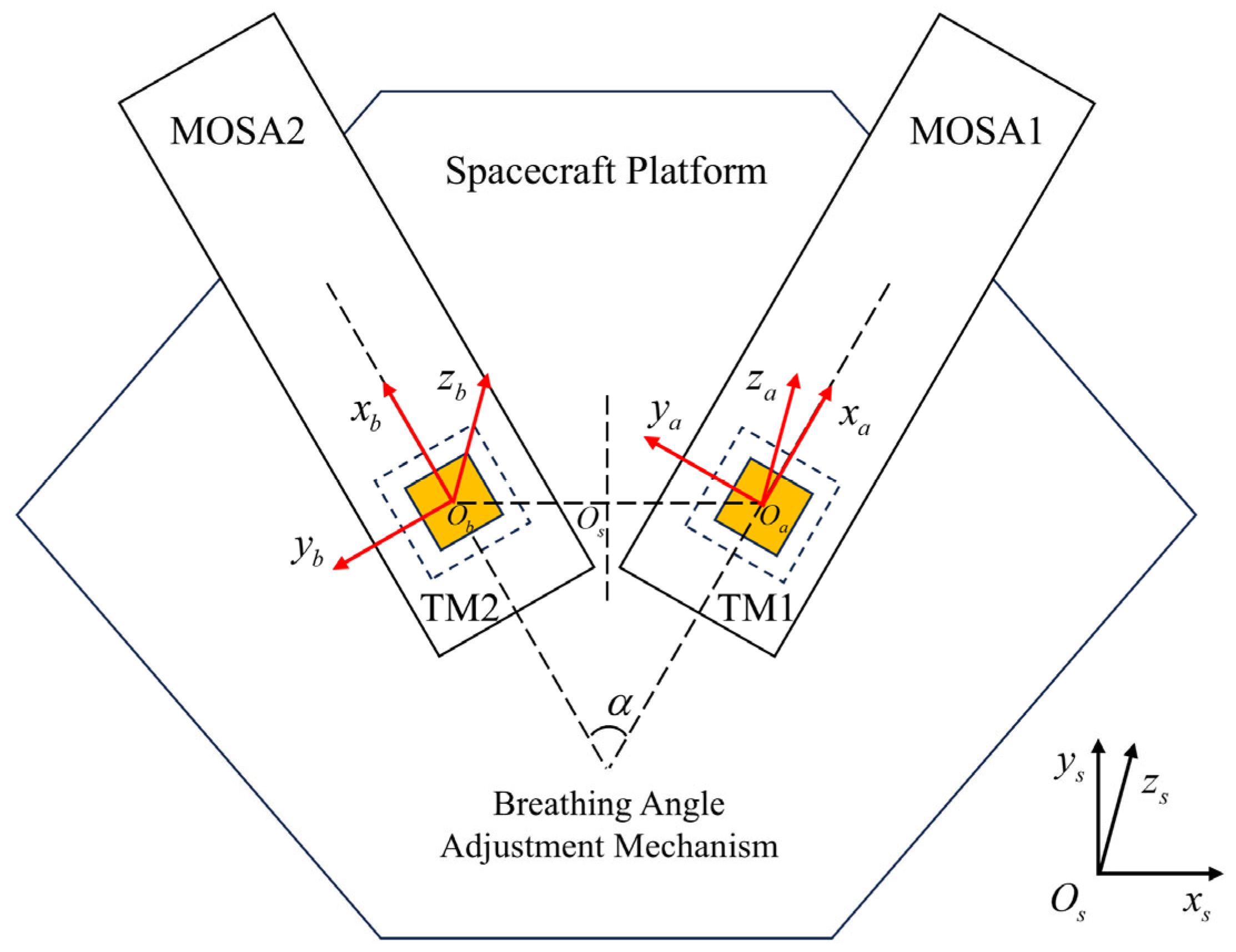
2.1. Coordinate System

The non-coaxial test mass layout of the space gravitational wave detection spacecraft is shown in Figure 1. The nominal position center of the test mass is assumed to be on the same line as the center of mass of the spacecraft. To facilitate the derivation and representation of the dynamics, the following right-handed coordinate system is defined:

• Spacecraft body coordinate system denoted as s: the origin of the coordinate system O_s is located at the center of mass of the spacecraft, y_s points outward along the axis of symmetry between the two interfering arms, and z_s points to the solar panel.
• TM1 coordinate system denoted as a: the origin of the coordinate system O_a is at the center of the nominal position of TM1, x_a is outward along the interfering arm, and z_a is pointing to the solar panel.
• TM2 coordinate system denoted as b: the origin of the coordinate system O_b is at the center of the nominal position of TM2, x_b is outward along the interfering arm, and z_b is pointing to the solar panel.

According to the basic principle of space gravitational wave detection, the x_a and x_b axes are sensitive axes and need to be focused on. The forces and stiffnesses involved in the formulas in this paper are all the effects per unit mass without any special explanation. In order to avoid misunderstanding, the variables are superscripted as the corresponding coordinate system, and subscripted as the relevant notation. For example, $f_m^s=\left[f_{mx}^s,f_{my}^s,f_{mz}^s\right]$ represents the force $f_m$ expressed in the coordinate system s. $W_a^b$ is defined as the transformation matrix from coordinate system a to coordinate system b and $r_{ij}^c$ as the vector from the center of i to the center of j in the coordinate system c, ${\phi }_1=〈x_s,x_a〉$, ${\phi }_2=〈x_s,x_b〉$.

2.2. Dynamics for Stiffness Identification

TM1 and TM2 adopt a non-coaxial and V-shaped layout in the spacecraft. According to the relative displacement of the test mass, the relative dynamics between the test mass and the spacecraft are constructed as follows:

$$\left\{\begin{array}{l}{\ddot{\mathit{r}}}_1^a={\mathit{r}}_{01}^a\times {\dot{\mathit{\omega }}}_B^a+2{\dot{\mathit{r}}}_{01}^a\times {\mathit{\omega }}_B^a+{\mathit{\omega }}_B^a\times \left({\mathit{r}}_{01}^a\times {\mathit{\omega }}_B^a\right)+{\mathit{f}}_1^a-{\mathit{f}}_B^a\\ {\ddot{\mathit{r}}}_2^b={\mathit{r}}_{02}^b\times {\dot{\mathit{\omega }}}_B^b+2{\dot{\mathit{r}}}_{02}^b\times {\mathit{\omega }}_B^b+{\mathit{\omega }}_B^b\times \left({\mathit{r}}_{02}^b\times {\mathit{\omega }}_B^b\right)+{\mathit{f}}_2^b-{\mathit{f}}_B^b\end{array}\right.$$

(1)

where ${\mathit{r}}_1^a={\left[x_1,y_1,z_1\right]}^{\mathrm{T}}$ and ${\mathit{r}}_2^b={\left[x_2,y_2,z_2\right]}^{\mathrm{T}}$ denote the displacement vector of TM1 and TM2 with respect to the nominal position, respectively. ${\mathit{r}}_{01}^a$ and ${\mathit{r}}_{02}^a$ denote the position vector of the center of mass of spacecraft to the centers of TM1 and TM2, respectively. ${\mathit{\omega }}_B^a$, ${\mathit{\omega }}_B^b$, and ${\mathit{\omega }}_B^s$ denote the angular velocity of the spacecraft. ${\mathit{f}}_1^a$ and ${\mathit{f}}_2^b$ denote the forces acting on TM1 and TM2, respectively, including stiffness effects, electrostatic forces, and bias disturbances. ${\mathit{f}}_B^a$ and ${\mathit{f}}_B^b$ denote the disturbance forces acting on the body of the spacecraft, including solar pressure, thruster noise, etc.

In this paper, only the translational degrees of freedom of the test mass are studied, and the rotational degrees of freedom are not involved. At the same time, the main diagonal elements in the stiffness matrix play a major role, while the non-main diagonal elements, i.e., the stiffness cross-coupling terms, can be ignored due to the relatively small value. Then, the force acting on the test mass can be expressed as follows:

$$\left\{\begin{array}{l}{\mathit{f}}_1^a={\mathbf{\Omega }}_1{\mathit{r}}_1^a+{\mathit{f}}_{\mathrm{e}1}^a+{\mathit{f}}_{D1}^a\\ {\mathit{f}}_2^b={\mathbf{\Omega }}_2{\mathit{r}}_2^b+{\mathit{f}}_{e2}^b+{\mathit{f}}_{D2}^b\end{array}\right.$$

(2)

where ${\Omega }_1=diag\left(k_{1xx},k_{1yy},k_{1zz}\right)$ and ${\Omega }_2=diag\left(k_{2xx},k_{2yy},k_{2zz}\right)$ denote the simplified stiffness matrix of TM1 and TM2, respectively. ${\mathit{f}}_{e1}^a$ and ${\mathit{f}}_{e2}^b$ denote the electrostatic forces acting on TM1 and TM2, respectively. ${\mathit{f}}_{D1}^a$ and ${\mathit{f}}_{D2}^b$ denote the bias disturbance to which TM1 and TM2 are subjected, respectively. The bias disturbance refers to a constant or very slowly changing disturbance force in dynamics, such as the forces produced by bias effects in the physical field.

By converting Equation (1) to the TM1 coordinate system, the two equations make a difference to eliminate the spacecraft acceleration disturbance ${\mathit{f}}_B^a$, which can be obtained as follows:

$$\begin{array}{ll}{\mathit{W}}_b^a{\ddot{\mathit{r}}}_2^b-{\ddot{\mathit{r}}}_1^a& =\left({\mathit{r}}_{12}^a\times {\dot{\mathit{\omega }}}_B^a+2{\dot{\mathit{r}}}_{12}^a\times {\mathit{\omega }}_B^a+{\mathit{\omega }}_B^a\times \left({\mathit{r}}_{12}^a\times {\mathit{\omega }}_B^a\right)\right)+{\mathit{W}}_b^a{\mathit{f}}_2^b-{\mathit{f}}_1^a\\ & ={\mathit{W}}_s^a\left({\mathit{r}}_{12}^s\times {\dot{\mathit{\omega }}}_B^s+2{\dot{\mathit{r}}}_{12}^s\times {\mathit{\omega }}_B^s+{\mathit{\omega }}_B^s\times \left({\mathit{r}}_{12}^s\times {\mathit{\omega }}_B^s\right)\right)+{\mathit{W}}_b^a{\mathit{f}}_2^b-{\mathit{f}}_1^a\end{array}$$

(3)

Similarly, by converting Equation (1) to the TM2 coordinate system, the two equations make a difference to eliminate the spacecraft acceleration disturbance ${\mathit{f}}_B^b$, which can be obtained as follows:

$$\begin{array}{ll}{\mathit{W}}_a^b{\ddot{\mathit{r}}}_1^a-{\ddot{\mathit{r}}}_2^b& =-\left({\mathit{r}}_{12}^b\times {\dot{\mathit{\omega }}}_B^b+2{\dot{\mathit{r}}}_{12}^b\times {\mathit{\omega }}_B^b+{\mathit{\omega }}_B^b\times \left({\mathit{r}}_{12}^b\times {\mathit{\omega }}_B^b\right)\right)+{\mathit{W}}_a^b{\mathit{f}}_1^a-{\mathit{f}}_2^b\\ & =-{\mathit{W}}_s^b\left({\mathit{r}}_{12}^s\times {\dot{\mathit{\omega }}}_B^s+2{\dot{\mathit{r}}}_{12}^s\times {\mathit{\omega }}_B^s+{\mathit{\omega }}_B^s\times \left({\mathit{r}}_{12}^s\times {\mathit{\omega }}_B^s\right)\right)+{\mathit{W}}_a^b{\mathit{f}}_1^a-{\mathit{f}}_2^b\end{array}$$

(4)

where ${\mathit{r}}_{12}^s={\mathit{r}}_{02}^s-{\mathit{r}}_{01}^s$ denotes the position vector from the center of TM1 to the center of TM2. The coordinate transformation matrix can be specifically expressed as follows:

$${\mathit{W}}_a^b={\left({\mathit{W}}_b^a\right)}^{-1}=\left[\begin{array}{ccc}\cos \alpha & \sin \alpha & 0\\ -\sin \alpha & \cos \alpha & 0\\ 0& 0& 1\end{array}\right]$$

(5)

$${\mathit{W}}_s^a=\left[\begin{array}{ccc}\cos {\phi }_1& \sin {\phi }_1& 0\\ -\sin {\phi }_1& \cos {\phi }_1& 0\\ 0& 0& 1\end{array}\right]$$

(6)

$${\mathit{W}}_s^b=\left[\begin{array}{ccc}\cos {\phi }_2& \sin {\phi }_2& 0\\ -\sin {\phi }_2& \cos {\phi }_2& 0\\ 0& 0& 1\end{array}\right]$$

(7)

Since the distance between the test masses is much larger than their motion, it is known that $r_{12x}^s$ is much larger than $r_{12y}^s$ and $r_{12z}^s$. Taking the respective sensitive axis components of Equations (3) and (4), and eliminating the major angular acceleration disturbance associated with $r_{12x}^s$, the following equation can be obtained:

$$\begin{array}{c}\sin {\phi }_1\left({\ddot{x}}_1\cos \alpha +{\ddot{y}}_1\sin \alpha -{\ddot{x}}_2\right)+\sin {\phi }_2\left({\ddot{x}}_2\cos \alpha -{\ddot{y}}_2\sin \alpha -{\ddot{x}}_1\right)\\ +\sin \left({\phi }_1-{\phi }_2\right){\left({\mathit{r}}_{12}^s\times {\dot{\mathit{\omega }}}_B^s+2{\dot{\mathit{r}}}_{12}^s\times {\mathit{\omega }}_B^s+{\mathit{\omega }}_B^s\times \left({\mathit{r}}_{12}^s\times {\mathit{\omega }}_B^s\right)\right)}_{x_s}\\ =\sin {\phi }_1\left(\left(k_{1xx}{x}_1+f_{e1x}^a+f_{D1x}^a\right)\cos \alpha +\left(k_{1yy}{y}_1+f_{e1y}^a+f_{D1y}^a\right)\sin \alpha -k_{2xx}{x}_2-f_{e2x}^b-f_{D2x}^b\right)\\ +\sin {\phi }_2\left(\left(k_{2xx}{x}_2+f_{e2x}^b+f_{D2x}^b\right)\cos \alpha -\left(k_{2yy}{y}_2+f_{e2y}^b+f_{D2y}^b\right)\sin \alpha -k_{1xx}{x}_1-f_{e1x}^a-f_{D1x}^a\right)\end{array}$$

(8)

Since the excitation signal of the spacecraft body is not applied during the identification process in this paper, the components of the angular velocity and angular acceleration related terms on the x_s axis, i.e., ${\left({\mathit{r}}_{12}^s\times {\dot{\mathit{\omega }}}_B^s+2{\dot{\mathit{r}}}_{12}^s\times {\mathit{\omega }}_B^s+{\mathit{\omega }}_B^s\times \left({\mathit{r}}_{12}^s\times {\mathit{\omega }}_B^s\right)\right)}_{x_s}$, are negligible, with small values. Equation (8) is written in the form of a matrix, which can be expressed as follows:

$${\left[\begin{array}{c}\sin {\phi }_1\cos \alpha -\sin {\phi }_2\\ \sin {\phi }_2\cos \alpha -\sin {\phi }_1\\ \sin {\phi }_1\sin \alpha \\ -\sin {\phi }_2\sin \alpha \end{array}\right]}^T\left(\left[\begin{array}{c}{k}_{1xx}{x}_1\\ k_{2xx}{x}_2\\ k_{1yy}{y}_1\\ k_{2yy}{y}_2\end{array}\right]+\left[\begin{array}{c}{f}_{e1x}^a\\ f_{e2x}^b\\ f_{e1y}^a\\ f_{e2y}^b\end{array}\right]+\left[\begin{array}{c}{f}_{D1x}^a\\ f_{D2x}^b\\ f_{D1y}^a\\ f_{D2y}^b\end{array}\right]-\left[\begin{array}{c}{\ddot{x}}_1\\ {\ddot{x}}_2\\ {\ddot{y}}_1\\ {\ddot{y}}_2\end{array}\right]\right)=0$$

(9)

The above formula combines the dynamics and the decomposition of non-coaxial double sensitive axes, effectively stripping off the influences of the spacecraft acceleration disturbance and the main angular acceleration disturbance on on-orbit identification. The dynamics of the test mass for stiffness identification have been derived in the non-coaxial case, which provides a theoretical basis for the subsequent parameter identification.

2.3. On-Orbit Stiffness Identification Method

According to the above dynamics derivation, it can be noted that the stiffness and bias disturbance combination term in Equation (9) are both linear parameter identifications. By separating the parameters to be identified and the measured, Equation (9) is further written as follows:

$$\mathit{{\rm K}}\left(\left[\begin{array}{c}{\ddot{x}}_1\\ {\ddot{x}}_2\\ {\ddot{y}}_1\\ {\ddot{y}}_2\end{array}\right]-\left[\begin{array}{c}{f}_{e1x}^a\\ f_{e2x}^b\\ f_{e1y}^a\\ f_{e2y}^b\end{array}\right]\right)=\left[\begin{array}{cc}\mathit{{\rm K}}\mathit{\Lambda }& 1\end{array}\right]\left[\begin{array}{c}{k}_{1xx}\\ k_{2xx}\\ k_{1yy}\\ k_{2yy}\\ R\end{array}\right]$$

(10)

where $\mathit{{\rm K}}$ and $\mathit{\Lambda }$ denote the coefficient matrix. $R$ denotes the bias disturbance combination term. It is expressed as follows:

$$\mathit{{\rm K}}={\left[\begin{array}{c}\sin {\phi }_1\cos \alpha -\sin {\phi }_2\\ \sin {\phi }_2\cos \alpha -\sin {\phi }_1\\ \sin {\phi }_1\sin \alpha \\ -\sin {\phi }_2\sin \alpha \end{array}\right]}^T$$

(11)

$$\mathit{\Lambda }=diag\left(x_1,x_2,y_1,y_2\right)$$

(12)

$$\mathrm{R}=\mathit{{\rm K}}{\left[f_{D1x}^a,f_{D2x}^b,f_{D1y}^a,f_{D2y}^b\right]}^{\mathrm{T}}$$

(13)

Then, Equation (10) can be equated to:

$$\mathit{y}={\mathit{\psi }}^{\mathrm{T}}\mathit{\theta }$$

(14)

where y denotes the output matrix, ψ^T denotes the weight matrix, and θ denotes the parameter to be identified, including the stiffness and bias disturbance combination term. It is worth noting that we focus on stiffness identification of the test mass sensitive axis, while non-sensitive axis stiffness and bias disturbance combination term identification are not within the scope of this paper.

While linear parameter identification algorithms are well-established, practical implementation in space missions must account for constraints such as periodic calibration windows, limited onboard computing resources, and satellite–ground data transmission bottlenecks. To address these challenges, this paper adopts a recursive least squares (RLS) algorithm for online parameter identification. The basic principle is to minimize the residual sum of squares and adjust the weights of old and new data through the forgetting factor. The specific algorithm update formula is as follows:

$$\left\{\begin{array}{l}{\mathit{K}}_n={\displaystyle \frac{{\mathit{P}}_{n-1}{\mathit{\psi }}_n}{\lambda +{\mathit{\psi }}_n^{\mathrm{T}}{\mathit{P}}_{n-1}{\mathit{\psi }}_n}}\\ {\widehat{\mathit{\theta }}}_n={\widehat{\mathit{\theta }}}_{n-1}+{\mathit{K}}_n\left({\mathit{y}}_n-{\mathit{\psi }}^{\mathrm{T}}{\widehat{\mathit{\theta }}}_n\right)\\ {\mathit{P}}_n={\displaystyle \frac{1}{\lambda }}\left(\mathit{I}-{\mathit{K}}_n{\mathit{\psi }}_n^{\mathrm{T}}\right){\mathit{P}}_{n-1}\end{array}\right.$$

(15)

where ${\widehat{\mathit{\theta }}}_n$ denotes the recursive parameter to be identified, and λ denotes the forgetting factor. K_n and P_n denote the gain matrix and the covariance matrix, respectively. The subscripts are the sampling points (n = 1, 2, …, N).

3. Methods for Enhancing Performance of Stiffness Identification

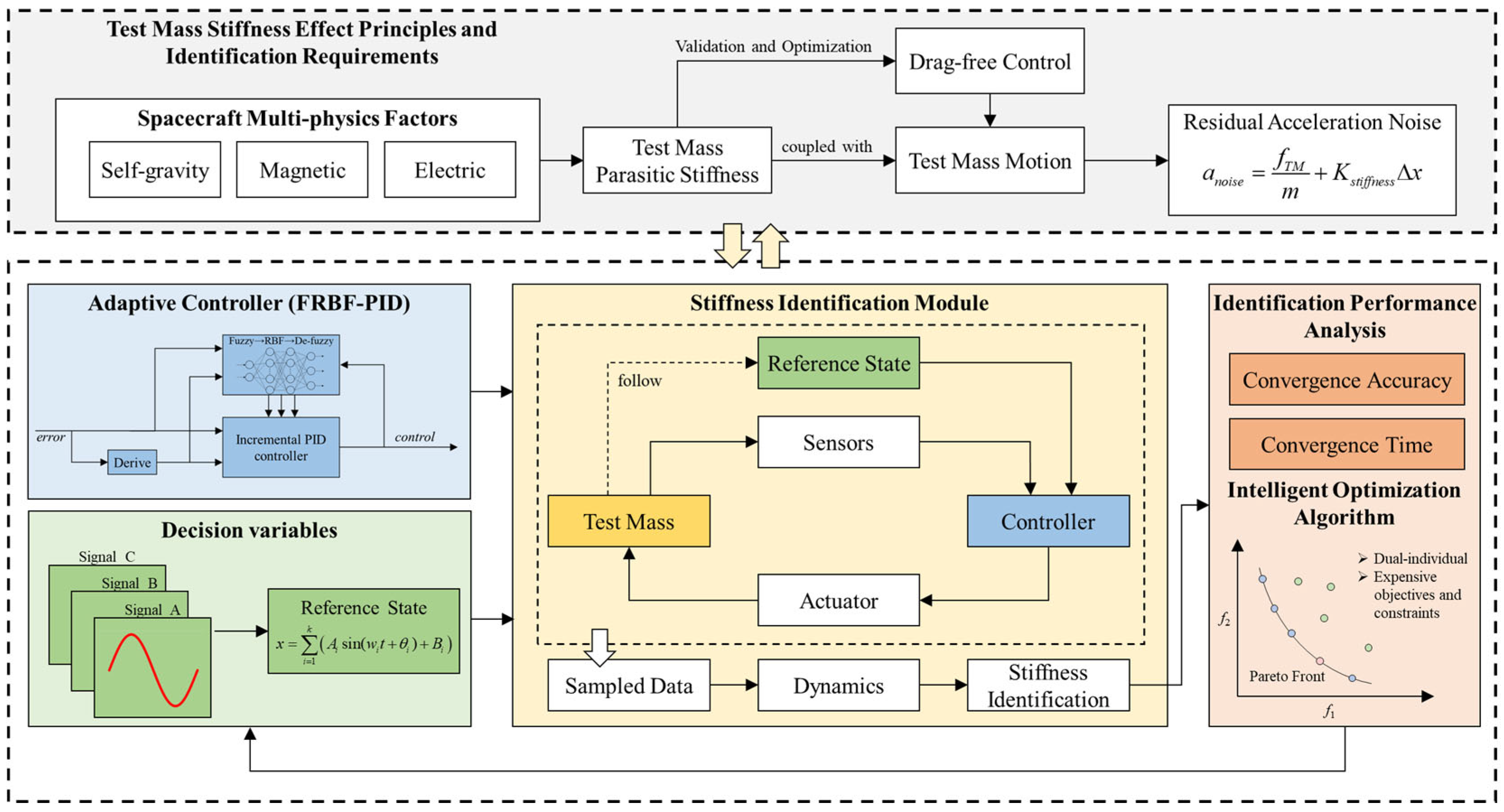
3.1. Research Framework

Figure 2 shows the overall research framework of this paper. The test mass stiffness caused by the spacecraft’s multiple physical factors is coupled with the test mass motion under drag-free control, thus generating part of residual acceleration noise. The identified stiffness can verify and optimize the control effect, further meeting noise suppression requirements during the mission period. The basic principles of test mass stiffness identification are presented in Section 2. By analyzing the dynamics, it can be noted that the necessary condition for stiffness identification is to control the relative displacement change between the test mass and the spacecraft, for which the key is to apply an excitation signal to the test mass to change its motion state. In space gravitational wave detection spacecraft, the signal excitation is applied by the electrostatic actuator. At the same time, the closed-loop control loop is applied to make the test mass follow the reference state. Utilizing onboard high-precision sensors and control loops [32,33], the test mass displacement, acceleration, applied electrostatic force, and other relevant data are sampled. Based on the derived dynamics of the test mass and the sampling data, test mass stiffness identification is realized by the parameter identification algorithm. The specific identification performances, including convergence time and accuracy, are calculated and analyzed. The motion state of the test mass, such as displacement and acceleration, has a direct impact on stiffness identification performance. To effectively enhance the performance, the reference state that is followed by the test mass under the action of the controller is optimized through the intelligent optimization algorithm so as to realize optimization of the test mass motion state. At the same time, the adaptive controller is introduced to meet the control requirements of different motion states. The specific methods for optimization and the adaptive controller involved in the process will be introduced in the following.

3.2. Motion State Optimization

3.2.1. Problem Definition

This paper carries out research related to the enhancement of stiffness identification performance, which requires finding the appropriate test mass motion state to optimally stimulate the system dynamics and meet identification requirements. Since the test mass follows the reference state under the action of the controller, this paper chooses to adjust the reference state so as to realize optimization of the motion state. To facilitate the optimization, the motion state of the test mass is parametrically characterized by a multi-frequency sinusoidal signal as follows:

$$x={\displaystyle \sum _{i=1}^k\left(A_i\sin (w_{i}t+{\theta }_i)+B_i\right)}$$

(16)

where A_i, ω_i, θ_i, and B_i denote the amplitude, frequency, phase, and bias of the signals, respectively, and k denotes the number of sub-signals or frequencies. The test mass is initially set at the center of the nominal position, i.e., the initial value of x is zero, which means the bias of the signal B_i = −A_isinθ_i. Thus, there are actually only A_i, ω_i, and θ_i as decision variables for the motion state in the optimization, which are denoted as X.

Considering the real-time and accuracy guarantees of parameter identification, convergence time and convergence accuracy are defined as the objective functions, which are calculated as follows:

$$ob{j}_1\left(\mathit{X},idx\right)=\min \left\{t:\left|{\widehat{\mathit{\theta }}}_n\left(idx\right)-{\widehat{\mathit{\theta }}}_{n-1}\left(idx\right)\right|\le \epsilon ,\forall n\ge t\right\}$$

(17)

$$ob{j}_2\left(\mathit{X},idx\right)=\sqrt{{\displaystyle \frac{1}{T-T_0}}{\displaystyle \sum _{n=T_0}^T{\left({\widehat{\mathit{\theta }}}_n\left(idx\right)-{\mathit{\theta }}_n\left(idx\right)\right)}^2}}$$

(18)

where obj₁ denotes the convergence time, expressing the minimum sampling time for which the identified parameter change continues to be less than a threshold ε. obj₂ denotes the convergence accuracy, expressed by calculating the RMSE after convergence. t, T₀, and T denote the sampling time, the convergence time, and the total sampling time, respectively. The subscripts n denotes the sampling points, and idx denotes the sequential number corresponding to the identified parameter.

Regarding the constraints, the maximum actuation output of the electrostatic force is limited in order to ensure the accuracy of the electrostatic force control and prevent the risk of large electrostatic force. Correspondingly, the motion state of the test mass should also satisfy the constraints to ensure the effectiveness of the control. In addition, a safe distance between the test mass and the electrode cage should also be considered.

Then, we can describe the optimization problem as follows:

$$\left\{\begin{array}{c}find \mathit{X}=\left\{A_i,w_i,{\theta }_i\right\}\\ \min \left\{ob{j}_1\left(\mathit{X}\right),ob{j}_2\left(\mathit{X}\right)\right\}\\ s.t. {\displaystyle \sum _{i=1}^k{A}_i{w}_i^2}<{\alpha }_1{F}_{max},x_{max}<{\alpha }_{2}D\end{array}\right.$$

(19)

where F_max denotes the maximum actuated electrostatic force. D denotes the distance between the test mass and the electrode cage (4 mm on the sensitive axis for LPF [34]). α₁ and α₂ denote the adjustment factors to provide safety margins for the other factors.

It can be noted that the dynamics of the test mass for stiffness identification involve the motion states of TM1 and TM2 at the same time. According to the different configurations of the decision variables and the objective function, there exist different optimization schemes to choose from. For example, when optimizing the motion states of TM1 and TM2 to enhance the stiffness identification performance of the TM1 sensitive axis, it will be a dual-objective optimization with 2 × 3 × k decision variables. Analyzing and comparing the optimization effects of different configurations, as well as finding the most suitable one, are also part of the research in this paper.

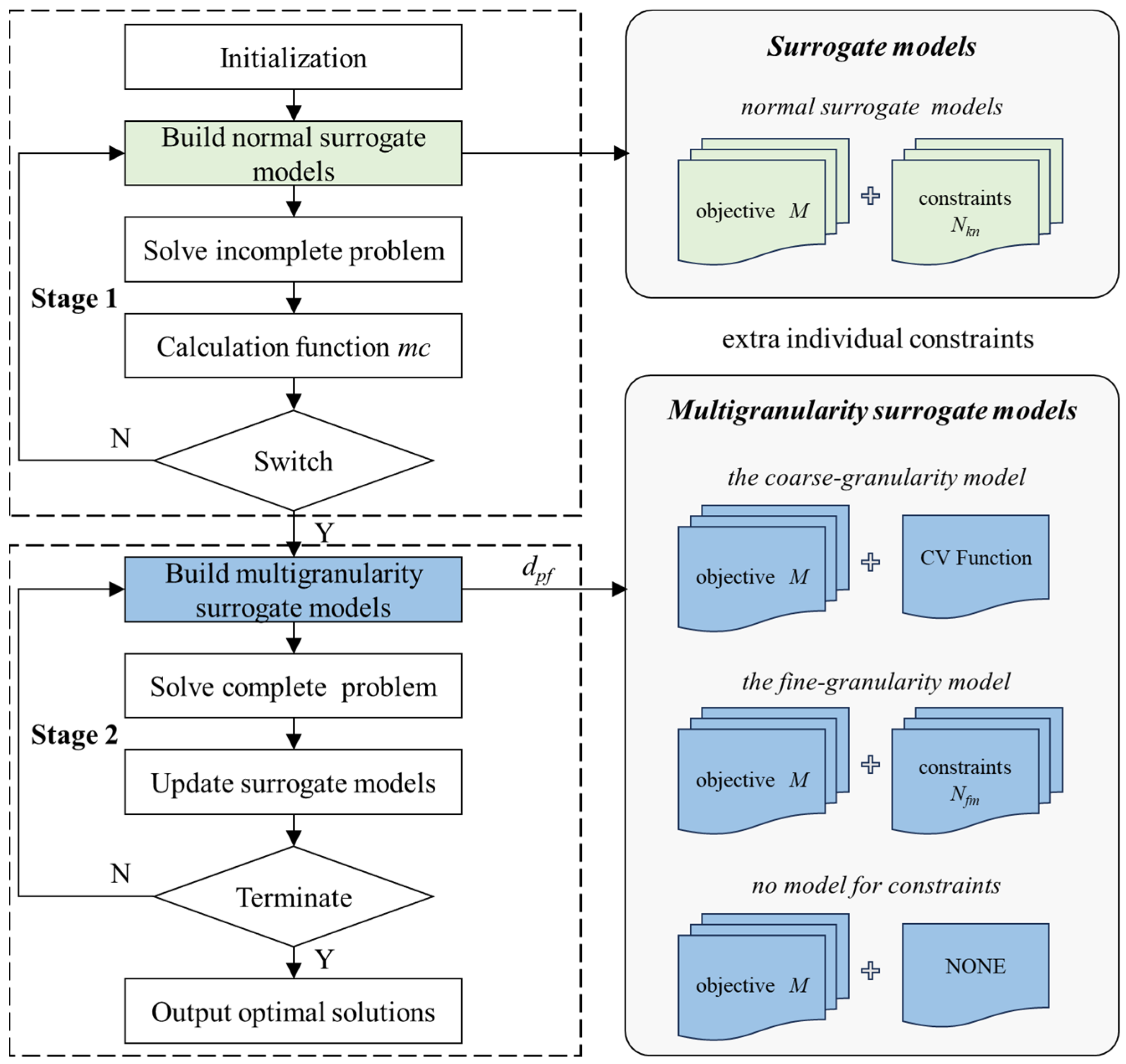
3.2.2. Optimization Algorithm

A large number of intelligent optimization algorithms have been proposed to solve optimization problems with different characteristics. The stiffness identification studied in this paper involves a dynamic model, noise disturbance, time series simulation, etc., which are computationally expensive. Meanwhile, the corresponding objectives and constraints are proposed around TM1 and TM2, and there exists a certain influence as well as a primary and secondary relationship between them.

Zhang Y J et al. [35] developed a multigranularity surrogate-assisted constrained evolutionary algorithm (MGSAEA) to address multi-objective optimization problems with expensive objectives and constraints. The algorithm achieves excellent performance on many test problems. In response to the characteristics of dual-individual, expensive objectives and constraints in the optimization problem of this paper, we improve on MGSAEA by considering individual progressive constraints and propose MGSAEA-IPC. Figure 3 shows the specific implementation of MGSAEA-IPC.

The first stage of the algorithm only considers the key individual constraints, and the second stage solves the complete optimization problem based on the multigranularity surrogate models. The selection of constraints is divided into individuals according to different test masses, and the constraints of the test mass for which stiffness needs to be identified are prioritized.

First, the population and archive are initialized to store possible solutions. The problem that only considers key individual constraints is solved in the first stage based on the normal surrogate models. The decision to switch to the next stage is made by computing the stage switching function. The maximum change rate mc of the ideal point in the past gap generation is chosen as the stage switching function and is calculated as follows:

$$mc=\underset{i=1,...,N}{\max }\left\{{\displaystyle \frac{\left|ob{j}_i^{iter}-ob{j}_i^{iter-gap}\right|}{\max \left\{\left|ob{j}_i^{iter-gap}\right|,\sigma \right\}}}\right\}$$

(20)

where $ob{j}_i^{iter}$ denotes the i-th value of the N objects for the ideal points at the iter-th generation population, and $\sigma$ denotes a small positive number to ensure that the denominator is not zero.

The second stage of optimization is entered when mc is less than a given threshold. Multigranularity surrogate models are constructed based on the distance from the population to the feasible region to solve the complete optimization problem. The idea is to balance the approximation accuracy and training cost of the surrogate models when solving multi-objective optimization problems with expensive objectives and constraints. In detail, when the population is far away from the feasible region, the surrogate models should enhance the exploration of the search space, and a coarse-granularity model, including objective functions and a constraint violation (CV) function, is sufficient. When the population is at the boundary of the feasible region, except the objective function, it is also necessary to take into account every constraint that is not fully satisfied, also called the construction of a fine-granularity model. When the population is within the feasible region, there is no need to construct any additional models for constraints, only to consider objective functions. The corresponding management strategies are also different for surrogate models with different granularities. The coarse-granularity model selects the solutions that survive to the next generation according to the constraint dominance principle (CDP), while the fine-granularity model assigns the same priority to objective optimization and constraint satisfaction through a multi-objective optimization approach.

The complete problem is solved optimally using the constructed multigranularity surrogate models and the training data are updated to reconstruct the relevant model. Until the abort condition is satisfied, the optimal solution from the archive is output as the result. Solving a multi-objective optimization problem using MGSAEA-IPC ultimately results in a Pareto front rather than a single solution [36], so the following strategy in Equation (21) is set up to select the optimal solution from the Pareto front. The minimum value of each objective during the optimization process is recorded as the optimal solution and it is used as the basis to normalize the values of all points in the Pareto front. According to the distance from all points to the unit point, the optimal solution can be determined based on the nearest distance principle:

$$x_{best}=\arg \underset{x}{\min }\sqrt{{\displaystyle \sum _{i=1,...,N}{\left(\frac{ob{j}_i-ob{j}_i^{min}}{ob{j}_i^{min}}\right)}^2}}$$

(21)

MGSAEA-IPC only considers a single individual constraint in the early stage of the search, i.e., stage one, which reduces the constraint complexity and lowers the computational cost. It also ensures the feasibility of the optimized solution under key individual constraints and helps to accelerate convergence and promote population diversity. Additionally, generating multigranularity surrogate models based on the position of the population in stage two prevents the population from falling into local optimum. Overall, the algorithm can effectively solve the optimization problem of stiffness identification performance in this paper.

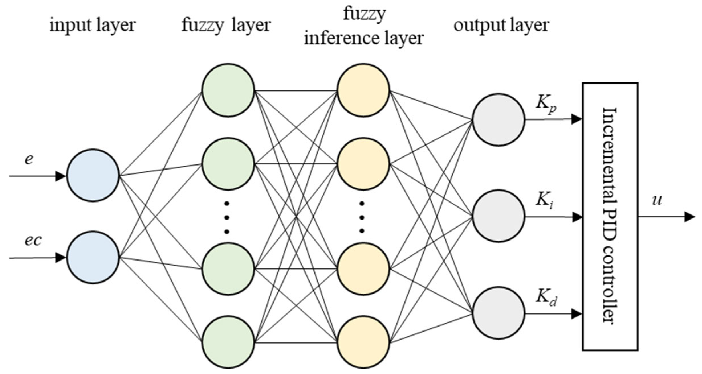
3.3. FRBF-PID Controller

In the process of optimizing the performance of stiffness identification, the motion states of the test mass are constantly changing due to the change of reference state. For the traditional PID controller, it is often difficult to achieve effective control in the face of complex and variational signals since its parameters are designed according to fixed rules. This results in the test mass not being able to effectively follow the reference state, while simultaneously introducing parameter uncertainty in the optimization process. Therefore, the design of a control strategy that can be adjusted in real time and adapted to different motion states is the key to the enhancement of stiffness identification performance. In this paper, a FRBF-PID controller is designed to realize adaptive control in the optimization process. Since the controller combines fuzzy logic, an RBF neural network, and PID control, it has a powerful adaptive ability, nonlinear modeling ability, and real-time learning and adjustment ability [37,38].

The FRBF-PID controller structure is shown in Figure 4. The inputs of the controller are the displacement error e and the error change rate ec, which are processed by the fuzzy RBF neural network. The results of the output layer are used to adjust the incremental PID controller in real time and then execute control.

The fuzzy RBF neural network includes an input layer, a fuzzy layer, a fuzzy inference layer, and an output layer. The relevant calculation formula is as follows.

(1) Input layer: Input data are passed directly to the next layer without processing.

$$f_1\left(i\right)=x_i$$

(22)

where i = 1, …, N.

(2) Fuzzy layer: A Gaussian basis function is selected as an affiliation function to fuzzy the data.

$$f_2\left(i,j\right)=\exp \left(-{\displaystyle \frac{{\left(f_1\left(i\right)-c_{ij}\right)}^2}{b_{ij}}}\right)$$

(23)

where j = 1, 2, …, M. c_ij and b_ij denote the center parameter and width parameter of the affiliation function, respectively.

(3) Fuzzy inference layer: Fuzzy rule matching is performed, where each neuron is equivalent to a fuzzy rule. The product is used instead of the operation of taking the smaller one.

$$f_3\left(l\right)=f_3\left(i,j\right)=f_2\left(1,i\right)\cdot f_2\left(2,j\right)$$

(24)

where l = 1, 2, …, M^N.

(4) Output layer: De-fuzzying is performed to obtain the rectified incremental PID controller parameters K_p, K_i, and K_d.

$$f_4\left(m\right)={\displaystyle \sum _l{f}_3\left(l\right)\cdot {\omega }_{net}\left(m,l\right)}$$

(25)

where m = 1, 2, 3. ω_net is the connection weight between the fuzzy inference layer and the output layer.

The performance metric function of the FRBF-PID controller is considered as follows:

$$E\left(n\right)={\displaystyle \frac{1}{2}}e{\left(n\right)}^2={\displaystyle \frac{1}{2}}{\left(r\left(n\right)-y\left(n\right)\right)}^2$$

(26)

where r(n) and y(n) denote the ideal and actual outputs at moment n, respectively.

Then, E(n) is minimized according to the principle of gradient descent, and the formula is updated for the relevant parameters of the network as follows:

$$\left\{\begin{array}{c}{\omega }_{ij}\left(n\right)={\omega }_{ij}\left(n-1\right)-{\eta }_{net}{\displaystyle \frac{\partial E}{\partial {\omega }_{ij}}}+{\alpha }_{net}\left({\omega }_{ij}\left(n-1\right)-{\omega }_{ij}\left(n-2\right)\right)\\ c_{ij}\left(n\right)=c_{ij}\left(n-1\right)-{\eta }_{net}{\displaystyle \frac{\partial E}{\partial c_{ij}}}+{\alpha }_{net}\left(c_{ij}\left(n-1\right)-c_{ij}\left(n-2\right)\right)\\ b_{ij}\left(n\right)=b_{ij}\left(n-1\right)-{\eta }_{net}{\displaystyle \frac{\partial E}{\partial b_{ij}}}+{\alpha }_{net}\left(b_{ij}\left(n-1\right)-b_{ij}\left(n-2\right)\right)\end{array}\right.$$

(27)

where η_net and α_net denote the learning rate and the momentum factor, respectively.

In summary, the expression of FRBF-PID controller is as follows:

$$\begin{array}{rl}u\left(n\right)=& u\left(n-1\right)+\Delta u\left(n\right)\\ =& u\left(n-1\right)+K_p\left[e\left(n\right)-e\left(n-1\right)\right]+K_{i}e\left(n\right)+K_d\left[e\left(n\right)-2e\left(n-1\right)+e\left(n-2\right)\right]\\ =& u\left(n-1\right)+f_4\left(1\right)\left[e\left(n\right)-e\left(n-1\right)\right]+f_4\left(2\right)e\left(n\right)+f_4\left(3\right)\left[e\left(n\right)-2e\left(n-1\right)+e\left(n-2\right)\right]\end{array}$$

(28)

In addition, the maximum actuation output of electrostatic force is limited to ensure the precision of electrostatic control and prevent the risk of large electrostatic force. To avoid the integral saturation caused by the output limitations of the incremental PID controller, it is set that when the control output reaches the saturation value, the integral term is temporarily frozen to prevent further accumulation of errors.

4. Numerical Simulation Experiments

4.1. Basic Simulation Environments

In order to verify the effectiveness of the proposed methods in this paper, numerical simulation experiments are carried out through MATLAB/Simulink. The simulation setup of the gravitational wave detection spacecraft is located in the heliocentric orbit, lagging behind the Earth by about 20°, with the sun vector and the spacecraft sailing normal at an angle of 30°. The center of TM1, the TM2 nominal position, and the MOSA link constitute an equilateral triangle with a side length of 0.4 m. Combined with the basic principles of space gravitational wave detection, we focus on the stiffness identification of the test mass sensitive axis, i.e., k_1xx and k_2xx. Therefore, the test mass is set to move along the sensitive axis in the form of a multi-frequency sinusoidal signal under the action of the FRBF-PID controller. The non-sensitive axis does not have a high requirement, only to maintain the nominal position of the axis under the action of the traditional PID controller. The sampling frequency of the system is 10 Hz, and the total simulation time is 1200 s. In addition, the influences of the displacement measurement noise N_m1 of the sensitive axis, the displacement measurement noise N_m2 of the non-sensitive axis, the acceleration measurement noise N_acc, and the electrostatic execution noise N_ele on parameter identification are considered in the simulation. The types of noise are all zero-mean Gaussian white noise with a mean square error of δ. The specific simulation parameter settings are shown in

Table 1. Parameter true values and noise settings used in the simulation.

Parameters	Value
[k1xx, k1yy, k1zz] (s−2)	[1,1,1] × 10−7
[k2xx, k2yy, k2zz] (s−2)	[1,1,1] × 10−7
fD1 (m·s−2)	[1,1,1] × 10−10
fD2 (m·s−2)	[1,1,1] × 10−10
Nm1 (m)	δ = 1×10−11
Nm2 (m)	δ = 1 × 10−8
Nacc (m·s−2)	δ = 1 × 10−12
Nele (m·s−2)	δ = 1 × 10−12

.

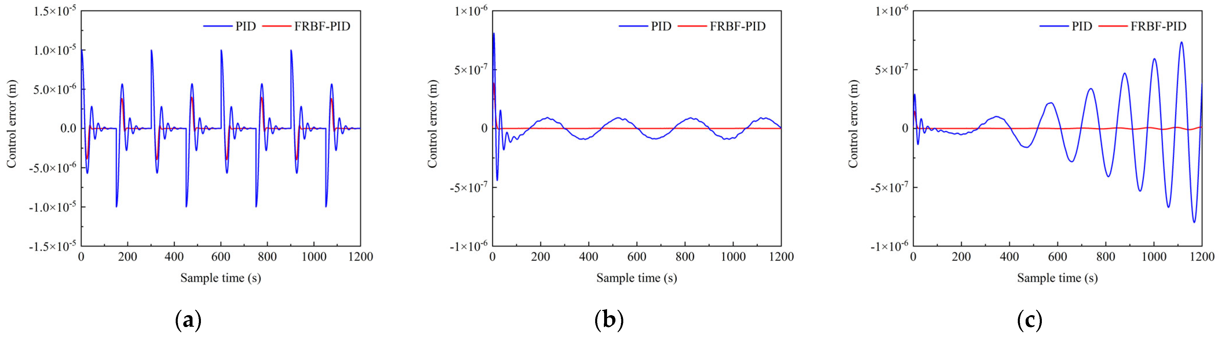
4.2. FRBF-PID Control Performance

In this paper, the FRBF-PID controller is designed to meet the control requirements of different motion states in the optimization. Set c_ij(0) = [−1, −0.5, −0.2, 0, 0.2, 0.5, 1], b_ij(0) = 0.2 × ones (2, 7), a learning rate η_net of 0.1, momentum factor α_net of 0.01, and adjusting the gain coefficients of the incremental PID as [0.5, 0.01, 10]. Three typical types of test signals, the pulse signal, the sinusoidal signal, and the swept signal (or chirp signal, a sinusoidal signal whose frequency changes over time) with an amplitude of 10⁻⁵ m, are chosen to be compared with the traditional PID controller. Figure 5 shows their control errors.

According to experimental results, the FRBF-PID controller can achieve effective control. For the pulse signal, the control effect is average but much more effective and converges faster than the PID controller. For the sinusoidal and swept signals, it is worth noting that the FRBF-PID controller shows sufficiently good performance. The signals can be effectively converged within 1 min and the steady-state error is less than 0.2% of the amplitude. As the frequency increases, the control oscillation is also smaller. Therefore, using the FRBF-PID controller designed in this paper can better control the test mass to follow different reference states in the form of multi-frequency sinusoidal signals, which can meet the control requirements involved in the subsequent optimization.

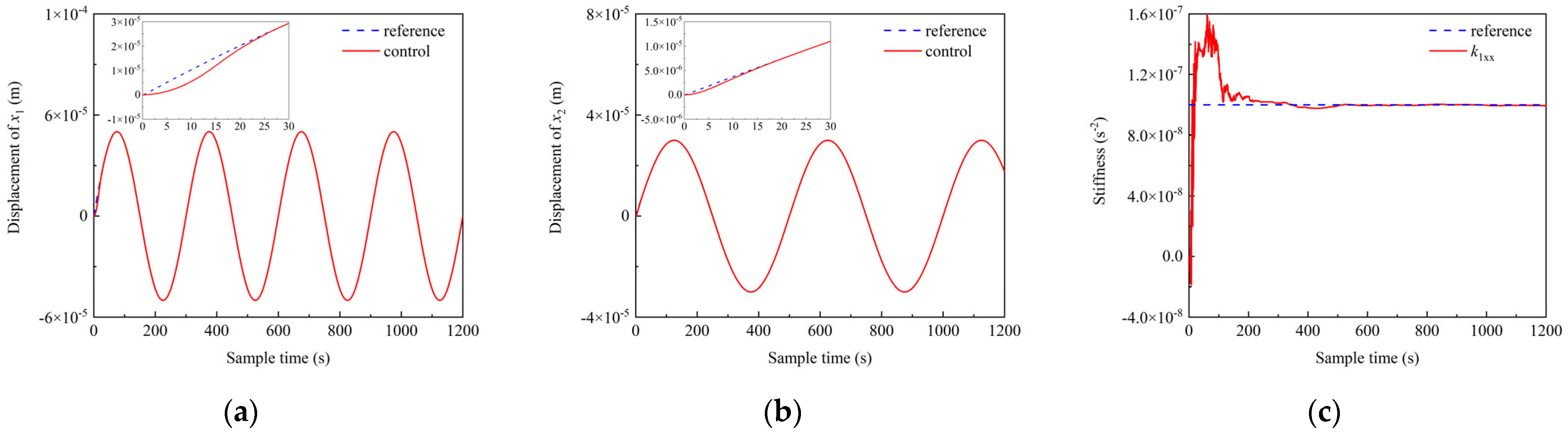
4.3. Stiffness Identification Performance

According to the truth value set in Table 1, the threshold ε corresponding to the convergence time of the parameter is set to 10⁻¹⁰ m/s². It means that only a change in the identification results consistently less than 0.1% of the truth value can be regarded as convergence. From the dynamics, we know that the motion states of TM1 and TM2 are coupled in stiffness identification. For this reason, the stiffness identification performance of the test mass sensitive axis under the different motion states of TM1 and TM2 is analyzed, taking TM1 as an example.

First, the performance of stiffness identification in the case of one fixed motion state is analyzed. Setting the reference state of TM1 and TM2, respectively, to x₁ = 5 × 10⁻⁵sin(2π/300·t) m and x₂ = 3 × 10⁻⁵sin(2π/500·t) m, the experimental results on stiffness identification are shown in Figure 6.

Under the action of the FRBF-PID controller, the motion state of the test mass can follow the reference state effectively within 2 min, the max error is less than 5 × 10⁻⁶ m, and the steady-error is less than 3 × 10⁻⁹ m. At the same time, k_1xx can be identified effectively in this motion state, with a convergence accuracy of 7.86 × 10⁻¹⁰ m/s² and a convergence time of 309.6 s.

Then, in the case of a single-frequency sinusoidal signal, the amplitude, frequency, and phase of the TM1 and TM2 reference states are changed simultaneously. The stiffness identification performance of TM1 under the corresponding motion state is shown in Figure 7. It can be seen that the choice of amplitude, frequency, and phase of the test mass does have a significant effect on the stiffness identification, but the relationship is not clearly enough due to the complexity and partial uncertainty of the identification model.

The trends in Figure 7 also show that the test mass stiffness identification performance is mainly affected by its own motion state. In generally, when the amplitude and frequency are larger, the stiffness identification performance is better. It is more obvious for the convergence time, which has a clear demarcation between right and left. By contrast, the convergence accuracy is affected a little bit more by the motion state of the other test mass. In addition, it is found that for the same motion state of TM1 and TM2, i.e., the main diagonal conditions, the convergence accuracy is much better than the nearby situation. For the phase, there is not an overall clear law, and the degree of influence compared to the magnitude and frequency is much smaller. Through the data distribution in the results, we can also clearly find that the convergence time and convergence accuracy are not completely positively correlated, and even in many cases they are contradictory. Therefore, it is difficult to unify the optimal, which is also in line with conventional knowledge. For this reason, this paper chooses multi-objective optimization instead of single-objective optimization through weighting or other ways. Finally, the experimental results also fully reflect that a single-frequency sinusoidal signal is not enough to effectively enhance the performance of stiffness identification. It is necessary to consider a more informative form of the motion state.

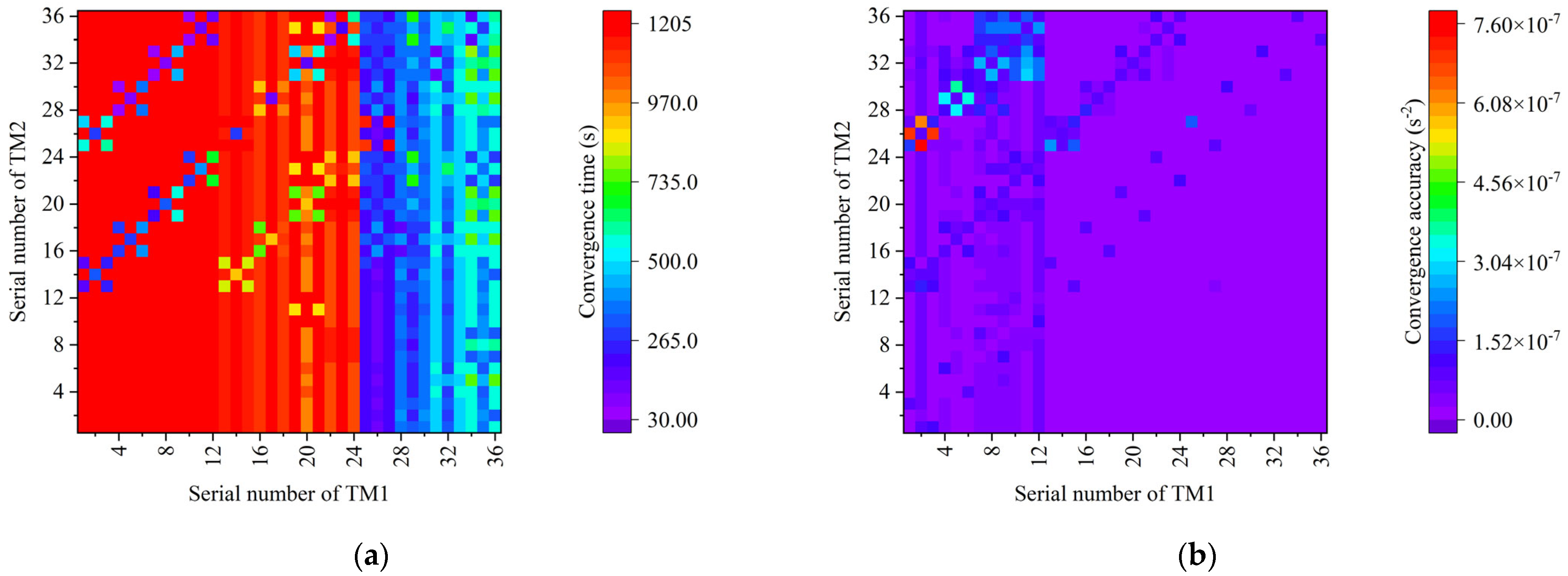
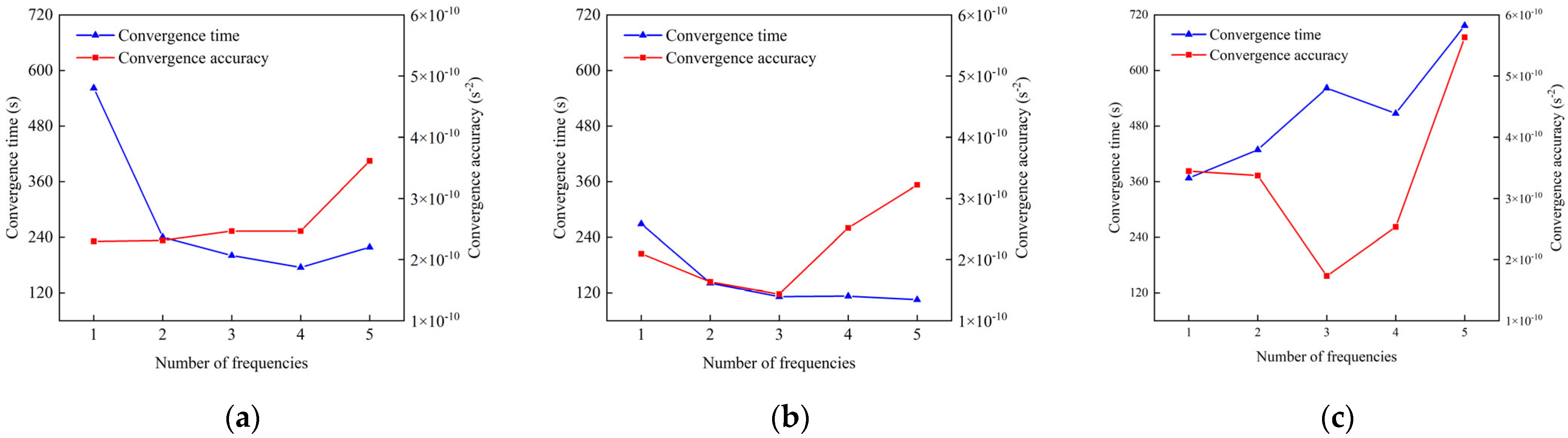
4.4. Stiffness Identification Performance Enhancement by Optimizing the Motion State

Combined with the analysis in Section 4.3, it can be seen that a single-frequency sinusoidal signal is not enough. For this reason, this paper chooses the motion state in the form of a multi-frequency sinusoidal signal to better stimulate the system response. Since both TM1 and TM2 motion states are involved in the dynamics for stiffness identification, there exist different optimization schemes to choose from based on different configurations of decision variables and objective functions. For the case of a single test mass, taking TM1 as an example, the specific configurations are shown in

Table 2. Different optimization configurations.

Scheme	Dec	Obj	Configuration
A	TM1	TM1	3 × k & 2
B	TM1 + TM2	TM1	2 × 3 × k & 2
C	TM1 + TM2	TM1 + TM2	2 × 3 × k & 4

Note: Take A with configuration of 3 × k & 2 as an example, 3 × k and 2 denote the dimensions of the decision variables and the objective functions, respectively. k denotes the number of frequencies of the multi-frequency sinusoidal signal.

. For example, scheme B represents that the motion state parameters of TM1 and TM2 are set as the decision variables, and the stiffness identification performance of the TM1 sensitive axis is set as the objective. In this case, the problem is a dual-objective constrained optimization problem with 18 decision variables.

Considering that the optimization problem in this paper has the characteristics of dual-individual, expensive objectives and constraints, MGSAEA-IPC is designed and used for optimization. The number of populations is set to 100, the number of iterations is set to 100, the gap of stage switching is set to 20, and the small positive number $\sigma$ is set to 10⁻³. The maximum electrostatic power output in the constraint is set to 10⁻⁷ m/s², the distance between the test mass sensitive axis and the electrode cage is set to 4 mm, and the corresponding adjusting factors are set to 0.5 and 0.1. In particular, for the case where there is only one test mass in scheme A, the constraint on the other test mass can be considered to be naturally satisfied and the algorithm still works. The experimental results of different optimization configurations are shown in Figure 8.

To express the optimized results more clearly, the convergence time and convergence accuracy are also weighted and transformed as M according to Equation (29):

$$M=weigh{t}_1\times ob{j}_1+weigh{t}_2\times ob{j}_2$$

(29)

where weight₁ and weight₂ are set to 1/60 and 10¹⁰, respectively.

The specific M of different optimization configurations is shown in Figure 9.

The experimental results show that there exist significant differences in the optimization performance corresponding to different schemes and different number of frequencies. This is mainly due to the different number of decision variables and objective functions under different configurations.

It is known that a single-frequency sinusoidal signal more easily satisfies the constraints, and thus is easier to control and optimize. But the information of this type of signal is limited, and the performance of stiffness identification is average. When the number of frequencies increases, the signal carries richer information, which is accompanied by a higher computational cost of optimization, as well as potentially better identification. However, due to the constraints of controller output, motion state, and other factors, the optimizable range of the multi-frequency sinusoidal signal is limited too. When the number of frequencies actually further increases, coupled with more decision variables, the optimization results gradually become less ideal. It is demonstrated to some degree by the trends in the curves of different schemes in Figure 8 and Figure 9, with schemes A and B being the most significant. For schemes A and B with the same number of objective functions, as the number of frequencies increases, more and more decision variables follow. The stiffness identification performance generally shows a trend of improving and then worsening, which can be reflected by the turning point in the curves. The number of frequencies corresponding to the turning point is also considered to be the optimal configuration under this scheme. However, for scheme C, the above analysis does not strictly follow. Scheme C has more decision variables and objective functions than schemes A and B, which directly leads to difficulties in reaching an optimization solution. The identification performance at different numbers of frequencies is generally poor compared to other schemes and worsens with a higher number of frequencies, as expected. The optimal number of frequencies for schemes A, B, and C are 4, 3, and 1, respectively. It is clear that the optimal result of scheme B is also the optimal result among all schemes, while scheme A is a little worse and scheme C is the worst.

The number of decision variables and objective functions in scheme B with the three-frequency sinusoidal signal is in the middle of all configurations. This allows the configuration to improve the quality of the solution to some extent by using more decision variables in the appropriate range. Correspondingly, the moderate complexity of the motion state is not difficult to control. At the same time, only considering the single test mass stiffness optimization performance also reduces the cost of the objective function calculation. In addition, it is worth noting that the stiffness parameters of both test masses can be viewed as constants and independent within a calibration cycle, and the identification scheme adopted in this paper is relatively inexpensive in terms of time and resource consumption. Therefore, although scheme B cannot optimize the stiffness identification performance on both test masses at the same time, it is perfectly acceptable to separately identify different test mass stiffnesses through this configuration, as long as we can obtain better parameter identification performance.

Further details about the optimization are described based on MGSAEA-IPC and the above optimal configuration, i.e., simultaneously optimizing the TM1 and TM2 motion states in the form of the three-frequency sinusoidal signal to enhance the stiffness identification performance of the TM1 sensitive axis. Figure 10 shows the optimized results under the optimal configuration.

The optimized motion state of the test mass satisfies the set constraints, as shown by the maximum displacement of TM1 and TM2 being less than 0.2 mm, and the designed FRBF-PID controller can realize effective control within 3 min. The max control error is less than 3 × 10⁻⁵ m and the steady-error is less than 5 × 10⁻⁹ m. In this motion state, the convergence time of test mass stiffness identification is 112.1 s, and the convergence accuracy is 1.44 × 10⁻¹⁰·s⁻², which is a significant optimization effect. It is also clearly reflected from the identification curve, for which convergence is faster and smoother.

In order to fully reflect the effectiveness of the proposed algorithm under this configuration, MGSAEA-IPC is compared with other multi-objective optimization algorithms, including typical multi-objective algorithms and some other novel algorithms for surrogate models. In additional, ablation experiments of MGSAEA-IPC are conducted, and the metric M of the different stringent convergence thresholds ε in the optimization results is also taken into account to better show the performance of the algorithm. All algorithms were evaluated under identical random seeds, ensuring fair comparison. The optimization results of different algorithms are shown in

Table 3. Optimization results of different algorithms.

Algorithm	Convergence Time (s)	Convergence Accuracy (s−2)	M (Default)	M (7 × 10−11)	M (5 × 10−11)	Final Accuracy (s−2)
NSGA-II [39]	141.0	1.44 × 10−10	3.79	9.73	10.82	5.86 × 10−11
NSGA-III [40]	125.9	2.40 × 10−10	4.50	7.39	7.39	3.60 × 10−12
C-MOEA/D [41]	76.2	1.13 × 10−09	12.55	8.83	9.52	5.90 × 10−11
C-TSEA [42]	218.8	2.44 × 10−10	6.08	13.53	13.64	9.10 × 10−12
SSDE [43]	177.1	3.34 × 10−10	6.30	6.11	6.23	2.02 × 10−10
CMOES [44]	175.1	1.61 × 10−10	4.53	6.75	6.75	1.25 × 10−10
MGSAEA [35]	103.7	4.68 × 10−10	6.41	8.99	8.99	1.90 × 10−10
MGSAEA*	191.9	2.31 × 10−10	5.51	11.36	11.53	5.50 × 10−11
MGSAEA-IPC	112.1	1.44 × 10−10	3.30	5.75	5.75	2.91 × 10−12

Note: MGSAEA* denotes MGSAEA-IPC without considering the priority of key individual constraints in stage one for ablation experiments. M(ε) denotes the metric M corresponding to the convergence threshold ε.

.

Compared with other algorithms, MGSAEA-IPC proposed in this paper performs well enough in the optimization problem of stiffness identification performance enhancement under the given optimal configuration. It achieves the best balance between convergence time and convergence accuracy, and the default M reached the best value of 3.30. When the convergence threshold is made stricter, the algorithm still performs the best, which demonstrates its stable convergence and good performance. At the same time, the final identification accuracy is less than 3 × 10⁻¹² s⁻², which is also the best among all algorithms. In addition, ablation experiments with MGSAEA and MGSAEA* also fully demonstrate that the improvements to individual progressive constraints are extremely meaningful and effective, nearly doubling the performance improvement.

Finally, in order to verify the general validity of the optimized motion state in this paper, the truth value of the stiffness of the test mass on the sensitive axis was changed. The identification curves are shown in Figure 11. The results show that for different truth values of stiffness, the optimized test mass motion state can always achieve better identification performance. The optimized motion state can fully stimulate the dynamic system response rather than the optimization of a random or single specific case.

5. Conclusions

In this study, we optimize the motion state of a test mass to enhance stiffness identification performance, and the experimental results demonstrate that our proposed method is significant, including faster convergence times and higher convergence accuracy. Through the above work, we can draw the following conclusions, specifically:

(1) Based on the constructed dynamics of a test mass for stiffness identification, the recursive least squares algorithm can realize the stiffness identification of the test mass sensitive axis within 20 min, but the specific identification performance is affected by the motion state of the test mass, and there are not obvious laws.

(2) The designed FRBF-PID controller can meet the complex control requirements of different motion states. It can realize effective control within 3 min, with a steady-state error of less than 5 × 10⁻⁹ m.

(3) Considering the balance between onboard resources and identification performance, the scheme of simultaneously optimizing TM1 and TM2 motion states in the form of a three-frequency sinusoidal signal to enhance the identification performance of single test mass stiffness is more appropriate and cost effective.

(4) The proposed MGSAEA-IPC has obvious advantages over other multi-objective optimization algorithms in solving this problem under the given optimal configuration, which can be well adapted to the characteristics of the stiffness optimization problem. The final optimized motion state can be applied to different stiffness configurations without violating the constraints. The convergence time of the final optimization is less than 2 min, and the convergence accuracy is less than 1.5 × 10⁻¹⁰ s⁻², which are clear improvements compared to before.

(5) The method designed in this paper integrates an online identification algorithm, advanced control strategy, and intelligent optimization algorithm. It can effectively enhance stiffness identification performance based on motion state optimization, which can provide ideas and design references for subsequent related identification and control.

References

1. Giammarchi, M.; Ricci, F. Gravitational Waves, Event Horizons and Black Hole Observation: A New Frontier in Fundamental Physics. Symmetry 2022, 14, 2276. [Google Scholar] [CrossRef]
2. Mastrogiovanni, S.; Karathanasis, C.; Gair, J.; Ashton, G.; Rinaldi, S.; Huang, H.Y.; Dálya, G. Cosmology with gravitational waves: A review. Ann. Phys. 2024, 536, 2200180. [Google Scholar] [CrossRef]
3. Wu, Y.L.; Hu, W.R.; Wang, J.Y.; Chang, J.; Cai, R.G.; Zhang, Y.H.; Luo, Z.R.; Lu, Y.J.; Zhou, Y.F.; Guo, Z.K. Review and scientific objectives of spaceborne gravitational wave detection missions. Chin. J. Space Sci. 2023, 43, 589–599. [Google Scholar] [CrossRef]
4. Bayle, J.B.; Bonga, B.; Caprini, C.; Doneva, D.; Muratore, M.; Petiteau, A.; Rossi, E.; Shao, L. Overview and progress on the Laser Interferometer Space Antenna mission. Nat. Astron. 2022, 6, 1334–1338. [Google Scholar] [CrossRef]
5. Luo, Z.R.; Wang, Y.; Wu, Y.L.; Hu, W.R.; Jin, G. The Taiji program: A concise overview. Prog. Theor. Exp. Phys. 2021, 2021, 05A108. [Google Scholar] [CrossRef]
6. Mei, J.; Bai, Y.Z.; Bao, J.; Barausse, E.; Cai, L.; Canuto, E.; Cao, B.; Chen, W.M.; Chen, Y.; Ding, Y.W.; et al. The TianQin project: Current progress on science and technology. Prog. Theor. Exp. Phys. 2021, 2021, 05A107. [Google Scholar] [CrossRef]
7. Armano, M.; Audley, H.; Baird, J.; Binetruy, P.; Born, M.; Bortoluzzi, D.; Castelli, E.; Cavalleri, A.; Cesarini, A.; Cruise, A.M.; et al. Beyond the required LISA free-fall performance: New LISA pathfinder results down to 20 μHz. Phys. Rev. Lett. 2018, 120, 061101. [Google Scholar] [CrossRef]
8. Luo, Z.R.; Zhang, M.; Wu, Y.L. Recent status of Taiji program in China. Chin. J. Space Sci. 2022, 42, 536–538. [Google Scholar] [CrossRef]
9. Luo, J.; Bai, Y.Z.; Cai, L.; Cao, B.; Chen, W.M.; Chen, Y.; Cheng, D.C.; Ding, Y.W.; Duan, H.Z.; Gou, X.; et al. The first round result from the Tianqin-1 satellite. Cl. Quantum Grav. 2020, 37, 185013. [Google Scholar] [CrossRef]
10. Jennrich, O. LISA technology and instrumentation. Cl. Quantum Grav. 2009, 26, 153001. [Google Scholar] [CrossRef]
11. Luo, Z.R.; Bai, S.; Bian, X.; Chen, G.; Dong, P.; Dong, Y. Space laser interferometry gravitational wave detection. Adv. Mech. 2013, 43, 415–447. [Google Scholar]
12. Wang, Z.Q.; Gao, D.; Deng, K.N.; Lu, Y.; Ma, S.D.; Zhao, J. Robot base position and spacecraft cabin angle optimization via homogeneous stiffness domain index with nonlinear stiffness characteristics. Robot. Comput. Integr. Manuf. 2024, 90, 102793. [Google Scholar] [CrossRef]
13. Piskarev, Y.; Sun, Y.; Righi, M.; Boehler, Q.; Chautems, C.; Fischer, C.; Nelson, B.J.; Shintake, J.; Floreano, D. Fast-Response Variable-Stiffness Magnetic Catheters for Minimally Invasive Surgery. Adv. Sci. 2024, 11, 2305537. [Google Scholar] [CrossRef]
14. Li, H.; Bi, K.M.; Hao, H.; Yu, Y.; Xu, L.H. Experimental study of a novel quasi-active negative stiffness damper system for achieving optimal active control performance. Eng. Struct. 2024, 299, 117082. [Google Scholar] [CrossRef]
15. Weber, W.J.; Bortoluzzi, D.; Cavalleri, A.; Carbone, L.; Lio, M.D.; Dolesi, R.; Fontana, G.; Hoyle, C.D.; Hueller, M.; Vitale, S. Position sensors for flight testing of LISA drag-free control. Gravitational-Wave Detect. 2003, 4856, 31–42. [Google Scholar]
16. Armanoa, M.; Audleyb, H.; Augerc, G.; Bairdn, J.; Binetruyc, P.; Bornb, M.; Bortoluzzid, D.; Brandte, N.; Bursit, A.; Calenof, M.; et al. Constraints on LISA Pathfinder’s self-gravity: Design requirements, estimates and testing procedures. Cl. Quantum Grav. 2016, 33, 235015. [Google Scholar] [CrossRef]
17. Gou, X.Y.; Wang, L.J.; Xu, X.M.; Zou, K.; Jiang, Q.H. Study on Dynamic Coordination Condition of Displacement Drag-free Control. J. Astron. 2024, 45, 540–549. [Google Scholar]
18. Jiao, B.H.; Liu, Q.F.; Dang, Z.H.; Yue, X.K.; Zhang, Y.H.; Xia, Y.Q.; Duan, L.; Hu, Q.L.; Yue, C.L.; Wang, P.C.; et al. A review on DFACS (I): System design and dynamics modeling. Chin. J. Aeronaut. 2024, 37, 92–119. [Google Scholar] [CrossRef]
19. Yue, C.L.; Jiao, B.H.; Dang, Z.H.; Yue, X.K.; Zhang, Y.H.; Xia, Y.Q.; Duan, L.; Hu, Q.L.; Liu, Q.F.; Wang, P.C.; et al. A review on DFACS (II): Modeling and analysis of disturbances and noises. Chin. J. Aeronaut. 2024, 37, 120–147. [Google Scholar] [CrossRef]
20. Ziegler, T.; Fichter, W. Test mass stiffness estimation for the LISA Pathfinder drag-free system. In Proceedings of the AIAA Guidance, Navigation and Control Conference and Exhibit, Hilton Head, SC, USA, 20 August–23 August 2007; Volume 6669. [Google Scholar]
21. Nofrarias, M.; Röver, C.; Hewitson, M.; Monsky, A.; Heinzel, G.; Danzmann, K.; Ferraioli, L.; Hueller, M.; Vitale, S. Bayesian parameter estimation in the second LISA Pathfinder mock data challenge. Phys. Rev. D 2010, 82, 122002. [Google Scholar] [CrossRef]
22. Congedo, G.; Ferraioli, L.; Hueller, M.; Marchi, F.D.; Vitale, S.; Armano, M.; Hewitson, M.; Nofrarias, M. Time domain maximum likelihood parameter estimation in LISA Pathfinder data analysis. Phys. Rev. D 2012, 85, 122004. [Google Scholar] [CrossRef]
23. Armano, M.; Audley, H.; Baird, J.; Binetruy, P.; Born, M.; Bortoluzzi, D.; Castelli, E.; Cavalleri, A.; Cesarini, A.; Cruise, A.M.; et al. Calibrating the system dynamics of LISA Pathfinder. Phys. Rev. D 2018, 97, 122002. [Google Scholar] [CrossRef]
24. Tang, N.B.; Yang, Z.G.; Cai, Z.M.; Fang, Z.R.; Liu, Y.; Hu, H.Y.; Li, H.W. Identification of test mass stiffness based on dual sensitive axis decomposition. Chin. Opt. 2025, 18, 631–640. [Google Scholar] [CrossRef]
25. Tangirala, A.K. Principles of System Identification: Theory and Practice; CRC Press: Boca Raton, FL, USA, 2018. [Google Scholar]
26. Kalaba, R.; Spingarn, K. Control, Identification, and Input Optimization; Springer Science & Business Media: Berlin/Heidelberg, Germany, 2012. [Google Scholar]
27. Hao, Z.Q.; Wang, X.Y.; Wei, X.Z.; Dai, H.F. Fast and highly accurate measurement of electrochemical impedance spectra of power batteries based on optimized multi-sine signals. Measurement 2025, 252, 117355. [Google Scholar] [CrossRef]
28. Tian, Y.; Yang, S.Y.; Zhang, R.N.; Tian, J.D.; Li, X.Y. State of charge estimation of lithium-ion batteries based on ultrasonic guided waves by chirped signal excitation. J. Energy Storage 2024, 84, 110897. [Google Scholar] [CrossRef]
29. Niedermayer, P.; Singh, R. Excitation signal optimization for minimizing fluctuations in knock out slow extraction. Sci. Rep. 2024, 14, 10310. [Google Scholar] [CrossRef] [PubMed]
30. Yue, J.K.; Hong, X.B.; Zhang, B. A damage imaging method based on particle swarm optimization for composites nondestructive testing using ultrasonic guided waves. Appl. Acoust. 2024, 218, 109878. [Google Scholar] [CrossRef]
31. Xu, J.C.; Fei, Y.M.; Li, J.G.; Li, Y.N. Optimization of Persistent Excitation Level of Training Trajectories in Deterministic Learning. IEEE Trans. Syst. Man. Cybern. 2025, 55, 2924–2936. [Google Scholar] [CrossRef]
32. Wang, J.; Qi, K.Q.; Wang, S.X.; Gao, R.H.; Li, P.; Yang, R.; Liu, H.S.; Luo, Z.R. Advance and prospect in the study of laser interferometry technology for space gravitational wave detection. Sci. Sin-Phys. Mech. Astron. 2024, 54, 109–127. [Google Scholar] [CrossRef]
33. Wang, S.X.; Guo, W.C.; Zhao, P.A.; Wang, J.; Dong, P.; Xu, P.; Luo, Z.R.; Qi, K.Q. Inertial sensor for space gravitational wave detection and its key technologies. Sci. Sin-Phys. Mech. Astron. 2024, 54, 91–108. [Google Scholar]
34. Armano, M.; Benedetti, M.; Bogenstahl, J.; Bortoluzzi, D.; Bosetti, P.; Brandt, N.; Cavalleri, A.; Ciani, G.; Cristofolini, I.; Cruise, A.M.; et al. LISA Pathfinder: The experiment and the route to LISA. Cl. Quantum Grav. 2009, 26, 094001. [Google Scholar] [CrossRef]
35. Zhang, Y.J.; Jiang, H.; Tian, Y.; Ma, H.P.; Zhang, X.Y. Multigranularity surrogate modeling for evolutionary multi-objective optimization with expensive constraints. IEEE Trans. Neural Netw. Learn. Syst. 2023, 35, 2956–2968. [Google Scholar] [CrossRef]
36. Veldhuizen, D.A.V.; Lamont, G.B. Evolutionary Computation and Convergence to a Pareto Front. In Late Breaking Papers at the Genetic Programming Conference; University of Wisconsin: Madison, WI, USA, 1998; pp. 221–228. [Google Scholar]
37. Li, J.Y.; Li, W.D.; Du, X.Y. Research on the characteristics of electro-hydraulic position servo system of RBF neural network under fuzzy rules. Sci. Rep. 2024, 14, 15332. [Google Scholar] [CrossRef] [PubMed]
38. Zhou, J.P.; Xue, L.T.; Li, Y.; Cao, L.H.; Chen, C.Q. A novel fuzzy controller for Visible-light camera using RBF-ANN: Enhanced positioning and autofocusing. Sensors 2022, 22, 8657. [Google Scholar] [CrossRef] [PubMed]
39. Deb, K.; Pratap, A.; Agarwal, S.; Meyarivan, T. A fast and elitist multi-objective genetic algorithm: NSGA-II. IEEE Trans. Evol. Comput. 2002, 6, 182–197. [Google Scholar] [CrossRef]
40. Deb, K.; Jain, H. An evolutionary many-objective optimization algorithm using reference-point-based nondominated sorting approach, part I: Solving problems with box constraints. IEEE Trans. Evol. Comput. 2013, 18, 577–601. [Google Scholar] [CrossRef]
41. Jain, H.; Deb, K. An evolutionary many-objective optimization algorithm using reference-point based nondominated sorting approach, part II: Handling constraints and extending to an adaptive approach. IEEE Trans. Evol. Comput. 2013, 18, 602–622. [Google Scholar] [CrossRef]
42. Ming, F.; Gong, W.Y.; Zhen, H.X.; Li, S.J.; Wang, L.; Liao, Z.W. A simple two-stage evolutionary algorithm for constrained multi-objective optimization. Knowl. Based Syst. 2021, 228, 107263. [Google Scholar] [CrossRef]
43. Araújo, A.F.R.; Farias, L.R.C.; Gonçalves, A.R.C. Self-organizing surrogate-assisted non-dominated sorting differential evolution. Swarm Evol. Comput. 2024, 91, 101703. [Google Scholar] [CrossRef]
44. Ming, F.; Gong, W.Y.; Jin, Y.C. Even search in a promising region for constrained multi-objective optimization. IEEE/CAA J. Autom. Sin. 2024, 11, 474–486. [Google Scholar] [CrossRef]
Figure 1. The non-coaxial test mass layout of the space gravitational wave detection spacecraft. TM1 and TM2 denote test mass 1 and test mass 2, respectively. α denotes the breathing angle, i.e., the angle of the moving optical sub-assemblies (MOSA).
Aerospace 12 00673 g001
Figure 2. The overall research framework of this paper, covering the stiffness effect principles, identification requirements, the process for identifying test mass stiffness, and strategies for enhancing stiffness identification performance.
Aerospace 12 00673 g002
Figure 3. The specific implementation of MGSAEA-IPC, where M, Nkn, and Nfm denote the number of objectives, key individual constraints, and not fully satisfied constraints, respectively, and dpf denotes the distance from the population to the feasible region.
Aerospace 12 00673 g003
Figure 4. The structure of the FRBF-PID controller.
Aerospace 12 00673 g004
Figure 5. Control errors of three typical types of test signals. (a) Pulse signal. (b) Sinusoidal signal. (c) Swept signal.
Aerospace 12 00673 g005
Figure 6. Experimental results on stiffness identification of one fixed motion state. (a) The reference and controlled sensitive axis displacement of TM1. (b) The reference and controlled sensitive axis displacement of TM2. (c) The stiffness identification curve of the TM1.
Aerospace 12 00673 g006
Figure 7. Stiffness identification performance in different motion states. Set the amplitude set to {10−6, 10−5, 10−4}, the frequency set {2π/300, 2π/600, 2π/900, 2π/1200}, and the phase set {0, π/2, π}. To facilitate the plot representation, the serial number (a − 1) × 3 + (b − 1) × 4 + c is defined to denote the combination of the a-th amplitude, b-th frequency, and c-th phase in the above set. (a) The convergence time in different motion states. (b) The convergence accuracy in different motion states.
Aerospace 12 00673 g007
Figure 8. Experimental results of different optimization configurations. (a) Scheme A. (b) Scheme B. (c) Scheme C.
Aerospace 12 00673 g008
Figure 9. M of different optimization configurations.
Aerospace 12 00673 g009
Figure 10. Experimental results on stiffness identification under the optimal configuration, which can be compared to Figure 6. (a) The reference and controlled sensitive axis displacement of TM1. (b) The reference and controlled sensitive axis displacement of TM2. (c) The stiffness identification curve of TM1.
Aerospace 12 00673 g010
Figure 11. Stiffness identification curves for different truth values, where a, b, c, and d correspond to stiffness truth values of 1 × 10⁻⁷ s−2, 2 × 10⁻⁷ s−2, −1 × 10⁻⁷ s−2, and −2 × 10⁻⁷ s−2, respectively.
Aerospace 12 00673 g011