Article

Research of Hierarchical Vertiport Location Based on Lagrange Relaxation

1
College of Mathematics, Nanjing University of Aeronautics and Astronautics, Nanjing 211106, China
2
China Academy of Civil Aviation Science and Technology, Beijing 100028, China
*
Author to whom correspondence should be addressed.
Aerospace 2025, 12(8), 672; https://doi.org/10.3390/aerospace12080672
Submission received: 18 June 2025 / Revised: 17 July 2025 / Accepted: 25 July 2025 / Published: 28 July 2025
(This article belongs to the Special Issue Research and Applications of Low-Altitude Urban Traffic System)

Abstract

With the rise of the low-altitude urban traffic system, urban air mobility (UAM) has developed rapidly. As a critical component of the UAM system, the strategic layout of vertiports helps divert ground traffic pressure. To satisfy various demand patterns, different vertiport levels are needed, so we focus on the hierarchical vertiport location problem. Considering the capacity limitation, a median location model is established to minimize vertiport construction cost, passenger commuting cost, and penalty cost. For the nonlinear term in the objective function, the Big-M method is employed. Based on the reformulated model, we improve the branch-and-bound algorithm (LVBB) to solve it, where the Lagrange relaxation method is used to decompose the large-scale problem into parallel subproblems and compute the lower bound, and the variable neighborhood search algorithm is used to obtain the upper bound. Numerical experiments are performed in the 11 administrative districts of Nanjing, China. The results demonstrate that the proposed location scheme effectively balances vertiport construction cost and passenger commuting cost while satisfying capacity limitations. It also significantly reduces commuting time to improve passenger satisfaction. This scheme can offer strategic guidance for infrastructure planning in UAM.

1. Introduction

The low-altitude economy was first proposed in 2009 at a seminar on China’s general aviation development research. It has become an innovative and necessary strategic choice in cultivating new sources of economic growth and promoting technological innovation, industrial upgrading, and smart city development. The low-altitude economy, as an economic form or economic field, has already made some progress in the United States, Europe, and other areas [1]. The concept of the low-altitude economy was incorporated into China’s national planning in 2021 [2]. As a new quality productivity and strategic emerging industry, the low-altitude economy is becoming a new growth engine [3]. Research on the low-altitude economy primarily includes urban air mobility (UAM), technology research and manufacturing, policies and regulations, and so on. In this paper, we mainly focus on UAM.
UAM is an innovative approach to air transportation, primarily utilizing electric vertical take-off and landing (eVTOL) aircraft and unmanned aerial systems operating at low altitudes within or across urban areas [4]. It enhances the existing urban mobility structure from two-dimensional to three-dimensional and is expected to bring about an enormous transformation in the transportation industry [5]. By extending urban transportation into the airspace, UAM is expected to enhance the efficiency of moving people and goods, thereby generating positive societal impacts [6]. The core of academic research on UAM focuses on the areas of infrastructure, operational safety, environmental impacts, operational organization, and traffic management [7]. Brunelli systematically described the location and capacity planning problems of vertiports, analyzed the multidimensional challenges in terms of regulations, demand, public acceptance, and ground infrastructure, and pointed out the existing research gaps in order to guide the establishment of infrastructure design standards in the future [8]. Charnsethikul combined historical safety data analysis and expert surveys to highlight the need for a comprehensive risk assessment framework addressing collision risks in low-altitude UAM operations [9]. Yunus proposed a computational framework for predicting the noise footprint of eVTOL aircraft while hovering in response to the noise problem in environmental impacts [10]. Kierzkowski compared the energy consumption of a light electric flying-wing UAS during circular and figure-eight low-altitude holding maneuvers, while monitoring flight parameters and propulsion power under varying wind conditions [11]. Meng proposed a probabilistic flight time error model combined with a conflict detection framework based on confidence intervals and a phased optimization strategy to efficiently resolve large-scale UAM conflicts while improving risk prediction [12]. Wang proposed a real-time UAM scheduling model for the Beijing–Tianjin–Hebei region, which optimizes service population and cost under safety and operational constraints [13]. Cunningham modeled the ground illumination achievable with laser-excited phosphor spotlights mounted on a loitering unmanned aerial vehicle for on-demand terrain lighting, informed by component selection and environmental and technological constraints [14]. In this paper, we focus on the infrastructure location problem in UAM.
As a key node connecting ground and air transportation networks, vertiports are crucial facilities in the operation of UAM systems. Therefore, it is critical to strategically plan the geographic location of vertiports [15,16]. The problem of vertiport location has garnered widespread attention. The existing research methods can be divided into two main categories: data-driven methods and modeling optimization methods. Data-driven methods rely on collecting, analyzing, and interpreting data to guide decisions and actions. For example, Jeong determined the location of vertiports based on the number of commuters and designed noise-priority flight paths to reduce the noise disturbance caused by vertiport operations [17]. Sinha analyzed the location of vertiport by combining the K-means clustering algorithm with a multi-criteria warm start strategy [18]. Modeling optimization method is used to obtain a solution to the vertiport location problem by constructing a mathematical model. For example, Wu used a geographic information system to identify the candidate vertiports and formulated a mathematical model [19]. Shin formulated an optimization model considering traffic congestion to minimize the travel time, the fixed costs of constructing a vertiport, service cost, and the cost of collision risk [20]. Chen solved the problem of continuous vertiport location using a variable neighborhood search algorithm and obtained the results in a short time [21]. Jiang proposed a systematic approach to vertiport location planning for UAM, integrating discrete choice modeling for demand assessment, multidimensional polygon analysis for site selection, and NSGA-III-based optimization under three distinct location strategies [22]. Petit develops and analyzes a multi-objective vertiport placement model for middle-mile cargo delivery networks, employing K-means clustering for site candidates and Tabu Search heuristics while considering capacity, land, safety, and noise constraints [23]. Willey compared the efficiency of five heuristic algorithms for the vertiport location model with subgraph isomorphic features [24]. Kai proposed an adaptive discretization method for the vertiport location model with second-order cones [25]. The details of the modeling optimization method can be found in Table 1. In this paper, we focus on solving the vertiport location problem by modeling an optimization method.
Most studies on the problem of vertiport location have focused on single-level vertiports. In fact, different levels of vertiports can be selected by comprehensively taking into account some factors (e.g., local economic development, population scale), which can better adapt to regional needs and optimize resource allocation. Additionally, the relationship between the capacity of a vertiport and traffic demand is a crucial aspect of the vertiport location problem. Therefore, this paper proposes an integer programming model considering vertiport levels, capacity limitations, noise impact, and no-fly zones. The Lagrange relaxation-variable neighborhood branch and bound (LVBB) algorithm is designed to solve it. To evaluate the performance of the proposed algorithm and gain practical insights, numerical experiments are conducted using the 11 administrative districts of Nanjing, China.

2. Problem Description and Modeling

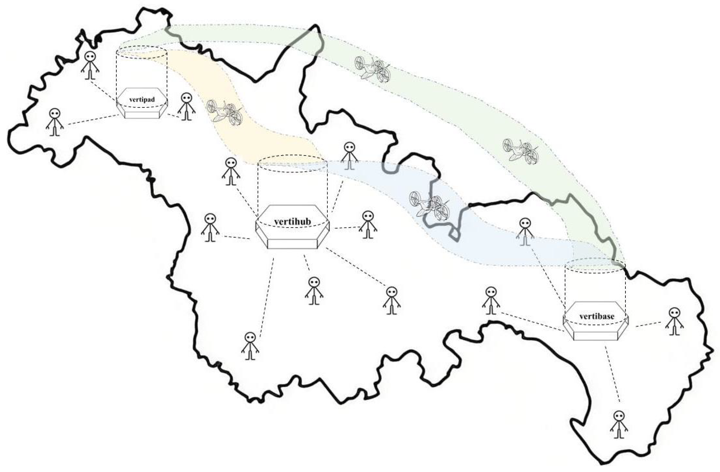
2.1. Problem Description

Vertiport location problem refers to the process of selecting suitable locations for constructing take-off and landing facilities for eVTOL aircraft, helicopters, and other aircraft in urban or suburban areas. Same-level vertiports have been considered in most of the current literature on the vertiport location problem; however, the distinction between different-level vertiports has a significant impact on the overall efficiency of the transportation system. Hence, this paper focuses on the location problem of hierarchical vertiports. Vertiports usually include infrastructure for taking off and landing, aircraft maintenance, and charging. They can be categorized into three levels—vertihub (high-level), vertibase (medium-level), and vertipad (low-level)—according to their construction scale and service capacity [26], as shown in Table 2. Therefore, based on the demand quantity and the construction conditions of the candidate vertiports, their locations and levels are determined, as shown in Figure 1. The area with high demand (center of Figure 1) is equipped with the high-level vertiport (vertihub), the area with moderate demand (bottom right of Figure 1) is equipped with the medium-level vertiport (vertibase), and the area with low demand (top left of Figure 1) is equipped with the low-level vertiport (vertipad). The above three levels (high, medium, and low) are considered for the vertiport classification scenarios in this paper.

2.2. Model Formulation

In most of the existing literature, the objective function of optimization models primarily considers the vertiport construction and passenger travel costs [19,20,21,22,23,24,25]. Building on previous studies, this paper introduces a penalty cost for exceeding capacity limits. We systematically establish a multi-dimensional cost control framework centered on investment efficiency, commute service, and utilization efficiency. This framework significantly reduces the overall construction cost of vertiports by optimizing location schemes. It also effectively improves passenger service satisfaction by minimizing commuting costs. Furthermore, by introducing the capacity-overload penalty mechanism, operational cost is constrained to improve the utilization efficiency of vertiport resources. While comprehensively considering the above factors, we quantitatively analyze the dynamic equilibrium among construction investment, commuting efficiency, and operational efficiency. Ultimately, a triple-win solution is achieved, balancing investors’ cost expenditures, passengers’ travel experiences, and service quality assurance. The objective function of the optimization problem P is as follows:
j J k K f k y j k + i I j J c i j d i x i j + g j J max i I d i x i j k K a k y j k , 0 ,
where I denotes the set of demand points; J is the set of candidate vertiports; K = { 0 , 1 , 2 } represents the set of vertiport levels; and k = 0 , k = 1 , and k = 2 correspond to low-level, medium-level, and high-level vertiports, respectively, f k represents the construction cost of a k-level vertiport, c i j denotes the distance cost from demand point i to candidate vertiport j, d i is the demand quantity at demand point i, g is the penalty factor, and a k represents the capacity of k-level vertiport. The decision variables x i j and y j k are binary variables. x i j takes the value 1 if demand point i is served by candidate vertiport j, and 0 otherwise. y j k takes the value 1 if k-level vertiport is established at candidate vertiport j, and 0 otherwise.
The first term in Equation (1) aims to calculate the total construction cost, considering economic benefits from the investor’s perspective. The second term aims to enhance travel convenience and efficiency, reduce passengers’ commuting burden, and ultimately improve the overall efficiency of the transportation system from a passenger-oriented perspective. The third term is about the relationship between vertiport capacity and demand quantity. To reduce passenger waiting time and improve overall operational efficiency, a penalty factor g is addressed when the demand exceeds the capacity limitation.
Considering the principle of proximity in assigning vertiports to each demand point, the single-assignment median location model for vertiports is addressed in this paper. That is, for each demand point i, there exists exactly one candidate vertiport j to service it. The service assignment constraints are formulated as follows:
j J x i j = 1 , i I .
Given that a vertiport of the specified level can be established at most for each candidate vertiport j, and that each vertiport must be constructed at candidate point j if it serves demand point i, the level assignment and service uniqueness constraints are formulated as follows:
k K y j k 1 , j J ,
x i j k K y j k , i I , j J ,
x i j { 0 , 1 } , i I , j J ,
y j k { 0 , 1 } , j J , k K .
The operational noise from vertiports may affect the health, well-being, and social stability of nearby residents, potentially resulting in public complaints, legal disputes, and even violations of environmental regulations. Therefore, the factor of noise-sensitive areas is incorporated into the model in this paper, with the following constraints:
y j k N j k , j J , k K ,
where the binary parameter N j k = 0 indicates that constructing a k-level vertiport is forbidden at candidate point j in noise-sensitive area; otherwise, N j k = 1 .
No-fly zones, such as military-controlled airspace or special flight restriction areas, are established to ensure national security, military activities, or emergency pathways. Any unauthorized location in these zones could lead to serious safety incidents or legal consequences. Therefore, the constraints regarding no-fly zones are formulated as follows:
k K y j k 1 e j , j J ,
where the binary parameter e j = 1 indicates that candidate vertiport j is in a no-fly zone; otherwise, e j = 0 .

2.3. Model Reformulation

Since the third term in the objective function (1) is nonlinear, this will lead to difficulties in solving the problem. Additionally, given that the decision variables are discrete, we adopt the Big-M method for linearization in this paper. Let z j = m a x { i I d i x i j k K a k y j k , 0 } , and binary variables u 1 j and u 2 j , as well as the following constraints, are incorporated,
i I d i x i j k K a k y j k z j , j J ,
z j i I d i x i j k K a k y j k + M ( 1 u 1 j ) , j J ,
z j M ( 1 u 2 j ) , j J ,
u 1 j + u 2 j 1 , j J .
In this linearization process, binary variables u 1 j and u 2 j are used to indicate the activation status of capacity constraints: when the total demand for candidate vertiport j exceeds its capacity (i.e., i I d i x i j > k K a k y j k ), constraints (10) enforce u 1 j = 1 and u 2 j = 0 , making z j exactly equal to the overload amount; otherwise, constraints (11) enforce u 1 j = 0 and u 2 j = 1 , setting z j to zero. Constraints (12) ensure that one of these two conditions must be met to avoid logical conflicts. Additionally, the value of M is calculated by the total demand M = i I d i across all demand points to ensure that M is sufficiently tight.
Then, the optimization model P is reformulated as follows:
P 1 : min j J k K f k y j k + i I j J c i j d i x i j + g j J z j ,
s . t . ( 2 ) ( 12 ) ,
z j 0 , j J ,
u 1 j { 0 , 1 } , j J ,
u 2 j { 0 , 1 } , j J ,
where the decision variables are x i j , y j k , z j , u 1 j , and u 2 j . Both the objective function and the constraint functions are linear.

3. Optimization Algorithm

As the number of candidate vertiports and demand points increases, the size of model P1 grows exponentially. Traditional exact algorithms often become infeasible for large-scale instances. In this paper, we incorporate the Lagrange relaxation technique and a variable neighborhood search (VNS) strategy within a branch-and-bound framework to construct the LVBB algorithm for solving the problem. The Lagrange relaxation technique can transform a large-scale problem into several parallel subproblems, thereby quickly obtaining a lower bound for model P1. The VNS strategy can avoid local optima, thus providing an effective upper bound for model P1.
The LVBB algorithm procedure is illustrated in Figure 2, where F represents the set of nodes formed by all non-integer variables. The maximum number of iterations is denoted by P, and the current upper and lower bounds of Model P1 are represented by Z ¯ and Z ̲ , respectively.

3.1. Lagrange Relaxation

In this paper, the Lagrange relaxation technique is applied to transform the demand allocation constraints (2) into weighted penalty terms in the objective function, thereby obtaining a high-quality lower bound for the model P1. The Lagrange relaxation model LR of Model P1 is formulated as follows:
LR : min j J k K f k y j k + i I j J c i j d i x i j + g j J z j + i I λ i 1 j J x i j ,
s . t . ( 3 ) ( 12 ) , ( 14 ) ( 16 ) ,
where λ i is the Lagrange multiplier.
In the LVBB algorithm, the binary variables x i j , y j k , u 1 j , and u 2 j are relaxed to the continuous variables, that is, the constraints (5), (6), (15), and (16) in LR model are transformed to constraints as (27), (28), (30), and (31). Meanwhile, based on the characteristics of the objective function and other constraints, Model LR can be transformed into parallel subproblems for each candidate vertiport j J :
LR j : min k K f k y j k + i I c i j d i x i j + g z j i I λ i x i j ,
s . t . k K y j k 1 ,
x i j k K y j k , i I ,
y j k N j k , k K ,
k K y j k 1 e j ,
i I d i x i j k K a k y j k z j ,
z j i I d i x i j k K a k y j k + M ( 1 u 1 j ) ,
z j M ( 1 u 2 j ) ,
u 1 j + u 2 j 1 ,
0 x i j 1 , i I ,
0 y j k 1 , k K ,
z j 0 ,
0 u 1 j 1 ,
0 u 2 j 1 .
By dynamically adjusting Lagrange multiplier λ i , the objective function optimization and constraint violation can be balanced. They play a crucial role in the rapid convergence of the branch-and-bound algorithm. In this paper, the subgradient method is used to update Lagrange multiplier λ = λ 1 , λ 2 , , λ I T ; the updating formula is as follows:
λ ( p + 1 ) = λ ( p ) + t ( p ) s ( p ) ,
where p is the iteration count and s ( p ) = s 1 ( p ) , s 2 ( p ) , , s | I | ( p ) T is the subgradient direction, in which s i ( p ) = 1 j J x i j * , t ( p ) = Z ¯ ( p ) Z ( p ) s ( p ) 2 is the step length of the subgradient method, x i j * represents the optimal solution of variable x i j , Z ¯ ( p ) denotes the upper bound of the objective function for Model P1 at the p-th iteration, Z ( p ) represents the optimal value of Model LR when the Lagrange multiplier is λ ( p ) at the p-th iteration.

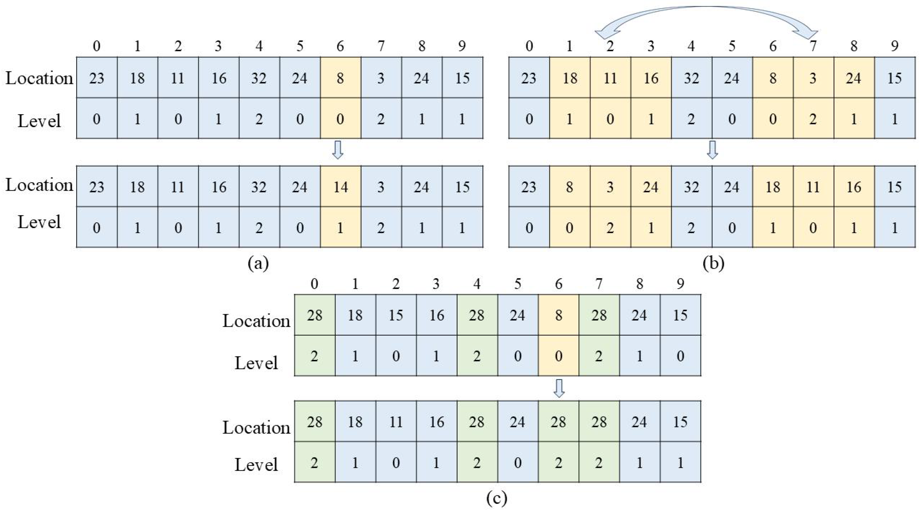
3.2. Variable Neighborhood Search

The framework of the VNS algorithm primarily consists of two parts: Variable Neighborhood Descent Search (VND) and shaking. In this paper, the solution of Model P1 is defined as a 3 × I array. The first row represents the index of demand points, the second row is the index of candidate vertiports, and the third row is the index of vertiport levels. An example of a location result is shown in Figure 3.
The VND strategies designed in this paper are as follows: (1) Randomly replace one column in the array, as shown in Figure 4a; (2) Randomly select two segments from the array and swap their positions, as shown in Figure 4b. The shaking procedure involves deleting the least-used candidate vertiport from the second row and reassigning the corresponding demand points to the candidate vertiport that appears most frequently, as shown in Figure 4c.
The computational burden of the LVBB algorithm primarily stems from three layers: solving Lagrangian-relaxed subproblems L R j in parallel, iteratively updating multipliers via the subgradient method, and neighborhood move operations in the variable neighborhood search. Although worst-case complexity remains exponential under the branch-and-bound framework, the decomposition strategy significantly enhances practical solving efficiency through parallel computing and localized search. Compared to typical methods, metaheuristic algorithms (e.g., genetic algorithm, Tabu search) exhibit polynomial complexity but may sacrifice optimality guarantees, while traditional exact solvers (e.g., CPLEX) face severe scalability bottlenecks in medium-to-large-scale instances. This highlights LVBB’s design value in striking a balance between efficiency and precision.

4. Experimental Design and Result Analysis

Currently, Nanjing in China has issued a series of implementation plans and policy measures to promote the high-quality development of the low-altitude economy, which include the deployment and planning of UAM systems [27]. Therefore, based on the above model and algorithm, we take the 11 administrative districts of Nanjing as an example to research the urban vertiports location problem. The model was implemented in Java and solved using the ILOG CPLEX 12.10 solver. The experimental environment was configured with an Intel(R) Core(TM) i7-8550U CPU, operating frequency of 1.80 GHz, 8.00 GB of RAM, and running on the Windows 10 (64-bit) operating system.

4.1. Experimental Design

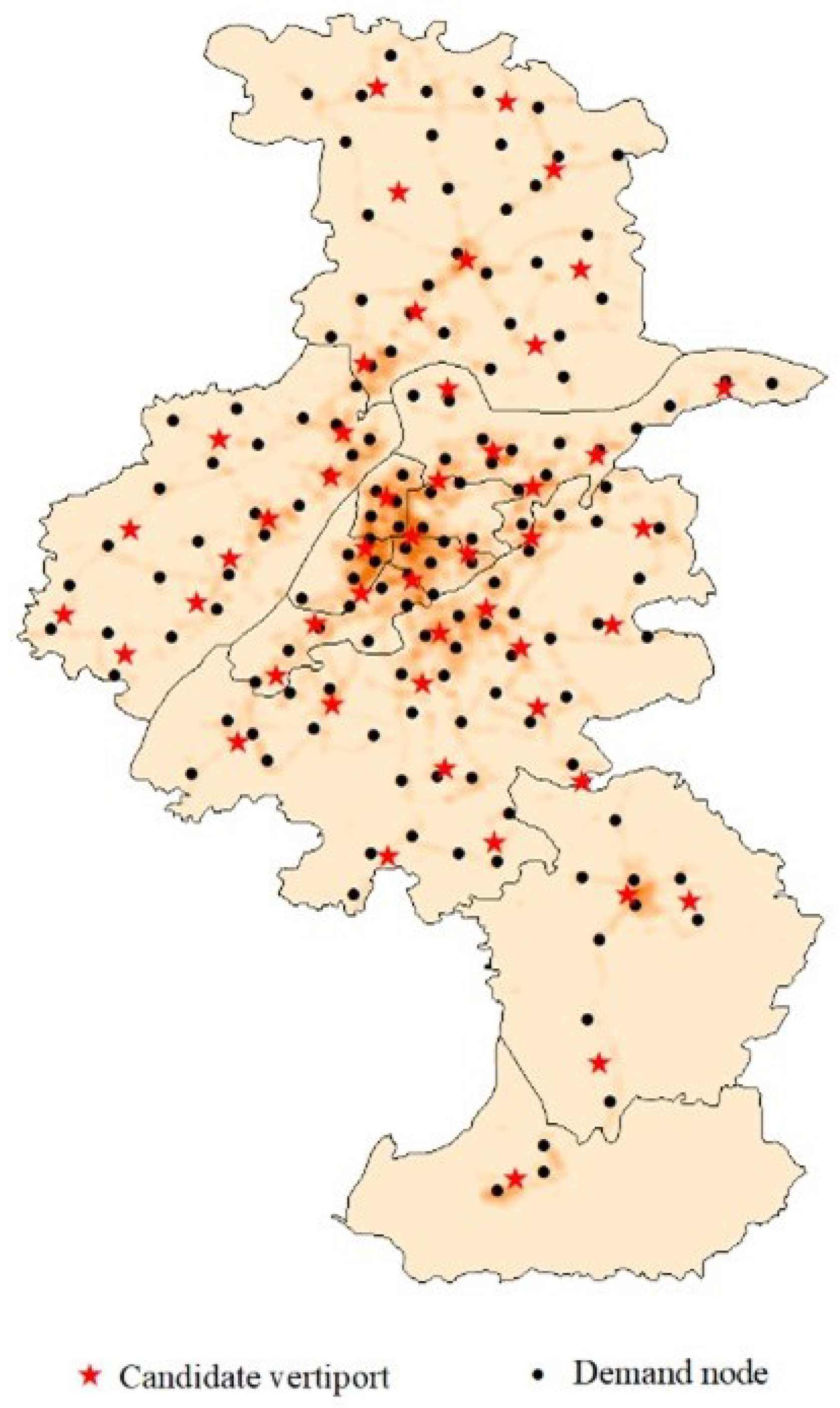
4.1.1. Selection of Candidate Vertiports and Demand Points

To ensure efficient connectivity and transitions between different modes of transportation, urban transportation stations are one of the optimal candidate vertiports. They guarantee the smooth implementation of multimodal transport and promote the development of the integrated urban transportation system. Therefore, we collect a total of 5634 data points from Nanjing’s subway stations, bus stops, and highway entrances/exits. According to Jeong’s work, São Paulo in Brazil, with a population of 21 million, plans to construct 100 vertiports [17]. Based on Nanjing’s population of approximately 9.55 million in 2023, the proportional relationship between population size and infrastructure quantity, and the city’s future development plans, 50 candidate vertiports are selected.
In this study, we downloaded data from Nanjing’s transportation stations from OSM (OpenStreetMap) and then applied the K-means algorithm to cluster. This process identified 50 candidate vertiports (as shown in Table 3) and 150 demand points (as shown in Figure 5). Most of these candidate vertiports are located near large parks, scenic areas, hospitals, or large buildings with suitable rooftops. However, some candidate vertiports have potential limitations. For example, Candidate Vertiport No. 17 is located near a school in a no-fly zone; Candidate Vertiport No. 22 is located in a residential area, where the operation of eVTOL aircraft may cause noise pollution.

4.1.2. Demand Quantity Setting

Because UAM systems in Nanjing are still in the planning phase, there are currently no publicly available operational data for UAM. Furthermore, demand quantity is influenced by multiple factors. Therefore, we adopt a comprehensive evaluation method to estimate the potential demand quantity.
For the vertiport location problem, Preis et al. considered key factors such as urban transportation stations, the urban economic development level (measured by GDP), the population of permanent residents, the area size, the number of companies, and others [28]. Accordingly, we selected three core evaluation indicators: the number of transportation stations ( N 1 ), urban GDP ( N 2 ), and the population of permanent residents ( N 3 ). The entropy weight method was applied to determine the weight of each indicator in the comprehensive evaluation system. The specific steps of the process are as follows:
First, normalize the original data. We use the vector normalization method, the expression of which is as follows:
a i j * = a i j i = 1 n a i j 2 , i = 1 , 2 , , n , j = 1 , 2 , , m ,
where a i j represents the original data, i is the evaluation object, and j is the evaluation indicator.
Next, calculate the feature weight of the i-th evaluation object under the j-th indicator:
p i j = a i j * i = 1 n a i j * , i = 1 , 2 , , n , j = 1 , 2 , , m .
Then, determine the difference coefficient g j = 1 e j for the j-th indicator by using the entropy value e j of the j-th indicator, which is calculated as e j = 1 ln n i = 1 n p i j ln p i j .
Finally, the weight coefficient for each indicator is
w j = g j k = 1 m g k , i = 1 , 2 , , n , j = 1 , 2 , , m .
According to the above method, the demand quantity for demand point i is calculated using the following formula:
d i = w 1 N 1 i + w 2 N 2 i + w 3 N 3 i ,
where N 1 i represents the number of transportation stations included in demand point i, N 2 i represents the GDP of the administrative district where demand point i is located, N 3 i represents the population of permanent residents in the administrative district where demand point i is located. The specific demand quantities at each demand point are listed in Table 4. In this paper, we assume that all passengers generated at each demand point are willing to use air transportation if such demand exists.
The selection of three core indicators—transportation station density (reflecting actual passenger flow), regional GDP (indicating business travel potential), and resident population (representing baseline travel demand)—comprehensively captures the key factors of UAM demand. The entropy weight method ensures that the final demand estimates comprehensively capture the combined effects of regional economics, population size, and transportation accessibility, ensuring the reliability of the experimental results.

4.1.3. Parameter Setting

In this paper, the distance cost c i j from demand point i to vertiport j is calculated based on the local taxi fare in Nanjing City: a base fare of 10 yuan (within 3 km), with an additional charge of 2.4 yuan per kilometer thereafter. According to China’s Road Traffic Safety Law, the permissible speed range for taxis on urban roads is 30–50 km/h. Thus, we set the taxi speed at 40 km/h as specified in the model parameters in this paper. The vertiports are divided into three levels, with corresponding construction costs provided by McKinsey Consulting Company [26], and their capacities within one day are set as shown in Table 5. Based on the discussion in Section 2.3, we set the Big-M value to Nanjing’s total demand, i.e., M = 205,784 . For the LVBB algorithm, the maximum iteration count P was set to 300, the maximum shaking count Q to 10, and the convergence threshold ϵ to 0.001.

4.2. Experimental Result and Analysis

Given the significant magnitude differences among construction cost, commuting cost, and penalty cost in the objective function, we apply max-min normalization to eliminate scale effects and enable balanced analysis. Each cost component Z k is transformed to [ 0 , 1 ] by using:
Z k n o r m = Z k Z k m i n Z k m a x Z k m i n , k = 1 , 2 , 3 ,
where Z k n o r m denotes the normalized cost components, and Z k m i n / Z k m a x are the minimum and maximum values, respectively, derived by solving optimization models containing solely the k-th cost term.

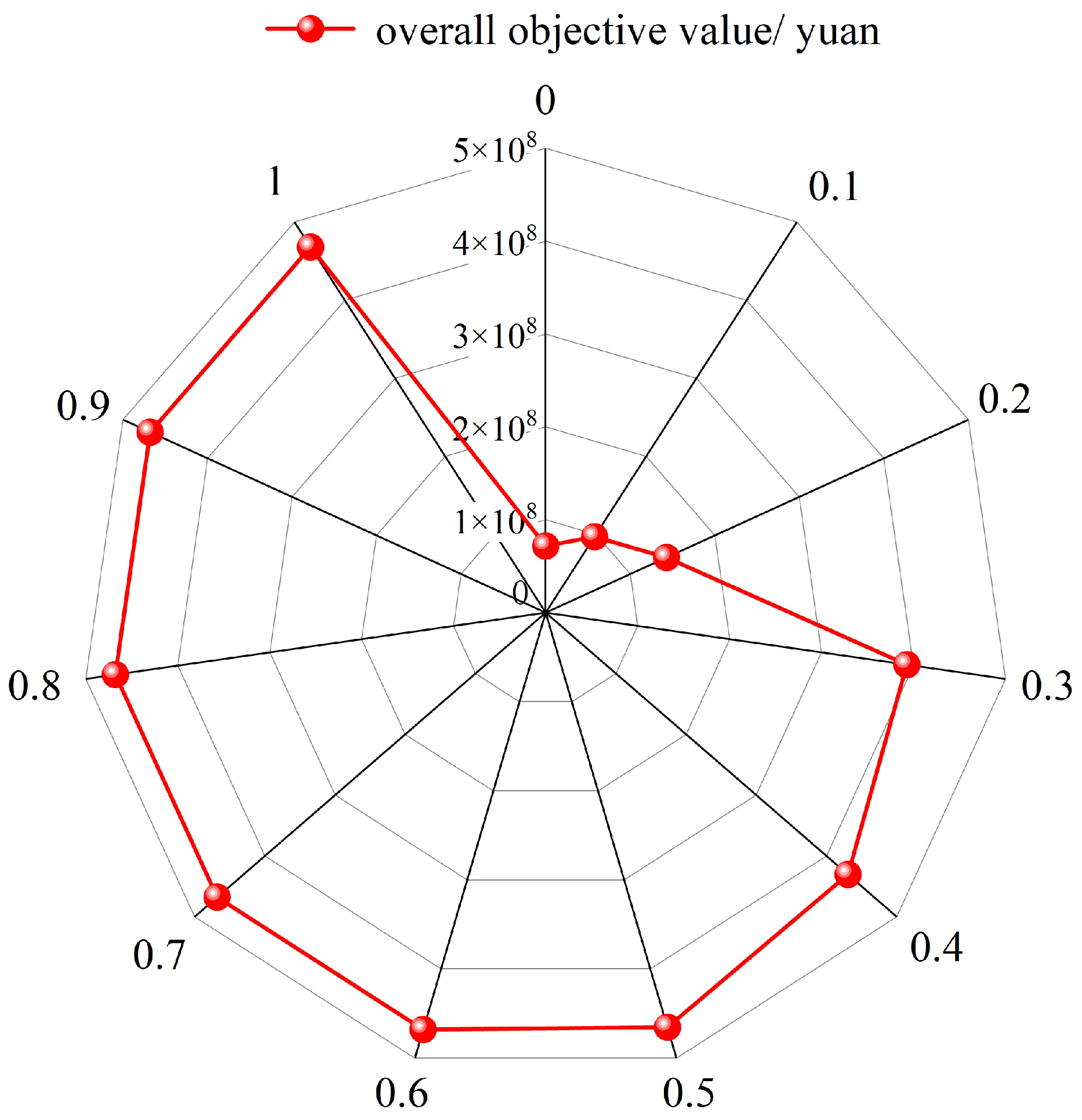
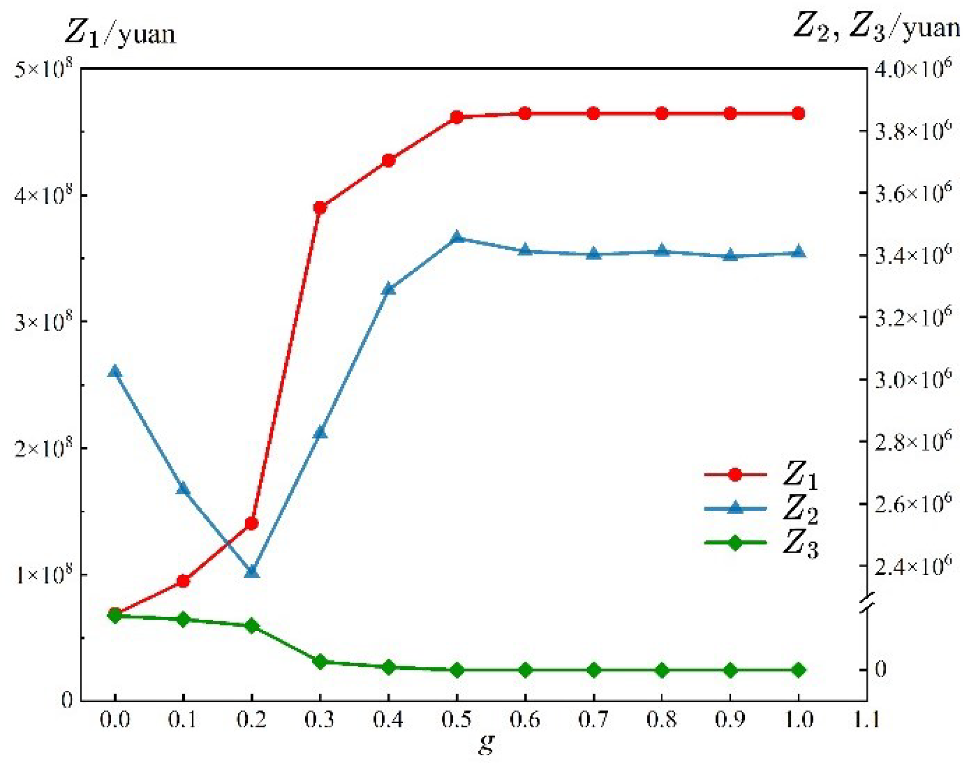
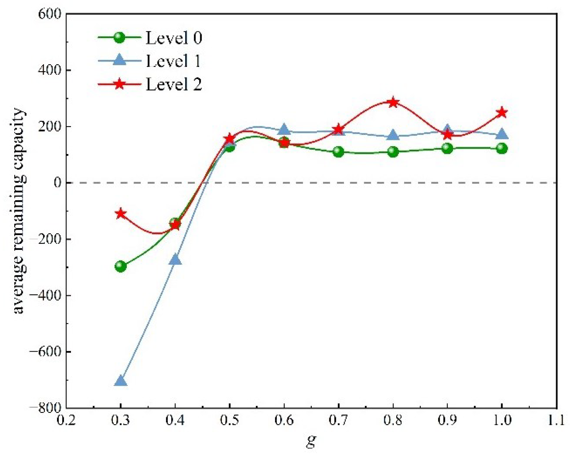
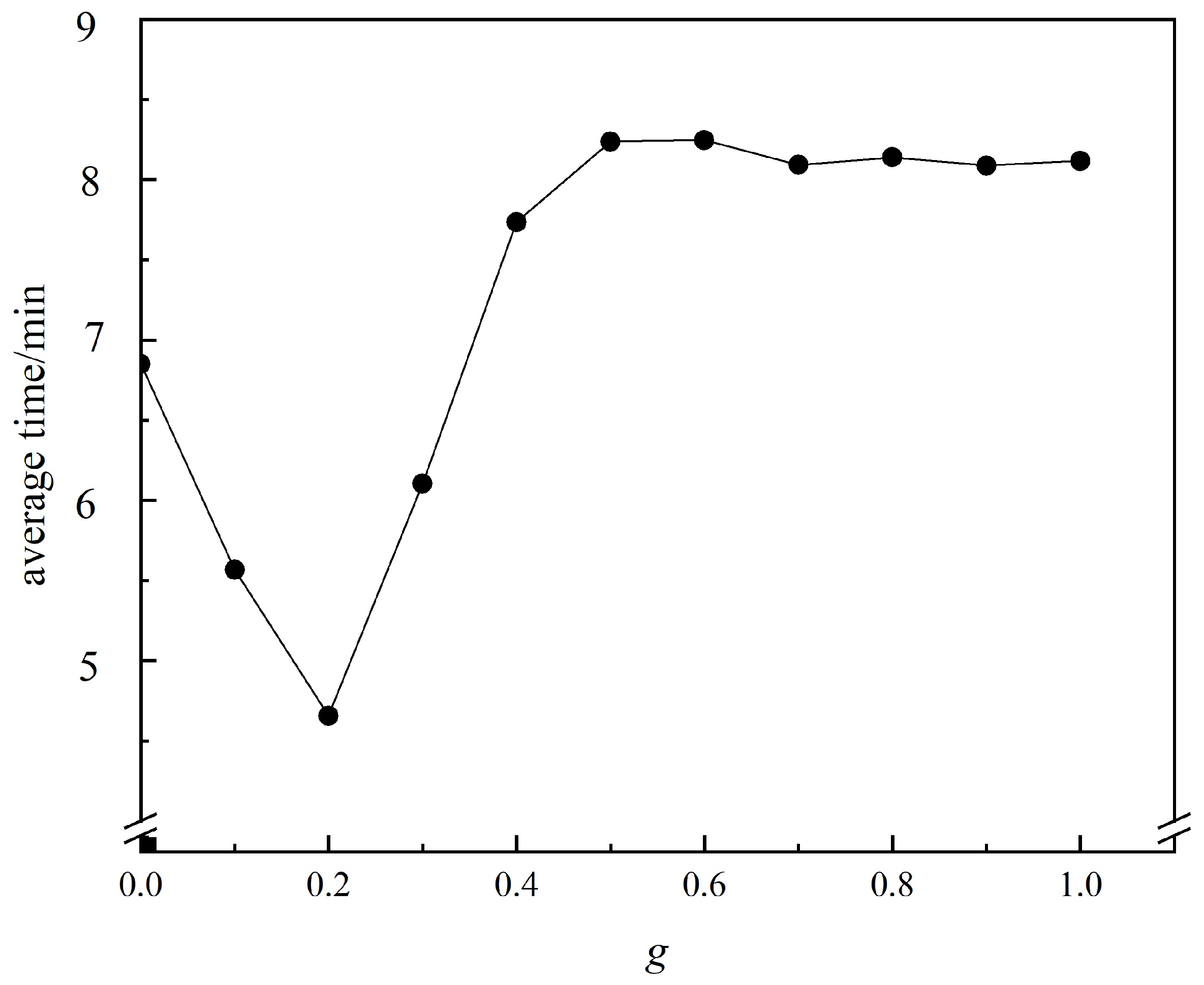
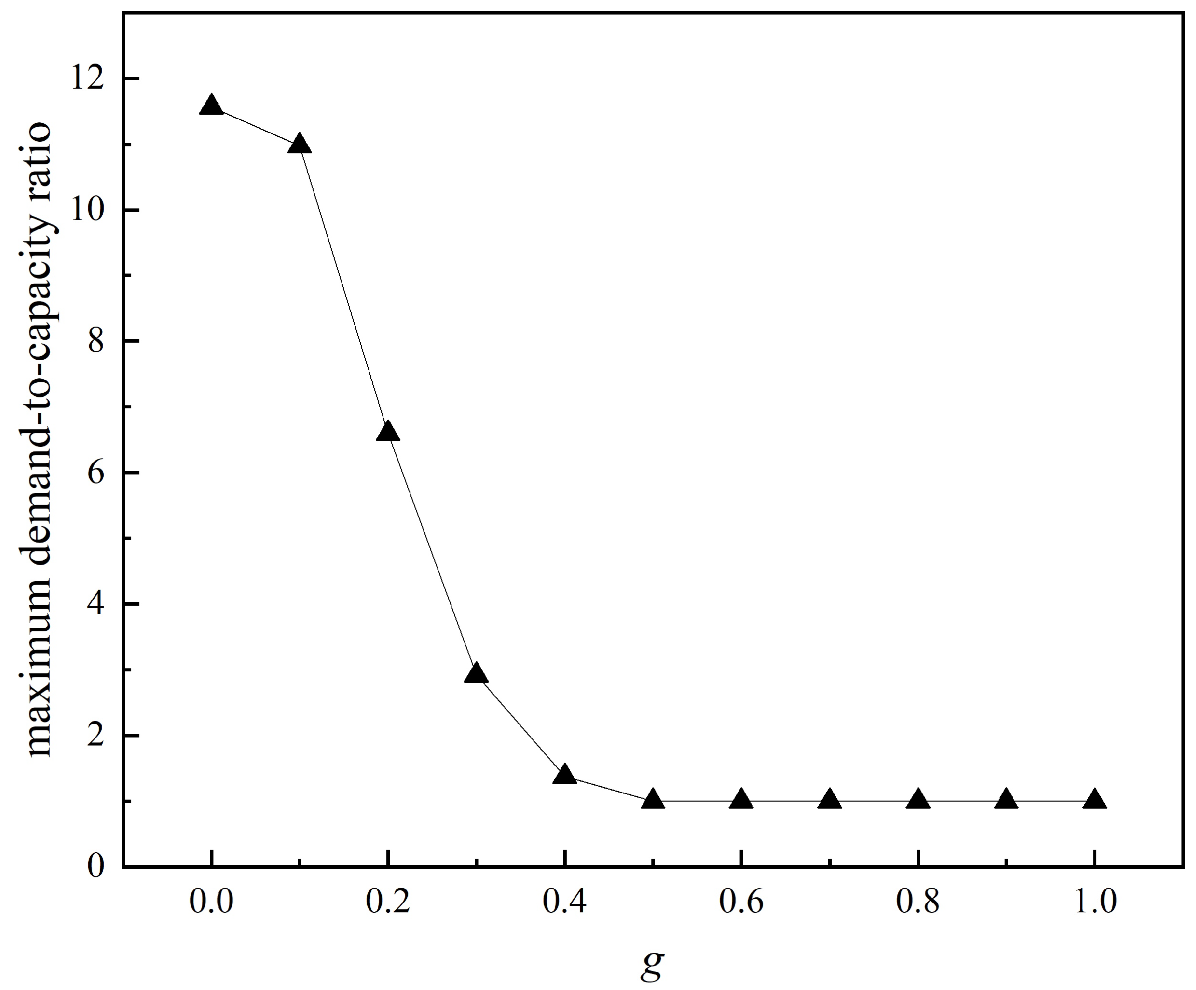
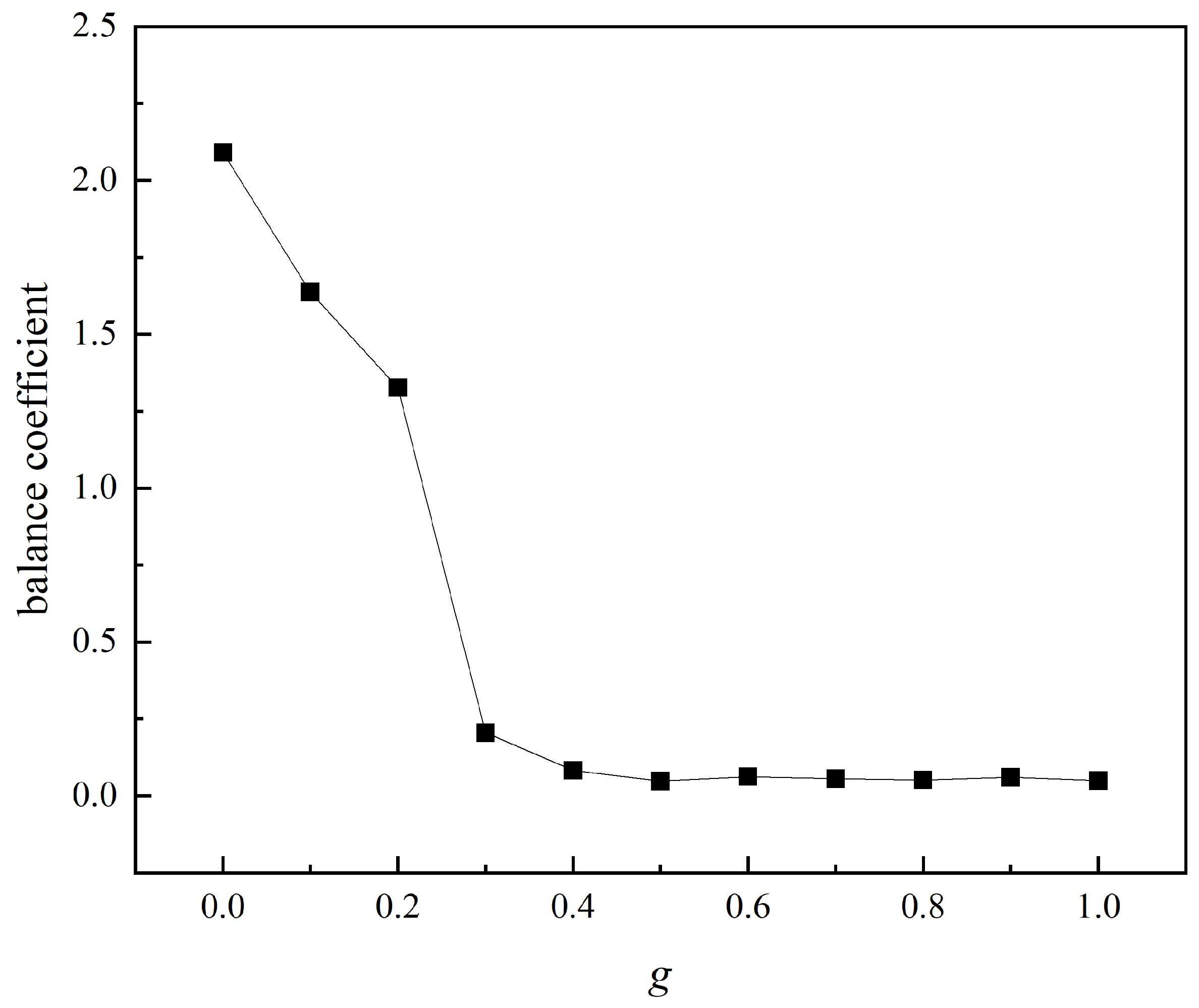
4.2.1. Analysis of the g-Value

Since the penalty factor g-value in the third term of the objective function in Model P1 affects the location results, we conduct a sensitivity analysis on the penalty factor g. Its value ranges from 0 to 1.0 (with an increment of 0.1). Figure 6 shows the number of each level of vertiports at different g-values.
As the penalty factor g increases, the capacity limitation requirement becomes increasingly stringent. In Figure 6, when the value of g is from 0 to 0.2, i.e., the capacity limitation requirement is relatively low—only 0-level vertiports are located, and the number of vertiports shows a significant upward trend, reaching its peak at g = 0.2 , with a total of 49 vertiports. During this phase, the system primarily meets the demand by increasing the number of 0-level vertiports. However, when the value of g exceeds 0.3, i.e., the capacity limitation requirement is moderate, the number of 0-level vertiports suddenly decreases. This change reflects that 1-level and 2-level vertiports more largely fulfil the demand as g increases. When the value of g exceeds 0.6, i.e., the capacity limitation requirement is high, the number of vertiports at each level gradually tends to stabilize.
The objective function (1) of Model P is divided into three parts: the first part Z 1 = j J k K f k y j k represents the construction cost of vertiport, the second part Z 2 = i I j J c i j d i x i j represents the commuting cost for passengers, and the third part Z 3 = j J max i I d i x i j k K a k y j k , 0 represents the penalty cost for capacity limitation. The effect of the penalty factor g on the overall objective function value Z = Z 1 + Z 2 + g Z 3 is shown in Figure 7. When 0 g 0.4 , as the penalty factor g gradually increases, the objective function value Z shows a significant upward trend; when g 0.5 , the objective function value Z tends to stabilize. Figure 8 illustrates the relationship among Z 1 , Z 2 and Z 3 at different g. As the penalty factor g increases, Z 1 shows an upward trend, which is due to the increase in the number of 1-level and 2-level vertiports, and the construction cost of these levels of vertiports is significantly higher than that of 0-level vertiports. In the process of increasing g from 0 to 0.2, Z 2 continues to decrease and reaches its minimum at g = 0.2 . Because the number of vertiports reaches its maximum, thereby effectively reducing the average distance between the demand point and the vertiport, to lower the commuting cost for passengers. However, as the penalty factor g further increases, the number of vertiports decreases and gradually stabilizes, which can lead to another increase in the commuting cost. For Z 3 , as the penalty factor g increases, it gradually decreases, which means that the capacity limitation of the vertiports is increasingly met. It is worth noting that when g 0.5 , Z 3 drops to zero, marking that the capacity limitation has been fully satisfied.
The average remaining capacity refers to the total remaining capacity of vertiports divided by the total number of vertiports. Numerical experiments in this paper show that the g-value has a significant impact on the average remaining capacity. When g < 0.3 , only 0-level vertiports are located and their capacity is far smaller than the demand quantity; the average remaining capacity is presented from g = 0.3 . As shown in Figure 9, when g < 0.5 , the remaining capacities of vertiports at all levels are negative, which indicates that the demand quantity exceeds the capacity. However, when g 0.5 , the capacities of vertiports at all levels meet the demand quantity. The average remaining capacities of 0-level and 1-level vertiports gradually stabilize, while the average remaining capacity of 2-level vertiports shows a fluctuating trend.
As the penalty factor g increases continuously, the corresponding passenger commuting time also experiences dynamic changes. To better understand this relationship, we further investigate how the average commuting time from demand points to their assigned vertiports varies at different g-values. The average time is defined as the total travel time between vertiports and their served demand points divided by the number of demand points. Figure 10 presents the average travel time across various g-values. When g increases from 0 to 0.2, the average time decreases significantly, reaching its minimum at g = 0.2 . This change is attributed to the relatively low penalty cost, which allows for a dense deployment of 0-level vertiports (a total of 49), thereby greatly reducing passenger access distances. However, as g exceeds 0.2, the average time gradually increases due to the reduction in the number of vertiports, and when g 0.5 , the average time gradually stabilizes.
The maximum demand-to-capacity ratio demonstrates a sharp exponential decay as penalty factor g increases, as shown in Figure 11. At g = 0 (no penalty), severe overload occurs with a ratio of 11.57, indicating the busiest vertiport is operating under a significant overload, exceeding its designed capacity by more than 11 times. As g rises to 0.3, the ratio plummets to 2.92, reflecting that the congestion is significantly relieved. The critical threshold emerges at g = 0.5 where the ratio reaches 0.99, achieving near-perfect demand-capacity equilibrium. Beyond this point, g 0.5 , the ratio is stabilized at nearly 1, confirming that all vertiports consistently operate within safe capacity limits while maintaining minimal resource redundancy.
To assess the spatial distribution of resource utilization and prevent localized congestion at some vertiports while others remain underutilized, we introduce the balance coefficient. This metric quantifies the deviation of individual vertiport demand-to-capacity ratios from the network-wide average ratio. It is calculated as
j J | Δ j μ | | J | ,
where Δ j represents the demand-to-capacity ratio at vertiport j and μ is the mean value of the ratios across all vertiports, exhibits dramatic phase changes with increasing g, as shown in Figure 12. When g = 0 (no penalty), a severe imbalance occurs (coefficient = 2.09) due to extreme demand–capacity disparities across vertiports. As g rises to 0.3, the coefficient plunges 90% to 0.205, indicating rapid convergence toward equilibrium. The optimal balance emerges at g = 0.5 (coefficient = 0.048), where all vertiports operate within a 4.8% deviation from the mean utilization rate. For g 0.5 , the coefficient stabilizes near 0.055, confirming the penalty mechanism’s success in maintaining persistent resource-load equilibrium while accommodating demand fluctuations.
Therefore, based on the above analysis of the effects of the penalty factor g on the number of vertiports, total cost, construction cost, passenger commuting cost, capacity limitation penalty cost, average remaining capacity of vertiports, average commuting time, maximum demand-to-capacity ratio and balance coefficient, setting g = 0.5 can effectively balance the needs of both investors and passengers.

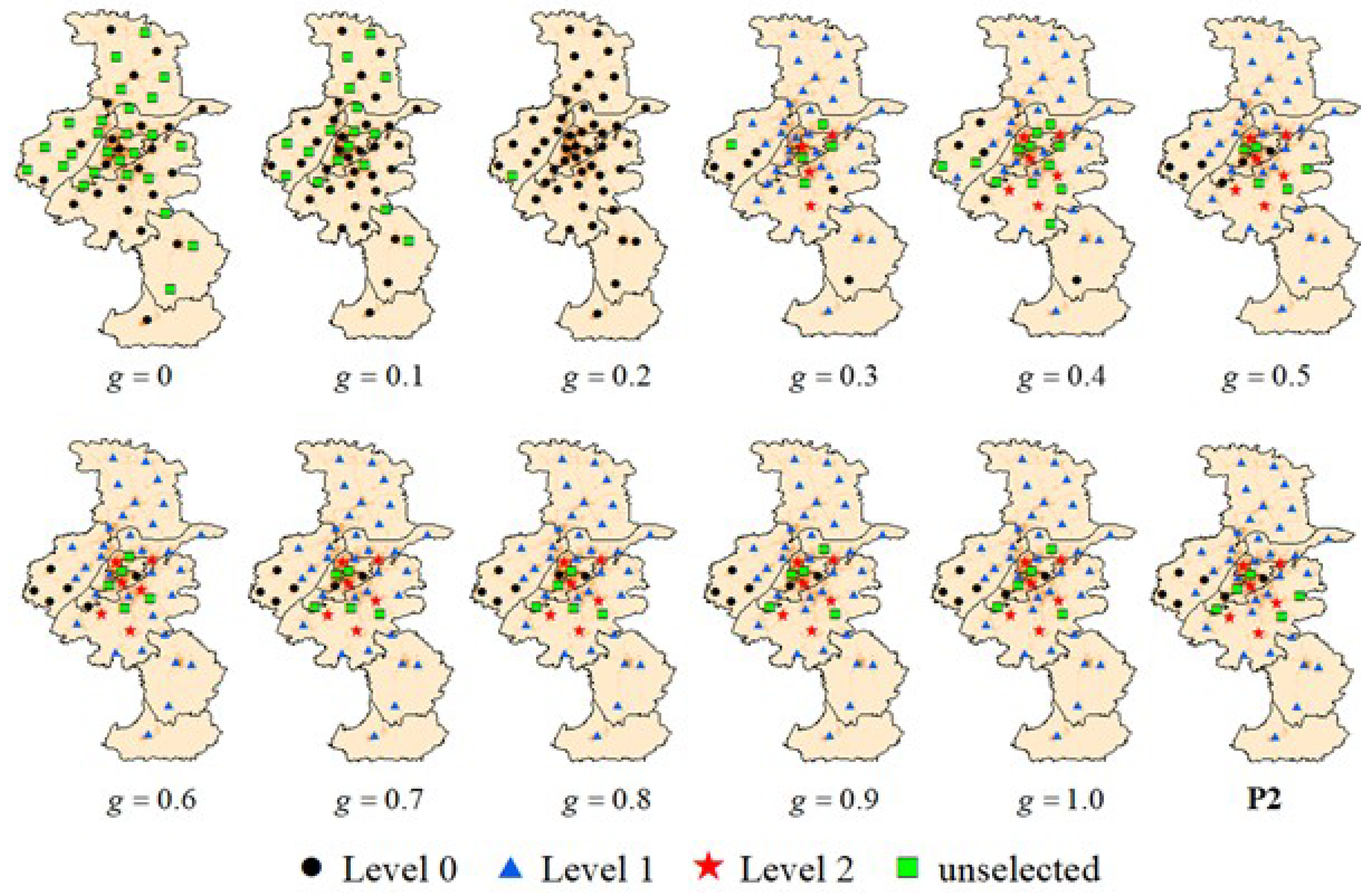
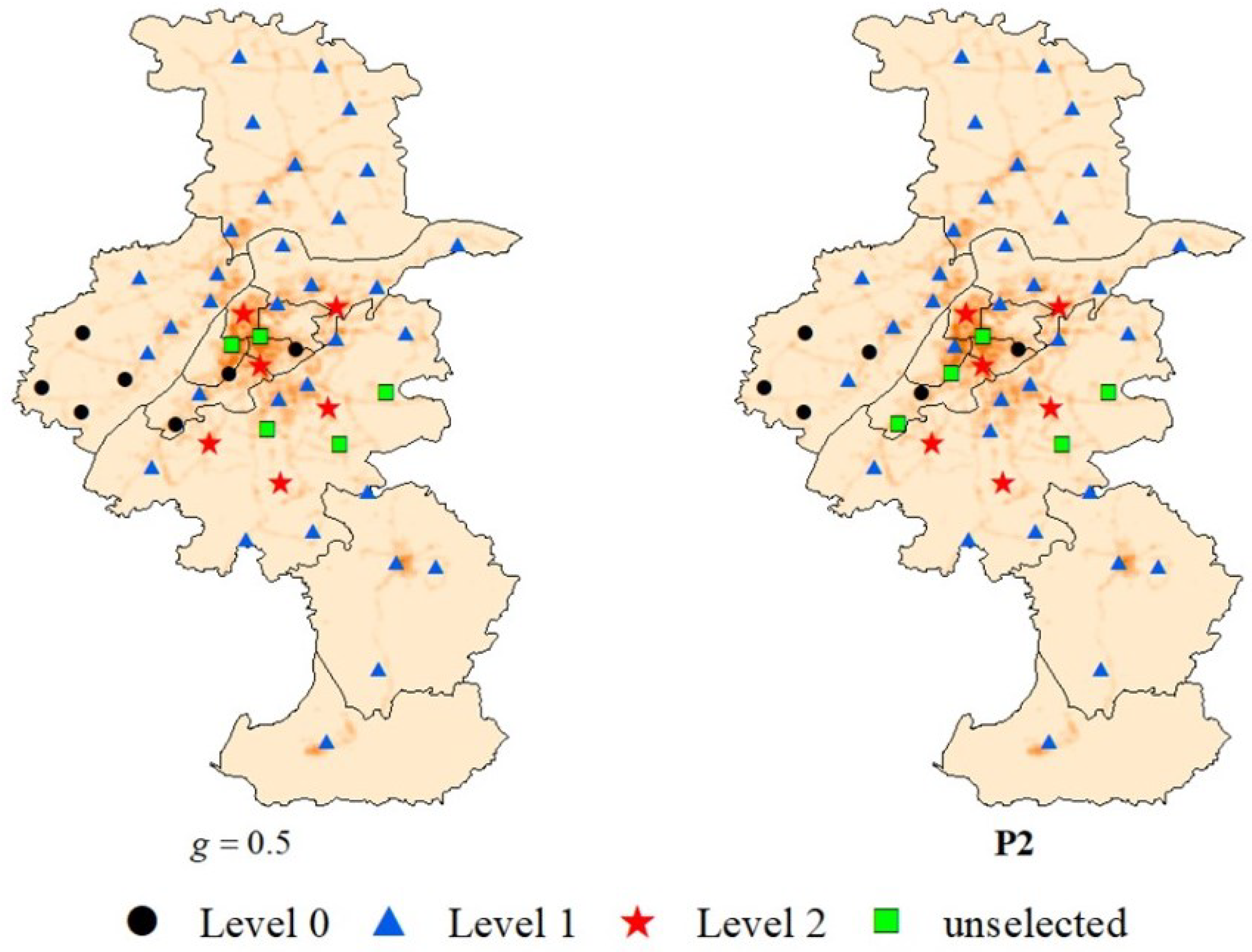
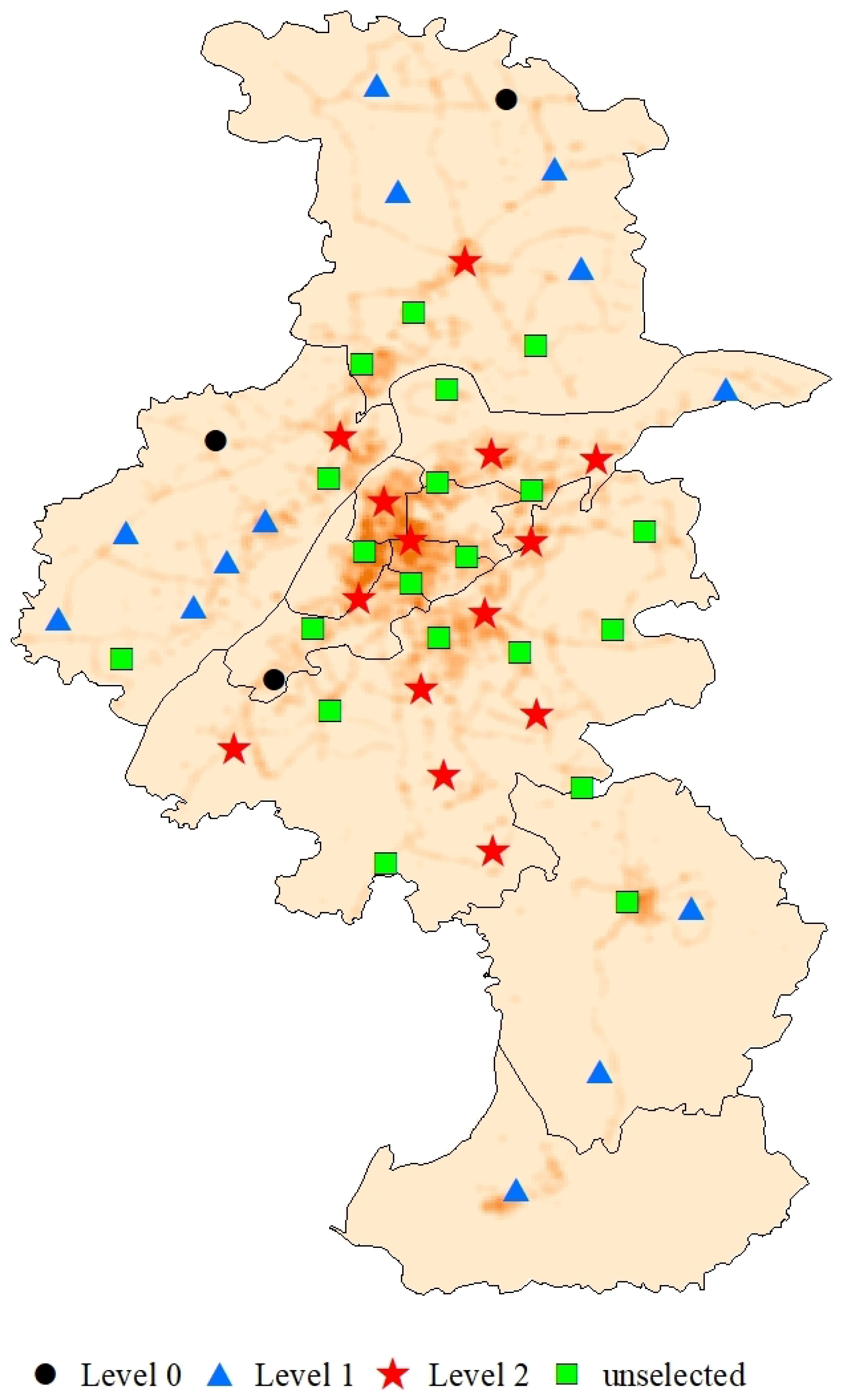
4.2.2. Location Visualization

The location results of vertiports at different g-values are shown in Figure 13 (green squares represent unselected vertiports, black circles represent 0-level vertiports, blue triangles represent 1-level vertiports, and red pentagrams represent 2-level vertiports). When g takes 0, 0.1, and 0.2, respectively, only 0-level vertiports are established, and their distribution aligns with the population density of Nanjing. This means that more vertiports are located in densely populated areas, while fewer are located in sparsely populated areas. As g increases, vertiports of all levels are located. 0-level vertiports are mainly located in the western regions of Nanjing City (Pukou District); 1-level vertiports are located in various administrative districts; 2-level vertiports are primarily located in the central regions of Nanjing City (Gulou District, Xuanwu District, Yuhuatai District). When g 0.5 , the number of vertiports remains consistent, and the geographical locations of vertiports are roughly the same. It is particularly noted that in the above location schemes, candidate vertiports No. 17 and No. 22 were not selected due to noise constraints and no-fly zone constraints.

4.2.3. Model Comparison

The capacity limitation in Model P1 is reflected through the third term about the penalty cost in the objective function. In addition, Model P2 is established with capacity constraints as follows:
P 2 : min j J k K f k y j k + i I j J c i j d i x i j ,
s . t . i I d i x i j k K a k y j k , j J , ( 2 ) - ( 8 ) ,
where constraint (40) indicates that for each candidate vertiport j, its capacity is greater than or equal to the corresponding demand quantity, ensuring that the vertiports meet the capacity constraint requirements. By comparing the location results of Models P1 and P2, the effectiveness of Model P1 is demonstrated.
According to the analysis of g-value in Section 4.2.1, when g = 0.5 , the location result not only meets the capacity requirements well but also has a lower cost. Therefore, the location result of Model P1 at g = 0.5 is compared with that of Model P2 in this section, as shown in Table 6. From Table 6, it can be seen that the total construction and commuting cost of Model P1 is approximately 2 × 10 6 yuan lower than those of Model P2. Additionally, under the condition of meeting capacity demands, Model P1 has less remaining capacity compared to Model P2, saving 29 units of average remaining capacity and avoiding resource waste. Figure 14 shows the location visualization of vertiports in Nanjing for both Model P1 at g = 0.5 and Model P2. It can be observed that the two location schemes are similar, with 2-level vertiports located in the central areas (Gulou District, Xuanwu District, Yuhuatai District), 1-level vertiports dispersed throughout Nanjing City, and 0-level vertiports mainly distributed in the central–western regions (Pukou District).
Based on the above analysis, the proposed Model P1 at g = 0.5 performs better than Model P2. It achieves a balance between meeting passenger demand and reducing construction costs.

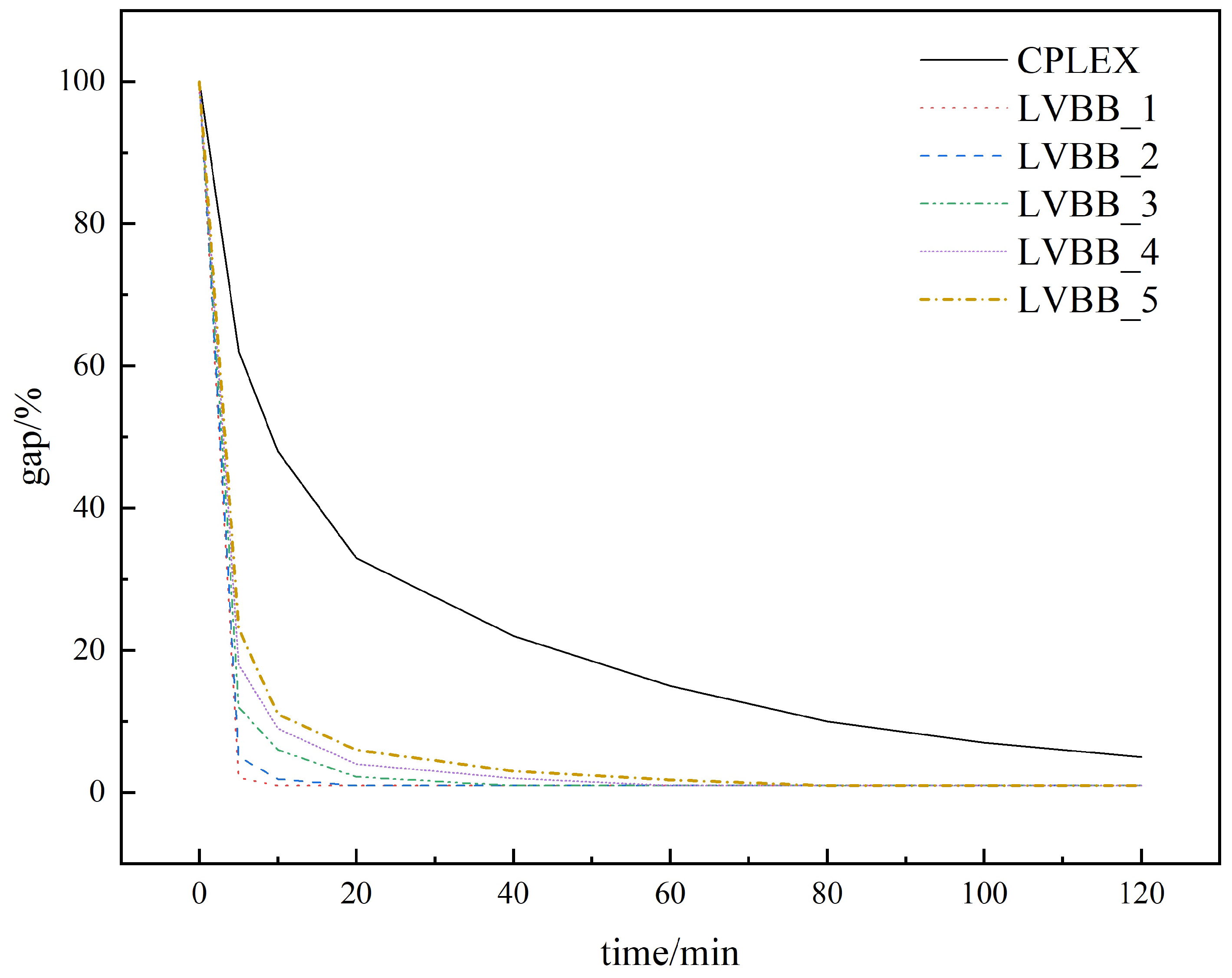
4.2.4. Computational Efficiency Analysis

Model P1 is a mixed integer programming (MIP) model, which is directly solved using the CPLEX solver. The computational efficiency of the CPLEX solver and the LVBB algorithm is compared for Model P1 ( g = 0.5 ). The CPLEX solver solving Model P1 ( g = 0.5 ) takes more than 2 h. In contrast, the LVBB algorithm with five different initial solutions (i.e., LVBB_1 to LVBB_5) takes no more than 2 h each. The average computational time is approximately 40 min. The experimental results are shown in Table 7. Figure 15 presents the relationship between the optimal gap and running time. As can be observed, the LVBB algorithm obtains superior solutions more rapidly than CPLEX. This indicates that the proposed LVBB algorithm significantly outperforms the CPLEX solver in terms of solution speed and effectiveness.

4.2.5. Utility Analysis of Air and Ground Transportation

In this paper, the five hotspots with the highest average daily taxi trip frequencies are selected in Nanjing, noting that Vertiports 18, 29, 33, 36, and 45 are located within these areas. Since all candidate vertiports are derived through clustering urban transportation stations, passengers can reach their respective vertiports via subways or buses. Therefore, only the trips between vertiports are considered in this section.
Based on the location scheme of Model P1 at g = 0.5 , it provides comparisons of travel time and cost for passengers using ground transportation versus air transportation (as shown in Figure 16) to reach their destinations. Public transportation refers to passengers choosing subways, buses, or a combination. The duration and cost data for public transportation and taxis are sourced from AutoNavi Maps. The cruising speed of eVTOL aircraft is set at 200 km/h, with costs estimated at approximately 6 yuan per kilometer based on the statements by Shanghai Autoflight Co., Ltd. (Shanghai, China).
In Table 8, the numbers in parentheses next to Origin (O)/Destination (D) represent the corresponding vertiport labels. In terms of travel time, air transportation can save approximately 90% of the travel time compared to public transportation and about 70% compared to taxis. In terms of travel cost, air transportation is more expensive than ground transportation. Specifically, the cost of air transportation is approximately 20 to 30 times that of public transportation, and about two or three times that of a taxi. This indicates that passengers who are more sensitive to time can choose air transportation to significantly reduce their travel time, while those who are more sensitive to cost can choose ground transportation to save on travel expenses.

4.2.6. Stochastic Analysis Under Uncertain Demand

To evaluate the model’s resilience to demand uncertainty, we extend Model P1 with a chance-constrained approach. By the Central Limit Theorem, we assume that demand d i follows a normal distribution d i N ( μ i , σ i 2 ) , where μ i is the expected demand from Table 4 and σ i = 0.5 μ i as an example. Then we introduce the chance constraints to guarantee service reliability:
P i I d i x i j k K a k y j k α , j J ,
where α is the confidence level. We set it as 0.90. By the deterministic equivalent transformation, these constraints are reformulated as:
i I μ i x i j + Φ 1 ( α ) i I σ i 2 x i j k K a k y j k , j J .
Since x i j are binary variables, the following relation is satisfied:
i I σ i 2 x i j = i I ( σ i x i j ) 2 i I σ i x i j 2 = i I σ i x i j .
To facilitate the solution process, we reformulate constraints (42) as follows:
i I μ i x i j + Φ 1 ( α ) i I σ i x i j k K a k y j k , j J .
Note that the reformulated constraints are tighter than the original constraints (42). In this case, the resulting vertiport location schematic diagram is as shown in Figure 17. It is not difficult to see that a total of 30 vertiports are established, including three 0-level vertiports, thirteen 1-level vertiports, and fourteen 2-level vertiports. The number of 2-level vertiports significantly exceeds that in the deterministic model. This is because more high-capacity vertiports are required to accommodate the fluctuating demand.

5. Conclusions

5.1. Contributions

This paper makes significant theoretical and practical contributions to hierarchical vertiport location optimization, which are summarized as follows:
(1)
The first hierarchical vertiport framework is introduced to address the gap in existing single-level, facility-focused literature.
(2)
A penalty mechanism is proposed to dynamically balance capacity overload and construction costs, with experimental results showing an optimal equilibrium at g = 0.5 .
(3)
To handle the nonlinear terms in the objective function, the Big-M method is applied for linearization. For the reformulated optimization model, an improved branch-and-bound algorithm (LVBB) is developed. It achieves faster computation effectiveness than CPLEX.
(4)
For numerical experiments, first, the K-means clustering algorithm is employed to determine the geographical locations of demand points and candidate vertiports. Then, a comprehensive evaluation method is used to estimate the demand quantity. Finally, numerical experiments are carried out using the LVBB algorithm on the reformulated model. The results show that the proposed location plan balances construction and commuting costs, improves vertiport utilization, and meets capacity requirements.
(5)
Robustness was verified via chance-constrained programming. Under demand fluctuations, the number of high-capacity vertihubs increased from 6 to 14, offering actionable insights for resilient infrastructure design.

5.2. Discussion

This solution provides an immediately actionable vertiport construction guide. Through a scientifically hierarchical vertiport framework, it achieves demand-adapted precision investment. Second, it employs a dynamic capacity penalty mechanism ( g = 0.5 ) to ensure demand-capacity balance, preventing resource waste. It then considers noise-sensitive and no-fly zones to enhance public acceptance. Ultimately, it establishes a comprehensive end-to-end implementation framework that encompasses hierarchical planning, elastic capacity allocation, and efficient simulation.

5.3. Limitations and Future Research

There are also some key limitations and research directions to consider:
(1)
The demand estimation was based on entropy weighting without validation from real-world UAM travel data. Future research should incorporate multi-source data (e.g., mobile signaling records, ride-hailing platform data) to enhance the accuracy of demand forecasting.
(2)
Although the LVBB algorithm outperforms CPLEX, systematic comparisons with state-of-the-art heuristics such as NSGA-III and Tabu Search are still needed to fully evaluate its solution quality and computational efficiency.
(3)
Stochastic construction cost, distance cost, and flight time were not considered. Robust optimization or stochastic programming should be incorporated to enhance model resilience.
(4)
Future studies should jointly optimize ground-air connectivity (e.g., metro/bus interchange) for integrated urban mobility.
(5)
Static demand allocation assumptions overlook real-time fluctuations and disruptions (e.g., weather-related route adjustments). Online optimization strategies are recommended for practical deployment.
(6)
Future research could introduce multi-objective Pareto optimization to simultaneously balance construction cost, passenger commute time, and capacity utilization, generating diversified location schemes for enhanced decision support.

Author Contributions

Conceptualization, Y.G., J.Y., J.J. and D.Q.; methodology, Y.G. and J.Y.; software, J.Y.; validation, Y.G. and J.Y.; formal analysis, Y.G., J.Y. and J.J.; investigation, J.Y. and J.J.; resources, Y.G. and D.Q.; data curation, J.Y and J.J.; writing—Original draft preparation, Y.G. and J.Y.; writing—review and editing, Y.G. and J.Y.; visualization, J.Y.; supervision, Y.G.; project administration, Y.G.; funding acquisition, Y.G. All authors have read and agreed to the published version of the manuscript.

Funding

This research was funded by a horizontal research project (No. KFA24538).

Data Availability Statement

The data presented in this study are available on request from the second author.

Conflicts of Interest

The authors declare no conflicts of interest.

Abbreviations

The following abbreviations are used in this manuscript:
UAMUrban Air Mobility
eVTOLelectric vertical takeoff and landing
LVBBLagrange relaxation-Variable neighborhood Branch-and-Bound
VNSVariable Neighborhood Search
VNDVariable Neighborhood Descent

References

  1. Qin, R.; Li, W.; Jin, J. Low altitude economy based on resource-based view. J. Civ. Aviat. Univ. China 2011, 29, 56–60. [Google Scholar]
  2. The Central People’s Government of the People’s Republic of China. The State Council of the Central Committee of the Communist Party of China issued the Outline of the National Comprehensive Stereoscopic Transportation Network Plan. 2021. Available online: https://www.gov.cn/zhengce/2021-02/24/content_5588654.htm (accessed on 9 October 2024).
  3. The Central People’s Government of the People’s Republic of China. Report on the Work of the Government. 2024. Available online: https://www.gov.cn/gongbao/2024/issue_11246/202403/content_6941846.html (accessed on 9 October 2024).
  4. Cohen, A.P.; Shaheen, S.A.; Farrar, E.M. Urban Air Mobility: History, Ecosystem, Market Potential, and Challenges. IEEE Trans. Intell. Transp. Syst. 2021, 22, 6074–6087. [Google Scholar] [CrossRef]
  5. Thipphavong, D.P.; Apaza, R.; Barmore, B. Urban air mobility airspace integration concepts and considerations. In Proceedings of the 2018 Aviation Technology, Integration, and Operations Conference, Atlanta, GA, USA, 25–29 June 2018; p. 3676. [Google Scholar]
  6. Wei, Q.; Gao, Z.; Clarke, J. Risk-aware urban air mobility network design with overflow redundancy. Transp. Res. Part B Methodol. 2024, 185, 102967. [Google Scholar] [CrossRef]
  7. Zheng, X.; Li, Z. Research progress and trends of urban air mobility. Flight Dyn. 2025, 43, 10–18. [Google Scholar]
  8. Brunelli, M.; Ditta, C.; Postorino, M. New infrastructures for Urban Air Mobility systems: A systematic review on vertiport location and capacity. J. Air Transp. Manag. 2023, 112, 102460. [Google Scholar] [CrossRef]
  9. Charnsethikul, C.; Silva, J.; Verhagen, W. Urban Air Mobility Aircraft Operations in Urban Environments: A Review of Potential Safety Risks. Aerospace 2025, 12, 306. [Google Scholar] [CrossRef]
  10. Yunus, F.; Casalino, D.; Avallone, F. Efficient prediction of urban air mobility noise in a vertiport environment. Aerosp. Sci. Technol. 2025, 139, 108410. [Google Scholar] [CrossRef]
  11. Kierzkowski, A.; Dziewoński, B.; Kaliszuk, K. Evaluation of Light Electric Flying-Wing Unmanned Aerial System Energy Consumption During Holding Maneuver. Energies 2025, 18, 1300. [Google Scholar] [CrossRef]
  12. Meng, L.; Wu, M.; Wen, X. Optimization of Flight Scheduling in Urban Air Mobility Considering Spatiotemporal Uncertainties. Aerospace 2025, 12, 413. [Google Scholar] [CrossRef]
  13. Wang, Y.; Li, J.; Yuan, Y. Joint Optimization of Cost and Scheduling for Urban Air Mobility Operation Based on Safety Concerns and Time-Varying Demand. Aerospace 2024, 11, 861. [Google Scholar] [CrossRef]
  14. Cunningham, E.; Healy, J.; Cuffe, P. An Analysis of the Feasibility of Providing On-demand Ground Level Illumination from a Loitering Unmanned Aerial Vehicle. In Proceedings of the 2024 IEEE International Workshop on Technologies for Defense and Security (TechDefense), Naples, Italy, 11–13 November 2024; pp. 86–91. [Google Scholar]
  15. Shao, Q.; Shao, M.; Lu, Y. Terminal area control rules and eVTOL adaptive scheduling model for multi-vertiport system in urban air Mobility. Transp. Res. Part C Emerg. Technol. 2021, 132, 103385. [Google Scholar] [CrossRef]
  16. Jin, Z.; Ng, K.; Zhang, C. Robust optimisation for vertiport location problem considering travel mode choice behaviour in urban air mobility systems. J. Air Transp. Res. Soc. 2024, 2, 100006. [Google Scholar] [CrossRef]
  17. Jeong, J.; So, M.; Hwang, H. Selection of vertiports using k-means algorithm and noise analyses for urban air mobility (UAM) in the seoul metropolitan area. Appl. Sci. 2021, 11, 5729. [Google Scholar] [CrossRef]
  18. Sinha, A.; Rajendran, S. A novel two-phase location analytics model for determining operating station locations of emerging air taxi services. Decis. Anal. J. 2022, 2, 100013. [Google Scholar] [CrossRef]
  19. Wu, Z.; Zhang, Y. Integrated network design and demand forecast for on-demand urban air mobility. Engineering 2021, 7, 473–487. [Google Scholar] [CrossRef]
  20. Shin, H.; Lee, T.; Lee, H. Skyport location problem for urban air mobility system. Comput. Oper. Res. 2022, 138, 105611. [Google Scholar] [CrossRef]
  21. Chen, L.; Wandelt, S.; Dai, W. Scalable vertiport hub location selection for air taxi operations in a met-ropolitan region. INFORMS J. Comput. 2022, 34, 834–856. [Google Scholar] [CrossRef]
  22. Jiang, Y.; Li, Z.; Wang, Y. Vertiport location for eVTOL considering multidimensional demand of urban air mobility: An application in Beijing. Transp. Res. Part Policy Pract. 2025, 192, 104353. [Google Scholar] [CrossRef]
  23. Petit, V.; Ribeiro, M. Multi-objective vertiport location optimization for a middle-mile package delivery framework: Case study in the South Holland Region. J. Air Transp. Manag. 2024, 125, 102757. [Google Scholar] [CrossRef]
  24. Willey, L.; Salmon, J. A method for urban air mobility network design using hub location and subgraph isomorphism. Transp. Res. Part C Emerg. Technol. 2021, 125, 102997. [Google Scholar] [CrossRef]
  25. Kai, W.; Jacquillat, A.; Vaze, V. Vertiport planning for urban aerial mobility: An adaptive discretization approach. Manuf. Serv. Oper. Manag. 2022, 24, 3215–3235. [Google Scholar] [CrossRef]
  26. Johnston, T.; Riedel, R.; Sahdev, S. To Take off, Flying Vehicles First Need Places to Land. New York. 2020. Available online: https://www.mckinsey.com/industries/automotive-and-assembly/our-insights/to-take-off-flying-vehicles-first-need-places-to-land (accessed on 23 December 2024).
  27. Nanjing Municipal People’s Government. Notice of the General Office of the Municipal Government on the Issuance of the Implementation Plan for Promoting the High-Quality Development of Low Altitude Economy in Nanjing (2024–2026). 2024; [EB/OL]. Available online: https://www.nanjing.gov.cn/zzb/zfxxgk/fdzdgknr/szfjbgtwj/202405/t20240514_4666425.html (accessed on 26 August 2024).
  28. Preis, L. Quick sizing, throughput estimating and layout planning for VTOL aerodromes–a methodology for vertiport design. In Proceedings of the AIAA Aviation 2021 Forum, Virtual, 2–6 August 2021; p. 2372. [Google Scholar]
Figure 1. Location of hierarchical vertiports.
Aerospace 12 00672 g001
Figure 2. Flowchart of LR-VNBB algorithm.
Aerospace 12 00672 g002
Figure 3. Example of location result.
Aerospace 12 00672 g003
Figure 4. VND strategies and shaking procedure. (a) Randomly replace one column; (b) Randomly select two segments and swap them; (c) Shaking procedure.
Aerospace 12 00672 g004
Figure 5. K-means clustering results diagram.
Aerospace 12 00672 g005
Figure 6. Number of vertiports at different g-values.
Aerospace 12 00672 g006
Figure 7. Relationship between g and the overall objective function value.
Aerospace 12 00672 g007
Figure 8. Relationship between g and the objective function value for each component.
Aerospace 12 00672 g008
Figure 9. Relationship between g and the average remaining capacity of vertiports.
Aerospace 12 00672 g009
Figure 10. Relationship between g and the average time.
Aerospace 12 00672 g010
Figure 11. Relationship between g and the maximum demand-to-capacity ratio.
Aerospace 12 00672 g011
Figure 12. Relationship between g and the balance coefficient.
Aerospace 12 00672 g012
Figure 13. Visualization of the vertiport location in Nanjing.
Aerospace 12 00672 g013
Figure 14. Visualization of location for Model P1 at g = 0.5 and Model P2.
Aerospace 12 00672 g014
Figure 15. Gap–time comparison between CPLEX and LVBB algorithms.
Aerospace 12 00672 g015
Figure 16. Diagram of transportation modes.
Aerospace 12 00672 g016
Figure 17. Visualization of location for stochastic model.
Aerospace 12 00672 g017
Table 1. Details of modeling optimization method in the literature.
AuthorObjectConstraintSolution Method
Wu, et al. [19]minimize the monetized time value and travel costvertiport count, mode exclusivity, economic feasibilityGurobi
Shin, et al. [20]minimize the travel cost, facility cost, and collision risk costthe nearest skyport, collision feasibilityGenetic Algorithm
Chen, et al. [21]minimize total travel costsingle allocation, flow balanceGrid-VNS
Jiang, et al. [22]maximize the coverage of on-demand mobility demand, regular shuttle demand, and congestion alleviation, minimize the redundant coverage of regular shuttlefacility capacity, socioeconomic limitation, minimum spacingNSGA-III
Petit, et al. [23]minimize the fraction of demand not served, minimize the sum of safety scores, minimize the sum of noise scoresvertiport count, coverage capability, capacity, safety distance, airspace restrictionmulti-objective Tabu Search
Willey, et al. [24]maximize the reduction in passenger travel time compared to ground transportationhub count, closest hub allocation, connectivity, time savings requirement, subgraph structurefive heuristic algorithms
Kai, et al. [25]maximize total profitdemand matching, queuing networkadaptive discretization algorithm
Table 2. Vertiport classification.
Vertiport LevelDescription
vertihub (high-level)Vertihub is established mainly in areas with high traffic flow (e.g., city center) and has about 10 take-off and landing platforms and 20 parking or maintenance platforms, as well as shopping and other services for passengers.
vertibase (medium-level)Vertibase is primarily established in areas with moderate traffic flow (e.g., office building, supermarket) and has about three take-off and landing platforms and six parking or maintenance platforms.
vertipad (low-level)Vertipad is established mainly in areas with low traffic flow (e.g., suburban area) and has approximately one take-off and landing platform and two parking or maintenance platforms.
Table 3. Candidate vertiports’ geographic location information.
No.Latitude & LongitudeGeographical LocationNo.Latitude & LongitudeGeographical Location
0(118.751003° N, 32.076942° E)Nanjing Ding Shan Garden Hotel25(118.753051° N, 31.690457° E)Qixian Mountain Rose Garden
1(119.010477° N, 31.469133° E)Menghuayuan Scenic Area26(118.903008° N, 31.911857° E)Ledongli Jiangning Digital Sports Center
2(118.734453° N, 32.528839° E)Phoenix Reservoir27(118.539931° N, 31.965801° E)Qionghua Lake Park
3(118.780373° N, 31.880843° E)Shuichang Street Vehicle Base28(118.85328° N, 32.063511° E)Zhongshan Scenic Area
4(119.025304° N, 32.051312° E)Tangshan Happy Water World29(119.013071° N, 31.648975° E)Shitang Reservoir
5(119.075445° N, 31.636296° E)Zhongshan Reservoir30(118.997365° N, 31.942594° E)Nanjing Chaopeng Logistics Co., Ltd.
6(118.838561° N, 32.336404° E)Wanda Plaza (Luhe Store) Phase I31(118.725989° N, 31.976911° E)Tongyue Valley Family Park
7(118.421888° N, 31.943368° E)Wancheng Ecological Park32(118.85547° N, 32.52002° E)Zhaoqiao Reservoir
8(118.820442° N, 31.923056° E)Jiangning Golden Eagle33(118.834481° N, 32.006183° E)Qiqiao Weng Ecological Wetland Park
9(118.589911° N, 31.825354° E)Binjiang New Town Park34(118.627258° N, 31.89677° E)Nanjing Meishan Hospital
10(118.724075° N, 32.246659° E)Duwei Wetland Park35(118.779359° N, 32.004173° E)Yuhuatai Scenic Area
11(118.579119° N, 32.005996° E)Nanjing LinDa Ecological Park36(118.921453° N, 32.25601° E)Hongshanyao Scenic Area
12(118.875531° N, 31.731864° E)Nanjing Lukou Airport37(118.814199° N, 32.006282° E)Nanjing Airport Logistics Center
13(118.806841° N, 32.092823° E)Cross-shaped Cypress Forest Park38(118.465652° N, 31.936634° E)Lingquan Fugui Scenic Area
14(118.939031° N, 32.428805° E)Jinniu Lake Hospital39(118.661313° N, 32.108797° E)Buddha Hand Lake Country Park
15(118.899471° N, 32.034937° E)Nanwan Ying Park40(118.701338° N, 32.376512° E)Chisong Lake National Wetland Park
16(118.897912° N, 31.337092° E)Wujiazu Legal Culture Park41(119.121375° N, 32.15936° E)Shui Yifang Ecological Leisure Tourism Area
17(118.911981° N, 31.850795° E)Longdu Town Fenqian Primary School42(118.781183° N, 32.286663° E)Jinshan Building Materials and Furniture City
18(118.728521° N, 32.177187° E)Datang Jin Fragrant Grass Valley43(118.893572° N, 32.092955° E)Nanjing Jiangning Hospital
19(118.784352° N, 32.178177° E)Nanjing First Hospital44(118.873448° N, 32.129654° E)Taiping Mountain Park
20(118.703775° N, 32.151846° E)Southeast University Chengxian College45(118.616187° N, 32.057481° E)Qiuyushan Cultural Park
21(118.990617° N, 32.306321° E)Fangshan46(118.666341° N, 31.938391° E)Redsun Home Expo Center
22(118.776935° N, 32.040071° E)Tongyu Garden47(118.998881° N, 31.758726° E)Daren Mountain Life Park
23(118.986025° N, 32.126679° E)Nanjing Xianlin Lake Park48(118.480984° N, 32.052933° E)Chuyun Flower Fragrance Scenic Area
24(118.562459° N, 32.134747° E)Houchong Scenic Area49(118.831043° N, 32.207572° E)Mosanghua Du Scenic Area
Table 4. Demand quantity at each demand point.
No.DemandNo.DemandNo.DemandNo.DemandNo.DemandNo.Demand
024032511735015137519111001788125864
115792653351641767261016411262234
210642720105217427720651021943127972
3249528195953198878298710320191282711
4214229994546807961810418551291210
575730119655618807331055331301819
67953110565613898172610613571311250
7672322480572726826411077171321865
86033373358158983625108818133634
97893420195919888412401097411341025
10204935834601896855491101548135533
1112403624656114038618801118821361779
12841375026214568721891126341371942
1355738941638958811271136871381926
141742397026488099151711410711392034
152034402049652049907481157261401511
16757412588662465916341161526141680
171471421788678499210711175181421372
18141943134168105693195711820871431788
191164448186994194178811917331441757
207724518867021269517631207741451609
21127146172571818961102121456146541
2222654768772256397144012214711471880
231680481819737649860312322101481726
2418584912257418119922031247181491040
Table 5. Construction cost and capacity of vertiport.
LevelVertipad ( k = 0 )Vertibase ( k = 1 )Vertihub ( k = 2 )
Construction Cost (yuan) 2.86 × 10 6 5.73 × 10 6 4.30 × 10 7
Capacity (flights/day)1300260020,000
Table 6. Experimental d results of Model P1 at g = 0.5 and Model P2.
P1 ( g = 0.5 )P2
No. vertiportLevel 07,27,31,33,34,38,487,11,33,38,46,48
Level 11,2,4,5,6,8,9,10,11,12,13,14,15,16,20,21,23, 24,25,29,32,36,39,40,41,42,43,44,45,46,47,491,2,3,4,5,6,8,9,10,12,13,14,15,16,19,20,21,23, 24,25,27,29,32,36,39,40,41,42,43,44,45,47,49
Level 20,18,26,28,35,370,18,26,28,35,37
Number of
Vertiports
Level 076
Level 13233
Level 266
Total4545
Cost (yuan)Construction Cost 4.61 × 10 8 4.64 × 10 8
Distance Cost 3.45 × 10 6 3.41 × 10 6
Penalty Cost0/
Total 4.65 × 10 8 4.67 × 10 8
Average
Remaining
Capacity
Level 0130170
Level 1146154
Level 2156285
Avg.145174
Average Time (min)/8.348.13
Maximum Demand-to-capacity ratio/0.990.99
Balance Coefficient/0.0480.052
Table 7. Comparison of solving time between CPLEX solver and LVBB algorithm.
AlgorithmTime/s
CPLEX7200+
LVBB_1343.38
LVBB_2569.73
LVBB_32390.45
LVBB_43678.32
LVBB_54323.39
LVBB_avg2261.05
Table 8. Comparison of travel time and cost between ground transportation and air transportation.
ODDis/kmPT/minPC/yuanTT/minTC/yuanAT/minAC/yuanTime SavedCost Multiple
PublicTaxiPublicTaxi
DGF a (18)QWE b (33)33122634651019892%71%33.003.04
DGF a (18)HSA c (36)6921815571402141491%64%27.602.96
DGF a (18)SR d (29)431471241881325891%69%21.502.93
DGF a (18)QCP e (45)411431144971216491%72%14.911.69
QWE b (33)HSA c (36)431551241911317292%69%14.331.89
QWE b (33)SR d (29)491811343961529492%66%22.603.06
QWE b (33)QCP e (45)2510483349815093%77%18.753.06
HSA c (36)SR d (29)8424528701812550490%64%18.002.78
HSA c (36)QCP e (45)5316712561251631890%72%26.502.54
SR d (29)QCP e (45)7118412621372142688%66%35.503.11
Note: O represents the origin, D represents the destination, Dis represents the distance between Origin and destination, PT denotes public transportation duration, PC denotes public transportation cost, TT denotes taxi duration, TC denotes taxi cost, AT denotes air transportation duration, and AC denotes air transportation cost. a DGF represents the Datang Jin Fragrant Grass Valley. b QWE represents the Qiqiao Weng Ecological Wetland Park. c HSA represents the Hongshanyao Scenic Area. d SR represents the Shitang Reservoir. e QCP represents the Qiuyushan Cultural Park.
Disclaimer/Publisher’s Note: The statements, opinions and data contained in all publications are solely those of the individual author(s) and contributor(s) and not of MDPI and/or the editor(s). MDPI and/or the editor(s) disclaim responsibility for any injury to people or property resulting from any ideas, methods, instructions or products referred to in the content.

