Abstract
A Digital Elevation Model (DEM) provides accurate topographic data for planetary exploration (e.g., Moon and Mars), essential for tasks like lander navigation and path planning. This study proposes the first latent diffusion-based algorithm for DEM generation, leveraging a conditional decoder to enhance reconstruction accuracy from RGB satellite images. The algorithm performs the diffusion process in the latent space and uses a conditional decoder module to enhance the decoding accuracy of the DEM latent vectors. Experimental results show that the proposed algorithm outperforms the baseline algorithm in terms of reconstruction accuracy, providing a new technical approach to efficiently reconstruct DEMs for extraterrestrial planets.
1. Introduction
High-precision Digital Elevation Models (DEMs) of extraterrestrial planets can clearly depict the undulations of the planetary surface and provide detailed topographical information. This enables aerospace engineers to select suitable landing sites and avoid potential obstacles and hazardous terrains [1,2,3]. Currently, the primary methods for obtaining high-precision DEM data include the use of surveying instruments, such as laser altimetry [4,5], lidar [6], and the application of remote sensing (RS) technologies [3,7]. However, these approaches often face the dilemma of high costs, low efficiency, and difficulties in balancing data accuracy [8,9]—exacerbated by discrepancies and frequently varying viewing geometry and image resolution—which significantly restricts human exploration and research of other planets. Thus, efficiently acquiring high-precision DEM data for planetary surfaces at low cost is a critical challenge that requires urgent attention.
In recent years, numerous DEM generation algorithms have been developed based on deep learning techniques, particularly convolutional neural networks (CNNs) and generative adversarial networks (GANs). Refs. [10,11,12,13,14] proposed terrain generation methods based on GANs, which can generate relatively realistic DEMs. Work in [15,16,17,18] leverages the feature extraction capabilities of CNNs and designs unique network structures to improve the accuracy of DEM generation. However, compared with traditional surveying results, the above methods still have shortcomings in terms of generation accuracy and detail optimization. Diffusion models have shown great performance in image generation [19,20,21,22] and monocular image depth estimation [23,24,25,26,27] due to their ability to generate high-quality images and provide controllable training. However, their use in remote sensing is still limited [28]. In this work, we introduce for the first time a novel DEM generation model built upon diffusion models, namely the Latent Diffusion-based DEM (LD-DEM). To enhance the quality of DEM reconstruction, we employ a latent vector conditional decoder module that can efficiently integrate RGB satellite image information in the latent space. To improve training efficiency, we convert the input images into latent vectors and perform feature optimization and denoising in the latent space. Additionally, we train the modules separately to reduce the complexity of model training. To validate the proposed algorithm and facilitate similar research, we have established a dataset based on remote sensing images of Mars and the Moon.
Our contributions can be summarized as threefold:
- We propose LD-DEM, a highly accurate DEM generation model based on latent space diffusion models. It uses a controllable denoising algorithm to ensure stable training and significantly enhance DEM accuracy. Experiments show that our algorithm reduces average absolute error by 17.8–37.5% compared to the baseline algorithms, demonstrating superior performance.
- We developed a conditional decoder module that integrates RGB image features to enhance terrain detail, balancing reconstruction quality and computational efficiency.
- We constructed datasets for DEM generation on the Moon and Mars, addressing mismatches between satellite images and DEM data, normalizing surface heights, and selecting representative terrains to support this research and future studies.
The remainder of this paper is structured as follows: Section 2 reviews related work and introduces the fundamentals of diffusion probabilistic models. Section 3 describes the architecture and training process of the proposed LD-DEM model. Section 4 presents the experimental setup, dataset creation methods, and result analysis. Finally, Section 5 summarizes the proposed algorithm and suggests directions for future enhancements.
2. Related Works
In the domain of high-precision DEM generation, numerous remarkable contributions have been made by leveraging deep learning techniques. Ref. [16] integrated a Global Attention Mechanism (GAM) with a multi-scale gradient loss function, which effectively captures the detailed features of complex terrains. Ref. [18] proposed a multi-terrain feature-based network for super-resolution DEMs, enhancing overall elevation accuracy while preserving terrain features. Ref. [29] introduces an effective conversion algorithm from monocular RGB remote sensing images to three-dimensional elevation surfaces. Ref. [15] presents an automatic denoising network and a 3D reconstruction network to generate high-precision 3D terrain models from single Mars surface images. Some studies aim to create a high-precision Digital Terrain Model (DTM)/DEM from low-resolution versions of these data. Ref. [17] uses a coarse-resolution DTM as a constraint, integrating a hierarchical Transformer-based backbone network with a residual connection mechanism to reconstruct a high-resolution lunar DTM. Ref. [30] proposed a Shape-from-Shading (SfS) method that utilizes multiple high-resolution images and low-resolution DEMs to achieve pixel-level high-precision 3D surface reconstruction of the lunar south pole through shadow smoothing constraints and iterative optimization. Ref. [31] used SfS implemented within the available Ames Stereo Pipeline (ASP) software version 0.0.1 package to process images of the lunar surface taken by the Lunar Reconnaissance Orbiter camera to refine existing altimeter-based topographic maps into more accurate terrain maps for a potential approach path. Ref. [32] introduced a Transformer-based terrain super-resolution neural network to enhance the resolution of DEMs. Ref. [33] adopted a hierarchical deep network architecture and Particle Swarm Optimization (PSO) algorithm to address the challenge of accurately extracting a DTM from point cloud data. Ref. [34] proposed a novel hybrid Transformer model for generating high-resolution DEMs from high-resolution multispectral satellite images.
Works based on GANs (generative adversarial networks) primarily focus on terrain generation. Ref. [13] proposed a procedural terrain generation approach using GANs, which combines satellite imagery data with GAN networks to achieve automated terrain generation, thereby enhancing the efficiency and diversity of terrain generation. Ref. [14] leveraged the adversarial training mechanism between the generator and discriminator of GANs to upscale low-resolution DEM (Digital Elevation Model) data to high-resolution DEMs while preserving the detailed features and physical consistency of the terrain. Ref. [35] combined deep learning with conditional Wasserstein GANs, using a dual-critic architecture to generate high-quality elevation maps with user control. Ref. [36] was based on the StyleGAN2 architecture and decouples the latent space, allowing users to generate height maps with specific terrain features by manipulating latent codes. Ref. [37] introduced SikCGAN, which incorporates spatial interpolation knowledge constraints into conditional GANs to generate DEMs with a 10-m spatial resolution using publicly available photon data.
In summary, although deep learning techniques have been explored in DEM generation, research on generating DEMs from monocular RGB images in planetary environments with significant elevation changes and unique lighting conditions remains limited, and the performance still needs improvement.
While CNNs, GANs, and Transformers have advanced DEM generation, their application to planetary environments is limited by training instability (GANs), sensitivity to lighting (CNNs), and data requirements (Transformers). Diffusion models offer stable training and robust data modeling but have not been applied to planetary DEM generation. Our LD-DEM model fills this gap, using latent diffusion and a conditional decoder to generate high-precision DEMs from single RGB satellite images, enhancing accuracy and efficiency for planetary exploration.
3. Methods
In this section, we begin by introducing foundational concepts of the Denoising Diffusion Probabilistic Model (DDPM). Then, the proposed LD-DEM is introduced. We start by outlining the general structure of the model and then delve into the specifics of each component within the algorithm. Concluding this section, we describe the comprehensive procedure for model training and inference.
3.1. Denoising Diffusion Probabilistic Model
The Denoising Diffusion Probabilistic Model [38] (DDPM) is a probabilistic generative model and is widely used in image generation algorithms [39]. Inspired by non-equilibrium thermodynamics [40], it learns to reverse the process that corrupts the structure of the original data. The model training process consists of two main stages, namely the noise addition stage and the denoising stage. During the noise addition stage, Gaussian noise is gradually added to the input image over multiple steps until the training data is completely degraded into pure Gaussian noise, resulting in a sequence of samples that follow a Gaussian distribution. This process adheres to the Markov process [41], as shown in Equation (1):
where T represents the number of noise addition steps, is a hyperparameter following a Gaussian distribution, is the identity matrix with the same dimensions as , and denotes a normal distribution with mean and variance . According to the properties of the Markov process, Equation (1) can be derived as Equation (2),
where . Therefore, during the noise addition process, we can directly compute the pure Gaussian noise sample from .
The denoising process is the reverse of the noise addition process, starting with pure Gaussian noise and gradually removing noise. We first sample from a standard normal distribution and then perform step-by-step denoising according to
where and represents the neural network, which predicts the noise added to at step t. The optimization objective is to minimize the difference between the predicted noise and the added noise, which is formulated as Equation (4):
where denotes the expectation, represents an image sampled from the training dataset, and can be directly computed using Equation (4). These operations are performed in the pixel space, which is computationally expensive. Latent diffusion [38] addresses this issue by applying the Denoising Diffusion Probabilistic Model in a lower-dimensional latent space, thereby significantly improving the training and sampling efficiency of the diffusion model without compromising its quality. During the model training phase, latent diffusion first encodes the input image into a latent vector using an encoder . Subsequently, the diffusion model is trained in the latent space. In the inference phase, random Gaussian noise is sampled in the latent space as the input to the diffusion model. After multiple iterations of denoising, the generated latent vector is obtained. Finally, the latent vector is decoded back to the pixel space using a decoder D, resulting in the reconstructed image .
3.2. Latent Diffusion-Based DEM Generation Algorithm
The LD-DEM algorithm comprises three modules: translator, denoiser, and conditional decoder, as depicted in Figure 1. The translator module includes two encoders designed to encode RGB images and DEM images into latent vectors, thereby conserving computational resources for subsequent processes. The denoiser is responsible for feature extraction in the latent space and generating latent vectors for the DEM, which means that during the training of the diffusion model, the latent vector is used as a condition to enable the diffusion model to learn the conditional distribution . The conditional decoder module decodes the latent vectors while integrating information from RGB satellite images to produce the DEM results in the pixel space, denoted as .
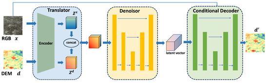
Figure 1.
Structure of LD-DEM.
3.3. Translator
The primary function of the translator is to extract features from the input RGB images and DEM data and transform them into the latent space. We employ the structure of a variational autoencoder (VAE) model. The network architecture is illustrated in Figure 2 and consists of three DownBlock submodules, one ResBlock submodule, one MidBlock submodule, and one GSC submodule.
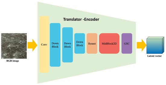
Figure 2.
Structure of translator.
The DownBlock module consists of a padding layer followed by a convolutional layer, which performs downsampling on the input through convolutional operations to extract local features and reduce the spatial dimensions of the image. The MidBlock module includes a ResNet layer, a self-attention layer, and an additional Resnet block. These layers enable nonlinear transformations and enhancements of features. Through these operations, the model can better capture the complex structures and features of the data, thereby improving the quality of the generated images. The GSC module is composed of a GroupNorm layer, a Swish layer, and a convolutional Conv layer. The GroupNorm layer normalizes the input features to enhance the model’s stability. The Swish layer serves as an activation layer, utilizing a smooth activation function expressed as . Compared to the ReLU layer, the Swish layer further enhances the model’s nonlinear expressive capabilities.
Through the functions of the aforementioned modules, the input image is compressed into the latent space, becoming a latent vector with a Gaussian distribution. Due to the fact that high-resolution remote sensing image data under planetary environments are much smaller in scale compared to common image datasets, for instance, datasets used for pre-training VAE encoders, we initialize the parameters of our translator with those of a pre-trained VAE model’s encoder and freeze them to ensure that the translator model has sufficient feature extraction and information transformation capabilities. Since DEM data is single-channel and does not match the existing number of input channels (three channels), we duplicate the DEM data three times to correspond with the dimensions of input channels.
3.4. Denoiser
The denoiser module generates latent vectors for the Digital Elevation Model (DEM) using a UNet architecture, as depicted in Figure 3. This UNet employs a symmetric encoder–decoder structure to process a 6-channel input, combining three channels from the RGB image and three from the DEM, represented as , where H and W denote the initial height and width of the feature map.
Figure 3.
Structure of denoiser.
The encoder comprises three downsampling modules to extract hierarchical features. For each module , the feature map is transformed as follows:
where denotes the learnable parameters (weights and biases) of the module. The first two modules () adopt the standard DownBlock2D structure, each containing two residual blocks (ResNetBlock), defined as follows:
where is a nonlinear activation (e.g., ReLU) and denotes a 3 × 3 convolution with stride 1. These modules apply max pooling to halve the spatial dimensions:
yielding feature maps of resolutions 64 × 64 () and 32 × 32 () for , respectively. The third module () employs the AttnDownBlock2D structure, incorporating a spatial attention mechanism. The attention-weighted feature map is computed as follows:
where applies spatial attention by computing attention scores via
and modulates the feature map as . This module reduces the resolution to 16 × 16 and increases the channel count to .
This encoder design effectively compresses the input into a compact latent representation, capturing multi-scale features for subsequent decoding and DEM generation.
The decoder of the denoiser module reconstructs the latent representation to the original resolution through a three-stage upsampling process, leveraging skip connections to integrate multi-scale features from the encoder. The input to the decoder is the bottleneck feature map from the encoder.
In the first stage, the AttnUpBlock2D module applies a spatial attention mechanism to enhance feature representation, combined with a skip connection from the encoder’s corresponding layer (). The attention-weighted feature map is computed as follows:
where denotes the attention scores and are learnable weights for query and key projections. The modulated feature map is . The skip connection concatenates with the encoder feature map and sends it to , yielding . This is followed by upsampling via trilinear interpolation and convolution:
producing . In the subsequent stages (), UpBlock2D modules upsample the feature maps using
where is the skip-connected feature map from the encoder at matching resolution ( for , for ). This results in and . The final output layer maps the feature map to the original resolution and channel count:
yielding the output . The attention mechanism is applied solely at the 16 × 16 bottleneck to balance computational efficiency and expressive power, while skip connections facilitate the fusion of multi-scale features, enhancing the quality of the reconstructed DEM latent vectors.
3.5. Conditional Decoder
To enable the generated DEM to recover more details from the RGB image during the decoding stage, the RGB image is fed into this module as an auxiliary latent vector to assist in the decoding process of the DEM. The structure of the module is shown in Figure 4.
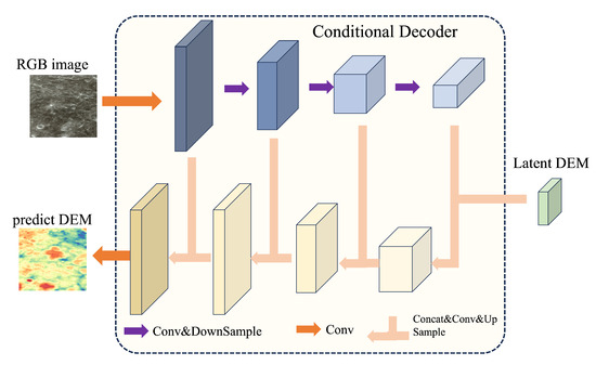
Figure 4.
Structure of decoder.
As shown in Figure 4, the structure of the conditional decoder draws inspiration from the U-Net architecture. Its inputs include the DEM latent vector generated by the denoiser module and the RGB satellite image. The generation process of the conditional decoder is divided into two main steps: downsampling of the RGB image and upsampling of the DEM latent vector.
During the downsampling of the RGB image , the conditional decoder applies three rounds of convolution and max pooling to produce feature maps , where , halving the spatial dimensions (, ) and increasing feature channels (). This generates three hierarchical RGB feature maps . For the upsampling of the DEM latent vector , trilinear interpolation is used to produce , where , doubling spatial dimensions (, ) and reducing channels (). Skip connections concatenate compatible RGB and DEM feature maps as , serving as input to the next upsampling step via . This design effectively fuses RGB and DEM data, enhancing the quality and accuracy of the generated image.
3.6. Model Training
The entire model is trained in a modular fashion. First, we need to complete the training of the denoiser, the training process of which is shown in Figure 5. During the training phase, we select paired RGB images () and DEM images () and feed them into the encoder () to be encoded into latent vectors ( and ). Simultaneously, random noise () is sampled according to different time steps t using a noise generator and added to the latent vector of the DEM () via an ADD operation. After concatenating the noise-added DEM latent vector () with the latent vector of the RGB image () into a combined input (), they are provided as input to the denoiser module () along with the time step t. Inside the denoiser, the feature dimensions are compressed and expanded, and the output is a prediction of the noise (). The output of the denoiser is the predicted noise residual (), and the loss function is
where N is the number of elements in the DEM latent vector, is the i-th true noise value, and is the i-th predicted noise value.
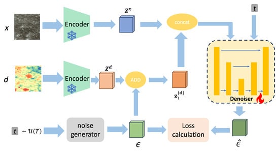
Figure 5.
Training process.
The second step involves training the conditional decoder. First, we use the pre-trained denoiser to generate training data, which means employing this module to produce the corresponding DEM latent vectors for each sample pair in the training set, as shown in Figure 6. During the generation process, we iteratively denoise the initial standard Gaussian noise. The parameters of the denoiser remain unchanged throughout the generation of DEM latent vectors. Since the DDPM noise sampler relies on a Markov process and cannot generate high-quality results across time steps, we instead use the DDIM noise sampler during the generation process. Once a sufficient number of DEM latent vector samples have been generated, we proceed to train the conditional decoder with the aforementioned latent vectors and the ground-truth DEMs. To effectively update the model parameters, we employ the Mean Absolute Error (MAE) loss to enhance the pixel-level accuracy of DEM generation, which is defined as
where is the i-th true value in the DEM and is the i-th predicted value in the generated DEM.
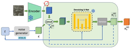
Figure 6.
DEM latent vector generation process.
In the inference process, the RGB image is used as input and encoded into the latent vector by the encoder module and is then concatenated with the noise. Next, the denoiser module iteratively denoises the noise-added latent vector to generate the DEM latent vector. This step is identical to the method used for generating DEM latent vectors during the model training phase. After the DEM latent vector is generated, the conditional decoder decodes the DEM latent vector to obtain the predicted DEM. The inference process of the model can be summarized in Algorithm 1.
| Algorithm 1. Inference process | |
|
|
4. Experiment and Results
In this section, we first introduce the data sources and preprocessing methods for algorithm validation, the parameter settings for the experiments, and the selection of evaluation metrics. Subsequently, through quantitative and visual analyses, we compare the performance of our proposed algorithm with that of the baseline algorithms.
4.1. Experimental Settings and Environment
4.1.1. Dataset
We constructed a dataset using the satellite images and DEMs of Mars provided by NASA [42] and the Lunar and Planetary Data Release System [43], as shown in Figure 7. The images used in this work are created from data assembled by the Lunar Reconnaissance Orbiter camera and laser altimeter instrument teams. The DEM and satellite images of the planetary surfaces both have a resolution of 463 m/pixel, but their dimensions are 27,360 × 13,680 and 23,040 × 11,520, respectively. To match the resolution of the DEM, the RGB satellite images were scaled to ensure pixel alignment. In addition to unifying pixel resolution, the DEM elevation values were normalized to a range of to 15 m to account for the large differences in terrain height across different planets, thereby enhancing the generalizability of our algorithm. RGB satellite images and DEMs near polar regions, which exhibited significant deformation due to scaling and stretching, were excluded from the dataset to ensure suitability for model training and testing.
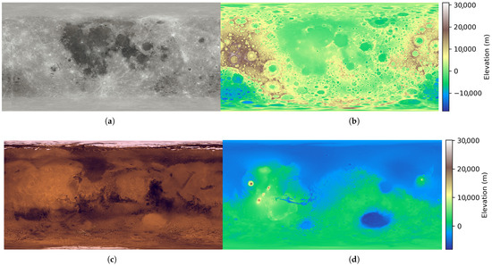
Figure 7.
(a) RGB data of the lunar surface and (b) DEM data of the lunar surface; (c,d) are the RGB data and DEM data of the Mars, respectively.
After alignment, the RGB images and corresponding DEM data were further cropped into image patches with a resolution of 512 × 512 pixels, as shown in Figure 8a,b. The grayscale range of the RGB satellite images is 0–255, while the DEM data range from m to 10 m, which is scaled to the interval of 0–255 for grayscale visualization, as shown in Figure 8c,d. Comparisons between the RGB images, DEM images, and three-dimensional visualizations of the corresponding terrains reveal that the processed DEM images can clearly represent topographic features. However, due to the influence of lighting and viewing angles, shadows and overexposure may appear in the RGB satellite images, which can prevent them from fully and accurately providing information on topographic features. This presents a significant challenge to the model’s ability to extract features and learn the data distribution.
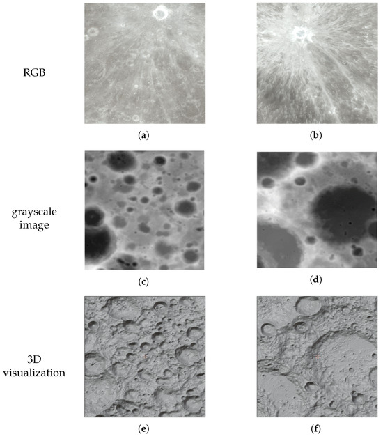
Figure 8.
Cropped RGB image. (a,b) are RGB patches, (c,d) are grayscale images, and (e,f) are corresponding 3D visualizations.
Ultimately, we obtained the planetary dataset following the aforementioned processing steps. The dataset comprises a total of 15,412 samples, with 80% allocated for training and 20% reserved for testing, as shown in Table 1.

Table 1.
Composition of the planetary dataset, including training and testing samples for the Moon and Mars.
4.1.2. Latent Vector Data Generation
To train the conditional decoder, we first trained the denoiser using the planetary dataset. After training, we generated corresponding DEM latent vectors for each sample in the training set to construct the training dataset for the conditional decoder. Specifically, for each sample in the planetary dataset, we generated the predicted DEM latent vector by performing 50 iterations of denoising on randomly initialized Gaussian noise. Since the denoiser is designed to denoise randomly initialized standard Gaussian noise, different initial noise inputs may lead to different denoising outcomes. Therefore, we selected 2846 samples at random and performed iterative denoising from five different initial noise inputs for each sample, resulting in five distinct DEM latent vectors per sample. This approach enhanced the robustness of the conditional decoder. In total, we obtained 14,230 DEM latent vectors from these samples. For the remaining samples, we generated a single DEM latent vector per sample, amounting to 9818 samples.
Additionally, to further expand the dataset, we incorporated DEM latent vectors directly encoded by the encoder into the training samples for the conditional decoder. Through this method, we ultimately obtained a total of 36,712 latent vector–DEM training pairs. This diverse approach to obtaining training samples ensured that the conditional decoder could adapt to different initial noise conditions, thereby improving the model’s generalizability and practicality.
4.1.3. Environment
Our algorithm was implemented on an Ubuntu 20.04 operating system, equipped an NVIDIA A40 (48 G) GPU. During the training of the denoiser, we employed a DDPM noise scheduler with 1000 diffusion steps and used the AdamW optimizer with a learning rate of 1 × 10. The batch size was set to 16, and the entire training process lasted for 10 epochs. For generating the training dataset of the conditional decoder and conducting inference, we used the DDIM noise scheduler with 50 sampling steps. During the training of the conditional decoder, we utilized the AdamW optimizer with a learning rate of 1 × 10. The batch size was set to 8, and the training lasted for 5 epochs.
4.1.4. Evaluation Metrics
To comprehensively evaluate the effectiveness of our method, we conducted assessments from two perspectives: objective metrics and subjective visual inspection.
We employed several evaluation metrics to quantify the reconstruction error. These metrics include the Mean Absolute Error (MAE) and Root Mean Squared Error (RMSE), which are calculated as follows:
where is the i-th predicted value, is the i-th ground-truth value, and N is the total number of pixels.
For subjective evaluation, we primarily compared the visualized predicted DEMs with the ground-truth DEMs to assess the quality of the reconstruction.
4.2. Results and Analysis
Table 2 presents the performance comparison between our method and the two baselines, and the best results are shown in bold. The experimental results show that our proposed method outperforms the Pix2pix algorithm on both the lunar and Martian datasets. Specifically, on the lunar dataset, our method achieved improvements of 37.51% and 28.72% in Mean Absolute Error (MAE) and Root Mean Squared Error (RMSE), respectively. On the Martian dataset, our method demonstrated performance enhancements of 26.92% and 17.67% in MAE and RMSE, respectively, compared to the Pix2pix algorithm. These improvements can be attributed to two main factors. First, the iterative denoising approach of the diffusion models allows for finer control over DEM generation compared to generative adversarial networks (GANs). Second, diffusion models avoid mode collapse, a common issue in GAN training, by progressively learning the data distribution, resulting in higher-quality generations.
Table 2.
Comparison.
Compared to the VAE-LD algorithm, our proposed LD–DEM algorithm achieved improvements of 17.8% and 17.03% in MAE and RMSE, respectively. On the Mars dataset, the performance enhancements were 20.49% and 20.01% in MAE and RMSE, respectively. These improvements indicate that the conditional decoder proposed in this study can effectively integrate information from RGB satellite images. When decoding DEM latent vectors, the provided RGB satellite images offer additional information for DEM reconstruction.
We utilized the BlenderGIS plugin in Blender for three-dimensional visualization analysis and the Matplotlib (version 1.3.0) library in Python (version 3.13) for two-dimensional visualization analysis, as shown in Figure 9. Through these diverse visualization methods, we were able to conduct subjective analyses from different perspectives by visually inspecting the results.
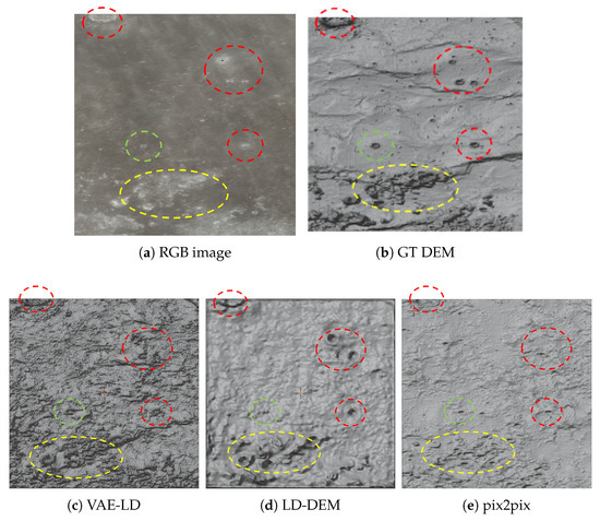
Figure 9.
Comparison of 3D visualization; marked regions are highlighted with red, green, and yellow circles.
As shown in Figure 9, we first visualized the DEM prediction results for the lunar RGB satellite images with small features from the test dataset. It can be observed that the small features marked by red circles are well detected and generated by LD–DEM. However, for the terrain marked by green circles, none of the three algorithms were able to effectively reconstruct it. For the large-scale complex terrain marked by yellow circles, LD-DEM performed better than the other models in terms of terrain reconstruction, while the results of VAE-LD still contained considerable noise.
As shown in Figure 10, through two-dimensional visualization of the generated DEMs, it can be intuitively seen that the DEMs generated by LD-DEM have smaller overall deviations and can better capture the details in the RGB satellite images. Compared with the RGB satellite images, the results predicted by Pix2pix are more affected by lighting and lack sufficient reconstruction of terrain details. Although VAE-LD performs better in reconstructing terrain details, its overall prediction is inferior to that of LD-DEM due to the lack of global image information during decoding.
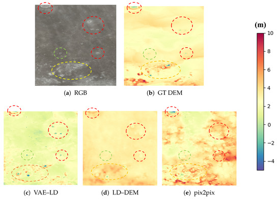
Figure 10.
Comparison of DEM predictions with marked regions (red, green, and yellow circles) and height colorbar (m).
Figure 11 and Figure 12 illustrate the DEM reconstruction results of different models for lunar RGB satellite images containing shadowed areas. DEM generation under such conditions is challenging because shadows can obscure the true topographic features, making it difficult to directly identify terrain characteristics from RGB images. As shown in the figure, in the areas marked by red circles, LD-DEM is able to accurately reconstruct the true terrain despite the difficulty in discerning terrain details from the RGB satellite images. This demonstrates that LD-DEM possesses strong robustness and efficient terrain feature extraction capabilities when dealing with lighting variations and shadow occlusions. By comparing the three-dimensional visualizations of the DEM terrain, we can clearly observe the high consistency between the terrain reconstructed by our proposed LD-DEM and the true terrain.
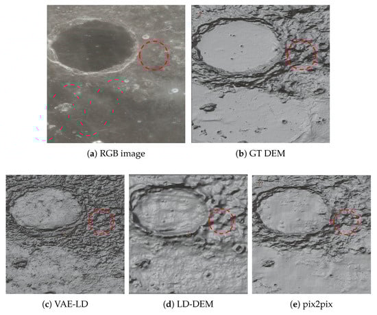
Figure 11.
Three-dimensional visualization of shadowed areas.
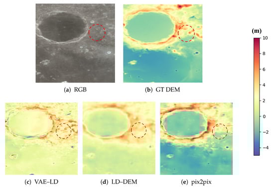
Figure 12.
DEM comparison of shadowed areas on the moon.
For the prediction of flat terrain, the results shown in Figure 11 indicate that the Pix2pix model performs slightly better than LD-DEM. This is because the Pix2pix model is more stable when processing relatively uniform or less variable terrain, while LD-DEM over-interprets minor variations in the data. The two-dimensional visualization in Figure 12 also corroborates our analysis, showing that the prediction results of Pix2pix are generally superior to those of LD-DEM and VAE-LD.
Figure 13 and Figure 14 illustrate the effects of generating Martian topography using Mars RGB satellite imagery, comparing the performance of the LD-DEM and VAE-LD models. It can be observed from the figures that the terrain generated by LD-DEM is smoother and successfully reconstructs some prominent topographical features, such as valleys and craters. This indicates that LD-DEM can effectively capture and reconstruct key topographical structures when processing Martian topographical data. The smooth terrain generation demonstrates that the model is capable of integrating information from the input data and reducing unnecessary noise, thereby producing a more accurate and realistic visual representation of the terrain. In contrast, the terrain generated by VAE-LD contains more noise and fails to reconstruct some key topographical features.
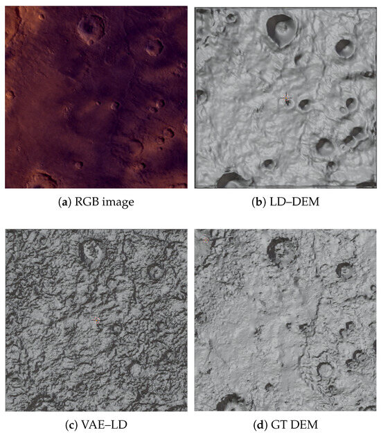
Figure 13.
Three-dimensional visualization of Mars’ DEM.

Figure 14.
DEM comparison on Mars.
Ablation Experiments
In this subsection, ablation experiments are conducted to investigate the effects of LD-DEM and VAE-LD in decoding DEM latent vectors. To explore the effectiveness and robustness of the conditional decoder, we performed comparative experiments with 50 iterations of denoising and 100 iterations of denoising, respectively. The results are shown in Table 3. The arrow means that the lower, the better for the metrics, and numbers in bold mean the best results. As can be seen, the errors generated by the proposed LD-DEM decoding are smaller than those of the comparison algorithms in both 50 and 100 iterations of denoising. Moreover, the visual analysis confirms that the observed noise is indeed less, which demonstrates the effectiveness of the conditional decoder module in the proposed LD-DEM. When decoding the DEM latent vectors with 100 iterations of denoising, neither VAE-LD nor LD-DEM shows a significant improvement in metrics. This suggests that the DEM latent vectors after 50 iterations of denoising are sufficient to reflect the main features of the terrain.
Table 3.
Precision comparison of different decoders.
The 3D visualization results for different iterations are shown in Figure 15. The terrain marked by the red dashed circle exhibits indistinct features in the RGB satellite imagery. However, both VAE-LD and LD-DEM partially reconstruct this terrain in the DEM generated after 50 iterations of denoising. After 100 iterations of denoising, both algorithms introduce errors in reconstructing this terrain, yet they achieve better restoration of the prominent features in the RGB imagery, indicating that LD-DEM progressively enhances RGB image constraint control during the denoising process.
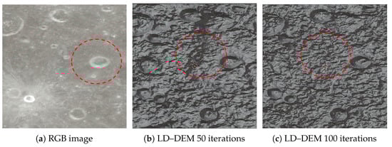
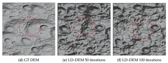
Figure 15.
Three-dimensional visualization results for different iterations of various algorithms.
5. Summary
This study proposes an algorithm named LD-DEM for generating DEMs from single RGB satellite images. By leveraging a diffusion-based generative model for iterative denoising and introducing a conditional decoder to integrate RGB image information during the decoding process, our method achieves superior performance compared to existing algorithms. Unlike generative adversarial networks, our proposed algorithm exhibits greater stability during training and faster model convergence. Ablation experiments confirm that the conditional decoder effectively reconstructs DEM details and achieves higher accuracy when decoding DEM latent vectors.
Although the current algorithm generates high-quality DEMs, geographic information such as latitude and longitude data remains underutilized. Furthermore, for planets with distinct surface compositions, such as ice, variations in surface albedo may significantly impact model performance, necessitating the inclusion of albedo as a critical parameter to enhance generalizability. However, the current lack of sufficient data for planets with non-rocky surfaces limits our ability to conduct comprehensive generalization experiments. We plan to address this in future work by incorporating additional data from such planetary surfaces to further validate and broaden the applicability of our model.
Author Contributions
Conceptualization, L.S. and H.Z.; methodology, L.S.; software, H.Z.; validation, H.Z.; formal analysis, H.Z.; investigation, H.Z.; resources, L.S. and L.Y.; data curation, L.S. and H.Z.; writing—original draft preparation, L.S.; writing—review and editing, L.S. and D.Z. (Dengyang Zhao); visualization, H.Z.; supervision, L.Y. and D.Z. (Dongping Zhang); funding, L.Y. All authors have read and agreed to the published version of the manuscript.
Funding
This work was supported by the National Natural Science Foundation of China under Grant 52372423, “Pioneer” and “Leading Goose” R&D Program of Zhejiang (grant number 2024C01028), Key R&D projects in Zhejiang Province [No. 2024C01102], and Key R&D projects in Ningbo [No. 2024Z114].
Data Availability Statement
The original contributions presented in the study are included in the article, further inquiries can be directed to the corresponding author.
Conflicts of Interest
The authors declare no conflicts of interest.
Abbreviations
The following abbreviations are used in this manuscript:
| DEM | Digital Elevation Model |
| CNNs | Convolutional Neural Networks |
| GANs | Generative Adversarial Networks |
| LD–DEM | Latent Diffusion-based DEM |
| DDPM | Denoising Diffusion Probabilistic Model |
| VAE | Variational Autoencoder |
| DDIM | Denoising Diffusion Implicit Model |
References
- Tong, X.; Feng, Y.; Ye, Z. Illumination Robust Landing Point Visual Localization for Lunar Lander With High-Resolution Map Generation. IEEE J. Sel. Top. Appl. Earth Obs. Remote Sens. 2024, 17, 1577–1591. [Google Scholar] [CrossRef]
- Cao, W.; Xiao, Z.; Luo, F.; Ma, Y.; Ouyang, H.; Xu, R. Emplacement mechanism of ponded light plains on the moon: Insight from topography roughness. Icarus 2024, 415, 116071. [Google Scholar] [CrossRef]
- Elias, M.; Isfort, S.; Eltner, A. UAS Photogrammetry for Precise Digital Elevation Models of Complex Topography: A Strategy Guide. ISPRS Ann. Photogramm. Remote Sens. Spat. Inf. Sci. 2024, 10, 57–64. [Google Scholar] [CrossRef]
- Smith, D.E.; Zuber, M.T.; Jackson, G.B.; Cavanaugh, J.F.; Neumann, G.A.; Riris, H.; Sun, X.; Zellar, R.S.; Coltharp, C.; Connelly, J.; et al. The lunar orbiter laser altimeter investigation on the lunar reconnaissance orbiter mission. Space Sci. Rev. 2010, 150, 209–241. [Google Scholar] [CrossRef]
- Uwe, L. Laserscanning For DEM Generation. WIT Trans. Inf. Commun. Technol. 1998, 21, 7. [Google Scholar]
- Escobar Villanueva, J.R.; Iglesias Martinez, L.; Perez Montiel, J.I. DEM generation from fixed-wing UAV imaging and LiDAR-derived ground control points for flood estimations. Sensors 2019, 19, 3205. [Google Scholar] [CrossRef] [PubMed]
- Feng, S.; Lin, Y.; Wang, Y. DEM generation with a scale factor using multi-aspect SAR imagery applying radargrammetry. Remote Sens. 2020, 12, 556. [Google Scholar] [CrossRef]
- Sefercik, U.G. Comparison of DEM accuracies generated by various methods. In Proceedings of the 3rd International Conference on Recent Advances in Space Technologies, Istanbul, Turkey, 14–16 June 2007; pp. 379–382. [Google Scholar]
- Tao, L.; Zhong, X.; Wu, T. DEM Generation with High-Resolution Repeat-Pass Interferometry for Airborne Squinted SAR Acquisitions. In Proceedings of the 6th Asia-Pacific Conference on Synthetic Aperture Radar (APSAR), Xiamen, China, 26–29 November 2019; pp. 1–5. [Google Scholar]
- Daying, Q.; Feitao, R.; Xiaofeng, W.; Mengdao, X.; Ning, J.; Dongping, Z. WVD-GAN: A Wigner-Ville distribution enhancement method based on generative adversarial network. IET Radar Sonar Navig. 2024, 18, 849–865. [Google Scholar]
- Beckham, C.; Pal, C. A Step Towards Procedural Terrain Generation with GANs. arXiv 2017, arXiv:1707.03383. [Google Scholar] [CrossRef]
- Yilin, Z.; Lingmin, H.; Xiangping, W.; Chen, P. Self-training and Multi-level Adversarial Network for Domain Adaptive Remote Sensing Image Segmentation. Neural Process. Lett. 2021, 55, 10197–10216. [Google Scholar]
- Voulgaris, G.; Mademlis, I.; Pitas, I. Procedural terrain generation using generative adversarial networks. In Proceedings of the 29th European Signal Processing Conference (EUSIPCO), Dublin, Ireland, 23–27 August 2021; pp. 686–690. [Google Scholar]
- Demiray, B.Z.; Sit, M.; Demir, I. D-SRGAN: DEM Super-Resolution with Generative Adversarial Networks. SN Comput. Sci. 2021, 2, 48. [Google Scholar] [CrossRef]
- Chen, Z.; Wu, B.; Liu, W.C. Mars3DNet: CNN-based high-resolution 3D reconstruction of the Martian surface from single images. Remote Sens. 2021, 13, 839. [Google Scholar] [CrossRef]
- Yang, L.; Zhu, Z.; Sun, L. Global attention-based DEM: A planet surface digital elevation model-generation method combined with a global attention mechanism. Aerospace 2024, 11, 529. [Google Scholar] [CrossRef]
- Chen, H.; Gläser, P.; Hu, X. ELunarDTMNet: Efficient reconstruction of high-resolution lunar DTM from single-view orbiter images. IEEE Trans. Geosci. Remote Sens. 2024, 62, 1–12. [Google Scholar] [CrossRef]
- Zhou, A.; Chen, Y.; Wilson, J.P. A multi-terrain feature-based deep convolutional neural network for constructing super-resolution DEMs. Int. J. Appl. Earth Obs. Geoinf. 2023, 120, 103338. [Google Scholar] [CrossRef]
- Luo, S.; Tan, Y.; Huang, S.; Li, J.; Zhao, H. Latent Consistency Models: Synthesizing High-Resolution Images with Few-Step Inference. Comput. Vis. Pattern Recognit. 2024, 8, 1–15. [Google Scholar]
- Zhu, M.; Xu, Z.; Wang, X.; Chen, Y.; Li, H.; Zhang, Q. LatentExplainer: Explaining Latent Representations in Deep Generative Models with Multimodal Large Language Models. arXiv 2025, arXiv:2406.14862. [Google Scholar]
- Pan, Y.; Zhang, L.; Wang, H. Style-Guided Text-to-Image Diffusion Models with Reference Image Support. Artif. Intell. Rev. 2023, 56, 12345–12360. [Google Scholar]
- Rombach, R.; Blattmann, A.; Lorenz, D. High-resolution image synthesis with latent diffusion models. In Proceedings of the IEEE/CVF Conference on Computer Vision and Pattern Recognition, New Orleans, LA, USA, 19–24 June 2022; pp. 10684–10695. [Google Scholar]
- Saxena, S.; Kar, A.; Norouzi, M. Monocular Depth Estimation Using Diffusion Models. arXiv 2017, arXiv:2302.14816. [Google Scholar]
- Duan, Y.; Guo, X.; Zhu, Z. Diffusiondepth: Diffusion denoising approach for monocular depth estimation. In Proceedings of the European Conference on Computer Vision, Milan, Italy, 29 September–4 October 2024; pp. 432–449. [Google Scholar]
- Patni, S.; Agarwal, A.; Arora, C. Ecodepth: Effective conditioning of diffusion models for monocular depth estimation. In Proceedings of the IEEE/CVF Conference on Computer Vision and Pattern Recognition, Seattle, WA, USA, 17–21 June 2024; pp. 28285–28295. [Google Scholar]
- Tosi, F.; Ramirez, P.Z.; Poggi, M. Diffusion models for monocular depth estimation: Overcoming challenging conditions. In Proceedings of the European Conference on Computer Vision, Milan, Italy, 29 September–4 October 2024; pp. 236–257. [Google Scholar]
- Chen, Y.; Yu, L.; Wang, Z. DiffDRNet: A Latent Diffusion Model-Based Method for Depth Completion. In Proceedings of the 10th International Conference on Systems and Informatics (ICSAI), Shanghai, China, 13–15 November 2024; pp. 1–6. [Google Scholar]
- Hu, Z.; Hu, K.; Mo, C. Terrain Diffusion Network: Climatic-Aware Terrain Generation with Geological Sketch Guidance. In Proceedings of the AAAI Conference on Artificial Intelligence, Vancouver, BC, Canada, 20–27 February 2024; pp. 12565–12573. [Google Scholar]
- Panagiotou, E.; Chochlakis, G.; Grammatikopoulos, L. Generating Elevation Surface from a Single RGB Remotely Sensed Image Using Deep Learning. Remote Sens. 2020, 12, 2002. [Google Scholar] [CrossRef]
- Chen, H.; Hu, X.; Oberst, J. Pixel-resolution DTM generation for the lunar surface based on a combined deep learning and shape-from-shading (SFS) approach. ISPRS Ann. Photogramm. Remote Sens. Spat. Inf. Sci. 2022, 3, 511–516. [Google Scholar] [CrossRef]
- Bertone, S.; Barker, M.K.; Mazarico, E. Large-Scale Elevation Models to Support Optical Navigation to the Lunar Surface. 2023. Available online: https://zenodo.org/records/10258683 (accessed on 21 July 2025.).
- Wang, Y.; Jin, S.; Yang, Z. TTSR: A transformer-based topography neural network for digital elevation model super-resolution. IEEE Trans. Geosci. Remote Sens. 2024, 62, 1–19. [Google Scholar] [CrossRef]
- Al-Fugara, A.; Almomani, M.H.; Zitar, R.A. Enhanced deep learning network for accurate digital elevation model generation from LiDAR data. Autom. Constr. 2024, 167, 105708. [Google Scholar] [CrossRef]
- Paul, S.; Ashutosh, G.A. Regularized Adversarial Network for Image Guided DEM Super-resolution Using Frequency Selective Hybrid Graph Transformer. In International Conference on Pattern Recognition; Springer: Cham, Switzerland, 2025; pp. 389–405. [Google Scholar]
- Ramos, N.; Santos, P.; Dias, J. Dual critic conditional Wasserstein GAN for height-map generation. In Proceedings of the 18th International Conference on the Foundations of Digital Games, Lisbon, Portugal, 11–14 April 2023; pp. 1–4. [Google Scholar]
- Huang, Y.L.; Yuan, X.F. StyleTerrain: A novel disentangled generative model for controllable high-quality procedural terrain generation. Comput. Graph. 2023, 116, 373–382. [Google Scholar] [CrossRef]
- Zhao, Y.; Wu, B.; Kong, G. Generating high-resolution DEMs in mountainous regions using ICESat-2/ATLAS photons. Int. J. Appl. Earth Obs. Geoinf. 2025, 138, 104461. [Google Scholar] [CrossRef]
- Ho, J.; Jain, A.; Abbeel, P. Denoising diffusion probabilistic models. Adv. Neural Inf. Process. Syst. 2020, 33, 6840–6851. [Google Scholar]
- Zhang, D.; Li, J.; Chen, Z.; Zou, Y. Efficient image generation with Contour Wavelet Diffusion. Comput. Graph. 2024, 124, 839. [Google Scholar] [CrossRef]
- De Groot, S.R.; Mazur, P. Non-Equilibrium Thermodynamics, 1st ed.; Courier Corporation: Mineola, NY, USA, 2013. [Google Scholar]
- Blumenthal, R.M.; Getoor, R.K. Markov Processes and Potential Theory, 1st ed.; Courier Corporation: Mineola, NY, USA, 2007. [Google Scholar]
- NASA. Available online: https://svs.gsfc.nasa.gov/ (accessed on 18 June 2025).
- Lunar and Planetary Data Release System. Available online: http://moon.bao.ac.cn (accessed on 18 June 2025).
Disclaimer/Publisher’s Note: The statements, opinions and data contained in all publications are solely those of the individual author(s) and contributor(s) and not of MDPI and/or the editor(s). MDPI and/or the editor(s) disclaim responsibility for any injury to people or property resulting from any ideas, methods, instructions or products referred to in the content. |
© 2025 by the authors. Licensee MDPI, Basel, Switzerland. This article is an open access article distributed under the terms and conditions of the Creative Commons Attribution (CC BY) license (https://creativecommons.org/licenses/by/4.0/).