A New Methodological Approach to the Reachability Analysis of Aerodynamic Interceptors

Abstract

Advanced air defense methods are essential to address the growing complexity of aerial threats. The increasing number of targets necessitates better defensive coordination, and a promising strategy involves the use of interceptors together to protect a specific area. This task fundamentally depends on accurately predicting their kinematic envelopes, or reachable sets. This paper presents a novel approach to determine the boundaries of reachable sets for aerodynamic interceptors, accounting for energy loss from drag, energy gain from thrust, variable acceleration limits, and autopilot dynamics. The devised numerical method approximates reachable sets for nonlinear problems using a constrained model predictive programming concept. Results demonstrate that explicitly accounting for input constraints, such as acceleration limits, significantly impacts the shape and area of the reachable boundaries. Furthermore, a sensitivity analysis was conducted to demonstrate the impact of parameter variations on the reachable set. Revealing the reachable set’s sensitivity to variations in thrust and drag coefficients, this analysis serves as a framework for considering parameter uncertainty and enables the evaluation of these effects prior to embedding the reachability boundaries into an offline database for guidance applications. The resulting boundaries, representing minimum and maximum ranges for various initial parameters, can be stored offline, allowing interceptors to estimate their own or allied platforms’ kinematic capabilities for cooperative strategies.

1. Introduction

Today’s air defense systems are facing greater challenges, driven by an increase in coordinated attacks that use multiple threats with different capabilities. These complex engagement scenarios, combined with uncertainties in target states and unpredictable maneuvers, strain traditional one-to-one interceptor allocation strategies and create a need for more advanced air defense capabilities. Therefore, strategies that leverage the full kinematic potential of aerodynamic interceptors are important for mission success. The midcourse guidance phase, in particular, is critical for medium and long-range interceptors due to its extended duration.

To understand the context of this challenge, it is useful to review the existing literature. The development of guidance strategies has a rich history, with many approaches derived from proportional navigation (PN) and optimal control methodologies. While PN-based methods are widely used, they often do not evaluate potential target maneuvers. Optimal control-based laws [1,2,3] typically focus on objectives such as minimizing energy loss but often neglect to confirm if a feasible trajectory to the desired destination exists given the available control inputs. To address these gaps and enhance robustness, reachability-based guidance [4] has been proposed as a modern alternative. These strategies utilize the concept of a “reachable set”—the collection of all states a system can attain from a given initial condition under all admissible control inputs over a specified time horizon. Reachability has proven valuable in domains such as dynamic coverage and area defense. Although the full system state may include attributes like velocity and orientation, this work focuses specifically on reachable positions. The process of computing these sets is known as reachability analysis.

The effectiveness of these advanced strategies, however, is entirely dependent on the accurate and realistic computation of the reachable set itself. Methodologies for computing reachable sets are diverse, generally balancing solution accuracy against computational requirements. For the nonlinear systems addressed in this work, three main categories of techniques are prevalent:

Level Set Methods [5,6]: These methods solve time-dependent partial differential equations (PDEs) to define the boundary of the reachable set. While advantageous for capturing the full boundary, this approach can be computationally complex, limiting its application to lower-dimensional systems.

Approximate Geometric Methods: This class of techniques approximates the reachable set using predefined convex geometries such as ellipsoids [7] or zonotopes [8]. These methods are well suited for linear systems but are less applicable to the nonconvex sets typical of nonlinear systems. A significant drawback is the computational burden of growing the geometric set at each time step, often requiring cumbersome Minkowski sum [9] operations that can lead to the “wrapping effect”—an accumulation of errors that causes over-approximation of the set.

Optimization-Based Methods: These techniques formulate the computation of reachable sets as an optimization problem. For general nonlinear systems, a common approach [10,11] involves discretizing a region of the state space into a grid and solving an optimal control problem for each point to determine if it is reachable. This method utilizes grids to cover the region of interest, and the distance function to the reachable set is evaluated at each grid point. The primary benefit is the elimination of complex set operations, but its main limitation is the “curse of dimensionality,” as the number of grid points required to cover the state space—and thus the overall computational cost—grows exponentially with the system’s dimension.

This review reveals a need for a method that can compute accurate reachable sets for high-fidelity, nonlinear systems without the drawbacks of geometric approximations or exhaustive state-space discretization. This paper addresses this gap by proposing a novel framework for computing the reachable set boundaries for an aerodynamic interceptor. An input-constrained suboptimal midcourse guidance algorithm founded on the principles of model predictive static programming (MPSP) is developed and applied. The algorithm is designed to be energy-efficient while strictly enforcing input constraints based on the vehicle’s state-dependent acceleration limits, which are handled using Hildreth’s quadratic programming procedure.

A primary contribution of this research is a new computational method for determining the reachable set boundaries of nonlinear systems with state-dependent input constraints. This approach directly circumvents the fundamental limitations of traditional techniques. Instead of relying on computationally intensive grid-based discretization or geometric set operations, the proposed approach uses directional search to identify the minimum and maximum range boundaries. This technique probes for the boundary along predefined search directions, solving the nonlinear optimal control problem only for candidate points on the envelope’s edge, and hence avoids discretizing the entire state space volume. The algorithm’s efficiency stems from two key features. First, the search along each direction terminates as soon as an unreachable point is found, which identifies the boundary without testing unnecessary points further away. Second, it accelerates the process by reusing optimal control information, where the solution for the previous reachable point serves as a high-quality initial guess for the next point’s optimization problem.

Furthermore, a comparative analysis is included to demonstrate the significant impact of input constraints on the interceptor’s kinematic capabilities, along with a sensitivity analysis to evaluate how variations in system parameters affect the shape of the reachable sets. The resulting framework provides a tool for generating high-fidelity reachable sets, which can be stored in an offline database to support advanced cooperative guidance strategies.

The paper is organized as follows: In Section 2, the nonlinear interceptor system model is summarized. In Section 3, a formal mathematical statement of the problem is provided. In Section 4, the constrained model predictive approach is explained. Additionally, the reachability concept and the reachable set computation procedure are summarized. In Section 5, several reachability boundaries are demonstrated, and a sensitivity analysis is conducted to assess the influence of system parameters. Finally, some conclusions are drawn.

2. Modeling

To analyze the reachable set, a mathematical model capturing the interceptor’s flight dynamics is required. This study employs a point mass model that accounts for non-ideal responses and physical effects. The model is built on the following specific characteristics and assumptions:

Propulsion: The interceptor is powered by a two-pulse rocket motor.

Mass: The interceptor’s mass is variable and decreasing as propellant is expelled, which is directly coupled to the thrust profile.

Autopilot: The interceptor’s lateral acceleration response is not instantaneous. A first-order autopilot model with a time constant τ is used to model the lateral acceleration response dynamics due to lateral acceleration commands.

Environment: The model incorporates a standard atmosphere model where the effect of altitude on atmospheric conditions is reflected by dynamic pressure. The effect of wind on lateral dynamics is assumed to be compensated for by the autopilot. However, the effect of wind on longitudinal dynamics is not taken into account.

Aerodynamics: Total drag is calculated by combining two distinct components: a base drag that changes with the interceptor’s velocity and an additional drag penalty incurred from maneuvering. The energy loss of the interceptor due to lateral acceleration drag and base drag is incorporated into the drag coefficient, which is expressed as follows [12,13]:

$$C_X\left({a_M}_y^W,{a_M}_z^W,V_M\right)={C_X}_0\left(V_M\right)+{C_X}_a\left(V_M\right)\sqrt{{a_{M_y}^W}^2+{a_{M_z}^W}^2}$$

(1)

$\sqrt{{a_{M_y}^W}^2+{a_{M_z}^W}^2}$ term increases the drag coefficient due to the magnitude of lateral accelerations. $C_{X_0}\left(V_M\right)$ is the velocity-dependent base drag coefficient. $C_{X_a}\left(V_M\right)$ defines the increase in drag coefficient due to lateral accelerations.

The coordinate axes of the inertial frame ${\mathcal{F}}_I$ and wind frame ${\mathcal{F}}_W$ are shown in Figure 1 [12,13]. The velocity vector ${\overrightarrow{V}}_M$ is in the direction of ${\overrightarrow{u}}_1^W$.

The non-ideal interceptor model is represented as follows [12,13]:

$$\begin{array}{l}\overline{x}\left(k+1\right)=\left[\begin{array}{c}{R_M}_x\left(k+1\right)\\ {R_M}_y\left(k+1\right)\\ {R_M}_z\left(k+1\right)\\ V_M\left(k+1\right)\\ \alpha \left(k+1\right)\\ \beta \left(k+1\right)\\ {a_M}_y^W(k+1)\\ {a_M}_z^W(k+1)\end{array}\right]\\ =\left[\begin{array}{c}{R_M}_x\left(k\right)+V_M\left(k\right)\mathit{cos}\left(\beta \left(k\right)\right)\mathit{cos}\left(\alpha \left(k\right)\right)\mathit{\Delta }t\\ {R_M}_y\left(k\right)+V_M\left(k\right)\mathit{cos}\left(\beta \left(k\right)\right)\mathit{sin}\left(\alpha \left(k\right)\right)\mathit{\Delta }t\\ {R_M}_z\left(k\right)-V_M\left(k\right)\mathit{sin}\left(\beta \left(k\right)\right)\mathit{\Delta }t\\ V_M\left(k\right)+{\displaystyle \frac{T-0.5\rho V_M^2{S}_{ref}{C}_X\left({a_M}_y^W\left(k\right),{a_M}_z^W\left(k\right),V_M\left(k\right)\right)}{m}}\mathit{\Delta }t-gsin\left(\beta \left(k\right)\right)\mathit{\Delta }t\\ \alpha \left(k\right)+{\displaystyle \frac{{a_M}_y^W\left(k\right)}{V_M\left(k\right)\mathit{cos}\left(\beta \left(k\right)\right)}}\mathit{\Delta }t\\ \beta \left(k\right)-{\displaystyle \frac{{a_M}_z^W\left(k\right)}{V_M\left(k\right)}}\mathit{\Delta }t\\ {a_M}_y^W\left(k\right)e^{-{\displaystyle \frac{\mathit{\Delta }t}{\tau }}}+{a_M}_{y,c}^W\left(k\right)\left(1-e^{-{\displaystyle \frac{\mathit{\Delta }t}{\tau }}}\right)\\ {a_M}_z^W\left(k\right)e^{-{\displaystyle \frac{\mathit{\Delta }t}{\tau }}}+{a_M}_{z,c}^W\left(k\right)\left(1-e^{-{\displaystyle \frac{\mathit{\Delta }t}{\tau }}}\right)\end{array}\right]\\ =\overline{F}\left(\overline{x}\left(k\right),\overline{u}\left(k\right)\right)=\left[\begin{array}{c}{F}_1\left(\overline{x}\left(k\right),\overline{u}\left(k\right)\right)\\ F_2\left(\overline{x}\left(k\right),\overline{u}\left(k\right)\right)\\ F_3\left(\overline{x}\left(k\right),\overline{u}\left(k\right)\right)\\ F_4\left(\overline{x}\left(k\right),\overline{u}\left(k\right)\right)\\ F_5\left(\overline{x}\left(k\right),\overline{u}\left(k\right)\right)\\ F_6\left(\overline{x}\left(k\right),\overline{u}\left(k\right)\right)\end{array}\right]\end{array}$$

(2)

The input vector is defined as follows:

$$\overline{u}\left(k\right)=\left[\begin{array}{c}{a_M}_{y,c}^W\left(k\right)\\ {a_M}_{z,c}^W\left(k\right)\end{array}\right]$$

(3)

3. Problem Formulation

The core objective of this study is to determine the reachable set of an interceptor vehicle during its midcourse flight phase under bounded control input constraints. The interceptor is modeled as a point-mass system subjected to aerodynamic drag, which is a function of speed and lateral acceleration magnitude. The control input is defined as the lateral acceleration command vector, subject to state-dependent inequality constraints.

The system dynamics in discrete time can be described as in Equation (4):

$$\overline{\mathrm{x}}\left(k+1\right)=\overline{F}\left(\overline{x}\left(k\right),\overline{u}\left(k\right)\right),\overline{\mathrm{x}}\left(0\right)=x_0$$

(4)

$\overline{\mathrm{x}}\left(k\right)\in R^8$ represents the state vector including position, speed, flight path angles, heading angles, and lateral accelerations, as shown in Equation (2). Additionally, $\overline{u}\left(k\right)\in R^2$ denotes the control inputs in terms of lateral acceleration commands. The control inputs are subject to inequality constraints as shown below:

$${\mathit{G}}_{\mathit{k}}{\overline{u}}_k\le {\overline{W}}_k,{\mathit{G}}_{\mathit{k}}=\left[\begin{array}{cc}1& 0\\ -1& 0\\ 0& 1\\ 0& -1\end{array}\right],{\overline{W}}_k=\left[\begin{array}{c}a\left(k\right)\\ a\left(k\right)\\ b\left(k\right)\\ b\left(k\right)\end{array}\right]$$

(5)

where ${\mathit{G}}_{\mathit{k}}$ and ${\overline{W}}_k$ represent the constraints, and $a\left(k\right)$, $b\left(k\right)$ denote the maximum achievable accelerations for lateral axes.

The reachable set $R\left(T|\overline{x}\left(t_0\right),t_0\right)$ at a specific time T for the given initial condition $\overline{x}\left(t_0\right)$ is defined as the set of all terminal positions that can be reached under all admissible control sequences $U$. The mathematical description is shown in Equation (6):

$$\mathcal{R}\left(T|\overline{x}\left(t_0\right),t_0\right)=\left\{\mathit{C}\overline{x}\left(T\right)|\exists \overline{u}\left(.\right)\in {\mathcal{U}}_{{[t}_o,T]}\right\}$$

(6)

where $\mathit{C}\overline{x}\left(T\right)=\left[\begin{array}{c}{R_M}_x\left(T\right)\\ {R_M}_y\left(T\right)\\ {R_M}_z\left(T\right)\end{array}\right]$ is the terminal position vector at the final time $T$, and ${\mathcal{U}}_{\left[t_0,T\right]}$ is the set of all admissible control inputs over $\left[t_0,T\right]$.

The goal of this study is to compute the boundaries of the reachable set $R\left(T|\overline{x}\left(t_0\right),t_0\right)$ while adhering to input constraints and avoiding high-dimensional grid discretization or conservative geometric approximations. To achieve this, we employ a two-level computational approach. First, a directional search algorithm is utilized to determine the minimum and maximum range boundaries by iteratively identifying and testing candidate points along a specified search direction (detailed in Section 4.2 and Section 4.3). Second, for each candidate point, the constrained optimal control problem defined here is solved using a model predictive programming approach to confirm its reachability (detailed in Section 4.1). The results of applying this framework are then demonstrated in Section 5.

4. Methodology

4.1. Input-Constrained Model Predictive Programming

The input-constrained model predictive programming (MPP) approach modifies the initial control input vector to simultaneously meet terminal position constraints and input limitations. For the nonlinear system described, the output is defined as ${\overline{y}}_k$, and the objective is to compute a control input vector ${\overline{u}}_k$ for time steps $k=1,2,\cdots ,\left(N-1\right)$ such that the output at step N matches the desired value ${\overline{y}}_N^d$, while minimizing control effort and satisfying input constraints ${\mathit{G}}_{\mathit{k}}{\overline{u}}_k\le {\overline{W}}_k$, where ${\mathit{G}}_{\mathit{k}}$ and ${\overline{W}}_k$ define the acceleration limits in lateral directions. This approach, which was detailed in [12,13], is briefly summarized in this section, focusing on the input-constrained model predictive programming. The optimization problem is solved using the MPP approach with Hildreth’s procedure for inequality constraints. Linearization of the system around an initial control vector history allows reformulation of the cost function and constraints in terms of variations $d{\overline{u}}_k$, as shown in Equation (7) [14]:

$$J={\displaystyle \frac{1}{2}}\sum _{k=1}^{N-1}{\left({\overline{u}}_k^{*}-d{\overline{u}}_k\right)}^T{\mathit{R}}_{\mathit{k}}\left({\overline{u}}_k^{*}-d{\overline{u}}_k\right)$$

(7)

The equality constraint ensures $d{\overline{y}}_N={\overline{y}}_N^d-{\overline{y}}_N^{*}=0$, and ${\mathit{G}}_{\mathit{k}}\left({\overline{u}}_k^{*}-d{\overline{u}}_k\right)-{\overline{W}}_k\le 0,k=1,2,\cdots ,\left(N-1\right)$. Using Lagrange multipliers, the Hamiltonian function incorporates equality and inequality constraints as shown in Equation (8):

$$\begin{array}{l}{J}^{\mathrm{*}}\left(d{\overline{u}}_k,\overline{\lambda },{\overline{\rho }}_1,{\overline{\rho }}_2,\cdots ,{\overline{\rho }}_{N-1}\right)\\ ={\displaystyle \frac{1}{2}}{\displaystyle \sum _{k=1}^{N-1}}{\left({\overline{u}}_k^{*}-d{\overline{u}}_k\right)}^T{\mathit{R}}_{\mathit{k}}\left({\overline{u}}_k^{*}-d{\overline{u}}_k\right)+{\overline{\lambda }}^T\left(d{\overline{y}}_N-{\displaystyle \sum _{k=1}^{k=N-1}}{\mathit{B}}_{\mathit{k}}d{\overline{u}}_k\right)\\ +\left({\displaystyle \sum _{k=1}^{N-1}}{\overline{\rho }}_k^T\left({\mathit{G}}_{\mathit{k}}\left({\overline{u}}_k^{*}-d{\overline{u}}_k\right)-{\overline{W}}_k\right)\right)\end{array}$$

(8)

where $\overline{\lambda },{\overline{\rho }}_1,{\overline{\rho }}_2,\cdots ,{\overline{\rho }}_{N-1}$ are Lagrange multipliers. From the optimality condition regarding inequality constraints, related Lagrange multipliers are calculated by utilizing the equality for $d{\overline{u}}_k$, as shown in Equation (9):

$${\overline{\rho }}_k=-{\left({\mathit{G}}_{\mathit{k}}{\mathit{R}}_{\mathit{k}}^{-1}{\mathit{G}}_{\mathit{k}}^{\mathit{T}}\right)}^{-1}\left({\overline{W}}_k+{\mathit{G}}_{\mathit{k}}{\mathit{R}}_{\mathit{k}}^{-1}{\mathit{B}}_{\mathit{k}}^{\mathit{T}}\overline{\lambda }\right)$$

(9)

Utilizing the equality for $d{\overline{u}}_k$ in the optimality condition regarding equality constraints, related Lagrange multipliers are determined, and the Hamiltonian is further simplified into a quadratic form dependent only on inequality constraint multipliers, enabling iterative calculation using Hildreth’s quadratic programming procedure.

$$J^{*}\left(\overline{\rho }\right)=\overline{C}-{\displaystyle \frac{1}{2}}{\overline{\rho }}^T\mathit{H}\overline{\rho }-{\overline{\rho }}^T\overline{K}$$

(10)

To compute the optimal guidance commands under input constraints, the Hildreth procedure is employed. This method leverages the framework of Lagrange multipliers to iteratively solve the constrained optimization problem. By determining the optimal values of the Lagrange multipliers associated with input constraints, the procedure ensures that the control inputs comply with the specified bounds while minimizing the overall cost function defined by the guidance objective.

Lagrange multipliers vector $\overline{\rho }$, $\overline{K}$ vector, and H matrix are reformulated using their scalar elements for ease of computation, as shown in Equations (11) and (12):

$$\overline{\rho }=\left[\begin{array}{c}⋮\\ {\rho }_i\\ ⋮\end{array}\right],fori=1,2,\cdots ,4\left(N-1\right)$$

(11)

$$\mathit{H}=\left[\begin{array}{cccc}{h}_{\mathrm{1,1}}& h_{1,2}& \cdots & h_{\mathrm{1,4}\left(N-1\right)}\\ h_{\mathrm{2,1}}& ⋮& ⋮& ⋮\\ ⋮& ⋮& h_{i,j}& ⋮\\ h_{4\left(N-1\right),1}& h_{4\left(N-1\right),2}& \cdots & h_{4\left(N-1\right),4\left(N-1\right)}\end{array}\right],\overline{K}=\left[\begin{array}{c}{k}_1\\ k_2\\ ⋮\\ k_i\\ ⋮\end{array}\right],fori,j=1,2,\cdots ,4\left(N-1\right)$$

(12)

Note that $\mathit{H}$ is a symmetric matrix, and it implies that ${\mathit{H}}_{\mathit{m},\mathit{n}}$ is symmetric for all values of $\left(m,n\right)$. Therefore, $h_{i,j}=h_{j,i}$. By utilizing the optimality conditions for ${\rho }_i$, the resulting mathematical relationships are given by Equation (13) through Equation (16):

$$w_i={\displaystyle \frac{\mathrm{\partial }{J}^{\mathrm{*}}\left(\overline{\rho }\right)}{\mathrm{\partial }{\rho }_i}}=0$$

(13)

$$k_i+h_{i,i}{\rho }_i+\left[\begin{array}{ccc}{h}_{i,1}& \cdots & h_{\left(i-1\right),1}\end{array}\right]\left[\begin{array}{c}{\rho }_1\\ {\rho }_2\\ ⋮\\ {\rho }_{i-1}\end{array}\right]+\left[\begin{array}{ccc}{h}_{\left(i+1\right),1}& \cdots & h_{4\left(N-1\right),1}\end{array}\right]\left[\begin{array}{c}{\rho }_{i+1}\\ {\rho }_{i+2}\\ ⋮\\ {\rho }_{4(N-1)}\end{array}\right]=0$$

(14)

$$k_i+h_{i,i}{\rho }_i+\sum _{j=1}^{i-1}{h}_{i,j}{\rho }_j+\sum _{j=i+1}^{N-1}{h}_{i,j}{\rho }_j=0$$

(15)

$$w_i^{r+1}=-{\displaystyle \frac{1}{h_{ii}}}\left(k_i+\sum _{j=1}^{i-1}{h}_{i,j}{\rho }_j^{r+1}+\sum _{j=i+1}^{N-1}{h}_{i,j}{\rho }_j^r\right)$$

(16)

It should be emphasized that the superscript $r$ denotes the iteration number associated with the Lagrange multiplier vector $\overline{\rho }$. The updated vector at the second iteration, ${\overline{\rho }}^2$ is obtained from ${\overline{\rho }}^1$ by minimizing the cost function with respect to ${\rho }_i^1$ for $i=1,2,\cdots ,4\left(N-1\right)$. More generally, the Lagrange multiplier vector at the (r + 1)th iteration, ${\overline{\rho }}^{r+1}$, is derived from ${\overline{\rho }}^r$ by enforcing ${\displaystyle \frac{\mathrm{\partial }{J}^{\mathrm{*}}\left(\overline{\rho }\right)}{\mathrm{\partial }{\rho }_i}}=0$. Then, a function can be defined for the relation between ${\overline{\rho }}^r$ and ${\overline{\rho }}^{r+1}$, as shown in Equation (17):

$$O\left({\overline{\rho }}^r\right)={\overline{\rho }}^{r+1}$$

(17)

The operator $O_i$ is defined to update the $i$th element of the Lagrange multiplier vector $\overline{\rho }$, which has ${\overline{\rho }}^{r+1}$ in the first $\left(i-1\right)$ elements and ${\overline{\rho }}^r$ in the last $\left[\left(4N-4\right)-\left(i+1\right)\right]$ elements.

$$O_i\left(\overline{\rho }\right)=O_i\left(\left[\begin{array}{c}{\rho }_1^{r+1}\\ {\rho }_2^{r+1}\\ ⋮\\ {\rho }_i^r\\ {\rho }_{i+1}^r\\ {\rho }_{i+2}^r\\ ⋮\\ ⋮\\ {\rho }_{4N-4}^r\end{array}\right]\right)=\left[\begin{array}{c}{\rho }_1^{r+1}\\ {\rho }_2^{r+1}\\ ⋮\\ {\rho }_i^{r+1}\\ {\rho }_{i+1}^r\\ {\rho }_{i+2}^r\\ ⋮\\ ⋮\\ {\rho }_{4N-4}^r\end{array}\right]$$

(18)

The update of the elements of the Lagrange multiplier is performed using Equation (19):

$${\rho }_i^{r+1}=O_i\left({\rho }_i^r\right)=\max \left(0,w_i^{r+1}\right)$$

(19)

Hildreth’s quadratic programming procedure [15] is utilized in this iterative fashion to identify the active set of constraints and iteratively eliminate inactive inequality constraints, as outlined in Equations (20) and (21):

$$O\left({\overline{\rho }}^r\right)={\overline{\rho }}^{r+1}=\left[\begin{array}{c}{\rho }_1^{r+1}\\ {\rho }_2^{r+1}\\ ⋮\\ {\rho }_i^{r+1}\\ ⋮\\ {\rho }_{4N-4}^{r+1}\end{array}\right]=O_{4N-4}\left(\overline{\rho }\right)\cdots \cdots O_2\left(\overline{\rho }\right)O_1\left(\overline{\rho }\right)$$

(20)

$$O_i\left({\rho }_i^r\right)={\rho }_i^{r+1}=\left\{\begin{array}{cc}0,& if-{\displaystyle \frac{1}{h_{i,i}}}\left(k_i+{\displaystyle \sum _{j=1}^{i-1}}{h}_{i,j}{\rho }_j^{r+1}+{\displaystyle \sum _{j=i+1}^{N-1}}{h}_{i,j}{\rho }_j^r\right)<0\\ -{\displaystyle \frac{1}{h_{i,i}}}\left(k_i+{\displaystyle \sum _{j=1}^{i-1}}{h}_{i,j}{\rho }_j^{r+1}+{\displaystyle \sum _{j=i+1}^{N-1}}{h}_{i,j}{\rho }_j^r\right),& if-{\displaystyle \frac{1}{h_{i,i}}}\left(k_i+{\displaystyle \sum _{j=1}^{i-1}}{h}_{i,j}{\rho }_j^{r+1}+{\displaystyle \sum _{j=i+1}^{N-1}}{h}_{i,j}{\rho }_j^r\right)\ge 0\end{array}\right.$$

(21)

where ${\rho }_i^r$ denotes the Lagrange multiplier for the rth iteration. The iterative solution process begins under the assumption that all inequality constraints are initially inactive. Accordingly, the Lagrange multipliers associated with the inequality constraints are initialized to zero, as shown in Equation (22):

$${\rho }_i^0=0,fori=1,2,\cdots ,4\left(N-1\right)$$

(22)

The iterative procedure continues until convergence is achieved at the rth iteration, which is detected when the following condition in Equation (23) is satisfied:

$${\rho }_i^r={\rho }_i^{r-1},fori=1,2,\cdots ,4\left(N-1\right)$$

(23)

To account for finite numerical precision and the limitations of data representation, a relative convergence criterion (${\epsilon }_{\rho }$) is introduced. The iteration is terminated when Equation (24) is satisfied.

$$\left|{\displaystyle \frac{{\rho }_i^r-{\rho }_i^{r1}}{{\rho }_i^{r-1}}}\right|\le {\epsilon }_{\rho }$$

(24)

4.2. Reachability Concept

A reachable set is a collection of states that can be achieved by applying various permissible control sequences starting from a specified initial state. Reachability analysis is a technique used to evaluate this set within a defined time interval. The reachable set typically comprises state variables, including not only position but also other attributes such as velocity, orientation, or internal states. In this study, we specifically focus on the positions within the reachable set. This refined analysis is particularly valuable in applications where position is of primary concern, such as path planning, obstacle avoidance, or spatial coverage. Thus, in the context of this study, the reachable set consists exclusively of positions that can be reached. The reachable zone refers to the examination of whether a system, originating from a specified point, can eventually reach a designated point known as a possible interception point. This concept is depicted in Figure 2 (example attainable zone).

To determine the minimum and maximum range reachability boundaries, we define a range of desired terminal positions relative to the current position and search directions. These desired terminal positions are located around a specific search direction, which is obtained by sequentially rotating the velocity frame by two successive angles (${\alpha }_{search}$ and ${\beta }_{search}$ angles) about the inertial frame. The reachability set for one flight condition in a specified search direction is defined as shown in Equation (25):

$$\begin{array}{l}{\mathcal{R}}_s\left(T|\overline{x}\left(t_0\right),{\alpha }_{search},{\beta }_{search},t_0\right)\\ =\left\{\mathit{C}\overline{x}\left(T\right)|\exists \overline{u}\left(.\right)\in {\mathcal{U}}_{{[t}_o,T]}suchthat\mathit{C}\overline{x}\left(T\right)\right\}\\ \in {\mathcal{Y}}_T\left({\alpha }_{search},{\beta }_{search},\overline{x}\left(t_0\right)\right)\end{array}$$

(25)

where ${\mathcal{Y}}_T\left({\alpha }_{search},{\beta }_{search},\overline{x}\left(t_0\right)\right)$ defines the set of positions along the search direction, and ${\mathcal{U}}_{\left[t_0,T\right]}$ includes all admissible control inputs over $\left[t_0,T\right]$. In essence, this defines the set of attainable positions at a specific time T for the given initial conditions and constraints within the search direction.

For a specific initial condition and flight duration, the complete set of reachability is the union of all directional reachable sets $\left({\mathcal{R}}_s\right)$ over the domain of all considered search directions ($S$), as shown in Equation (26):

$$\mathcal{R}\left(T|\overline{x}\left(t_0\right),t_0\right)=\bigcup _{\left({\alpha }_{search},{\beta }_{search}\right)\in S}{\mathcal{R}}_s\left(T|\overline{x}\left(t_0\right),{\alpha }_{search},{\beta }_{search},t_0\right)$$

(26)

In other words, a reachable set encompasses the collection of possible final positions that a dynamic system can attain at a given final time while adhering to specific constraints and initial conditions.

4.3. Reachable Set Computation Algorithm

The primary purpose of reachable set computations for an interceptor is to explore its kinematic capabilities after a finite flight duration for various initial flight conditions. In this study, kinematic capabilities are explored in terms of minimum and maximum reachability boundaries for flight ranges, which depend on flight duration and initial flight condition. The input-constrained MPP-based reachable set computation procedure is proposed to determine these boundaries. The cost function is minimized to generate a smaller total control command effort for the complete flight duration while satisfying inequality constraints related to control commands and equality constraints related to the final position.

The minimum range reachability boundary pertains to the minimum distances that an interceptor can attain from its initial position during a designated flight duration, considering various search directions. In contrast, the maximum range reachability boundary denotes the farthest distance that the interceptor can achieve from its initial position within the specified flight duration, considering different search directions. To determine the minimum and maximum range reachability boundaries, a range of desired terminal positions is defined relative to the current position along various search directions.

Figure 3 illustrates the maximum and minimum boundaries within distinct search directions. Furthermore, it demonstrates the unit vector of the interceptor’s velocity (${\overrightarrow{u}}_v$) alongside the unit vector of the search direction (${\overrightarrow{u}}_s$), which is derived through two consecutive rotations.

Search directions are defined with respect to ${\mathcal{F}}_W$. The terminal position is located along the first unit vector of ${\mathcal{F}}_S$ $\left({\overrightarrow{u}}_1^S\right)$ obtained by successive rotations about ${\mathcal{F}}_I$, as shown in Equation (27):

$${\mathcal{F}}_W\to \mathcal{R}\left({\overrightarrow{u}}_3^I,{\alpha }_{search}\right)\to {\mathcal{F}}_H\to \mathcal{R}\left({\overrightarrow{u}}_2^H,{\beta }_{search}\right)\to {\mathcal{F}}_S$$

(27)

$\mathcal{R}\left({\overrightarrow{u}}_2^H,{\beta }_{search}\right)$ represents the rotation of ${\mathcal{F}}_H$ to ${\mathcal{F}}_S$. Similarly, $\mathcal{R}\left({\overrightarrow{u}}_3^I,{\alpha }_{search}\right)$ represents the rotation of ${\mathcal{F}}_W$ about ${\overrightarrow{u}}_3^I$ of ${\mathcal{F}}_I$. By utilizing corresponding transformation matrices, the desired terminal position in the inertial frame can be expressed in terms of the range ($R$), ${\alpha }_{search}$ and ${\beta }_{\mathrm{s}\mathrm{e}\mathrm{a}\mathrm{r}\mathrm{c}\mathrm{h}}$. This representation enables the determination of the terminal position based on the flight parameters and search directions. Figure 4 shows successive rotations between ${\mathcal{F}}_W$ and ${\mathcal{F}}_S$, highlighting the transformation process involved.

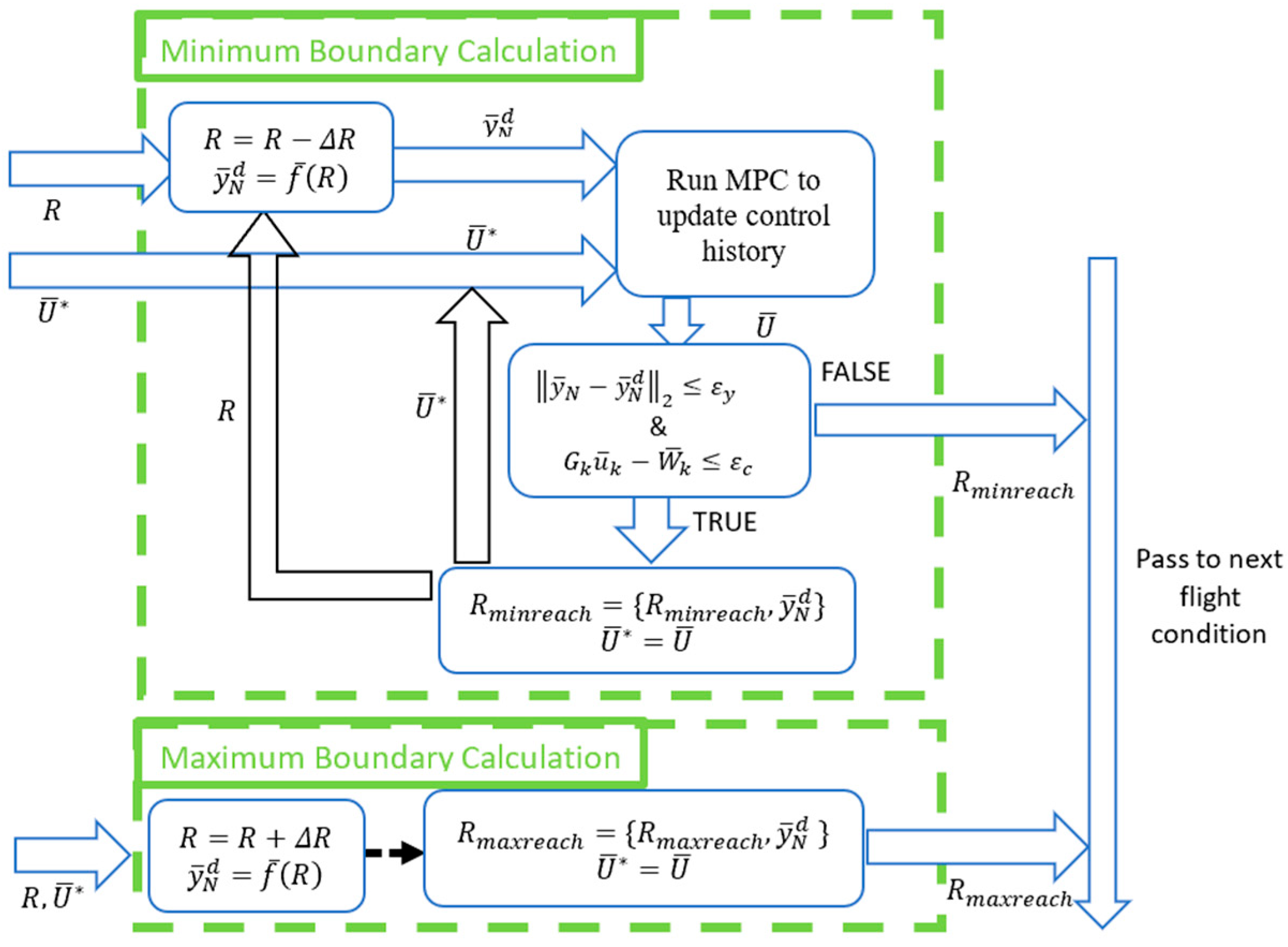
The flowchart for determining reachability boundaries is presented in Figure 5. In the flowchart, ${\overline{y}}_m$ is the output after applying the input history $\overline{U}=\left\{\overline{u}\left(1\right),\overline{u}\left(2\right),\cdots ,\overline{u}\left(N-1\right)\right\}$ of the final iteration. In the flowchart, index is a counter for the current flight condition, and indexMax is the total number of flight conditions to be simulated. The reachable set boundary search logic involves a series of well-defined steps. Before commencing the reachable set computation, it is imperative to establish the flight conditions under which the analysis will be conducted. This entails defining search directions and specifying various flight parameters, such as altitude, Mach number, and other pertinent factors that significantly influence the interceptor’s flight characteristics and performance. The procedure requires defining a terminal desired position, which serves as the target location the interceptor aims to reach at the designated flight duration. Initially, the interceptor is guided toward this target position using the proportional navigation guidance (PNG) approach, which employs guidance laws to minimize the line-of-sight (LOS) rate between the interceptor and the target, thus providing an initial trajectory for the interceptor. The model predictive programming (MPP) approach utilizes the initial input vector obtained through the PNG approach as a starting guess. The algorithm optimizes a cost function to derive a refined solution that minimizes the control effort required throughout the entire flight duration. After computing the solution using the MPP approach, it becomes vital to assess the terminal position error to determine if it falls below a predefined threshold. Additionally, input constraints, such as acceleration limits, are verified for activation. If the terminal position error lies within the specified threshold, and the input constraints are not violated, the computed solution meets the predefined criteria for reachability. In cases where the conditions specified are not satisfied, there is no need to execute calculations for the minimum and maximum reachability boundaries for the current flight condition. In such instances, the analysis proceeds to another flight condition, adjusting the parameters as necessary. However, if the specified conditions are met, indicating that the computed solution fulfills the desired criteria, the calculations for the minimum and maximum reachability boundaries are executed accordingly.

4.3.1. Maximum Range Reachability Boundary Computation

Reachability boundaries for maximum flight range are determined, firstly by propagating an initial guess regarding the terminal position of the interceptor in forward search direction (direction for flight range increase) by a chosen step size. Then, MPP is utilized to check the reachability for the updated desired terminal position. If the terminal position error of the interceptor is lower than the tolerance value $\left({ϵ}_{tol}\right)$, and the resultant input vector does not exceed the acceleration limits, the updated terminal position is taken as a candidate for the reachability boundary for maximum range. For each MPP computation, the recently updated input vector history is utilized. The procedure is repeated until the interceptor cannot reach the updated terminal position.

4.3.2. Minimum Range Reachability Boundary Computation

Likewise, the aforementioned procedure is equally employed to ascertain the reachability boundary concerning the minimum flight range. The backward search direction is considered, denoting a reduction in flight range. The identical principles and procedural steps explicated for the analysis of maximum flight range are duly implemented in this context. By propagating an initial estimate of the terminal position in the backward search direction, the procedure endeavors to evaluate the reachability of the updated desired terminal position for the minimum flight range. The MPP approach is harnessed to optimize the cost function, effectively considering input constraints and system dynamics. Subsequently, the terminal position error is assessed, and if it meets the predetermined tolerance threshold and the resultant input vector adheres to the acceleration limits, the updated position is deemed a potential candidate for the reachability boundary regarding the minimum flight range. Figure 6 presents a flowchart that illustrates the procedure for determining reachability boundaries.

4.4. Convergence Properties

The proposed computational framework consists of a nested loop structure: an outer loop that iteratively refines the flight trajectory via MPP, and an inner loop that solves a constrained optimization sub-problem at each step. The theoretical soundness of the approach is established by considering the convergence properties of each component.

The inner loop executes Hildreth’s quadratic programming procedure to solve the optimal control update. This sub-problem is formulated as a convex quadratic program (QP), for which the convergence of Hildreth’s original method is a classic result. The problem’s structure aligns with the class of symmetric positive semidefinite linear complementarity problems. The work in [16] provides formal proof of strong convergence for iterative methods applied to such problems, guaranteeing convergence of the entire sequence under the sole condition that a solution exists. Their analysis, which generalizes Hildreth’s method, confirms the convergence of this inner loop. While the convergence of Hildreth’s procedure for convex problems is well established, practical limitations exist. Convergence may be slow if the solution space is very narrow, or it may not be possible if the input constraints make the terminal equality constraint unattainable. To manage these practical considerations, the implementation imposes an upper limit on the number of iterations for Hildreth’s procedure in addition to its standard convergence criteria.

The outer loop employs the MPP algorithm, which is a successive linearization technique applied to a nonlinear system. It is well established that for nonlinear applications, such methods ensure local convergence to an optimal solution, but not necessarily global convergence [14]. This convergence is conditional on the initial control history being sufficiently close to the final optimal solution. In this work, this condition is practically addressed by initializing the algorithm with a feasible trajectory generated by a proportional navigation guidance (PNG) simulation. This provides a good quality initial guess that places the starting point of the optimization within the basin of attraction for the solution.

Therefore, the proposed framework is built upon theoretically sound components. The inner loop’s convergence is mathematically guaranteed by established results in quadratic programming, and the outer loop’s local convergence is made practically reliable through a good initialization strategy. The practical convergence and performance of this two-level algorithm have been demonstrated with detailed simulation results in our previous work [13].

5. Results and Discussion

In this section, the results and the effect of input constraints on the solution are shown.

5.1. Reachable Set Results for Example Flight Condition

The reachability boundaries for the example flight conditions listed in

Table 1. Initial conditions.

${\mathit{\beta }}_0$ (°)	${\mathit{h}}_0$ (m)	${{\mathit{V}}_{\mathit{M}}}_0$ (m/s)	${\mathit{t}}_{\mathit{g}\mathit{o}}$ (s)	${\mathit{\alpha }}_{\mathit{s}\mathit{e}\mathit{a}\mathit{r}\mathit{c}\mathit{h}}$ (°)	${\mathit{\beta }}_{\mathit{s}\mathit{e}\mathit{a}\mathit{r}\mathit{c}\mathit{h}}$ (°)
40	0	200	15	$0,20,40,60,80$	$-30,-15,0,15,30$

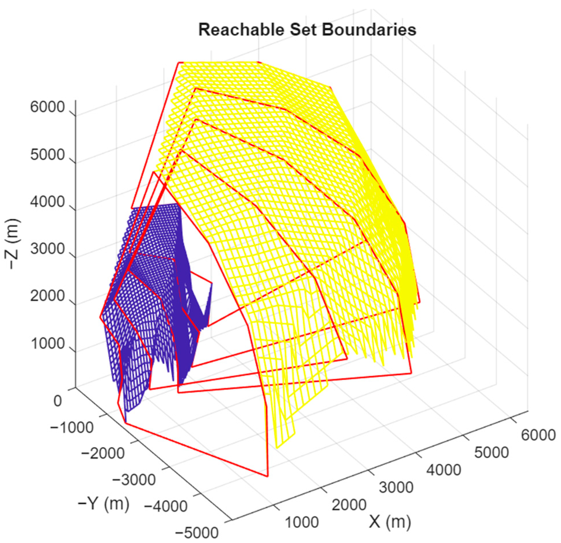
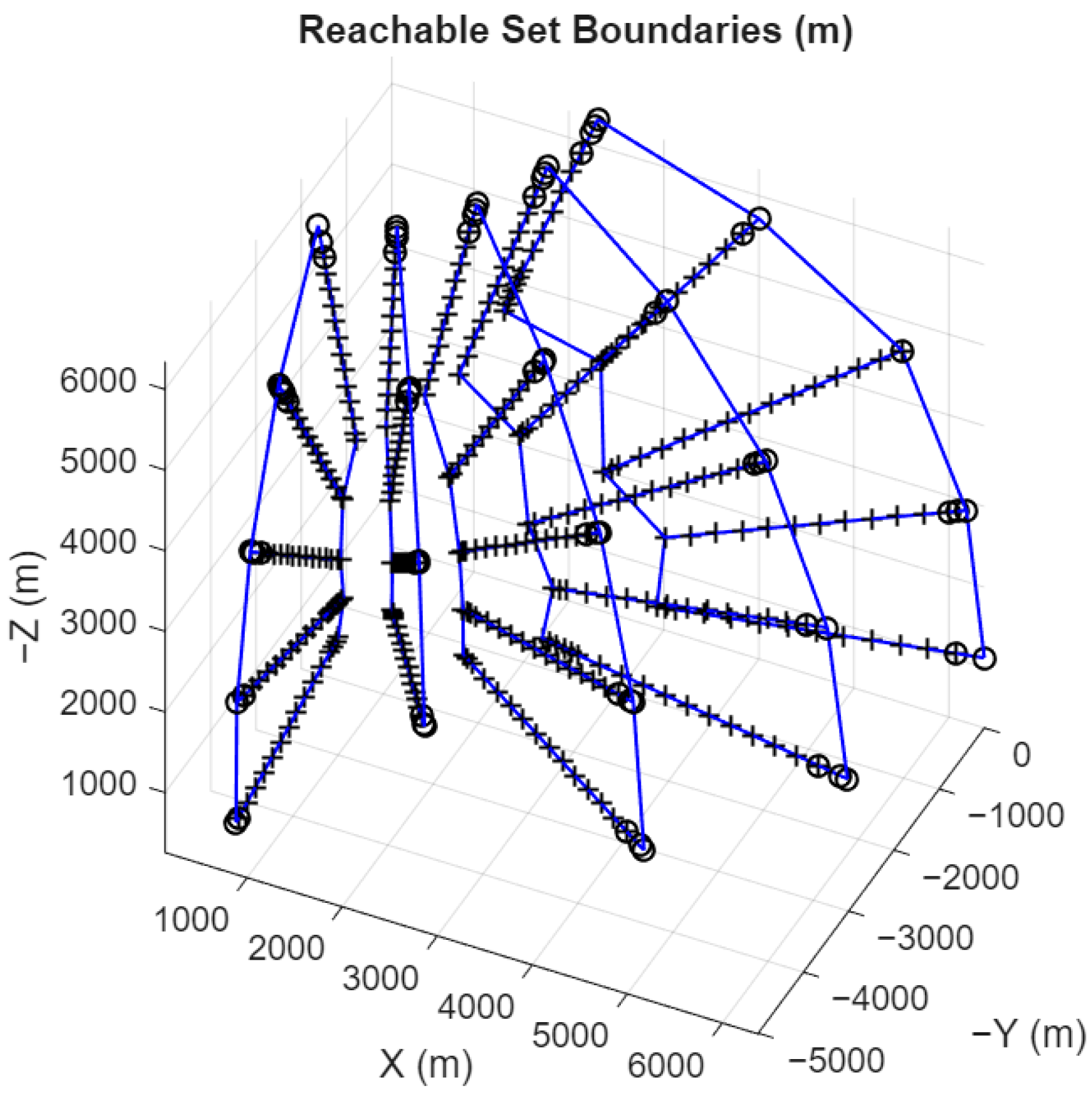
have been computed. Figure 7 illustrates the reachable set boundaries for the selected initial conditions. Yellow and blue surfaces depict the maximum and minimum reachability boundaries for a given set of $({\alpha }_{search},{\beta }_{search})$. The red lines indicate reachability boundaries corresponding to various ${\alpha }_{search}$ values. Figure 8 presents the reachable points, where black markers denote the reachable points, and the blue lines represent the reachability boundaries for different ${\alpha }_{search}$ values.

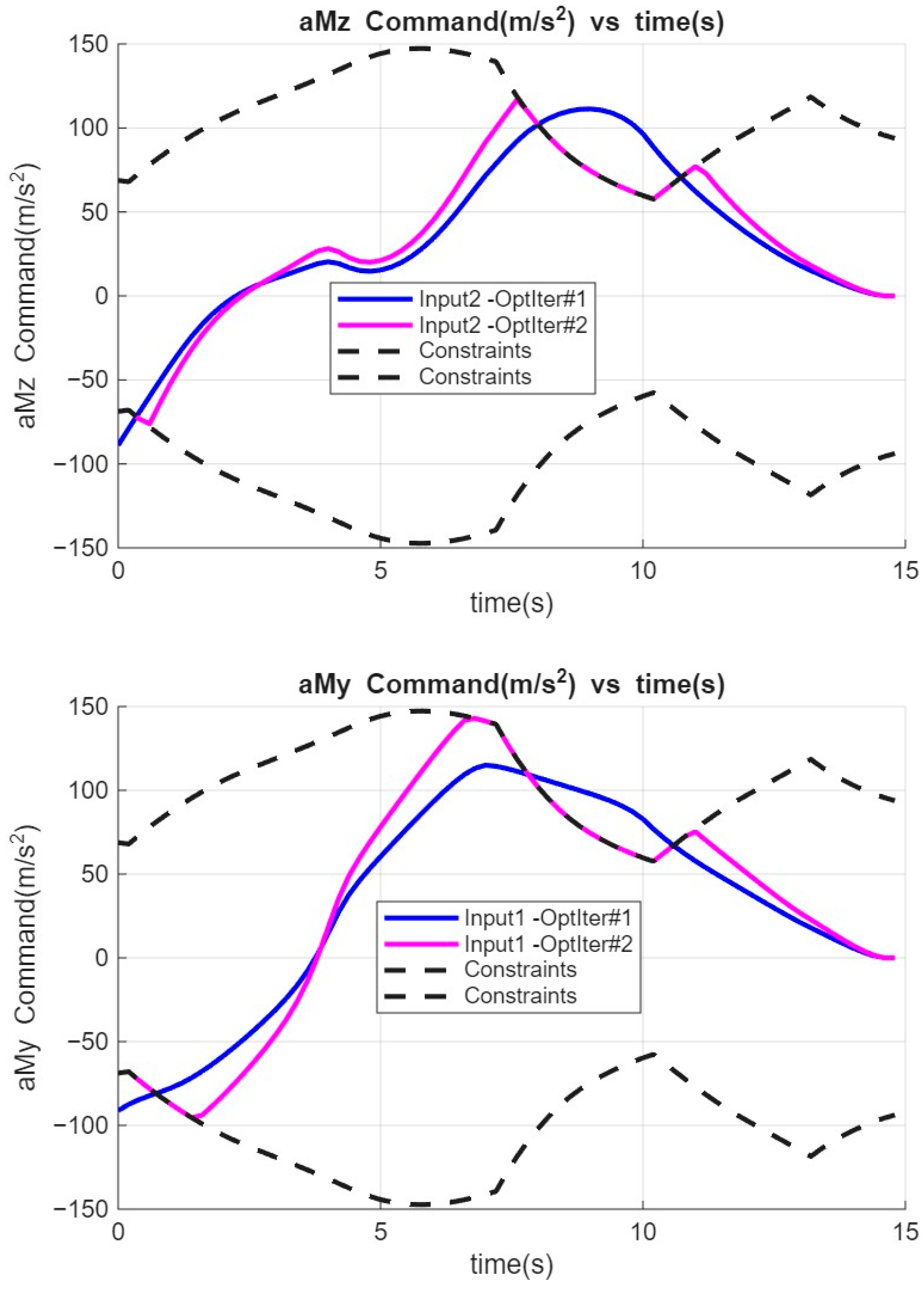
Figure 9 shows lateral acceleration commands for ${\alpha }_{search}=0°$ and ${\beta }_{search}=0°$. Blue and pink lines represent the first and second MPP iteration results, respectively. Black dashed lines represent the upper and lower acceleration limits. Figure 10 shows the trajectories for the first and second MPP iteration and the desired terminal position.

It is important to note that the input-constrained MPP calculation starts if the terminal position error of the unconstrained MPP solution is smaller than the acceptable tolerance value and if the resultant input vector exceeds acceleration limits, as illustrated in Figure 9. Since the input vectors from the unconstrained MPP solution exceed the upper acceleration limits required to reach the desired terminal position, input-constrained MPP calculations are performed to determine the Lagrange multipliers associated with the input constraints. Figure 9 and Figure 10 show how the input-constrained MPP approach adjusts the initial input vector to simultaneously satisfy both the terminal position and the input constraints.

Figure 11 and Figure 12 depict the maximum and minimum reachability boundary for the 15 s flight duration case. Figure 11 presents these boundaries in a 3D view, while Figure 12 provides their 2D projection in the X-Y plane.

5.2. Reachable Set Results for Different Initial Conditions

Figure 13 demonstrates the reachability boundaries obtained for various flight durations, for search angle values specified in Table 1, considering input constraints. It is observed that the interceptor’s capability to travel longer distances increases with the extension of flight duration, provided it possesses sufficient energy.

Figure 14 and Figure 15 demonstrate the reachability boundaries for different initial altitudes and initial velocities. It should be noted that the initial path angle (${\beta }_0$) and flight duration is set as $40°$ and 15 s, respectively, in this analysis. These figures demonstrate the reachability boundaries obtained for different search angle values (${\alpha }_{search}=0°,15°,\cdots ,80°$ and ${\beta }_{search}=-25°,-10°,10°,25°,30°$). It is evident from these figures that the reachability boundaries shift and expand with higher initial altitude and velocity. Furthermore, it is essential to emphasize that both the area and shape of the reachable set are subject to substantial influence by variations in initial altitude and velocity.

5.3. Reachable Set Comparison Between Unconstrained Input Case and Input Constraint Case

In this section, the effect of input constraints on the reachability boundary is demonstrated by a comparison of test cases 1 and 2, as shown in

Table 2. Initial conditions.

Test Case	${\mathit{\beta }}_0$ (°)	${\mathit{h}}_0$ (m)	${{\mathit{V}}_{\mathit{M}}}_0$ (m/s)	${\mathit{t}}_{\mathit{g}\mathit{o}}$ (s)
1	30	0	200	15
2	10	0	200	15

. Reachability boundaries are obtained by utilizing the MPP approach for different search angles.

Figure 16 and Figure 17 illustrate the reachability boundaries for two test cases (Test Case 1 and Test Case 2). The red lines depict the reachability boundaries derived under constrained input conditions, while the blue lines represent the boundaries for an unconstrained input scenario. The analysis reveals that imposing acceleration constraints significantly reduces the extent of the minimum range reachability boundaries. This reduction is evident, with the constrained input cases showing a contraction of up to 3700 m compared to their unconstrained counterparts. Such constraints highlight the influence of limitations on achievable trajectories and emphasize the need for their consideration in realistic reachability analyses.

For Test Case 2, the impact of maximum range reachability boundaries is particularly notable. As ${\alpha }_{search}$ values increase, the difference between constrained and unconstrained cases grows, with a maximum deviation of approximately 1100 m. This observation underscores the sensitivity of maximum range calculations to input constraints and demonstrates the role of acceleration limits in shaping the reachable regions.

5.4. Sensitivity Analysis of Reachability Boundaries

A sensitivity analysis was performed to examine how variations in system parameters influence the reachable set of aerodynamic interceptors. The study utilized a range of simulations, introducing perturbations in drag coefficients and thrust levels, as summarized in

Table 3. Different perturbation cases.

Scenario Description	Perturbed Parameter	Scenario Number	Perturbation Percentage (%)
Nominal	-	1	-
Base Drag Coefficient Variation	$C_{X,0}$	2	−20
		3	−10
		4	+10
		5	+20
Acceleration Related Drag Coefficient Variation	$C_{X,a}$	6	−20
		7	−10
		8	+10
		9	+20
Pulse 1 Thrust Variation	$T_{p1}$	10	−20
		11	−10
		12	+10
		13	+20

. These perturbations provided insights into how changes in these parameters affect the reachability characteristics.

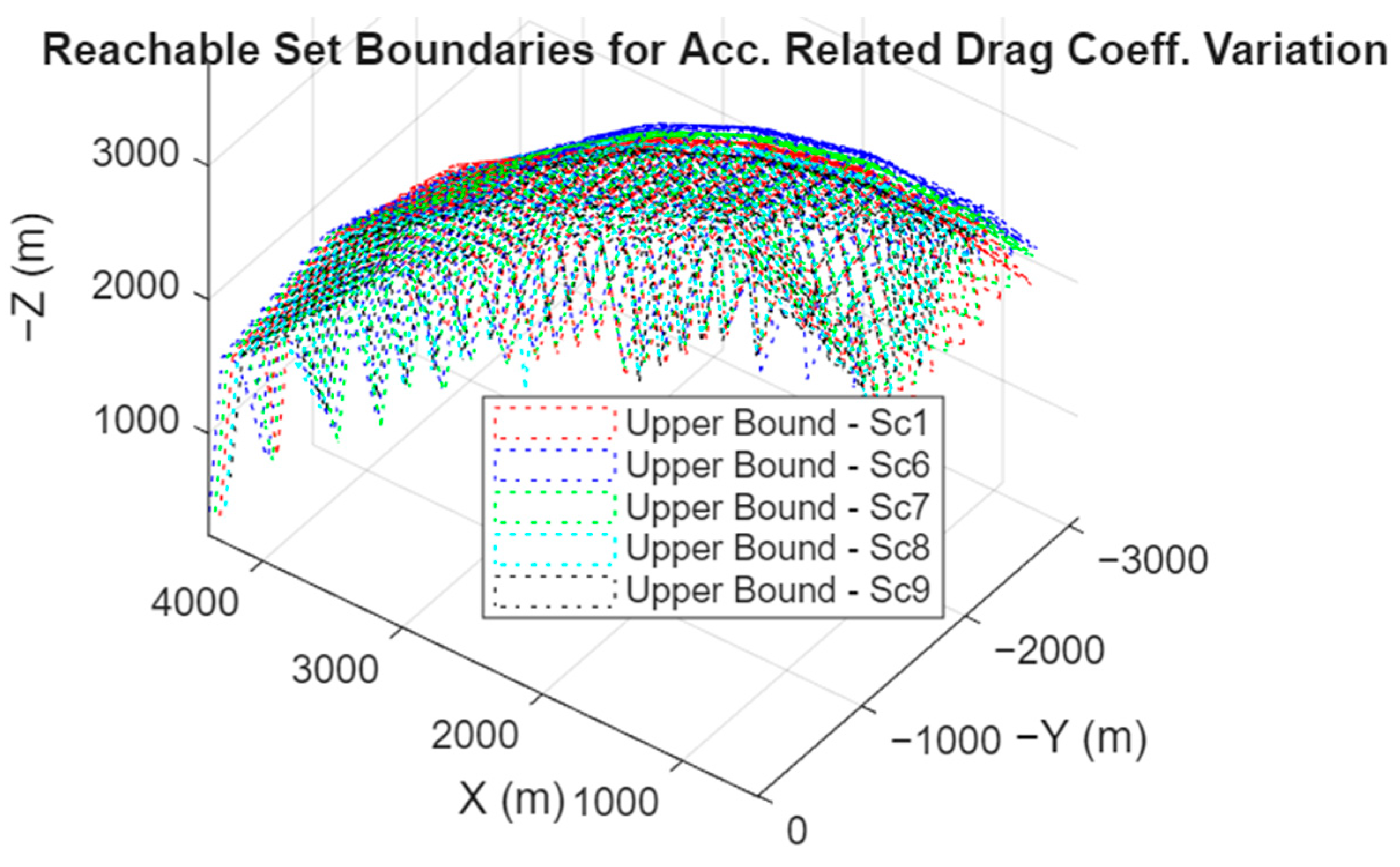
Figure 18 and Figure 19 depict the changes in reachable sets due to variations in base drag and acceleration-related drag values, respectively. For scenarios Sc2, Sc3, Sc6, and Sc7, reductions in drag coefficients caused the reachability boundaries to expand, attributed to decreased aerodynamic resistance. This reduction enables the interceptor to retain higher energy levels, thereby increasing its range. Interestingly, the minimum range boundaries are more significantly affected than the maximum boundaries. This is primarily due to the frequent activation of inequality input constraints for shorter terminal distances, which necessitates higher acceleration commands within the same flight duration. Furthermore, reachability boundaries exhibit uniform scaling across all directions, maintaining their geometric shape while expanding or contracting.

Figure 20 shows how thrust variations impact the reachability boundaries. Higher thrust levels (Sc12 and Sc13) significantly increase the maximum range, as greater thrust provides more energy for longer-distance maneuvers. Consequently, this enhances the interceptor’s effectiveness for long-range missions, offering valuable data for energy optimization and range trade-off analyses.

6. Conclusions

This paper presents a novel computational framework for determining the reachable set boundaries for aerodynamic interceptors, explicitly accounting for nonlinear dynamics and input constraints. This approach builds upon and extends previous studies [13] by refining the concept of reachability, formalizing reachable set generation as a complete algorithmic procedure, and introducing a new sensitivity analysis framework. Additionally, a model predictive programming (MPP)-based method is employed to solve the underlying constrained optimal control problem, ensuring compliance with both equality and inequality constraints related to system dynamics and input limits.

By employing a directional search technique, the algorithm effectively computes the minimum and maximum boundary points of the reachable set without relying on predefined geometries or predefined grid point positions. Moreover, the algorithm takes advantage of the optimized control input history from previous terminal points as starting guesses for subsequent points to accelerate the convergence process. Notably, this approach is able to generate the boundaries of the reachable set more realistically by incorporating inequality and equality constraints into a time-varying system model under dynamic flight conditions.

The main contributions of this work are threefold. First, we introduce a new computational method that combines directional search with an input-constrained model predictive programming (MPP) approach. This framework effectively computes the boundaries of reachable sets, avoiding the “curse of dimensionality” associated with grid-based methods and the “wrapping effect” common in geometric approximations. Second, the MPP formulation, solved using Hildreth’s procedure, allows for the direct inclusion of complex, state-dependent input constraints, such as acceleration limits that change with flight conditions. Third, a sensitivity analysis framework is proposed, providing a systematic way to evaluate how uncertainties in system parameters, such as drag and thrust, impact the reachable set.

The results underscore the critical influence of input constraints. Specifically, comparisons between the reachable sets computed with and without input constraints highlight the impact of acceleration limits on the shape of the reachability boundaries and the volume of the reachable set. Additionally, it is observed that the volume of the reachable set increases with increasing flight duration and is influenced by the initial velocity and altitude.

A sensitivity analysis was performed to assess the impact of variations in system parameters on the reachable set of aerodynamic interceptors. Simulations introduced perturbations in drag coefficients and thrust levels, revealing that reduced drag coefficients expanded the reachability boundaries due to decreased aerodynamic resistance. Similarly, higher thrust levels significantly extended the maximum range by providing greater energy for long-distance maneuvers. These findings highlight the importance of generating and evaluating reachability sets while accounting for such effects.

The proposed optimization method offers a significant advantage by directly embedding input, state, and control constraints into the calculation of reachability boundaries, thus avoiding complex set operations. However, two limitations should be noted. First, the method converges to locally optimal solutions, which are not guaranteed to be globally optimal. Second, the search along any given direction terminates upon finding the first unreachable point, meaning the algorithm effectively maps the boundary but does not identify potentially reachable zones that may exist beyond an unreachable region.

Future research will proceed in several directions. The framework can be extended to handle cooperative engagement scenarios, using the generated databases to optimize task allocation for multiple interceptors. Furthermore, while this study demonstrated the method for an aerodynamic interceptor, the underlying computational framework is general-purpose and can be adapted to analyze the reachable sets of other autonomous systems by substituting the relevant dynamic models and constraints. Further work will also focus on improving computational efficiency to explore the potential for real-time, onboard implementation. A critical next step will be the validation of computed reachable sets against high-fidelity simulations and, eventually, comparisons with flight test data to confirm the accuracy of the system’s representation. Finally, future efforts could investigate methods to identify disjointed reachable regions to overcome the current search termination limitations.