Transient Simulation of Aerodynamic Load Variations on Carrier-Based Aircraft During Recovery in Carrier Airwake

Abstract

Carrier-based aircraft recovery is a critical and challenging phase in maritime operations due to the turbulent airwake generated by aircraft carriers, which significantly increases the workload of flight control systems and pilots. This study investigates the airwake effects of an aircraft carrier under varying wind direction conditions. A high-fidelity mathematical model combining delayed detached-eddy simulation (DDES) with the overset grid method was developed to analyze key flow characteristics, including upwash, downwash, and lateral recirculation. The model ensures precise control of aircraft speed and trajectory during landing while maintaining numerical stability through rigorous mesh optimization. The results indicate that the minimum lift occurs in the downwash region aft of the deck, marking it as the most hazardous zone during landing. Aircraft above the deck are primarily influenced by ground effects, causing a sudden increase in lift that complicates arresting wire engagement. Additionally, the side force on the aircraft undergoes an abrupt reversal during the approach phase. The dual overset mesh technique effectively captures the coupled motion of the hull and aircraft, revealing higher turbulence intensity along the glideslope and a wider range of lift fluctuations compared to stationary hull conditions. These findings provide valuable insights for optimizing carrier-based aircraft recovery procedures, offering more realistic data for simulation training and enhancing pilot preparedness for airwake-induced disturbances.

1. Introduction

Carrier-based aircraft face rigorous environmental conditions and complex control demands during takeoff and landing, surpassing the challenges encountered by land-based aircraft. During fixed-wing aircraft landing, the carrier typically maneuvers into the wind at a specified speed to reduce the relative velocity upon touchdown and increase airspeed for greater lift. During navigation, the complex structure of the aircraft carrier induces chaotic airwake, accompanied by complex turbulent flow phenomena such as recirculation, flow separation, and vortex shedding [1]. As carrier-based aircraft rapidly approaches the deck with a high descent rate, the required low speed and high angle of attack (AOA) for landing lead to a reduction in lift. The aircraft undergoes a sudden and significant loss of wing lift when entering the turbulent airwake near the carrier’s aft deck edge, a critical condition that places it at high risk of stalling [2].

Furthermore, upon entering the carrier’s airwake vortex system, the aircraft’s flight attitude is disrupted by the carrier’s airwake vortices. Upwash and downwash, compounded by ground effects upon reaching above the deck, result in significant fluctuations in lift. This markedly increases the difficulty of control, particularly in adverse conditions such as high winds, rough seas, ship motion, and low visibility, where the airwake vortex system induces strong nonlinear and unsteady aerodynamic disturbances during the aircraft’s landing process. Additionally, the interaction of the ship’s hull and the approaching aircraft generates coupled airflow, further complicating flow behavior [3].

To address the dynamic interface between ship and aircraft, it is essential to comprehend the aerodynamic airwake patterns of individual vessels. To investigate the flow conditions around the hull, experiments targeting specific ship types were conducted, including field measurements and wind tunnel tests [4,5,6]. The experimental results served as calibration data for numerical simulations. However, experimental research faces limitations in altering ship types and natural conditions such as wind direction and speed. Computational fluid dynamics (CFD) exhibits excellent adaptability, facilitating the alteration of ship structures and external conditions [7,8,9]. CFD has been extensively applied in the study of airwake dynamics for large vessels, with its development evolving from Reynolds-averaged Navier–Stokes (RANS) to large eddy simulation (LES), gradually unraveling finer flow structures. To overcome the high mesh requirements of LES, Spalart et al. [10,11] proposed the detached-eddy simulation (DES) method, which employs RANS near the wall and LES away from it, effectively combining the advantages of both. Forrest et al. [12] utilized DES to investigate the airwake of a simplified frigate shape and the Royal Navy Type 23 frigate under various wind and wave conditions. The results demonstrated that DES resolved turbulent structures that adversely affected shipboard helicopter operations. Watson et al. [13,14] employed DDES to simulate the airwake of an aircraft carrier, with computational results consistent with Doppler velocimetry measurements from water tank experiments, showing an increase in turbulent intensity within the domain as the crosswind angle increases. Nisham et al. [15] applied the DES model, demonstrating that the atmospheric boundary layer reduced both the airwake velocity and the ship motion magnitude induced by vertical waves. Yang et al. [16] employed a hybrid DDES and overset grid methodology, demonstrating that ship heave motion significantly enhances turbulence intensity in the airwake region.

The aforementioned studies primarily focus on individual ship analysis, resolving the disturbance effects of the ship hull and upper structures on the surrounding flow field. However, these studies do not adequately reflect the specific impact on aircraft control. Shipman et al. [17] carried out an unsteady dynamic mesh simulation to study the F/A-18 landing process on CVN-class carriers, revealing increased aircraft lift near the deck and above its aft edge due to ground effect. The dynamic mesh approach demonstrated significant grid deformation during the aircraft’s approach. For the dynamic interface of ships and aircraft, there have been more numerical simulation studies focusing on helicopter landings [18,19,20,21]. Bridges et al. [22] utilized flight dynamics simulation and CFD to analyze the workload during the fully coupled dynamic interface of helicopters and ships. This fully coupled method simultaneously runs pre-existing flight dynamics and CFD analysis codes, sharing data between the two sets of codes. The flight dynamics code provides position and load data, while the CFD analysis code offers local velocity data. Kääriä et al. [23] employed the DES model to examine the turbulent flow patterns trailing a frigate. The study aimed to understand how the ship’s exposure to crosswinds induces abrupt pressure fluctuations in the surrounding airflow, leading to increased flight loads. Forrest et al. [24] utilized CFD and flight simulators to analyze how flow separation at the frigate’s hangar edge affects helicopter controllability. Modification of the hangar edge reduces airflow turbulence on the flight deck, consequently decreasing instability loads on helicopters and pilot workload. Shi et al. [25] combined the DES model with helicopter flight dynamics to establish a one-way coupled numerical approach for the ship–helicopter dynamic interface. This approach was employed to investigate the effects of active and passive flow control on the dynamics interface of ship–helicopter, particularly on control margins and the characteristics of unsteady aerodynamic loads. Su et al. [26] conducted coupled simulation research on rotor loads during the vertical landing of shipborne helicopters using the RANS k-ω turbulence model. They employed an overset grid method to simulate the complex and highly unsteady aerodynamic interactions between the rotors, flight deck, and hangar during vertical landing. Dooley et al. [27,28] utilized the DES model to investigate the impact of atmospheric turbulence, ship motion, and sea wave on the deck flow field. Analysis of the rotor-craft lift response above the deck indicated that ship motion had the most significant influence. Power spectral analysis revealed that helicopter lift was more sensitive to low-frequency fluctuations induced by ship motion and waves. Thedin et al. [29,30] utilized LES to assess the impact of the atmospheric boundary layer on the dynamic interface simulation between the frigate’s airwake and aircraft. Frequency domain analysis of the airwake revealed that the atmospheric boundary layer exerted influence within the 0.1 to 2 Hz frequency band, thereby affecting airflow dynamics and subsequent flight loads.

Most studies obtain flight position data directly from flight simulation software. Research on ship airwake demonstrates that flow separation caused by the ship’s deck edge and superstructure amplifies airflow disturbances significantly influences the aerodynamic forces on aircraft during approach and landing. While extensive research focuses on the dynamic interface between ships and helicopters, studies on fixed-wing aircraft landings remain limited. Fixed-wing aircraft and helicopters differ markedly in approach paths, speeds, and touchdown methods, each presenting distinct challenges. Building upon the isolated carrier airwake research [16], this study introduces coupled carrier–aircraft geometry and multi-zone meshing in the computational domain to quantify airwake-induced aerodynamic load disturbances on the aircraft. The present work utilizes a coupled DDES and overset grid method to simulate the aircraft landing process. The carrier’s airwake is analyzed to assess its impact on aerodynamic force variations during the landing process. Furthermore, the effects of ship heave and pitch motion on airflow disturbances and aircraft control loads are investigated using dual-object overset grids.

This paper is organized into five sections. Section 2 provides a detailed description of the mathematical model equations and the method of DDES coupled with dual-object overset grids. Section 3 elaborates on the geometric model, grid generation, and boundary conditions. Section 4 presents results and discussions. In this section, the flow characteristics of the carrier airwake under different wind direction are first compared. This is followed by an analysis of the influence of the airwake on the forces acting on the aircraft. Finally, the enhanced disturbance of the aircraft lift induced by the heave and pitch motion of the carrier is analyzed. Section 5 summarizes the important findings of this paper.

2. Numerical Method

There are three main issues that need to be addressed by CFD methods during aircraft landings: airwake generated during ship navigation, the method of meshing the dual-object motion of the ship and aircraft, and the burble effect on the forces of the aircraft. To simulate the airwake generated by a moving carrier, the relative wind representing ship navigation was modeled using DDES. A combination of DDES and overset grid is used to simulate the carrier and aircraft motions. In order to take into account the effect of airwake turbulence enhanced by the heave and pitch motion of aircraft carriers on the flight control, double overset grids are used. Each grid region represents the motion of the carrier in the vertical direction and the aircraft approach motion, respectively. The variation in aircraft lift from approach to touchdown is analyzed by comparing the simulation results.

2.1. DDES Numerical Method

While LES can resolve fine-scale flow features, its stringent grid resolution requirements lead to prohibitively large computational costs for full-scale simulations. DDES combines LES with RANS modeling, avoiding the limitations of LES. In this model, the near-wall region uses the SST k-ω turbulence model, while the free shear flow away from the wall is handled by LES. This method efficiently transitions from RANS to LES and is suitable for numerical calculations of full-scale models on the order of hundreds of meters. However, unambiguous grids near the wall pose a challenge for complex geometries of large hulls. DDES improves upon traditional approaches through a generalized formulation that simultaneously accounts for grid scale and wall distance effects [11,31].

Equations (1) and (2) are the transport equations for turbulent kinetic energy and dissipation rate, respectively:

$${\displaystyle \frac{\partial \left(\rho k\right)}{\partial t}}+{\displaystyle \frac{\partial \left(\rho u_{j}k\right)}{\partial u_j}}=P_k-\rho {\displaystyle \frac{k^{3/2}}{l_{DDES}}}+{\displaystyle \frac{\partial }{\partial x_j}}\left[\left(\mu +{\displaystyle \frac{{\mu }_t}{{\sigma }_k}}\right){\displaystyle \frac{\partial k}{\partial x_j}}\right]$$

(1)

$${\displaystyle \frac{\partial \left(\rho \omega \right)}{\partial t}}+{\displaystyle \frac{\partial \left(\rho u_j\omega \right)}{\partial u_j}}={\displaystyle \frac{\partial }{\partial x_j}}\left[\left(\mu +{\displaystyle \frac{{\mu }_t}{{\sigma }_{\omega }}}\right){\displaystyle \frac{\partial \omega }{\partial x_j}}\right]+2\left(1-F_1\right){\displaystyle \frac{{\sigma }_{\omega 2}\rho }{\omega }}{\displaystyle \frac{\partial k}{\partial x_j}}{\displaystyle \frac{\partial \omega }{\partial x_j}}+\alpha {\displaystyle \frac{\rho }{{\mu }_t}}{P}_k-\beta \rho {\omega }^2$$

(2)

$${\mu }_t=\rho {\displaystyle \frac{a_{1}k}{\max \left(a_1\omega ,F_{2}S\right)}}$$

(3)

where k is the turbulent kinetic energy. ω is the specific dissipation rate. ρ is the density. u_j is the velocity component. x_j is the spatial coordinate component. μ is the dynamic viscosity. μ_t is the turbulent viscosity. σ_k and σ_ω are model constants used to control unsteadiness. P_k is the production of turbulent kinetic energy. F₁ and F₂ are the blended function.

$$F_1=\tanh \left({\arg }_1^4\right)$$

(4)

$${\arg }_1=\min \left(\max \left({\displaystyle \frac{\sqrt{k}}{C_{\mu }\omega y}},{\displaystyle \frac{500\nu }{y^2\omega }}\right),\begin{array}{c}\end{array}{\displaystyle \frac{4\rho {\sigma }_{\omega 2}k}{C{D}_{k\omega }{y}^2}}\right)$$

(5)

$$C{D}_{k\omega }=\max \left(2\rho {\sigma }_{\omega 2}{\displaystyle \frac{\nabla k\cdot \nabla \omega }{\omega }},\begin{array}{c}\end{array}{10}^{-10}\right)$$

(6)

$$F_2=\tanh \left({\arg }_2^2\right)$$

(7)

$${\arg }_2=\max \left({\displaystyle \frac{2\sqrt{k}}{C_{\mu }\omega y}},\begin{array}{c}\end{array}{\displaystyle \frac{500\nu }{\omega y^2}}\right)$$

(8)

$$P_k=\min \left({\mu }_t{S}^2,\begin{array}{c}\end{array}10C_{\mu }\rho k\omega \right)$$

(9)

where y represents the distance to the nearest wall, ν is the kinematic viscosity.

The l_DDES length scale in Equation (1) reads as follows:

$$l_{DDES}=l_{RANS}-f_d\max \left(0,\begin{array}{c}\end{array}{l}_{RANS}-l_{LES}\right)$$

(10)

$$l_{RANS}={\displaystyle \frac{\sqrt{k}}{C_{\mu }\omega }}$$

(11)

$$l_{LES}=C_{DDES}\Delta$$

(12)

$$C_{DES}=C_{DES,k-\omega }{F}_1+C_{DES,k-\epsilon }\left(1-F_1\right)$$

(13)

where Δ is the maximum edge length of the cell. The hybrid function f_d in Equation (10) is expressed by the following relationship:

$$f_d=1-\tanh [{(C_{d1}{r}_d)}^{C_{d2}}]$$

(14)

$$r_d={\displaystyle \frac{{\nu }_t+\nu }{{\kappa }^2{y}^2\sqrt{0.5(S^2+{\Omega }^2)}}}$$

(15)

where S is the magnitude of the strain rate tensor and Ω is the vorticity tensor. The coefficients are as follows:

$$C_{d1}=20,\begin{array}{c}\end{array}{C}_{d2}=3,\begin{array}{c}\end{array}\kappa =0.41,\begin{array}{c}\end{array}{C}_{DES,k-\omega }=0.78,\begin{array}{c}\end{array}{C}_{DES,k-\epsilon }=0.61$$

(16)

The coefficients α, β, σ_k, and σ_ω in the above equation are computed through a linear combination. Take α as an example

$$\alpha ={\alpha }_1{F}_1+{\alpha }_2\left(1-F_1\right)$$

(17)

The coefficients are as follows:

$${\alpha }_1=5/9,\begin{array}{c}\end{array}{\alpha }_2=0.44,\begin{array}{c}\end{array}{\beta }_1=0.075,\begin{array}{c}\end{array}{\beta }_2=0.0828,$$

$${\sigma }_{k1}=0.85,\begin{array}{c}\end{array}{\sigma }_{k2}=1,\begin{array}{c}\end{array}{\sigma }_{\omega 1 }=2,\begin{array}{c}\end{array}{\sigma }_{\omega 2}=1/0.856,\begin{array}{c}\end{array}{C}_{\mu }=0.09,\begin{array}{c}\end{array}{a}_1=0.31$$

(18)

The DDES model achieves a smooth transition from RANS to LES. In this study the DDES model is utilized to compute the effect of the ship’s airwake on the aerodynamic loads during aircraft landing operations.

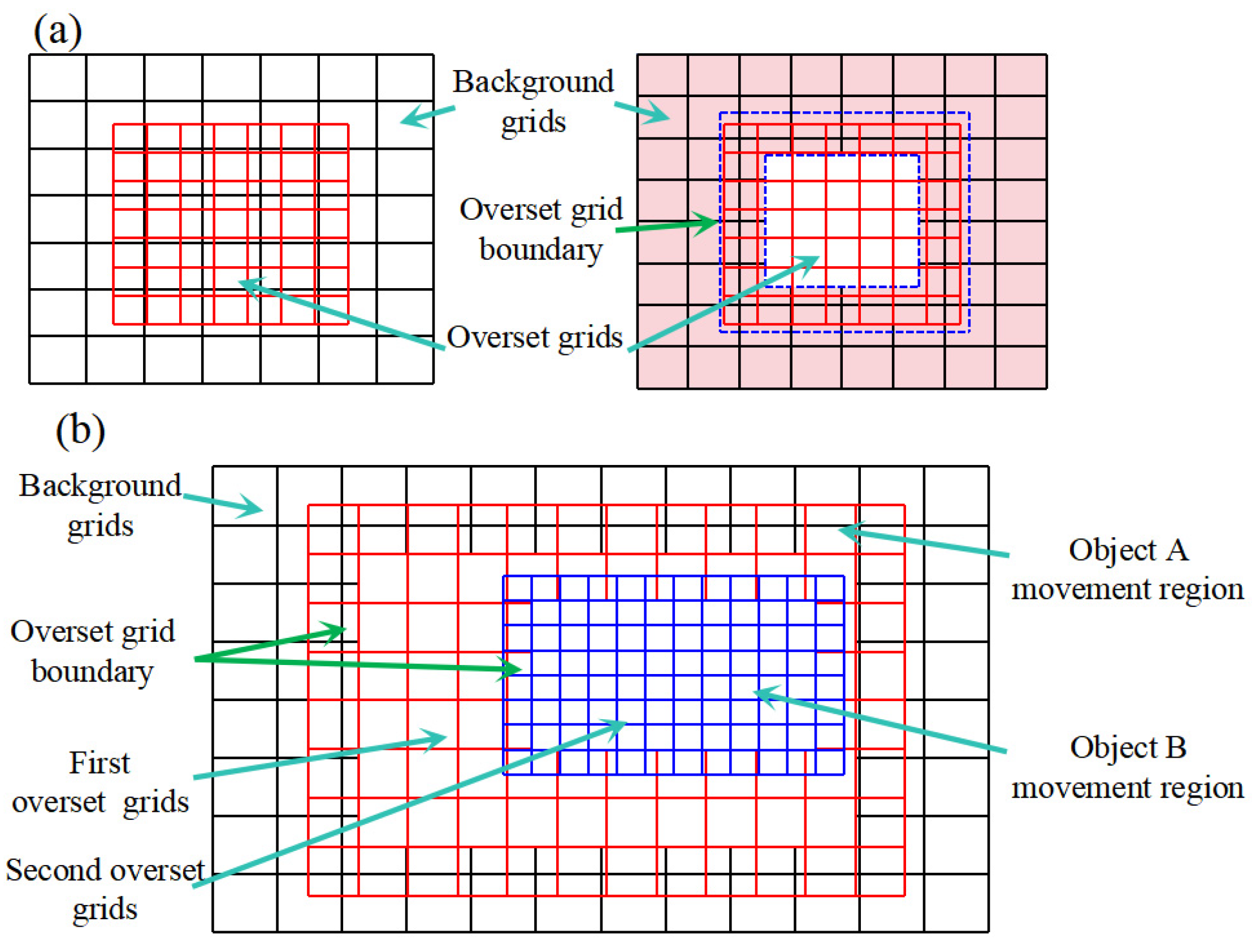
2.2. Overset Grid Method

The overset mesh is more suitable for describing the spatial motion of rigid bodies. During the simulation of object motion, the entire computational domain is divided into a background grid and an overset grid. Separate grids are discretized for the respective solution domains. The numerical transfer between the two sets of grids is performed by interpolation. This approach simplifies the process of reconstructing the topology of the mesh during motion and enhances the generalizability.

The main step in overset meshes is that the computational domain is first decomposed into subregions. The overall computational domain is a background grid, and moving object is divided by a separate sub-area grid. The sub-area grid is the overset grid. Thus a part of the background mesh area covered by the overset mesh becomes outside the computational domain. It is then necessary to dig out the mesh outside the computational domain. Finally, an accurate and efficient interpolation calculation is performed at the junction of the overset grid and the background grid. The final result is an integrated flow field in the computational domain.

Figure 1 is a schematic diagram of the overset grid. It describes the regions of the overset grid for single-body and dual-body motions. During single-body motion, there is only one set of background mesh and overset mesh regions. For the motion of multiple bodies, a dual overset grid is utilized, comprising three regions of computational grids across the entire computational domain. To prevent interpolation confusion resulting from object B crossing the boundary of object A’s overset grid, the overset grid of object A encloses the area of object B’s overset grid, ensuring numerical stability throughout the computational process. This facilitates the simultaneous movement of both the ship and the aircraft. The independent coordinates are synchronized with the ship and aircraft travel.

3. Numerical Details

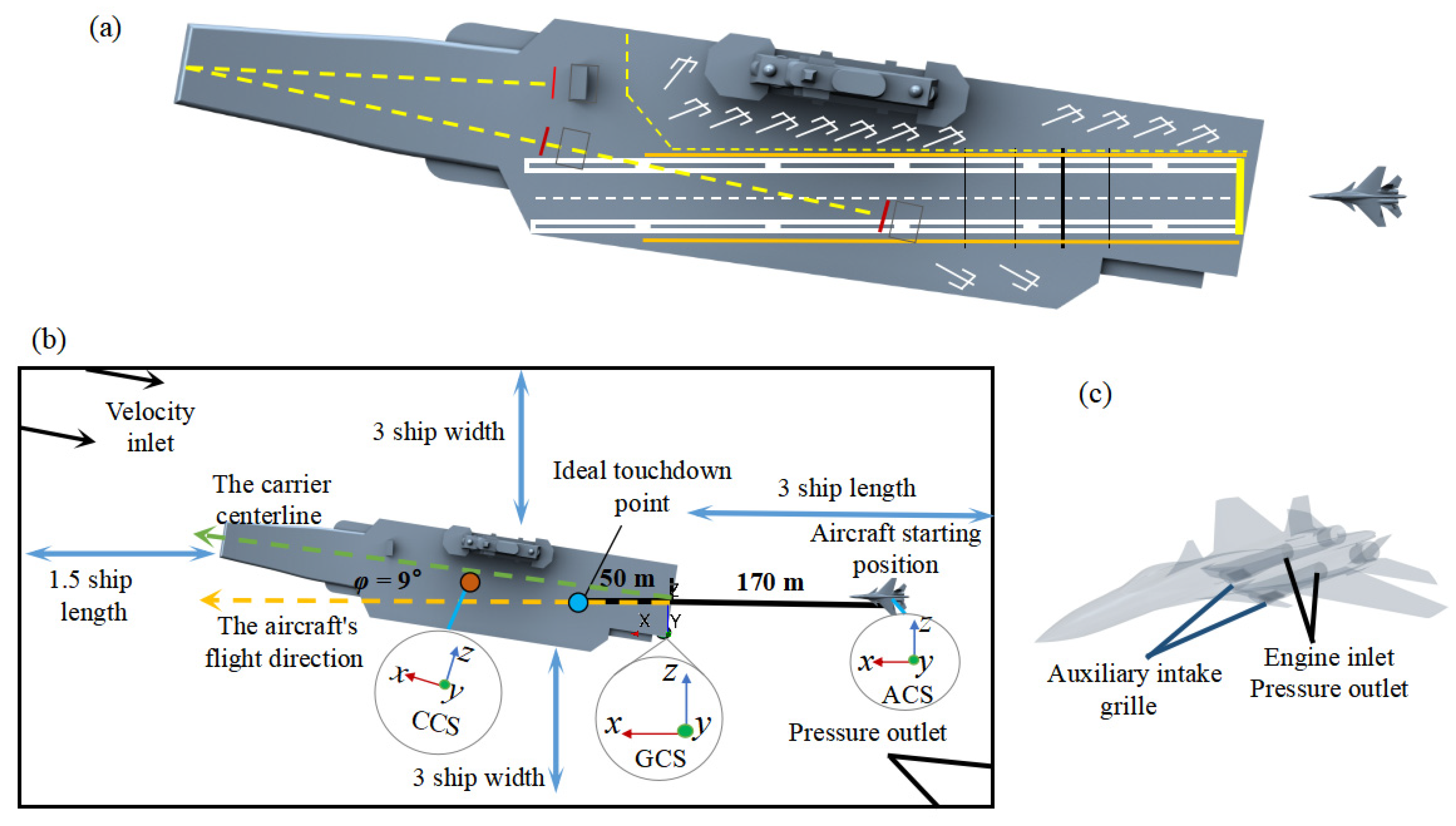
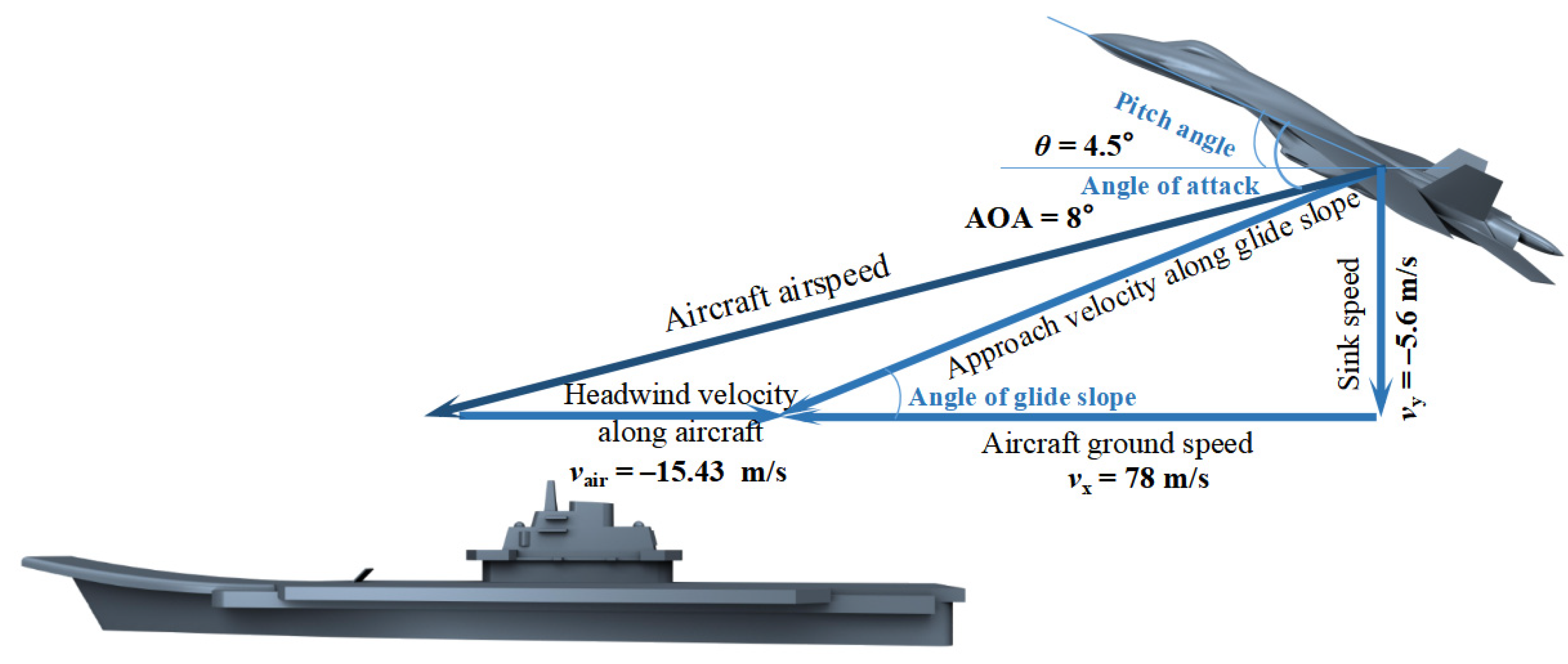
3.1. Geometry Models and Boundary Conditions

This study focuses on the recovery process of carrier-based aircraft on ski-jump-equipped aircraft carriers. The aircraft carrier travels at a typical speed of 30 knots (15.43 m/s). Aircraft circle around to the rear of the carrier and approach to land on the deck, while the carrier travels into the wind. This landing procedure maximizes the aircraft’s airspeed to ensure sufficient lift and minimizes the relative velocity between the aircraft and the carrier. It also results in the lowest relative velocity between them, alleviating the pilot workload, decreasing the difficulty of using the landing guidance system operation, and mitigating the impact on the aircraft structure and carrier arresting equipment during landing.

The geometric models were established using SolidWorks2021 software, as shown in Figure 2a, with key parameters detailed in

Table 1. The key geometric parameters of the aircraft carrier and the aircraft.

Structure	Value
Aircraft carrier length	304 m
Horizontal deck height	16 m
Deck width	68 m
Island height	27 m
Displacement	6 × 104 t
Aircraft length	22 m
Wingspan	14 m
Aircraft mass	22 t

. The carrier deck features an island on the right side, and the forward section includes jet blast deflectors for aircraft taking off. The go-around runway for aircraft is angled 9° from the carrier centerline. The aircraft aligns directly with the go-around runway during landing. During landing, aircraft engages the arresting cables for braking, ideally catching the second or third cable. The region between the first and second bold lines represents the ideal touchdown area, facilitating engagement with the second arresting cable.

The study focuses on analyzing the influence of the wake flow behind the island and the downwash airflow at the stern on aircraft aerodynamics. The deck surface accounts for ground effect on aircraft lift, while other airflow-disturbing elements such as parked aircraft and blast deflectors are simplified [13]. Since the simulation assumes the aircraft comes to a complete stop upon deck landing, arresting cables and braking systems are omitted to avoid unnecessary complexity. No-slip boundary conditions are applied to the walls, which is a standard treatment for such simulations [21].

The carrier-based aircraft is a twin-engine heavy fighter with a duck-wing configuration. The under-fuselage engine configuration demands rapid thrust augmentation during critical flight phases like landing and go-arounds. The auxiliary intake grilles at the base of the inlet ducts open during go-around maneuvers. This supplemental airflow significantly increases engine thrust, enabling the aircraft to reach the required go-around speed if it fails to engage the arresting wires. In the figure, GCS is global coordinate system. CCS is aircraft carrier coordinate system. ACS is aircraft coordinate system.

Figure 2b depicts the boundary conditions and dimensions of the computational domain. A three-dimensional computational domain spanning 300 m height is constructed to resolve the carrier airwake dynamics. When the wind direction is 0°, the inlet face serves as a uniform velocity inlet. The upper, left, and right faces are symmetry planes. The outlet represents a pressure outlet [3,32]. In the simulations, the velocity of wind and ship are coplanar with the ocean surface [7]. When changing the wind direction, taking the starboard side as an example at 45°, the front and right boundaries are set as velocity inlets. Due to the carrier’s 9° deviation, the angle between the air velocity direction and the x-axis is 54° for both boundaries. The left and stern boundaries serve as pressure outlets. Changing the angle of wind is accomplished by combining boundary conditions with the initial flow field velocity direction. The wind direction angles are set as follows: 0° is relative to the aircraft, while left and right deviations of 15° and 45° are relative to the ship. The origin of the global coordinate system is defined at the left aft corner of the ship’s stern deck, with the aircraft’s flight direction aligned along the positive x-axis and the vertical upward direction aligned along the positive y-axis. Independent Cartesian coordinate systems are established at the respective centers of gravity of the ship and aircraft to describe their motion. In the aircraft carrier’s coordinate system, the x-axis is aligned with the ship’s centerline.

The high-speed airflow entering the engine intakes significantly affects lift, necessitating the inclusion of engine inlets in the model. The engine inlets are treated as pressure outlets with a numerical value of −25,000 Pa, as shown in Figure 2c. The jet exhaust contributes to the aircraft’s thrust. At high speeds, however, the exhaust primarily influences the flow field behind the aircraft without directly affecting the aircraft body. Thus, the high-temperature gases emitted from the jet exhaust are neglected in this study.

Figure 3 illustrates the velocity relationship between the ship’s velocity, aircraft speed, and descent rate. The relative wind boundary condition computationally emulates the carrier’s navigation velocity. The entire computational domain is initialized with a speed of 15.43 m/s, which is also applied at the inlet boundary. The aircraft utilizes a hard landing technique, maintaining a constant descent rate to touch down directly on the deck. The aircraft’s velocity components are as follows: v_x = 78 m/s, v_y = −5.6 m/s, pitch angle θ = 4.5°, and AOA = 8.1°.

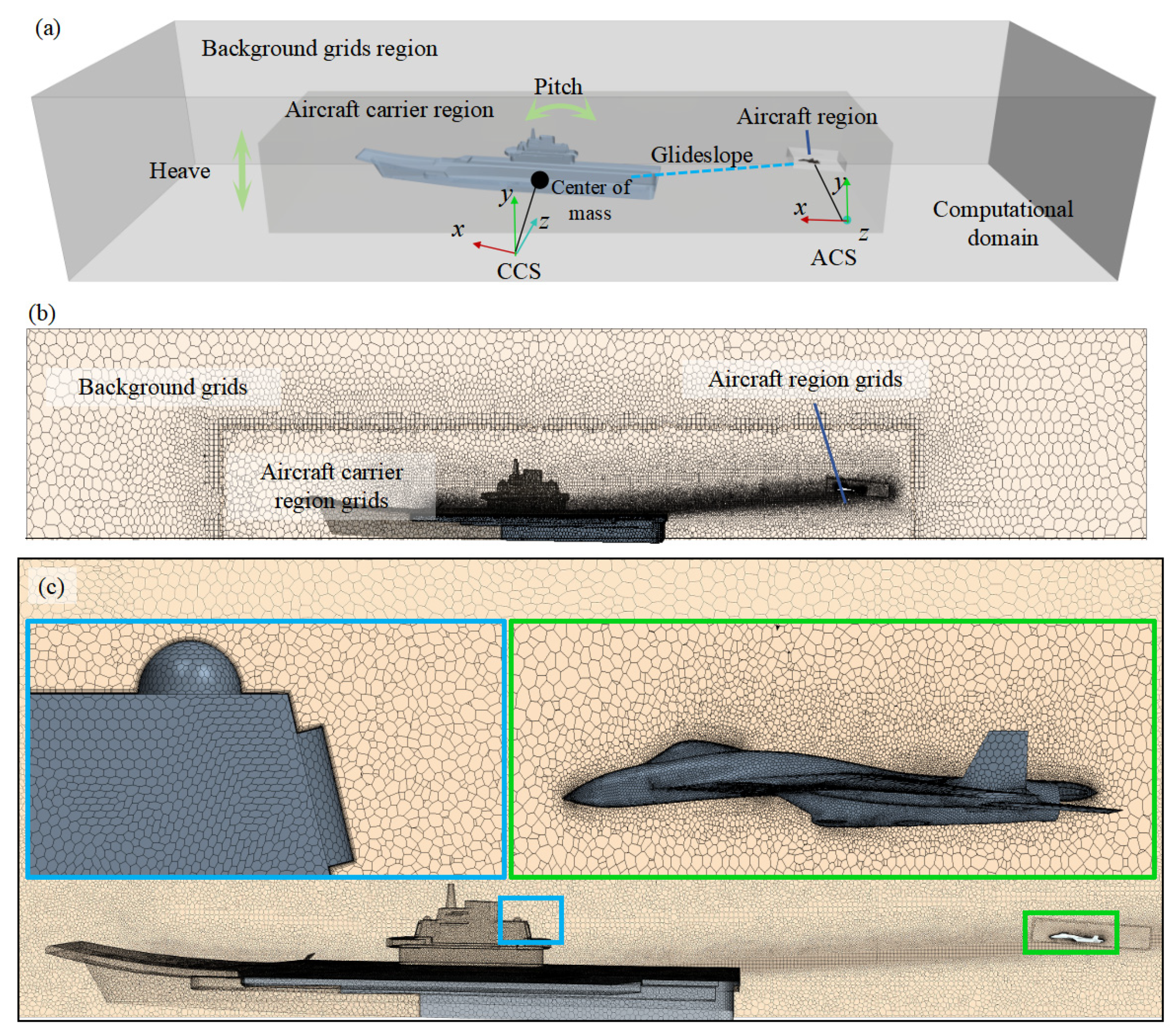
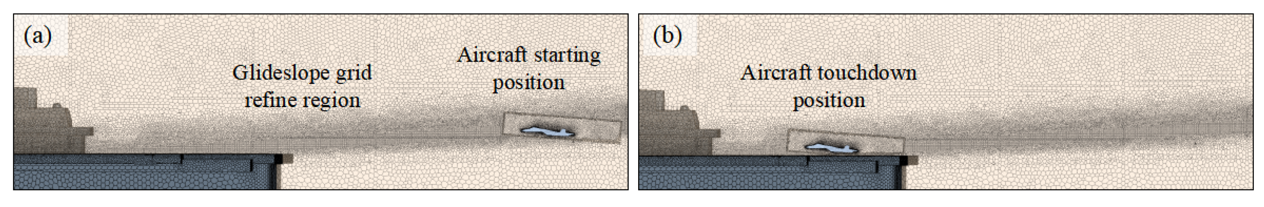
3.2. Grid Generation

Although detailed geometries of aircraft carriers and aircraft have been simplified, complex models are difficult when generating structured meshes. Polyhedral meshes are utilized to discretize the geometry model. The polyhedral grid consists of a combination of dodecahedra and tetrahedra, demonstrating efficiency and adaptability to complex models. To ensure numerical stability, several requirements are fulfilled during the discretization of overset grid. The overset grid region fully encompasses the moving object, with at least 4 to 5 layers of grid between the overset grid boundary and the geometry model. The grid size difference at the interface between the overset grid and the background grid remains within a factor of 2.5.

Figure 4 shows the grids for the aircraft carrier and the aircraft. Three independent grid regions are created within the computational domain, including the background grid region, the aircraft carrier region, and the aircraft region. Grid refinement is applied to critical areas such as the aircraft carrier’s island, deflector plates, aircraft intakes, and grilles. The boundary layer meshes are generated near the wall surface of the object, with a total of 12 layers. The thickness of the first layer of the mesh is 0.005 m, with a growth rate of 1.2. After multiple mesh refinements, the wall y+ values are maintained at approximately 30, which is consistent with the value reported in research [13].

To prevent computational instability caused by the aircraft crossing the boundary of the ship’s overset grid during approach, the rear boundary of the overset grid is positioned 260 m from the ship’s stern. The grid region of the carrier fully encloses the region of the aircraft. To ensure a smooth transition of the grid to the background grid and to accurately capture the airwake generated by the aircraft, the distance from the rear boundary to the tail of the aircraft is set to twice the length of the fuselage. The height from the top to the aircraft body exceeds three times the height of the fuselage. Local grid refinement is applied to the aircraft region to resolve small-scale features like grilles, which are orders of magnitude smaller than the carrier dimensions. The distance between the underside of the aircraft and the deck is only 1.8 m during aircraft touching the deck. Hence, the grid requires rapid refinement from the grilles to the bottom boundary to maintain resolution continuity. In the carrier grid region, it is necessary to refine the grid along the glideslope to ensure smooth grid connection between the two.

3.3. Grid Independence Validation

To ensure the accuracy and reliability of the numerical simulations, a grid independence study is conducted using the average velocity along the glideslope as the benchmark, as shown in Figure 5. The results indicate that the velocity profiles between the 22 million and 25 million grids converge, demonstrating that the resolution of 22 million grids provides sufficient accuracy while maintaining computational efficiency. Therefore, the 22 million grid is selected for all subsequent simulations. This grid independence validation ensures that the numerical results are not influenced by grid resolution and can reliably capture the flow characteristics during the aircraft landing process.

At the beginning of the simulation, the aircraft’s center of gravity is positioned 170 m from the aft edge of the deck and remains stationary. Once the airflow fully traverses the computational domain and forms the airwake region, the aircraft initiates the landing procedure. Load variations are recorded after the aircraft travels a distance of 20 m. The time step during the stationary phase of the aircraft is set to 0.01 s.

When the aircraft begins to move, the numerical stability deteriorates as/because the aircraft speed significantly exceeds the airflow velocity. Residual analysis of the continuity equation during carrier landing is shown in

Table 2. Comparison of numerical residuals for different time steps.

Time Step	Residual
	Continuity	x-Momentum
0.003 s	Divergency	Divergency
0.002 s	10−1	3 × 10−2
0.001 s	1.2 × 10−3	2 × 10−4
0.0005 s	10−3	10−4

. The results reveal that the computation achieves a residual of 1.2 × 10⁻³ at a time step of 0.001 s, meeting the accuracy requirements. The time step during the aircraft motion phase is set to 0.001 s. The finer time step during the dynamic phase ensures adequate resolution of transient aerodynamic interactions arising from the aircraft’s high relative velocity compared to the ambient airflow.

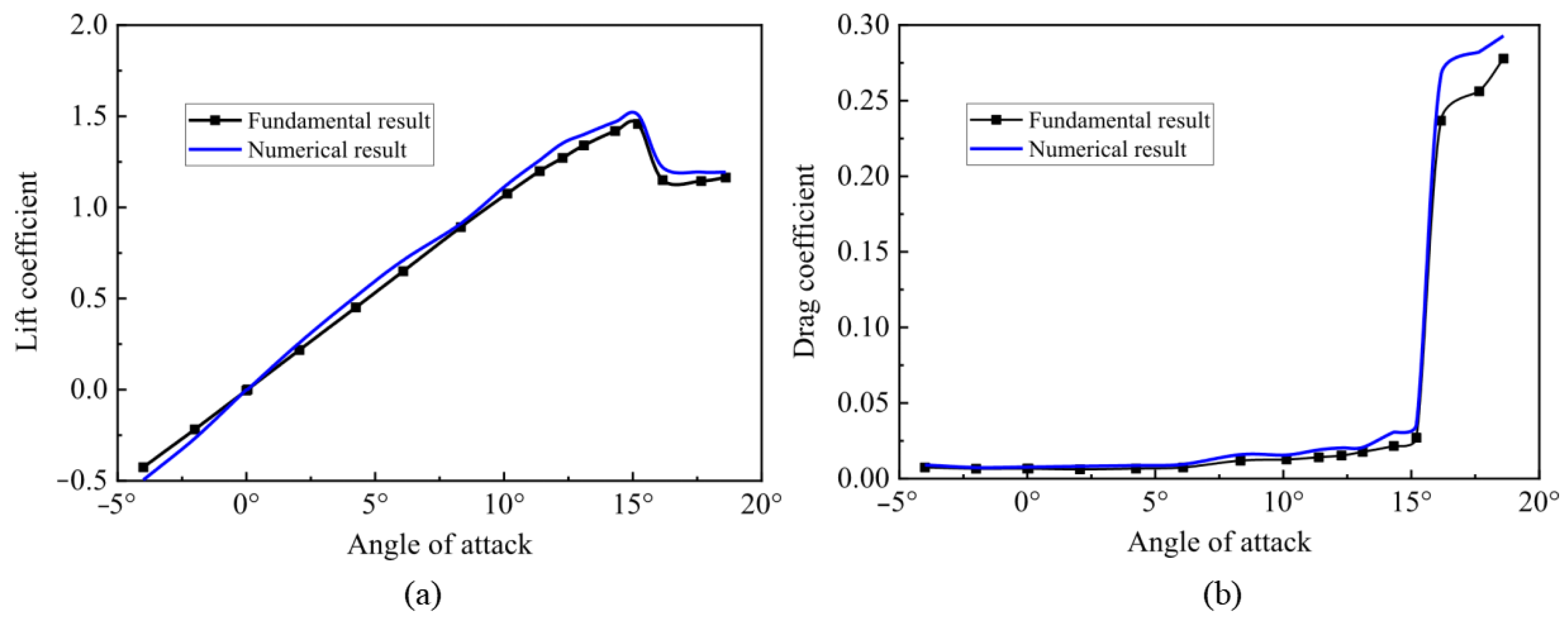
3.4. Validation of Numerical Results

Due to the disturbance from the airwake of the hull during the aircraft landing process, lift force varies continuously. Initially, the computational domain is simplified to simulate the flight process of a single carrier-based aircraft without the presence of an aircraft carrier. To validate this process, publicly available data for the NACA0012 airfoil profile is used for comparison [33]. The literature provides dimensions for the wing profiles as well as lift coefficient data for different Reynolds numbers and various angles of attack conditions. A rectangular 3D airfoil profile as the geometric model for validation is utilized. The computational domain for the NACA0012 airfoil profile is illustrated in Figure 6. In the wing profile validation calculations, polyhedral grids were employed. The boundary layer’s first layer thickness is set to 1 mm, with a growth rate of 1.2. The total number of grid cells is 10 million. The airfoil grids are depicted in Figure 7. In order to verify the accuracy of DDES coupled with overset mesh, the overset grid was employed in the verification calculation. The diagrams show the position of the wing at an AOA of 0° and 10°, respectively.

Figure 8 illustrates the lift variation with AOA at a Reynolds number of 3.29 × 10⁶. The values in the literature serve as the fundamental result in the figure. Comparing with the literature, the numerical result generally agrees with the fundamental result. This suggests that the numerical methods and grid partitioning techniques can be applied to calculate aircraft flight processes aboard carriers.

4. Results and Discussion

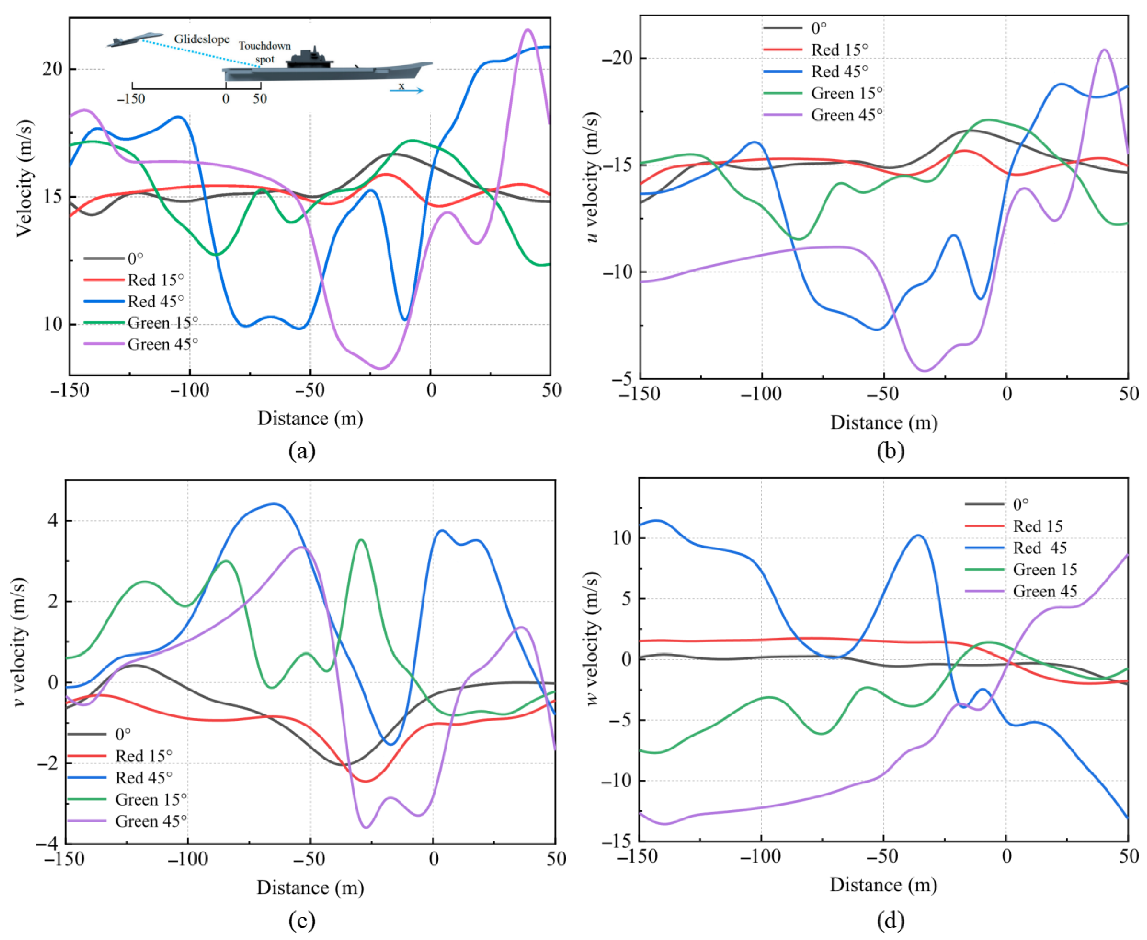
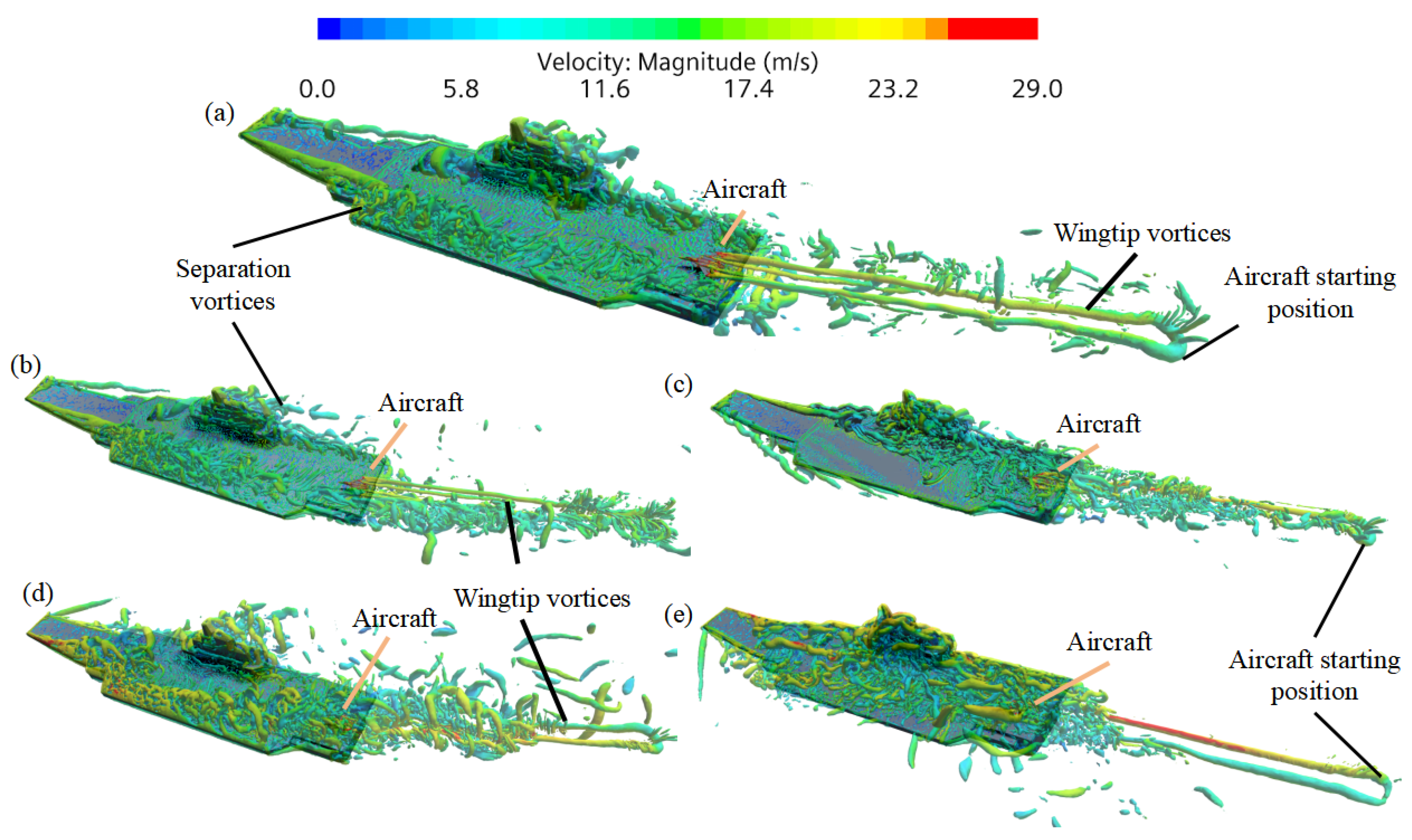
4.1. Aircraft Carrier Airwake

When the aircraft begins its landing approach, it encounters incoming airflow from various directions. The direction and magnitude of the airflow change continuously due to disturbances from the carrier’s hull. This section focuses on the impact of the airwake on the glideslope path and landing area of the aircraft. We emphasize the instantaneous state of the carrier’s wake field as the aircraft begins its approach. It takes the aircraft only 2.5 s to reach the deck from its starting position. Before the aircraft initiates its motion, the flow field state at this moment roughly corresponds to the airflow it is about to encounter.

Figure 9 depicts the velocity contours on the horizontal Section 5 m above the deck and the vertical section along the trajectory prior to the landing process. Figure 9a shows a slight downward deflection in the airflow direction at the stern of the carrier. This phenomenon is attributed to the Coanda effect, which causes the airflow passing over the deck to closely adhere to the surface, forming a downward wash airflow [34]. It is precisely this downward deflected airflow that leads to changes in the aircraft’s lift. During carrier navigation, it cannot be ensured that aircraft will always land with a headwind. The intensity and extent of the airwake vary significantly under different wind conditions. Figure 9b shows that the airflow flows smoothly at red 15° wind. At green 15° wind, due to disturbances from the carrier island on the right-hand side of the deck, there is noticeable turbulence at the stern. The stern exhibits a recirculation zone, but its influence extends below the deck plane as shown in Figure 9c. As the wind angle increases, the carrier island and deck edges exert stronger compression on the incoming airflow, resulting in a significant increase in local flow velocity. High-speed and low-speed regions alternate, and the velocity gradient within the space becomes greater. Upwash and downwash flows become more pronounced. At green and red 45° wind, as shown in Figure 9d,e, the change in flow direction within the range of 0~50 m from the stern becomes more pronounced. The circulation region extending from the stern exceeds the deck plane and enters the aircraft’s flight path.

To quantitatively predict the variable airflow along the aircraft’s flight path, the velocity profiles are extracted just before aircraft’s movement. Figure 10a shows the instantaneous velocity along the glideslope. At wind angles of 45°, the airflow fluctuates significantly more compared to 0° and 15° conditions due to the obstruction caused by the ship’s structure and superstructures.

To further demonstrate the influence of airwake turbulence on the trajectory, we analyze the flow characteristics of velocity components along the aircraft’s descent path. The airflow velocity is decomposed into three directional components based on GCS. Figure 10b shows that the x-direction velocity component displays fluctuation characteristics similar to the resultant velocity, particularly with enhanced variations near the hull region. Additionally, there are extended regions of low-speed flow, as observed in the vorticity and velocity contour plots, indicating burble separation from the hull. These clusters of low-speed regions tend to migrate downstream with the airflow. Figure 10c shows the component of velocity in the vertical direction. This component directly affects the AOA of the aircraft during flight, which ultimately influences the lift of the aircraft. The figure indicates that under different wind angles, a downwash region is formed at the stern of the carrier, with varying lengths and amplitudes. Under the conditions of 0° and red 15° wind, the vertical velocity changes relatively consistently. In these conditions, the airflow passes through the left side of the deck’s recovery runway, which results in a cleaner area with less turbulence. However, under other wind angle conditions, the airflow is disturbed by the edge of the deck and the island, leading to greater vertical fluctuations. Beyond a distance of 150 m from the stern, the vertical component of velocity tends towards stable. Figure 10d represents the lateral component of the velocity along the glideslope (positive towards the right). Within the range of −25 to −150 m from the stern, the direction of the lateral component is generally aligned with the incoming flow direction. At a distance of 25 m from the stern, the airflow begins to turn horizontally, indicating lateral recirculation near the hull. This causes a deviation in the sideslip angle during landing process. Furthermore, as the wind angle increases, the horizontal component of turning becomes more pronounced, ultimately resulting in greater variations in side force. In high-angle crosswinds, the deck contributes more to flow separation.

Overall, the analysis of flow characteristics along the approach line reveals a highly disturbed three-dimensional flow in the vicinity of the ship’s hull. As the airwake evolves, it moves downstream, creating an airwake effect that impacts aircraft during the landing process. By analyzing the velocity and its components along the approach line under the influence of the airwake, non-periodic fluctuations in the airflow are observed. These fluctuations cause the aircraft to experience significant variations in drag, lift, and side forces. However, given the aircraft’s length of 22 m and wingspan of 12 m, the data along the approach line alone are insufficient to fully characterize the flow field encountered by the aircraft. Therefore, the forces acting on the aircraft during its landing process have been computed.

4.2. Influence of Airwake on Aircraft Aerodynamic Loads

This section investigates the variations in forces acting on the aircraft during the landing process under different wind directions. Figure 11 shows the changes in the aircraft overset grids during the landing process, from the initial position to the final position. The aircraft approaches the carrier at a constant speed and AOA, eventually landing at the ideal touchdown point. As the aircraft approaches the hull, the bottom of the aircraft’s overset grid region extends beyond the deck into the computational domain exterior.

Figure 12 shows the merging Q-criterion of carrier airwake and aircraft airwake during landings under different wind angles. The isosurface of the Q-criterion clearly exhibits the locations of airflow separation and flow direction. The figures reveal that the carrier island, windward deck, rear edge of the deck and wingtips are the core regions where the airwake generates. At the starting position of the aircraft, wingtip vortices form a closed loop due to the initiation of aircraft motion. The wingtip vortices extend more than 150 m, combined with the carrier airwake, significantly impacting the handling performance of subsequent landing aircraft. The focus is on the distribution of vortices along the glideslope. Figure 12a,b reveal that under 0° and red 15° wind conditions, the area above the deck along the flight path appears relatively clean. Under green 15° wind conditions, the airwake extends farthest along the approach line, as shown in Figure 12c. At 45° wind angle condition, as the aircraft approaches the ship, its fuselage is submerged by the carrier’s airwake, as shown in Figure 12d,e.

Figure 13 is the lift variation during the landing process of the aircraft under different wind angles. To compare the impact of the airwake on the aircraft aerodynamic loads, we established a computational domain without the carrier. At the onset of the calculation, the aircraft remains at its initial position. After airflow passes through the entire computational domain, the aircraft begins its flight. The dashed line in the figure represents the variation of lift for the aircraft under the condition without the carrier. Under this condition, the lift of the aircraft remains nearly constant, with an average value of 2.16 × 10² kN, which is considered as the reference value. The magnitude of lift is close to the weight of the aircraft. The solid line represents the variation of lift for the aircraft with the presence of the carrier airwake, as shown in Figure 13a. Throughout the process, the lift fluctuates around the reference value. In the initial stage, the aircraft enters the region influenced by the carrier airwake. As it approaches the deck, the lift rapidly decreases. This region is the transition zone from upwash to downwash flow. The figure illustrates that when the wind direction aligns with the aircraft’s flight direction, the lift variation is most minimal. As the wind angle changes, fluctuations in lift occur within the 200 m before touchdown, characterized by multiple peaks and troughs throughout the process. As the aircraft approaches the carrier, there is a noticeable minimum point for lift. This minimum lift point occurs within a range of 100 m from the aft edge of the deck. Moreover, as the angle of the wind on the deck increases, the range of lift variation also increases. The decrease in lift within the stern area may lead to the aircraft deviating below the normal flight path, potentially resulting in a collision with the carrier’s stern. Moreover, this distance requires only 1 s for the aircraft to fly through. The instantaneous, nonlinear, and variable nature of the lift changes placea extremely high demands on the precision of the control system.

As the aircraft approaches directly above the deck (within 0 to 50 m), a sudden increase in lift is observed. Due to the aircraft’s hard landing, the descent rate is rapid. The compression of air between the fuselage, wings, and ground generates ground effect, leading to a rapid increase in lift. Under different wind direction conditions, an increasing trend in lift is observed, indicating that the ground effect predominates in the area above the deck. Figure 13b presents a statistical analysis of the aircraft lift range for two distinct flight phases. The first phase comprises approaching the deck (x = −150 to 0 m), and the second phase encompasses 50 m above the deck (x = 0 to 50 m). Here, the range is defined as the difference between maximum and minimum lift values. Results indicate the deck-crossing phase under ground effect produces markedly greater lift range variations compared to the approach phase subject to carrier airwake disturbances. The influence of airflow direction changes, airwake, and airflow separation on the fuselage is less significant compared to the ground effect. The increased lift in this area leads to a higher failure rate of the hook arresting cable.

The results reveal a contradiction throughout the entire approach and landing process. Near the carrier’s stern, the aircraft must maintain sufficient lift to avoid collision risks caused by lift reduction. However, before touchdown, lift must be reduced to ensure accurate engagement with the arresting cable, while increased lift complicates the hooking process. Therefore, resolving this contradiction demands precise and rapid flight control.

From the airflow analysis along the flight path in the previous section, it is evident that local downwash reduces the AOA, leading to a decrease in lift. Moreover, the situation is more complex for the entire fuselage. By comparing the aircraft lift variation curve with the velocity variation curve along the flight path under the influence of the carrier’s airwake, it is observed that the changes in aircraft lift do not fully correlate with the vertical velocity component. This discrepancy is attributed to varying airflow conditions, which cause differences in flow velocity and AOA at different sections of the fuselage.

Figure 14a shows the variation in drag during the aircraft carrier landing process. In the absence of carrier wake influence, aircraft drag force remains consistent, serving as a reference value. The graph indicates minimal drag force fluctuations at a wind angle of 0°, with increased fluctuations at other wind angles. Under different wind directions, the drag force values fluctuate around the reference value. As the aircraft approaches the touchdown point, the drag increases. This implies that the airwake near the ship’s hull contributes to higher flight drag. Figure 14b analyzes the drag range during two phases. Drag force variations grow significantly with wind angle in the airwake region. Above the deck, drag force fluctuations intensify further. This confirms that the ground effect remains dominant.

Through the carrier airwake velocity component curves, it is evident that the flow direction changes continuously, causing fluctuations in the aircraft’s sideslip angle during landing. Correspondingly, the aircraft’s side force also varies accordingly. Figure 15a depicts the changes in the aircraft’s side force. Shifts in the side force are observed as the aircraft approaches within 50 m of the stern. Moreover, with increasing wind angles, the changes in side force become more pronounced, potentially causing deviations from the intended flight path. As mentioned earlier, the analysis indicates the presence of a recirculation zone above the deck, resulting in a reversal of the side force direction just before reaching the touchdown point. Figure 15b presents the side force range during two phases. The results demonstrate that as wind angle increases, the recirculation around the hull significantly amplifies lateral force effects on the aircraft, surpassing even the ground effect influence.

The analysis above examines the forces acting on aircraft during landing under the influence of the carrier’s airwake. A comparison between the aircraft lift curve and the vertical component of the carrier airwake speed reveals a similar, but not perfectly aligned, trend. The velocity curve of the carrier’s airwake alone cannot fully reflect the changes in force acting on the aircraft during landing. There are several reasons for this discrepancy. Firstly, the aircraft is a three-dimensional object that occupies a certain space in terms of length and wingspan. There are differences in local airspeed and AOA between the left and right wings. Additionally, the velocity depicted in Figure 12 represents the flow field information at the moment just before the aircraft’s passage. It takes some time for the aircraft to enter this segment of the flight path, during which the flow conditions along the trajectory have changed. As the aircraft approaches and enters the area above the deck, the ground effect becomes the dominant factor. Studying the carrier’s airwake alone cannot comprehensively reveal the effects produced by the ground effect. The instantaneous velocity prediction on the carrier’s airwake qualitatively reflects the flight conditions that the aircraft will encounter, but it is insufficient for predicting the aircraft’s aerodynamic loads. Therefore, comprehensive analysis must integrate both the carrier airwake flow field and coupled aircraft–carrier dynamics in the simulation.

Analysis of the forces acting on the aircraft in three dimensions reveals that the magnitude of forces differs by an order of magnitude in each direction, indicating that the lift significantly exceeds the drag and side forces. Furthermore, the variations in forces throughout the flight process highlight the aircraft’s sensitivity to longitudinal airflow disturbances. The following section examines the amplification of airwake disturbances by ship vertical motion and its subsequent impact on aircraft lift variation.

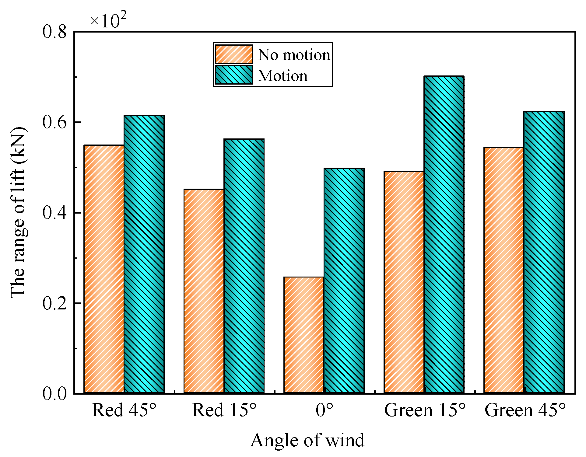
4.3. Influence of the Airwake on the Lift Under Ship Motion

In actual sea conditions, ships undergo six degrees of freedom motion due to the effects of waves and wind. The motion of the hull enhances the disturbance of the airwake. The authors of [21] conducted a comprehensive analysis of three ship motion components (heave, roll, and pitch). Given that heave and pitch exhibit significantly larger vertical displacements and greater wake disturbances compared to other degrees of freedom, this section focuses on these two dominant motions in the vertical plane. The axis of the ship’s pitching motion aligns with the z-axis of the CCS. The motion law of the ship follows [35]

$$h=1.22\sin (0.6t)+0.3\sin (0.23t)$$

(19)

$$\psi =0.5\sin (0.6t)+0.3\sin (0.63t)$$

(20)

where h represents location of the heave motion, and ψ represents the angle of pitch.

Given the predetermined carrier motion profile and fixed aircraft approach parameters, the carrier’s landing position is computed in advance. This allows precise adjustment of the aircraft’s initial altitude to ensure touchdown at the designated deck position.

Before the aircraft moves, the flow field information along the glideslope is extracted, with a focus on the vertical velocity component. Figure 16 shows the velocity and vertical component along the glideslope when the carrier undergoes two degrees of freedom motion. Near the edge of the deck, at approximately 100 m, velocity fluctuations intensify. Compared to the stationary carrier condition, fluctuations in the vertical component are significantly amplified. The range between the highest and lowest values is greater than that under stationary carrier conditions. The large velocity gradient within the last 100 m before reaching the deck results in more complex landing conditions.

The degree of airflow disturbance within the flow field is quantitatively described by turbulence intensity (Ti). Its definition is the root-mean-square of the fluctuating velocity divided by the free-stream velocity.

$$Ti={\displaystyle \frac{\sqrt{\frac{1}{3}\left({u^{\prime }}^2+{v^{\prime }}^2+{w^{\prime }}^2\right)}}{U_{\infty }}}$$

(21)

where u′, v′, and w′ represent the fluctuating velocities in the u, v, and w velocity components, respectively. U_∞ represents the free-stream velocity.

Figure 17 shows Ti values along the glideslope under stationary and moving hull conditions, respectively. Consistent with velocity fluctuations, Ti begins to increase within 100 m of the deck, reaching its maximum directly above the deck. As the wind angle increases, Ti also increases. It indicates that not only the ship island but also the flat deck edges induce flow separation and contribute to higher Ti. Disturbances generated by winds on the starboard side are greater than those on the port side, suggesting that the prominent ship island induces stronger disturbances. It is evident that Ti values in Figure 17b significantly exceed those in Figure 17a. This phenomenon demonstrates the magnifying effect of hull movement on airflow turbulence.

Figure 18 depicts the lift variation during aircraft landing under hull motion. Figure 19 compares the range of lift within −150 to 0 m, excluding the phase above the deck, under stationary and moving hull conditions. It is observed that when the hull is in motion, there is a greater range of lift during the landing process. The hull’s longitudinal motion, including heave and pitch, increases turbulence intensity and exacerbates flow separation, ultimately leading to larger fluctuations in aircraft lift.

Figure 18 shows that the minimum lift occurs within 0 to −50 m before reaching the deck. Moreover, the minimum lift value is lower than that under stationary conditions. This phase is critical just before landing, as a sudden decrease in lift at this point may lead to an early touchdown. In severe cases, it may result in the aircraft colliding with the stern of the carrier. Furthermore, under hull motion conditions, the lift increases more rapidly after the aircraft flies over the deck, making it more difficult to engage the arresting cable.

In reality, the motion of the hull not only intensifies the turbulence of the airwake, leading to a lager range of lift fluctuations but also complicates the identification of the touchdown point. The flight control system must continuously monitor different parameters of the aircraft and make adjustments based on the real-time conditions. The environmental changes induced by hull motion require the flight control system to process more information, further increasing the workload of both the system and the pilots.

5. Conclusions

The unsteady numerical simulation accurately resolves the transient airwake field generated by the aircraft carrier. However, predicting the ship’s airwake only partially reflects the impact of airflow, as it does not align with the forces acting on the aircraft. Therefore, a unified dynamic model integrating the ship and aircraft was constructed to compute the aerodynamic loads during carrier landing. Polyhedral grids are well-suited for modeling the complex geometries of both the carrier and aircraft. The use of DDES-overset grid coupling ensures numerical stability during the aircraft landing process. The dual-overset grid method is employed to analyze coupled carrier–aircraft dynamics, capturing airwake disturbances enhanced by carrier heave and pitch motions. The study analyzes the effect of airflow turbulence on the aircraft’s aerodynamic loads under varying wind angles, resulting in the following conclusions:

(1)

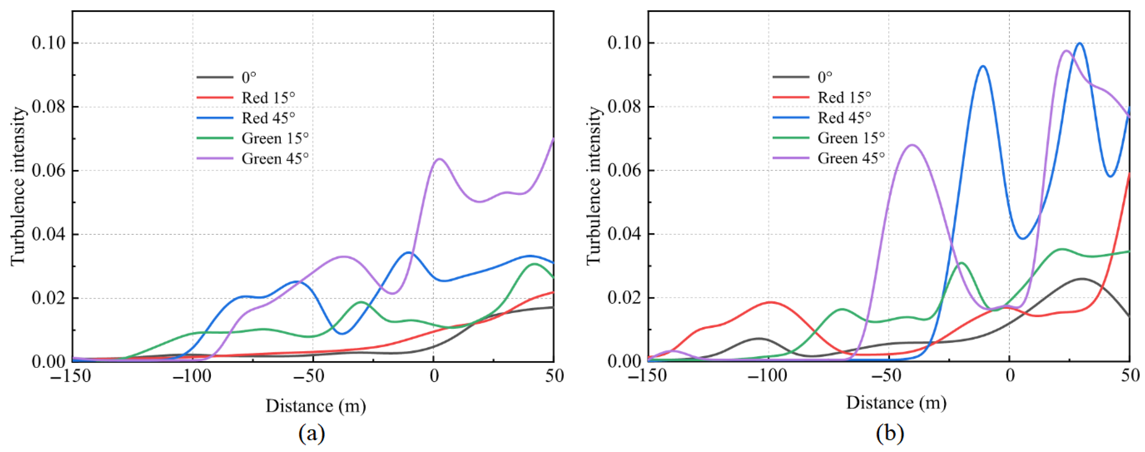
The airflow around the aircraft carrier undergoes significant disturbance due to the carrier’s structure. Upwash, downwash, and lateral transition zones were identified within 150 m of the carrier’s hull.

(2)

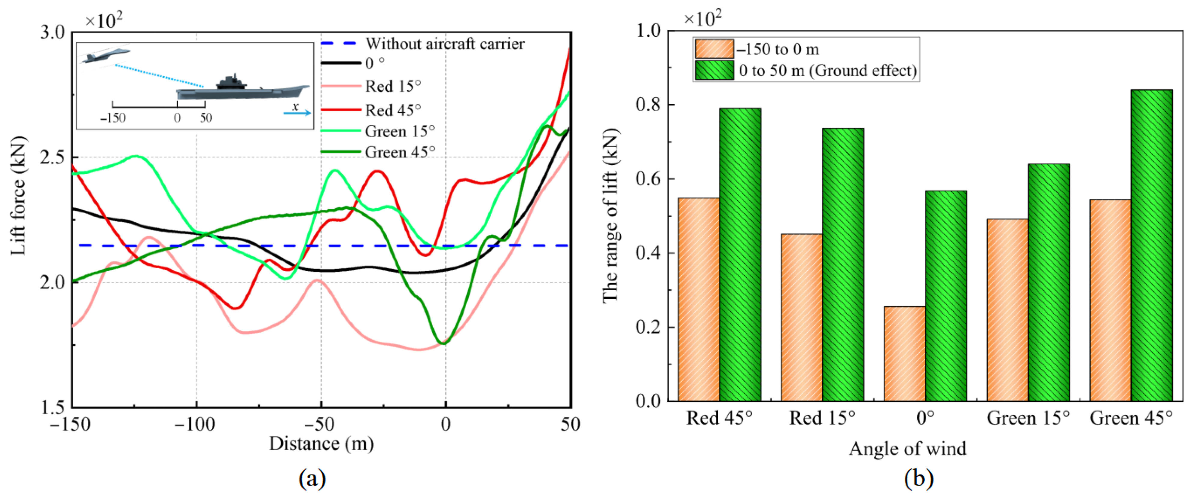
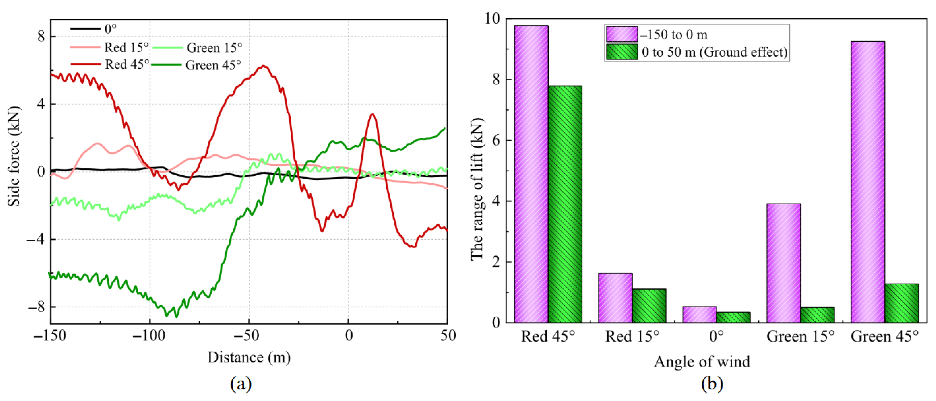
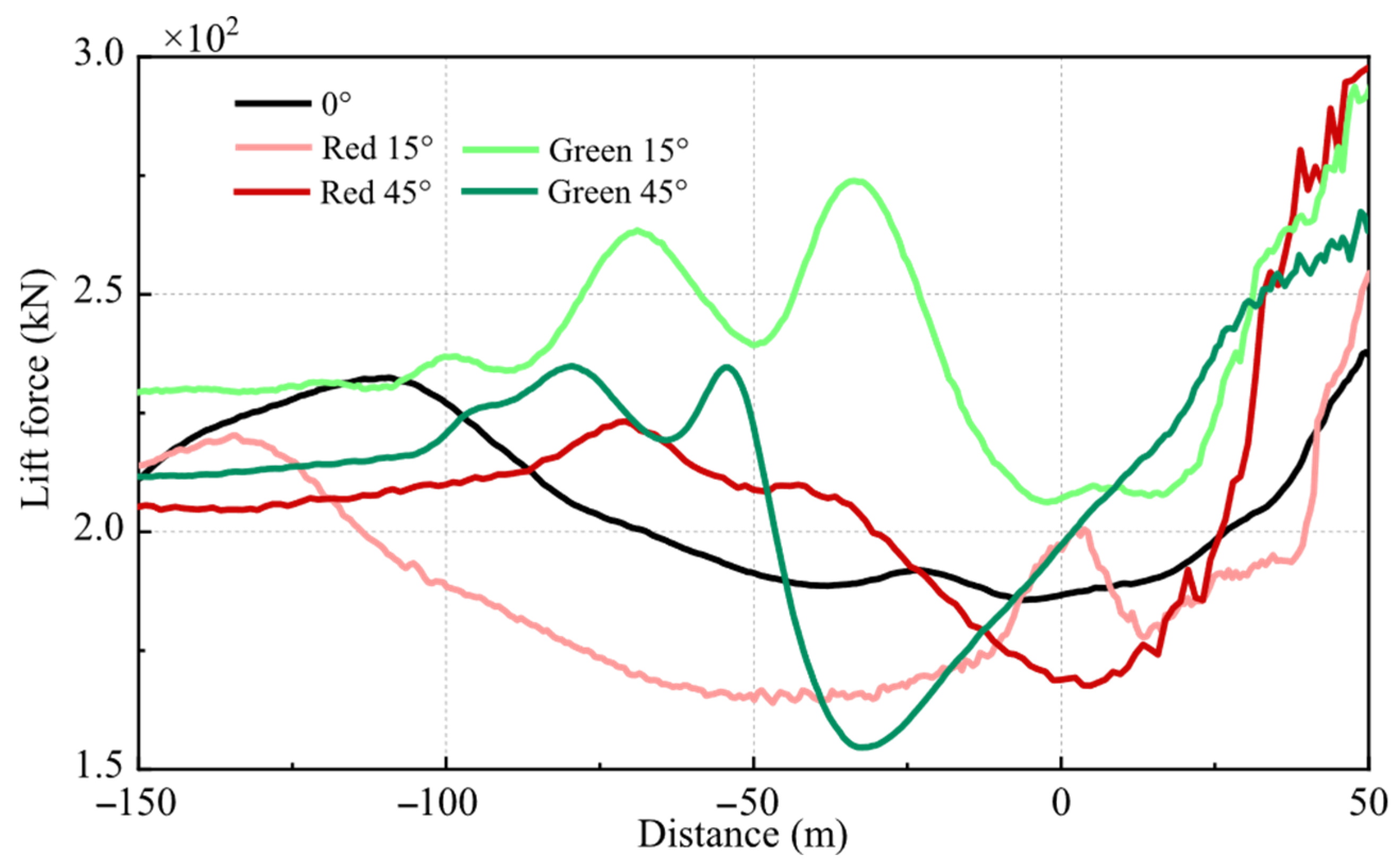
The trends in aircraft lift and side force variations closely resemble the airwake variations along the glideslope in the airwake but are not entirely consistent. The minimum aircraft lift occurs within 100 m of the stern, where a sudden decrease in lift could increase the risk of collision with the hull. As the wind angle increases, the aircraft drag rises, further intensifying as the aircraft approaches the hull. Additionally, during the aircraft’s approach to the hull, the side forces reverse direction, with larger wind angles generating greater turning forces.

(3)

Above the deck, the aircraft’s forces are predominantly influenced by the ground effect. As the aircraft approaches the deck, a sharp increase in lift occurs, potentially increasing the failure rate of the arresting cable hook.

(4)

The hull’s vertical motion intensifies the turbulence intensity of the airwake, ultimately resulting in a wider range of aircraft lift values during the landing process.

These findings provide valuable insights for improving carrier-based aircraft recovery procedures, offering more realistic data for simulation training and helping pilots better prepare for airwake-induced disturbances.

References

1. Zamiri, A.; Chung, J.T. Numerical evaluation of wind direction effects on the turbulence aerodynamics of a ship airwake. Ocean. Eng. 2023, 284, 115104. [Google Scholar] [CrossRef]
2. Cherry, B.E.; Constantino, M.M. The Burble Effect Superstructure and Flight Deck Effects on Carrier Air Wake. In Proceedings of the American Society of Naval Engineers Launch and Recovery Symposium, Arlington, VA, USA, 8–9 December 2010; United States Naval Academy: Annapolis, MD, USA, 2010. [Google Scholar]
3. Shukla, S.; Sinha, S.S.; Singh, S.N. Ship-helo coupled airwake aerodynamics: A comprehensive review. Prog. Aerosp. Sci. 2019, 106, 71–107. [Google Scholar] [CrossRef]
4. Bardera, R.; Barcala-Montejano, M.A.; Rodríguez-Sevillano, A.A.; León-Calero, M. Wind flow investigation over an aircraft carrier deck by PIV. Ocean. Eng. 2019, 178, 476–483. [Google Scholar] [CrossRef]
5. Owen, I.; Lee, R.; Wall, A.; Fernandez, N. The NATO generic destroyer—A shared geometry for collaborative research into modelling and simulation of shipboard helicopter launch and recovery. Ocean Eng. 2021, 228, 108428. [Google Scholar] [CrossRef]
6. Setiawan, H.; Kevin; Philip, J.; Monty, J.P. Turbulence characteristics of the ship air-wake with two different topside arrangements and inflow conditions. Ocean Eng. 2022, 260, 111931. [Google Scholar] [CrossRef]
7. Shukla, S.; Singh, S.; Sinha, S.; Vijayakumar, R. Vijayakumar, Comparative assessment of URANS, SAS and DES turbulence modeling in the predictions of massively separated ship airwake characteristics. Ocean Eng. 2021, 229, 108954. [Google Scholar] [CrossRef]
8. Shipman, J.; Arunajatesan, S.; Menchini, C.; Sinha, N. Ship Airwake Sensitivities To Modeling Parameters. In Proceedings of the 43rd AIAA Aerospace Sciences Meeting and Exhibit, Reno, NV, USA, 10–13 January 2005. [Google Scholar]
9. Thornber, B.; Starr, M.; Drikakis, D. Implicit Large Eddy Simulation of Ship Airwakes. Aeronaut. J. 2010, 114, 715–736. [Google Scholar] [CrossRef]
10. Spalart, P.R. Comments on the feasibility of LES for wings, and on a hybrid RANS/LES approach. In Proceedings of the First AFOSR International Conference on DNS/LES, Ruston, LA, USA, 4–8 August 1997. [Google Scholar]
11. Spalart, P.R.; Deck, S.; Shur, M.L.; Squires, K.D.; Strelets, M.K.; Travin, A. A new version of detached-eddy simulation, resistant to ambiguous grid densities. Theor. Comput. Fluid Dyn. 2006, 20, 181–195. [Google Scholar] [CrossRef]
12. Forrest, J.S.; Owen, I. An investigation of ship airwakes using Detached-Eddy Simulation. Comput. Fluids 2010, 39, 656–673. [Google Scholar] [CrossRef]
13. Watson, N.A.; Kelly, M.F.; Owen, I.; Hodge, S.J.; White, M.D. Computational and experimental modelling study of the unsteady airflow over the aircraft carrier HMS Queen Elizabeth. Ocean Eng. 2019, 172, 562–574. [Google Scholar] [CrossRef]
14. Kelly, M.F.; White, M.; Owen, I.; Hodge, S.J. Using airwake simulation to inform flight trials for the Queen Elizabeth Class Carrier. In Proceedings of the 13th International Naval Engineering Conference, INEC 2016, Bristol, UK, 26–28 April 2016. [Google Scholar]
15. Nisham, A.; Terziev, M.; Tezdogan, T.; Beard, T.; Incecik, A. Prediction of the aerodynamic behaviour of a full-scale naval ship in head waves using Detached Eddy Simulation. Ocean Eng. 2021, 222, 108583. [Google Scholar] [CrossRef]
16. Yang, X.; Li, B.; Ren, Z.; Tian, F. Numerical Simulation of the Unsteady Airwake of the Liaoning Carrier Based on the DDES Model Coupled with Overset Grid. J. Mar. Sci. Eng. 2024, 12, 1598. [Google Scholar] [CrossRef]
17. Shipman, J.; Cavallo, P.; Arunajatesan, S.; Sinha, N. Dynamic CFD Simulation of Aircraft Recovery to an Aircraft Carrier. In Proceedings of the 26th AIAA Applied Aerodynamics Conference, Honolulu, HI, USA, 18–21 August 2008. [Google Scholar]
18. Lee, D.; Sezer-Uzol, N.; Horn, J.F.; Long, L.N. Simulation of helicopter shipboard launch and recovery with time-accurate airwakes. J. Aircr. 2005, 42, 448–461. [Google Scholar] [CrossRef]
19. Kääriä, C.H.; Wang, Y.; Padfield, G.D.; Forrest, J.S.; Owen, I. Aerodynamic Loading Characteristics of a Model-Scale Helicopter in a Ship’s Airwake. J. Aircr. 2012, 49, 1271–1278. [Google Scholar] [CrossRef]
20. Forrest, J.S.; Owen, I.; Padfield, G.D.; Hodge, S.J. Ship-Helicopter Operating Limits Prediction Using Piloted Flight Simulation and Time-Accurate Airwakes. J. Aircr. 2012, 49, 1020–1031. [Google Scholar] [CrossRef]
21. Watson, N.A.; Owen, I.; White, M.D. Piloted Flight Simulation of Helicopter Recovery to the Queen Elizabeth Class Aircraft Carrier. J. Aircr. 2020, 57, 742–760. [Google Scholar] [CrossRef]
22. Bridges, D.; Horn, J.; Alpman, E.; Long, L. Coupled Flight Dynamics and CFD Analysis of Pilot Workload in Ship Airwakes. In Proceedings of the AlAA Atmospheric FlightDynamics Conference, Hilton Head, SC, USA, 20–23 August 2007. [Google Scholar]
23. Kääriä, C.H.; Wang, Y.; White, M.D.; Owen, I. An experimental technique for evaluating the aerodynamic impact of ship superstructures on helicopter operations. Ocean. Eng. 2013, 61, 97–108. [Google Scholar] [CrossRef]
24. Forrest, J.; Kaaria, C.; Owen, I. Evaluating ship superstructure aerodynamics for maritime helicopter operations through CFD and flight simulation. Aeronaut. J. 2016, 120, 1578–1603. [Google Scholar] [CrossRef]
25. Shi, Y.; Su, D.; Xu, G. Numerical investigation of the influence of passive/active flow control on ship/helicopter dynamic interface. Aerosp. Sci. Technol. 2020, 106, 106205. [Google Scholar] [CrossRef]
26. Su, D.; Xu, G.; Huang, S.; Shi, Y. Numerical investigation of rotor loads of a shipborne coaxial-rotor helicopter during a vertical landing based on moving overset mesh method. Eng. Appl. Comput. Fluid Mech. 2019, 13, 309–326. [Google Scholar] [CrossRef]
27. Dooley, G.M.; Carrica, P.; Martin, J.; Krebill, A.; Buchholz, J. Effects of Waves, Motions and Atmospheric Turbulence on Ship Airwakes. In Proceedings of the AIAA Scitech 2019, San Diego, CA, USA, 7–11 January 2019. [Google Scholar]
28. Dooley, G.; Martin, J.E.; Buchholz, J.H.; Carrica, P.M. Ship Airwakes in Waves and Motions and Effects on Helicopter Operation. Comput. Fluids 2020, 208, 104627. [Google Scholar] [CrossRef]
29. Thedin, R.; Kinzel, M.P.; Horn, J.F.; Schmitz, S. Coupled Simulations of Atmospheric Turbulence-Modified Ship Airwakes and Helicopter Flight Dynamics. J. Aircr. 2019, 56, 812–824. [Google Scholar] [CrossRef]
30. Thedin, R.; Murman, S.M.; Horn, J.; Schmitz, S. Effects of Atmospheric Turbulence Unsteadiness on Ship Airwakes and Helicopter Dynamics. J. Aircr. 2020, 57, 534–546. [Google Scholar] [CrossRef]
31. Menter, F.R.; Kuntz, M.; Langtry, R. Ten years of industrial experience with the SST turbulence model, Turbulence. Heat Mass Transf. 2003, 4, 625–632. [Google Scholar]
32. Zhang, J.; Minelli, G.; Rao, A.N.; Basara, B.; Bensow, R.; Krajnović, S. Comparison of PANS and LES of the flow past a generic ship. Ocean Eng. 2018, 165, 221–236. [Google Scholar] [CrossRef]
33. Ladson, C. Effects of Independent Variation of Mach and Reynolds Numbers on the Low-Speed Aerodynamic Characteristics of the NACA 0012 Airfoil Section. In Proceedings of the NASA Langley Research Center, NASA Technical Memorandum 4074, Hampton, VA, USA, 23 August 1988. [Google Scholar]
34. Xu, K.; Su, X.; Bensow, R.; Krajnovic, S. Large eddy simulation of ship airflow control with steady Coanda effect. Phys. Fluids 2023, 35, 015112. [Google Scholar] [CrossRef]
35. Li, X. Simulation of Key Technology of Lanuch and Land for Carrier-Based Aircraft; Harbin Engineering University: Harbin, China, 2012; pp. 23–25. [Google Scholar]
Figure 1. Schematic diagram of overset grids: (a) overset grids for single-body motion, (b) overset grids for dual-body motion.
Aerospace 12 00656 g001
Figure 2. Schematic diagram of the geometry models and boundary conditions: (a) geometry models of the aircraft carrier and the aircraft, (b) boundary conditions for the entire computational domain, and (c) the boundary conditions for the aircraft engines.
Aerospace 12 00656 g002
Figure 3. Velocity decomposition diagram of the aircraft landing process.
Aerospace 12 00656 g003
Figure 4. Grids of the computational domain: (a) independent grid regions, (b) internal grids of each region, and (c) grids of the critical segments.
Aerospace 12 00656 g004
Figure 5. Grid independence validation.
Aerospace 12 00656 g005
Figure 6. Schematic of NACA0012 airfoil profile for validation.
Aerospace 12 00656 g006
Figure 7. Mesh of NACA0012 airfoil profile.
Aerospace 12 00656 g007
Figure 8. Comparisons of validation results: (a) lift coefficient, (b) drag coefficient.
Aerospace 12 00656 g008
Figure 9. Velocity contours on the horizontal section 5 m above the deck and the vertical section along the trajectory under a different wind direction: (a) headwind 0°, (b) red 15°, (c) green 15°, (d) red 45°, (e) green 45° (Left: Top view, right: side view). Green denotes the starboard (right) wind direction, while red denotes the port (left) direction.
Aerospace 12 00656 g009
Figure 10. Velocity and velocity components along the glideslope: (a) velocity, (b) u component, (c) v component, (d) w component.
Aerospace 12 00656 g010
Figure 11. The overset grid dynamic location: (a) the initial location of aircraft, (b) the touchdown location of aircraft.
Aerospace 12 00656 g011
Figure 12. Isosurface of Q-criterion colored by velocity during aircraft landing phase under different wind angles: (a) 0°, (b) red 15°, (c) green 15°, (d) red 45°, (e) green 45°.
Aerospace 12 00656 g012
Figure 13. Variation in aircraft lift under the influence of aircraft carrier airwake under different wind angles, (a) variation in aircraft lift, and (b) range of lift.
Aerospace 12 00656 g013
Figure 14. Variation in drag force under different wind angles, (a) variation in drag force, (b) and range of drag force.
Aerospace 12 00656 g014
Figure 15. Variation in aircraft side force under different wind angles, (a) variation in side force, and (b) range of side force.
Aerospace 12 00656 g015
Figure 16. Velocity and vertical velocity components along the glideslope with ship heave and pitch motion, (a) velocity, and (b) v component.
Aerospace 12 00656 g016
Figure 17. Turbulence intensity along the glideslope (a) with stationary hull and (b) with hull heave and pitch motion.
Aerospace 12 00656 g017
Figure 18. Variation in aircraft lift under the influence of aircraft carrier airwake with hull heave and pitch.
Aerospace 12 00656 g018
Figure 19. The range of aircraft lift under with hull motion and without motion.
Aerospace 12 00656 g019