A CAD-Based Method for 3D Scanning Path Planning and Pose Control

Abstract

To address the technical bottlenecks of low path planning efficiency and insufficient point cloud coverage in the automated 3D scanning of complex structural components, this study proposes an offline method for the generation and optimization of scanning paths based on CAD models. Discrete sampling of the model’s surface is achieved through the construction of an oriented bounding box (OBB) and a linear object–triangular mesh intersection algorithm, thereby obtaining a discrete point set of the model. Incorporating a standard vector analysis of the discrete points and the kinematic constraints of the scanning system, a scanner pose parameter calculation model is established. An improved nearest neighbor search algorithm is employed to generate a globally optimized scanning path, and an adaptive B-spline interpolation algorithm is applied to path smoothing. A joint MATLAB (R2023b)—RobotStudio (6.08) simulation platform is developed to facilitate the entire process, from model pre-processing and path planning to path verification. The experimental results demonstrate that compared with the traditional manual teaching methods, the proposed approach achieves a 25.4% improvement in scanning efficiency and an 18.6% increase in point cloud coverage when measuring typical complex structural components. This study offers an intelligent solution for the efficient and accurate measurement of large-scale complex parts and holds significant potential for broad engineering applications.

1. Introduction

With the continuous advancement of industrial demands for higher manufacturing accuracy and quality, especially in the inspection of complex-shaped and large-scale components, the traditional manual measurement methods are increasingly becoming inadequate to meet the requirements of digital manufacturing [1]. Although digital measurement technologies are gaining traction, photogrammetry remains limited in accuracy, and coordinate measuring machines (CMMs) lack the efficiency required for large-scale production [2]. In response, many domestic manufacturing enterprises have adopted three-dimensional laser scanning—a high-precision, non-contact, and rapid data acquisition technology—to support quality inspection, reverse engineering, and digital manufacturing of complex structural components [3]. This technology enables the rapid acquisition of high-density surface point clouds, offering a reliable basis for downstream CAD modeling and analysis. Integrating industrial robots with 3D laser scanning systems facilitates automated scanning and digital manufacturing of structural components. However, scanning path planning for complex structural components still faces numerous challenges: the traditional methods are heavily reliant on manual intervention, resulting in low efficiency and a suboptimal point cloud quality that often fails to meet the precision requirements [4,5]. Therefore, the development of automated path planning strategies to enhance the scanning efficiency and point cloud reconstruction accuracy has become an urgent research priority.

In recent years, three-dimensional (3D) scanning path planning has emerged as a research hotspot in the field of laser scanning technology. Numerous studies conducted by international researchers have proposed a variety of path optimization strategies and achieved notable progress. For instance, Maskeliūnas et al. [6] developed a LiDAR–photogrammetry data fusion framework aiming to enhance the 3D scanning accuracy and improve the detection efficiency. However, due to the large size of complex structural parts, it remains difficult to ensure measurement accuracy despite improvements in efficiency. Han [7] proposed the COSPS method, which enhances the 3D path planning efficiency and reduces complexity by analyzing key obstacles and neighboring point sets. Sun et al. [8] introduced a path generation strategy based on STL models, optimizing the path spacing and scanning angles to improve both efficiency and accuracy. Huang et al. [9] investigated a B-spline-based path smoothing technique, where adjusting the control point positions effectively reduced the maximum curvature and improved the system’s processing quality. Lian et al. [4] proposed a discontinuous meshing-based algorithm capable of automatically generating adaptive scanning paths for large-scale complex geometries, significantly enhancing the scanning efficiency. Song [10] applied an adaptive ant colony optimization algorithm combined with fuzzy logic to 3D scanning path planning, thereby improving the measurement accuracy. Wang et al. [11] presented a deep-neural-network-enhanced sampling path planning method that accelerated scanning by predicting potential path regions. Liu et al. [12] introduced a tangent-graph-based UAV path planning approach capable of avoiding obstacles in low-altitude urban environments while ensuring efficient navigation. Wang et al. [13] proposed a load-transmission-based path planning strategy to improve the mechanical properties of continuous fiber-reinforced composites. Anagnostakis et al. [14] explored a measurement method using coordinate measuring machines (CMMs), acquiring data after precise part positioning but without addressing path planning. While the research in China began relatively late, it has progressed rapidly in recent years. Zhao et al. [15] employed Motosim (2018) software for offline robot programming to generate automated measurement routines, enabling scanning-based inspections of components, although manual editing was still required. Gao et al. [16] guided a CMM using imported CAD models in PC-DMIS for automatic contact measurement, yet the approach remained inefficient. Ai et al. [17,18] developed an automated scanning system composed of a tracker, a scanner, a machine tool, and scanning software, enabling point cloud acquisition of structural parts. Zhou [19] proposed a pose optimization method for scanning path planning, contributing to further advancements in system integration and path accuracy.

In summary, although significant progress has been made in the field of 3D scanning path planning, challenges remain in terms of planning efficiency, algorithmic complexity, and scanning accuracy. For large components with complex geometries, the existing methods struggle to achieve automatic feature adaptation, often rely heavily on manual intervention, and lack the necessary flexibility and efficiency—making them inadequate to meet the stringent demands of modern manufacturing in terms of high-precision and high-efficiency inspections. To address critical bottlenecks such as low path planning efficiency and insufficient point cloud coverage, this study proposes an offline automatic scanning path generation and optimization method based on CAD models. First, by constructing an optimal oriented bounding box (OBB) and employing a linear object–triangular patch intersection algorithm, effective discretization of the complex surface model is achieved, resulting in a high-quality discrete point set. Subsequently, a multi-degree-of-freedom scanner pose estimation model is established by incorporating a standard vector analysis of the points and the kinematic constraints of the scanning system. During path generation, an improved nearest neighbor search algorithm is utilized to compute a globally optimized scanning path. In contrast, an adaptive B-spline interpolation algorithm is applied to enhancing the path’s smoothness and feasibility. A co-simulation platform based on MATLAB (R2023b) and RobotStudio (6.08) is developed, establishing a complete technical loop from model pre-processing and path planning to virtual validation. This integrated framework offers an intelligent and efficient path planning solution for automated 3D scanning of large-scale, geometrically complex structural components.

This study aims to develop an automatic scanning path generation and pose control method tailored to complex, curved structural components, addressing key challenges in the current 3D measurement processes for high-end manufacturing—namely, the reliance on manual experience for path planning, limited measurement coverage, and discontinuous pose adjustment. Unlike previous studies focused solely on algorithmic optimization or hardware development, our work emphasizes a system-level deployment strategy that can be generalized across different scanning setups while ensuring a high surface coverage and robust pose control. The ultimate goal is to improve the accuracy, efficiency, and stability of digitization processes for industrial parts and to provide a non-contact, high-precision, and automated 3D reconstruction solution adaptable to aerospace and other high-end manufacturing sectors.

Studying offline automatic 3D scanning path generation based on a CAD model of the target workpiece holds significant value in enhancing both the detection efficiency and measurement accuracy. On the one hand, this method facilitates the advancement of intelligent manufacturing by enabling a high degree of automation in the inspection process. On the other hand, efficient path planning reduces measurement redundancy, shortens detection times, and minimizes the errors associated with manual interventions, thereby improving the overall stability and reliability of the measurement workflow. More importantly, the research outcomes are applicable to the manufacturing of large-scale complex structural components with high-precision requirements—such as those in the aerospace, automotive, marine, and energy sectors—and offer robust technical support for three-dimensional measurements of intricate workpieces.

2. Composition of the Three-Dimensional Scanning System and the Path Planning Strategy

Aiming to address challenges in three-dimensional measurement such as complex part geometries, significant curvature variations, and reliance on manual experience for pose adjustments, this study proposes and implements a path planning and pose coordination strategy based on an existing measurement system consisting of a MetraSCAN 3D laser scanner and an industrial robot. The proposed strategy addresses core issues including field-of-view limitations, incident angle constraints, and dynamic tracking stability. Without modifying the system hardware, it establishes an automated 3D data acquisition workflow suitable for complex surface structures, enhancing both the data coverage and scanning efficiency. This section provides a systematic introduction to the system’s principles, constraint modeling, and the path generation methodology.

2.1. Composition of the Three-Dimensional Scanning Measurement System

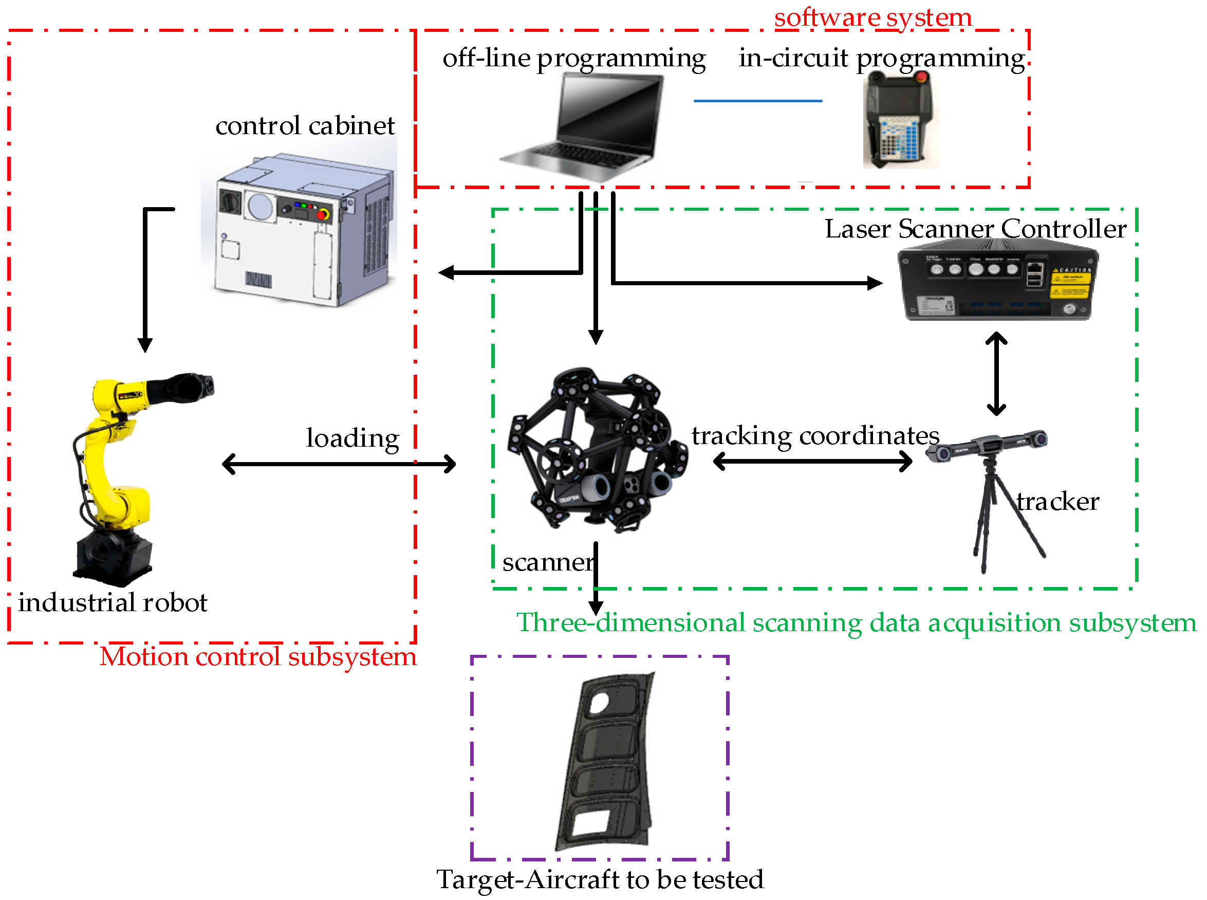
As illustrated in Figure 1, the automatic tracking 3D scanning measurement system, based on a laser 3D scanner and an industrial robot, comprises three primary subsystems:

(1) A 3D Scanning Data Acquisition Subsystem: This module includes a 3D scanning head and a laser positioning tracker, responsible for capturing high-precision point cloud data on the workpiece surface. (2) A Motion Control Subsystem: Composed of a six-degree-of-freedom industrial robot (scanning robot) and associated safety protection devices, this subsystem enables flexible operation within a trapezoidal workspace defined by the laser positioning system. It guides the scanning head to perform full-surface inspections of the components autonomously. (3) The Software System: This includes automatic scanning and detection software, as well as system control software, which collectively manage scanning path planning, execution commands, and data processing and storage. Within this system, the industrial robot manipulates the 3D scanning head throughout the workspace constrained by the tracking system, enabling high degrees of freedom in motion and supporting autonomous path programming and task scheduling. This integrated approach not only substantially expands the scanning area coverage but also enhances the measurement efficiency and elevates the automation level of the manufacturing inspection process.

As illustrated in Figure 1, the MetraSCAN 3D laser scanner integrates a central laser emitter and a high-resolution cameras on both sides, enabling efficient acquisition of large-scale, high-precision point cloud data. The key technical specifications are listed in

Table 1. MetraSCAN 3D scanning parameters.

Precision (mm)	Resolution (mm)	Baseline Distance L (mm)	Scanning Area A × B (mm)	Measurement Rate r (s)
0.02	0.05	300	275 × 250	1,800,000

. Based on triangulation and reflective marker tracking, the system reconstructs the spatial pose of the scanner in real time, facilitating fast and accurate 3D contour acquisition and modeling. The 3D scanning system employed in this study is based on the MetraSCAN 3D laser scanner (Creaform Inc., Lévis, QC, Canada), which is a high-precision, non-contact optical measurement device.

The optical tracking system illuminates reflective markers on the scanner using infrared beams to perform spatial positioning. By continuously capturing the 3D positions of these markers and applying calibration data, the system calculates the scanner’s pose with high accuracy throughout the scanning process. The measurement volume is defined as a trapezoidal region, as shown in Figure 2.

Although the system is built upon standard commercial equipment, this study proposes an integrated scanning deployment strategy tailored to complex surface components. The control scheme is designed through coordinated optimization of the industrial robot’s multi-degree-of-freedom motion, the scanning field-of-view limitations, and the requirements for 3D measurement accuracy. By integrating laser scanning, trajectory planning, and real-time pose correction into a unified workflow, the system exhibits strong potential for automated, high-coverage, and stable acquisition of data on complex components. This coordinated deployment is not a built-in feature of the commercial system but a custom-designed integration and control logic based on the specific demands of the measurement scenarios, showcasing the innovation of this work in functional-level deployment and modularized control design.

2.2. The System’s Scanning Principles and Acquisition Rules

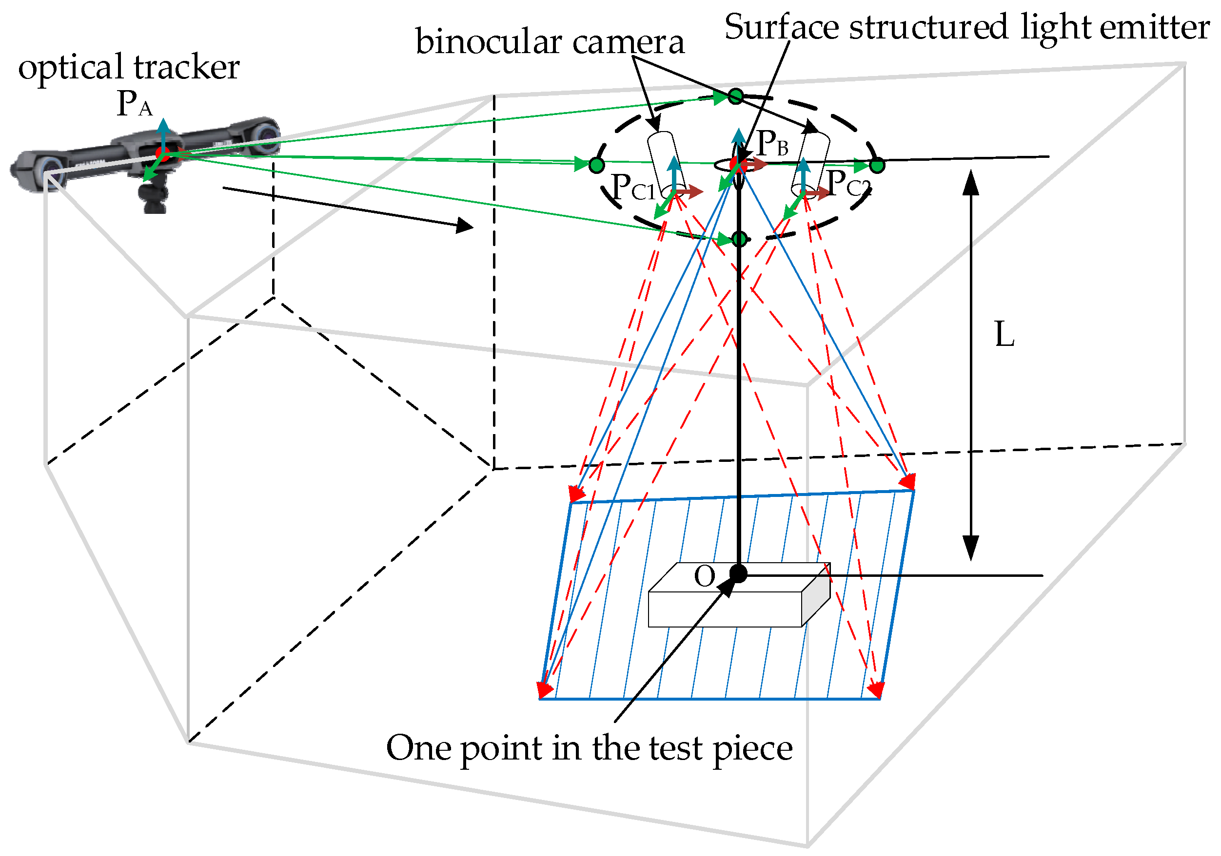
The scanning principle of the automated detection system for complex part geometries is illustrated in Figure 3. In this system, the 3D laser scanner is responsible for acquiring point cloud data from the target surface. At the same time, the optical tracker provides real-time measurements of the scanner’s three-dimensional position and orientation within the measurement space. The integration of these two subsystems enables the scanner’s spatial pose in the measurement coordinate system to be accurately determined. The coordinate system of the 3D scanning head is denoted as $P_B$. During scanning, the laser emitter projects rays onto the surface of the object under inspection, and the shape of the laser line dynamically changes according to the object’s surface contour. Utilizing a binocular camera system, the scanner captures the 3D coordinates of the laser-illuminated points on the object’s surface. For instance, point $O$ lies on the measured surface, with a distance $L$ from the laser emission point. The red laser line in the figure represents the scanning coverage region. The optical tracking system defines its coordinate system as $P_A$ and employs reflective marker tracking technology to acquire the spatial coordinates of each target on the scanning head at a frequency of 60 Hz. Finally, based on the phase measurement principle, the system computes the precise pose of each reflective target within the workspace, thereby achieving stable and continuous dynamic tracking of the scanning probe.

If ${}^{B}O_{\mathrm{i}}$ is a point on the workpiece in the $P_B$ coordinate system, it is $P_A$ under the laser positioning tracker ${}^{A}P_{\mathrm{i}}$, and ${}_B{}^{A}T$ is the conversion matrix for the three-dimensional scanning head coordinate system and the positioning tracker coordinates.

$${}^{A}P_i={}_B{}^{A}T {}^{B}O_i$$

(1)

Prior to path planning, the acquisition range, scanning rules, and relevant constraints of the 3D scanning system must be systematically analyzed. Integrating these factors into the planning process ensures that the scanning paths generated are better aligned with the practical application requirements while adhering to the system constraints. This approach significantly enhances the rationality and effectiveness of the resulting path planning strategy.

(1)

The collection range and rule analysis

The MetraSCAN 3D scanner used in this study is a surface laser scanning device whose operational pose is constrained by a fixed acquisition window. To ensure high-quality data acquisition, the scanned object must remain within the effective scanning area, which is shaped as an isosceles trapezoid. The valid scanning distance ranges from 20 cm to 40 cm, with an optimal acquisition distance of approximately 30 cm. At this distance, the corresponding field of view is approximately 25 cm × 27.5 cm. The scanning distance refers to the linear distance between the front face of the scanning head and the surface of the workpiece. It is a key parameter influencing the point cloud resolution and acquisition stability. To maintain signal stability from laser reflection, the acquisition direction should, in principle, be perpendicular to the scanning surface. The scanning window and related parameters are illustrated in Figure 4. Here, S₀, S₁, and S₂ represent the scanning areas corresponding to distances of 20 cm, 30 cm (optimal), and 40 cm, respectively. As the distance increases, the scanning field expands.

(2)

Analysis of the acquisition constraints

To ensure stable surface data acquisition, the spatial pose of the scanner must simultaneously satisfy multiple system constraints, including the inclination angle ($\theta$), field of view (FOV), and depth of view (DOV). As illustrated in Figure 5, the relevant geometric parameters are defined as follows: point $P_i$ denotes an arbitrary sampling point on the surface to be measured, and vector $N_i$ represents the unit surface normal at that point. Point $T$ indicates the central position of the laser scanner’s emitter, while angle $\theta$ corresponds to the scanner’s scene width angle. Vector $M_i$ is the angular bisector of this field of view. $L_i$ and $L_{DOV}$ represent the scanner’s minimum and maximum depth-of-field boundaries, respectively. The specific constraint conditions are analyzed as follows:

The inclination constraint of the scanner: In the process of three-dimensional shape measurement by the laser scanner, the projected beam should perfectly coincide with the unit normal vector at the measured point in order to obtain the best reflected signal and measurement accuracy. However, in practice, this ideal alignment is difficult to achieve due to the influence of the attitude control accuracy of the equipment and the complexity of the surface morphology of the workpiece. Therefore, in order to ensure the scanning quality, the system allows a certain angle $\theta$ between the projected beam and the unit normal. Still, the angle must be controlled within a limited range. Specifically, the angle between the line $P_{i}T$ connecting any point $P_i$ on the measured surface to the center $T$ of the scanner’s projected lens and the unit normal vector $P_i{N}_i$ at this point should be less than the preset maximum inclination constraint value $\gamma$. Exceeding this angle may cause the laser reflection signal to weaken or be lost, thus affecting the integrity and accuracy of the point cloud data.

$$d_i\cdot N_i\ge \cos \left(\gamma \right)$$

(2)

The unit vector in the formula $d_i=\left(T-P_i\right)/\left|T-P_i\right|$.

The scanner’s scene width angle constraint (FOV): The scanning point on the object should be in the laser scanning area; that is, the angle $\alpha$ between the straight line $T{P}_i$ and $M_i$ is less than $\theta /2$, and the distance from the scanning point to the scanner projection lens is different, and the laser length captured by the camera lens at other positions is also different. We assume that the angle $\alpha$ between $\left(-d_i\right)$ and $M_i$, where $\theta$ is the field of view, is a fixed parameter of the scanner.

$$\left(-d_i\right)\cdot M_i\ge \cos \left({\displaystyle \frac{\theta }{2}}\right)$$

(3)

The scanner’s depth-of-field constraints (DOV): The position of the scanning point on the object’s surface to be measured should be within the scanner’s depth of field to complete the scanning work and achieve better measurement results.

$$h_n\le ‖T-P_i‖\le h_f$$

(4)

Among them, the distance of far-sight depth is $h_f=h+{\displaystyle \frac{l_{DOV}}{2}}$, the distance of near-sight depth is $h_n=h-{\displaystyle \frac{l_{DOV}}{2}}$, h is the height of the scanner’s projection lens and the scanning point on the surface of the measured object (the target distance), and $l_{DOF}$ is the depth of field of the scanner.

Additional constraints include maintaining an unobstructed laser beam transmission path between the optical tracker and the MetraSCAN 3D scanner—no object may block this line. Similarly, the line of sight between the MetraSCAN 3D scanning head and the surface of the measured object must remain free of obstruction. Furthermore, it is essential to avoid any collisions between the scanning equipment and the workpiece during operation to ensure both the continuity and safety of the measurement process.

It is worth noting that most surface-type laser scanners are subject to acquisition window and field-of-view constraints due to their optical design and triangulation principle. MetraSCAN 3D was selected in this study due to its high stability and widespread use in measurement applications. Although the experiments were performed using this specific device, the proposed path planning strategy, point extraction method, and pose coordination framework are device-independent and applicable to other scanners with similar geometric constraints.

2.3. The Three-Dimensional Scanning Path Planning Strategy

In robotic three-dimensional scanning tasks, careful configuration of key parameters, such as the scanning angle, scanning distance, and path interval, is essential. Unlike traditional welding or machining paths, surface laser scanning requires uniform coverage of the workpiece surface, which is typically achieved by generating multiple parallel scanning trajectories. The spacing between these trajectories, referred to as the path interval, directly influences the point cloud’s density and coverage integrity. The scanning angle is defined as the angle between the scanning axis and the tangent to the workpiece surface, and it affects both the effectiveness of laser incidence and the quality of the reflected signals. The scanning distance denotes the vertical distance from the front face of the scanning head to the surface of the workpiece, serving as a critical parameter for maintaining laser imaging clarity and system stability. To improve the path planning efficiency and data acquisition quality, the scanning system should support flexible configuration of these parameters. Based on the user-defined values for the scanning angle, distance, and path spacing, the system can automatically generate a path that satisfies all constraints. A simulation analysis can then be used to evaluate the performance of alternative path schemes and select the optimal trajectory for achieving efficient and stable 3D data acquisition.

Scanning path planning is a core component of automated 3D measurements of part geometry. A well-designed scanning trajectory is essential for improving both the measurement accuracy and scanning efficiency. By integrating the acquisition rules, system constraints, and equipment characteristics of the scanner, scientific planning of the scanning path can ensure the integrity and uniformity of the point cloud data while also minimizing redundant scanning and enhancing the overall operational efficiency. The process for obtaining spatial scanning path points for the part primarily involves the following steps, as illustrated in Figure 6. In the following section, a specific model is used as an example to demonstrate the generation of an initial scanning trajectory through MATLAB (R2023b) programming.

(1)

The simplification of CAD models: The structure of large-scale components is often highly complex, with surfaces that contain diverse features and intricate geometric details. The traditional scanning methods face difficulties in efficiently identifying and fully extracting all relevant feature information. Given that the system employs an area-array laser scanner with a trapezoidal field of view, it is necessary to simplify the original CAD model prior to scanning path generation to ensure compatibility with the system’s constraints. The simplification process accounts for key geometric parameters such as the overall dimensions and curvature distribution. By moderately removing minor features while retaining critical geometric information, the process enhances the feature extraction efficiency, improves the modeling stability, and optimizes the adaptability and computational performance of subsequent path planning algorithms.

(2)

The simplified model of the OBB: After importing the three-dimensional model in STL format into the MATLAB (R2023b) environment, the optimal oriented bounding box (OBB) is computed to determine the model’s overall bounding volume. Based on this result, the central axis of the OBB is extracted and used as the reference coordinate axis for subsequent path generation. Along this axis, five spatial sampling lines—each composed of equally spaced discrete points—are constructed according to the size range of the bounding box in the corresponding direction. These lines are then used for intersection and surface clipping operations with the model, providing both a geometric foundation and a directional reference for digital modeling and the extraction of scanning path points.

(3)

Digital processing of the model: Based on the intersection detection algorithm between linear objects and triangular surface patches, the five pre-constructed discrete lines are intersected with the model in five principal directions: front, back, left, right, and top. Each discrete line is incrementally translated along the primary axis of the bounding box, and intersection operations are performed at each step to extract the intersection points on the model surface layer by layer. Through iterative application of this process, a spatial discrete point set is progressively generated across the outer surface of the workpiece. This point set forms the initial point cloud data that captures the geometric structure of the component and serves as the foundational input for subsequent scanning path planning and model reconstruction.

(4)

Obtaining the normal vector of the intersection point: For each discrete point, the normal vector of the corresponding triangular surface patch is extracted to characterize the local spatial orientation on the model surface. This normal information is then combined with the sampling characteristics of the scanning device and its acquisition angle constraints to adjust the scanner’s pose and path direction dynamically. The adjustment aims to maintain the optimal laser incidence angles throughout the scanning process. This strategy improves the spatial uniformity of the point distribution and enhances measurement accuracy, thereby contributing to the completeness and geometric fidelity of the final reconstructed model.

(5)

Trajectory calculation and output: The nearest neighbor path planning algorithm is employed to sort the generated discrete scanning points into a logical and sequential order. To construct a continuous and smooth scanning trajectory, these ordered points are then interpolated using a B-spline curve fitting method. To ensure that the resulting path is executable within the robotic system, the constructed path is transformed from the global geodetic coordinate system into the tool coordinate system associated with the scanner. This coordinate transformation guarantees alignment between the path trajectory and the reference frame of the robot’s motion control system, thereby satisfying the path tracking requirements of the scanner end effector during the scanning task.

In summary, Section 2.1, Section 2.2 and Section 2.3 not only describe the system configuration but also address key challenges in 3D scanning of complex components, such as field-of-view limitations, manual path planning, and discontinuous pose control. To solve these issues, we developed an integrated workflow combining robotic control and optical tracking, which served as the system-level foundation for the path planning methodology described in Section 3.

3. Digital Definition and Path Planning of Components

3.1. Pre-Processing of the Model

(1)

Simplification of the CAD model

As shown in Figure 7, most components exhibit complex geometries, rich surface features, and sharp curvature variations, making it difficult to directly apply conventional path planning algorithms. Taking an aircraft’s belly panel as an example, its CAD model presents a non-uniform curvature distribution with numerous holes, grooves, and local protrusions. This complexity is not limited to belly panels but is also common in other typical parts, significantly increasing the difficulty of scan path planning.

To address this challenge, we performed targeted geometric simplification of the original CAD model based on key geometric attributes of the components, such as their overall length, width, height, and high-curvature regions. The simplification process relied on a visual analysis and a practical accessibility evaluation rather than automated algorithms, focusing on retaining features critical to path guidance and surface reconstruction while removing minor details that interfered with scanning but contributed little to the shape expression.

The simplification criteria included (1) preserving regions with sharp curvature or high morphological significance; (2) retaining major contour boundaries that guided the path generation; and (3) removing small, regular, and non-functional microstructures that hindered scan planning. Specifically, we preserved the outer contour of the belly panel, the typical groove boundaries, and high-curvature transitions, while omitting features such as holes smaller than 3 mm, small chamfers, and partial thread grooves.

It should be noted that the above simplification strategy is primarily intended for outer contour modeling scenarios for belly-panel-type components. In high-precision applications such as those involving turbojet engines or solid/liquid rocket chambers, small holes and threaded features often carry functional importance and should not be omitted. Therefore, the proposed simplification strategy is not suitable for internal components with critical fine details. Future work will explore more generalizable and configurable model processing methods for such cases.

(2)

The OBB bounding model

Bounding boxes are commonly used to simplify the geometric computation of complex models by enclosing objects within a minimal volume, thereby improving the efficiency of operations such as intersection detection. Two widely used types are the Axis-Aligned Bounding Box (AABB) and the oriented bounding box (OBB). The AABB is easy to generate and aligned with the coordinate axes, but it often results in larger bounding volumes when the object has a rotational posture or irregular geometry, reducing the detection accuracy. In contrast, the OBB is constructed based on the principal components of the object, allowing for dynamic alignment with the model’s orientation and providing a tighter fit to complex surfaces. As shown in Figure 8, the OBB offers better compactness and spatial adaptability, which contributes to improved efficiency and accuracy in path planning. This advantage has also been validated in prior studies [20].

The main idea in OBB generation is a principal component analysis (PCA), which determines its main distribution direction and obtains three principal component vectors. These vectors define new coordinate axes. The STL model comprises multiple triangular facets, and the three vertices of each triangle define a three-dimensional geometric space. All of the vertices P in the model need to be extracted. The axis (principal component direction) and boundary of the bounding box are obtained from the triangular patch point set of the STL model. Assuming that the point set $P=\left\{p_1,p_2,\dots ,p_n\right\}$ in the STL model and each point $p_i\in R^3$, the STL model is composed of many triangular patches, and each triangular patch in the model is assumed to be $\left(\begin{array}{ccc}{v}_1,& v_2,& v_3\end{array}\right)$, where $v_1,v_2,v_3\in R^3$ is the three vertices of the triangle.

The principal component analysis (PCA) is a key step to obtaining the OBB’s rotation axis. For the point set $P=\left\{p_1,p_2,\dots ,p_n\right\}$, each point is represented as $p_i=\left(x_i,y_i,z_i\right)$. Firstly, the mean value (centroid) of the point set is calculated, as shown in Formula (5):

$$\mu ={\displaystyle \frac{1}{n}}{\displaystyle \sum _{i=1}^n{p}_i}$$

(5)

All points are translated into the centralized coordinate system, as shown in Formula (6).

$$p_i^{\prime }=p_i-\mu$$

(6)

The centralized point set $\left\{p_1^{\prime },p_2^{\prime },\dots ,p_n^{\prime }\right\}$ is used to calculate the covariance matrix $\sum$, as shown in Formula (7)

$$\sum ={\displaystyle \frac{1}{n}}{\displaystyle \sum _{i=1}^n{p}_i^{\prime }}{\left(p_i^{\prime }\right)}^T$$

(7)

Eigenvalue decomposition of the covariance matrix $\sum$ is performed to obtain the eigenvalue ${\lambda }_1,{\lambda }_2,{\lambda }_3$ and the corresponding eigenvector $v_1,v_2,v_3$, as shown in Formula (8).

$$\sum v_i={\lambda }_i{v}_i for i=1,2,3$$

(8)

The eigenvector $v_1,v_2,v_3$ represents the principal component direction of the dataset, and the eigenvalue ${\lambda }_1,{\lambda }_2,{\lambda }_3$ represents the distribution variance of the dataset in these directions. In order to determine the rotation axis of the OBB, the eigenvalues are sorted by size, as shown in Formula (9).

$${\lambda }_1\ge {\lambda }_2\ge {\lambda }_3$$

(9)

The eigenvector $v_1,v_2,v_3$ of the principal component is sorted according to the corresponding eigenvalues, and the three rotation axes of the OBB are obtained. The principal component directions (i.e., eigenvectors $v_1,v_2,v_3$) are obtained, and these directions can be used to calculate the boundary of the oriented bounding box. Each point $p_i^{\prime }$ (which has been translated to the center of mass) is projected in the principal component direction $v_j$, as shown in Formula (10).

$${\alpha }_{i,j}=p_i^{\prime }\cdot v_j$$

(10)

The obtained value ${\alpha }_{i,j}$ represents the projection of the point $p_i^{\prime }$ in the direction $v_j$. For each principal component direction $v_j\left(j=1, 2, 3\right)$, the minimum and maximum values of the point set in this direction are calculated using the projection value to determine the range of the bounding box on the axis, as shown in Formulas (11) and (12).

$$\underset{j}{\min }=\underset{i=1,\dots ,N}{\min }\left\{{\alpha }_i,j\right\}$$

(11)

$$\underset{j}{\max }=\underset{i=1,\dots ,N}{\max }\left\{{\alpha }_i,j\right\}$$

(12)

The minimum and maximum values are the boundaries of the OBB in each direction. According to the minimum and maximum values and the principal component direction $v_1,v_2,v_3$, the eight vertices of the OBB are determined, and the geometry of the entire oriented bounding box is defined. The boundaries of the OBB can be expressed as shown in Formula (13).

$$\left[{\min }_{v1},{\max }_{v1}\right],\left[{\min }_{v2},{\max }_{v2}\right],\left[{\min }_{v3},{\max }_{v3}\right]$$

(13)

Compared with the AABB, the OBB has higher spatial adaptability and can more effectively surround complex shapes, thereby reducing the volume of the bounding box and improving the computational efficiency, as shown in Figure 9.

(3)

Obtaining the bounding box axis and the discrete line

The axis of the rectangular bounding box serves as a geometric reference line derived from the Minimum Bounding Box (MBB). This axis is intrinsically aligned with the spatial orientation of the oriented bounding box (OBB) and acts as an abstract representation of the workpiece’s geometric characteristics. It reflects both the spatial position and the directional distribution of the workpiece within the three-dimensional coordinate space, thereby providing a unified spatial reference framework for model discretization and scanning path planning. By incorporating this axis into the OBB’s structure, the geometric computation of complex models can be significantly simplified, facilitating subsequent scanning path generation. This concept is illustrated in Figure 10a.

Since this study focuses on scanning the front, back, left, right, and top surfaces of the model, the rectangular bounding box is discretized according to its geometric dimensions. Discrete points are uniformly distributed at adjustable intervals, allowing the spacing to be flexibly configured to accommodate varying path accuracy requirements. This discretization approach provides a regular and consistent set of reference points for subsequent path planning while ensuring both the uniformity and continuity of the scanning trajectory within the defined coverage area. This process is illustrated in Figure 10b.

These discrete points serve as the foundation for calculating the intersections between linear objects and the model’s surface. By intersecting the discrete lines with the surface geometry, a high-density discrete point cloud can be generated, enabling an accurate digital representation of the model. This process not only enhances the precision and completeness of path planning but also provides robust data support for the generation of subsequent scanning trajectories, ensuring comprehensive coverage of all of the regions to inspect on the workpiece surface.

3.2. Model Digital Processing

The digital definition of a part refers to representing its structural characteristics using discrete point data. Given the typically complex surface geometries of such components, it is essential that the discrete points accurately capture key geometric features. To efficiently and precisely extract precise geometric information, various structural features can be digitized and discretized using the method of intersecting linear objects with triangular surface facets. This approach enables a high-fidelity digital representation of the component’s spatial morphology.

Intersection points are computed using an algorithm that detects the intersections between linear objects and triangular surface patches. A linear object is represented as a line segment defined by two endpoints, while each triangular patch is formed by three vertices that define a plane in three-dimensional space. To determine whether an intersection exists, both entities must first be expressed in a mathematical form suitable for computation. The direction vector of the line segment is calculated to characterize its orientation in 3D space, and the normal vector of the triangular patch is used to evaluate the spatial relationship between the two objects. Once a potential intersection point is identified, its validity is verified using the barycentric coordinate method to determine whether the point lies within the bounds of the triangle. If the point is outside the triangle, the intersection is deemed invalid. Only valid intersection points are recorded. This process involves traversing all triangular patches in the mesh to ensure that all possible intersection points are detected and extracted.

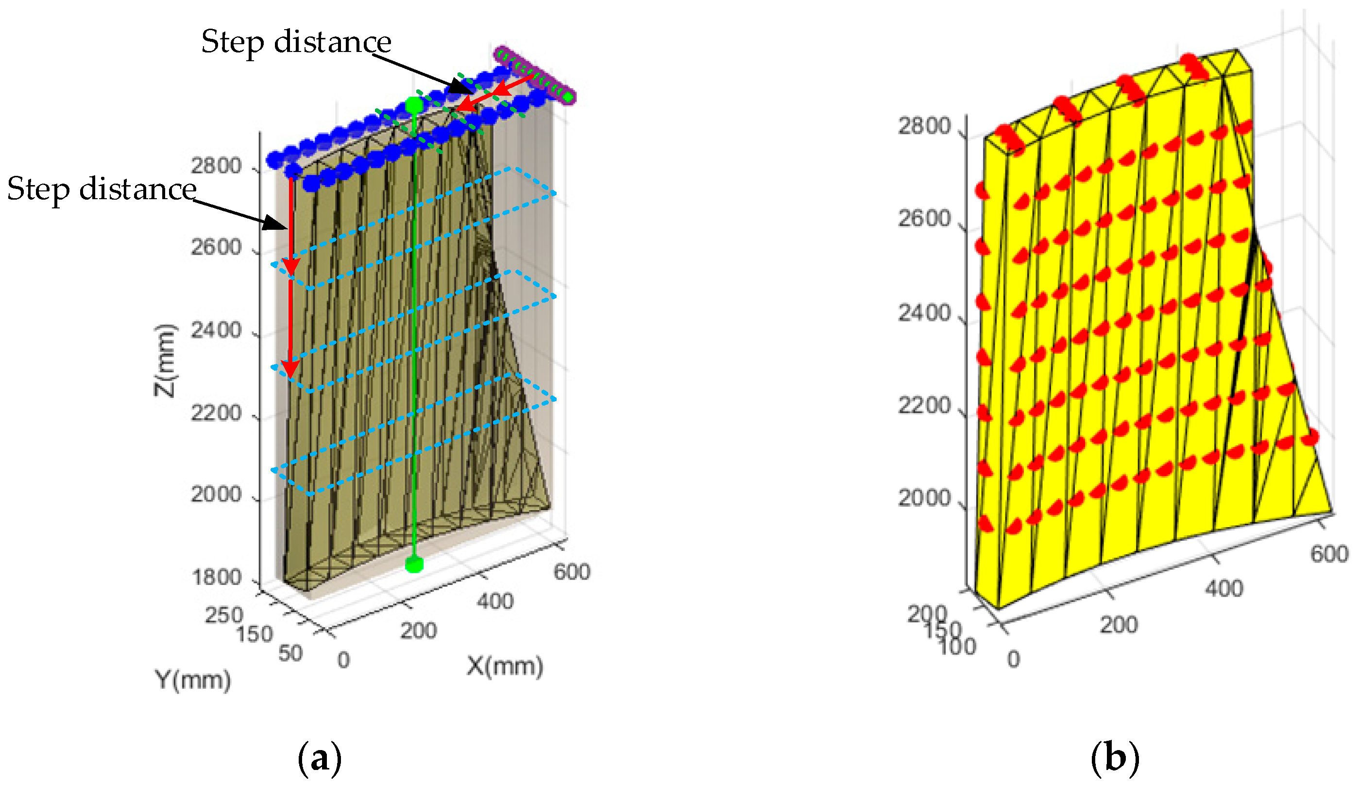
To effectively capture the structural features of the components, discrete points are placed at intervals of 20 mm (configurable), with a step distance of 120 mm (also configurable). Each side of the parallel discrete sampling frame intersects with the outer surface of the component, as illustrated in Figure 11a, resulting in five distinct surface intersections, as shown in Figure 11b. These intersections yield discrete point sets that accurately represent the geometric characteristics of the component’s surface. The selected 20 mm point spacing and 120 mm step length do not directly determine the coordinates of the discrete points but serve to control the density of the linear sampling frame and the layer spacing in the scanning sequence. The actual discrete points are dynamically calculated based on line–triangle intersection algorithms. This parameter combination was configured under a scanning distance of approximately 30 cm and a field of view of 275 mm × 250 mm, taking into account the surface curvature reconstruction accuracy, path redundancy, and scanning efficiency. These values are adjustable and can be flexibly set according to the scanner’s viewing window and the desired modeling quality. Preliminary tests on typical aerospace surface models have shown good stability and repeatability. Further systematic evaluation is in progress and will be presented in future publications.

A linear object can be expressed as a ray or a straight line in a parametric formula, as shown in Formula (14).

$$L\left(t\right)=O+tD,t\in R$$

(14)

in which

$L\left(t\right)$ denotes the point of a linear object (ray or line);

$O$ is the starting point of the ray (or a point on the straight line);

$D$ is the direction vector of the line;

$t$ is a parameter variable that determines the position of the point on the line.

The mathematical representation of a triangular plane is that a triangular aircraft is defined by three $V_0,V_1,V_2$ vertices, which together represent a triangle. The plane’s plane formula can be obtained using cross and dot products. First, two edge vectors are calculated:

$$e_1=V_1-V_0$$

(15)

$$e_2=V_2-V_0$$

(16)

The normal vector $N$ of the plane is the cross product of these two edge vectors.

$$N=e_1\cdot e_2$$

(17)

The formula for the plane of the triangular surface is

$$N\cdot \left(P-V_0\right)=0$$

(18)

$P$ is an arbitrary point on the plane.

To determine whether the linear object intersects with the triangular patch, it is first necessary to check whether the line intersects with the plane where the patch is located. Substituting the parameter formula of the linear object into the formula of the aircraft, the parameter $t$ of the intersection point can be obtained.

The condition for the intersection of the linear object $L\left(t\right)$ and the triangular plane is to substitute the linear formula into the plane formula:

$$N\cdot \left(O+tD-V_0\right)=0$$

(19)

The parameter $t$ can be obtained by solving this formula:

$$t={\displaystyle \frac{N\cdot \left(V_0-O\right)}{N\cdot D}}$$

(20)

If the denominator is $N\cdot D=0$, then the line is parallel to or in the plane of the triangle.

After judging whether the intersection point is solved in the triangular plane to obtain $t$, it is substituted into the linear formula to calculate the intersection point $P=O+tD$. Now, it is necessary to determine whether this point $P$ is located inside the triangle. The barycentric coordinate method can be used to determine

$$P=V_0+\mu \left(V_1-V_0\right)+\nu \left(V_2-V_0\right)$$

(21)

where $\mu$ and $\nu$ are parameters that satisfy

$$\mu \ge 0,\nu \ge 0,\mu +\nu \le 1$$

(22)

By solving this system of formulas, if we find that $\mu$ and $\nu$ satisfy the above conditions, the intersection point is in the triangle.

3.3. Obtaining the Normal Vector of the Intersection Point

Each intersection point corresponds to a specific triangular surface patch, and its associated normal vector reflects the local orientation and spatial direction of the surface at that location. In three-dimensional space, the normal vector is a critical parameter for characterizing the surface topography and plays a vital role in scanning path construction. It provides essential guidance for subsequent path planning and scanner pose adjustments.

During the scanning task, the robot operates by translating its motion so that the pose of the tool center point (TCP) aligns point by point with the pose of each predefined scanning path point until the entire trajectory is completed. Therefore, accurately defining the spatial orientation of each point along the scanning path is essential for achieving high-quality data acquisition. To this end, the normal vector of the triangular surface patch associated with each intersection point can be extracted to represent the local orientation of the path point. By combining this normal information with the acquisition characteristics of the scanning device, a new path point can be generated along the normal direction. This method ensures an ideal angle between the laser beam and the surface normal during scanning, thereby significantly improving both the accuracy of the scan and the completeness of the resulting point cloud data.

These path points represent key positions in the scanning process, ensuring that the scanning device effectively covers the entire surface of the model. Based on the base coordinate system, the coordinates of the points, augmented with their corresponding normal directions, are output. A subset of the path point coordinates and their associated roll–pitch–yaw (RPY) angles is presented in

Table 2. Partial intersection point coordinates.

Name	X	Y	Z	θx	θy	θz
point 1	42.28	100.15	2734.52	79.83	169.60	92.14
point 3	84.55	107.56	2734.52	83.13	172.79	92.17
point 4	126.83	112.65	2734.52	83.13	172.79	92.17
point 5	169.11	116.68	2734.52	86.43	175.81	92.19
point 6	211.38	119.32	2734.52	86.43	175.81	92.19
point 7	253.66	120.04	2734.52	89.73	177.78	92.20
point 8	295.94	119.90	2734.52	93.02	176.25	92.21
point 9	338.21	117.66	2734.52	93.02	176.25	92.21
point 10	380.49	114.21	2734.52	96.32	173.30	92.21
point 11	422.76	109.52	2734.52	96.32	173.30	92.21
point 12	465.04	102.92	2734.52	99.39	170.36	92.20

. Its format is $\left\{x,y,z,{\theta }_x,{\theta }_y,{\theta }_z\right\}$.

3.4. Trajectory Calculation and Output

In planning the scanning path across the five surfaces, the objective is to visit each point exactly once, starting from any point in the given set, and to determine the shortest possible path that connects all points. To achieve efficient path planning, this study employs the nearest neighbor algorithm. At each step, the algorithm selects the closest unvisited point to the current point, progressively constructing a complete traversal path. This method is well suited to scenarios involving a large number of points and high computational complexity. The total length of the resulting path is defined as

$$\min F={\displaystyle \sum _{i=1}^{n-1}{l}_i}$$

(23)

where $F$ is the total length of the path, and $n$ is the number of path points.

The shortest scanning path planning process for components is shown in Figure 12. The specific algorithm idea is as follows: (1) Put the space of scanning path points of components into a set as $C$, and then find an empty set $S$; (2) secondly, a point $Q_1$ is taken from the set $C$ as the starting point and put into the set $S$, and then the nearest neighbor is selected from the set $C$; that is, the closest point to the current distance $Q_1$ is recorded as $Q_2$, and $Q_2$ is taken out and put into the set $S$. At the same time, $Q_2$ is updated as the initial point, and the nearest point to $Q_2$ searched from the set $C$ is recorded as $Q_3$. (3) Continue to repeat step 2 until all of the spatial scanning path points in the set $C$ have been taken out; the spatial scanning path points in the set $S$ are connected in order, and the connection order is the shortest scanning path for the component scanning measurements.

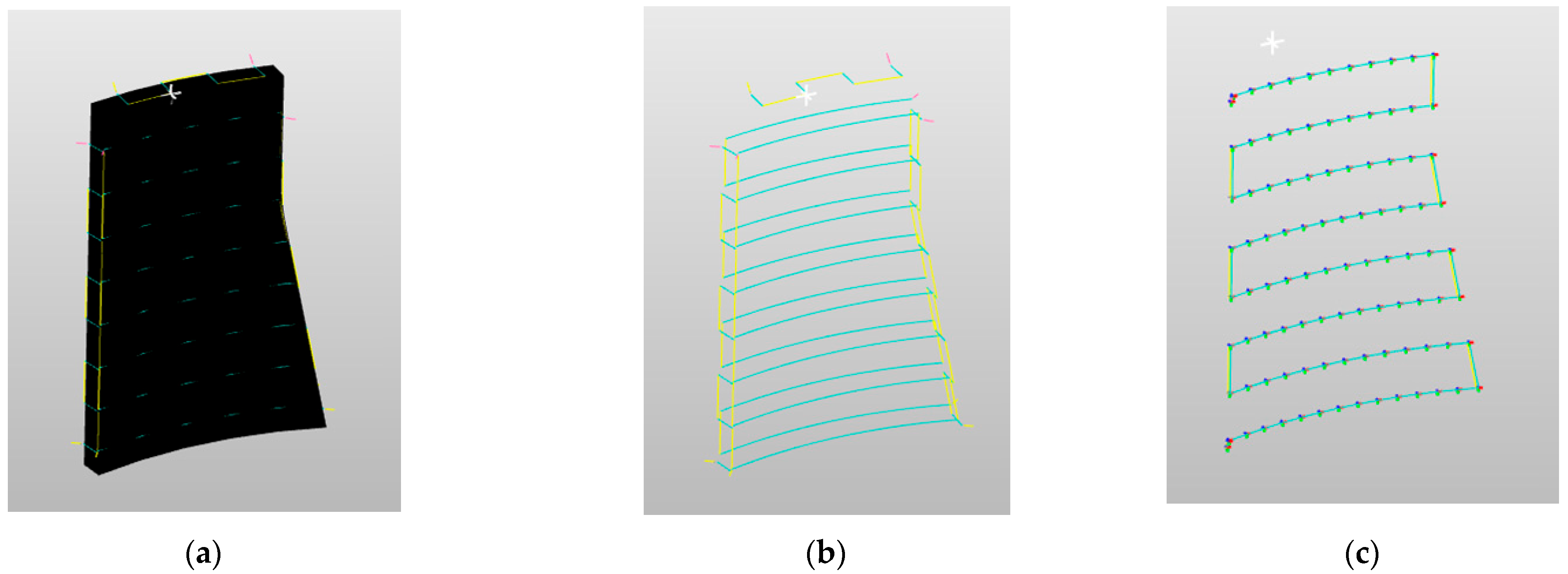
To ensure smooth transitions between scanning path points, this study proposes a method that integrates the nearest neighbor algorithm with B-spline interpolation. The nearest neighbor algorithm is first employed to sort the path points by iteratively selecting the closest unvisited point from the current location, starting from an initial reference point. This approach generates an optimized traversal sequence, significantly reducing the total path length and minimizing redundant motion during the robot’s scanning process.

Based on the path sequence generated by the nearest neighbor algorithm, B-spline interpolation is employed to smoothly connect the discrete path points into a continuous scanning trajectory. B-spline interpolation offers excellent smoothness and controllability, allowing the resulting path to avoid sharp angular transitions and enabling natural curvature transitions between segments. Furthermore, the stability of both the curve and the robot’s motion is enhanced by minimizing an objective function related to variation in the path curvature.

Figure 13a–c illustrate the scanning path generated for component measurements using the proposed algorithm.

The target model is decomposed into five bounding surfaces according to the scanning area. The set of discrete path points extracted from the surface is denoted as $P=\left\{P_1,P_2,\dots ,P_n\right\}$, and each point $P_i$ contains the three-dimensional coordinate $\left(x_i,y_i,z_i\right)$. The goal of the nearest neighbor algorithm is to select the unvisited points closest to the current point from the starting point $P_1$ until all points have been traversed. Finally, an optimized path order $P^{\prime }=\left\{P_1^{\prime },P_2^{\prime },\dots ,P_n^{\prime }\right\}$ is generated.

The distance formula is

$$d\left(p_i,p_j\right)=\sqrt{{\left(x_i-x_j\right)}^2+{\left(y_i-y_j\right)}^2+{\left(z_i-z_j\right)}^2}$$

(24)

The nearest neighbor selection rule is

$${P_{k+1}}^{\prime }=\arg \underset{P_j\in P/P^{\prime }}{\min }d\left(P_k^{\prime },P_j\right)$$

(25)

$P_k^{\prime }$ is the current point, and $P/P^{\prime }$ is the set of unvisited points.

Based on the sequence of path points obtained through nearest neighbor sorting, a smooth curve is generated based on B-spline interpolation. Given the path point sequence $P^{\prime }=\left\{P_1^{\prime },P_2^{\prime },\dots ,P_n^{\prime }\right\}$, the control point is $C=\left(C_0,C_1,\dots ,C_m\right)$, and the interpolation curve is expressed as

$$S\left(t\right)={\displaystyle \sum _{i=1}^m{N}_i,k\left(t\right)C_i, t\in \left[t_k,t_{k+1}\right]}$$

(26)

$N_i,k\left(t\right)$ is the B-spline basis function of the $i$-th control point, which is defined as

$$N_i,k\left(t\right)=\left\{\begin{array}{l}1 t_i\le t\le t_{i+1}\\ 0 otherwise\end{array}\right.$$

(27)

For $k>0$,

$$N_i,k\left(t\right)={\displaystyle \frac{t-t_i}{t_{i+k}-t_i}}{N}_i, k-1\left(t\right)+{\displaystyle \frac{t_{i+k+1}-t}{t_{i+k+1}-t_{i+1}}}{N}_{i+1}, k-1\left(t\right)$$

(28)

The generated B-spline curve $S(t)$ is a piecewise polynomial with $C^k$ smoothness (continuous to the k-th derivative).

The objective function of smooth path optimization is

$$\min {\displaystyle \int \begin{array}{c}{t}_m\\ t_0\end{array}}{‖{\displaystyle \frac{d^{2}S\left(t\right)}{d{t}^2}}‖}^{2}dt$$

(29)

The objective function’s physical meaning minimizes the change in the path’s curvature and ensures the motion’s stability.

4. Scanning Robot Trajectory Measurement Simulation

To validate the effectiveness of the proposed scanning path planning strategy, a virtual scanning trajectory was simulated using robot simulation software, ensuring compliance with the three-dimensional scanner’s parameter constraints. The simulation was conducted on the RobotStudio 6.08 platform, where the scanning measurement process was replicated under the planned path conditions. The simulation environment was configured by importing the industrial robot, the aircraft web model, and the scanning head. Tool and base coordinate systems were established on the scanning head, which was mounted onto the robot’s end effector. The position and orientation of the workpiece model were adjusted to ensure it was located within the robot’s effective workspace. In digital measurement systems, the establishment and unification of coordinate systems form the foundation for both measurement accuracy control and motion planning. The robot scanning system depends on coordinate transformation relationships for effective data communication and trajectory execution. The coordinate system configuration used in the simulation is illustrated in Figure 14.

The robot scanning system incorporates several key coordinate systems, including the robot root coordinate system, the base coordinate system, the tool coordinate system, the workpiece coordinate system, and the measurement coordinate system. The root coordinate system is the robot’s intrinsic reference frame, typically defined at the center of the robot base, and serves as the origin for all robot motions. The base coordinate system is a fixed global reference frame, often coinciding with the root coordinate system. It is used to uniformly define the spatial relationship between the robot and the workpiece. The workpiece coordinate system is established on the measured object and describes its geometric position in space. The measurement coordinate system is defined at the center of the optical tracker probe and serves as the reference frame for the 3D scanning process. To facilitate data exchange and motion control across these frames, transformation matrices must be established between each coordinate system and the measurement coordinate system to ensure consistency in spatial referencing. Finally, the tool coordinate system is attached to the robot’s end effector (i.e., the scanning head) and describes the tool’s position and orientation. It serves as the basis for the robot to acquire and control the pose along the scanning trajectory.

The essence of robotic scanning lies in aligning the orientation of the tool’s center point with the surface normal direction of each point on the workpiece. To maintain an optimal scanning distance of 30 cm between the MetraSCAN 3D scanning head and the surface, the position of the tool’s center point must be redefined. In this study, the tool coordinate system is positioned 30 cm along the positive Z-axis of the scanner’s coordinate system, extending from the laser beam aperture of the MetraSCAN 3D head. This definition, based on the structural characteristics of the scanner, ensures that the scanning head consistently operates within the ideal distance and orientation range. The spatial configuration is illustrated in Figure 15.

The scanning parameters are composed of origin coordinates and Euler angles, and the format is $\{x,y,z,\alpha ,\beta ,\gamma \}$. The expressions of the base coordinate system and the tool coordinate system are shown in the formula.

$$P_{base}=\left[\begin{array}{c}{X}_b\\ Y_b\\ Z_b\end{array}\right], RPY=\left({\alpha }_b,{\beta }_b,{\gamma }_b\right)$$

(30)

$$P_{tool}=\left[\begin{array}{c}{X}_t\\ Y_t\\ Z_t\end{array}\right], RPY=\left({\alpha }_t,{\beta }_t,{\gamma }_t\right)$$

(31)

In three-dimensional space, the spatial geometric relationship between the tool coordinate system and the base coordinate system must be clearly defined to enable scanning path generation and coordinate mapping. This relationship is described through pose transformation, which includes both translational and rotational components.

Suppose that the position of the origin of the tool coordinate system in the base coordinate system is

$$t=\left[\begin{array}{c}x\\ y\\ z\end{array}\right]$$

(32)

The Euler angle $\left(\alpha ,\beta ,\gamma \right)$ adopts the $Z-Y-X$ order (that is, first rotate $\gamma$ around the $Z$ axis, then rotate $\beta$ around the $Y$ axis, and finally rotate $\alpha$ around the $X$ axis). Its corresponding rotation matrix $R\left(\alpha ,\beta ,\gamma \right)$ is expressed as

$$R\left(\alpha ,\beta ,\gamma \right)=R_z\left(\gamma \right)\cdot R_y\left(\beta \right)\cdot R_x\left(\alpha \right)$$

(33)

The specific rotation matrix is

$$R_x\left(\alpha \right)=\left(\begin{array}{ccc}1& 0& 0\\ 0& \cos \alpha & -\sin \alpha \\ 0& \sin \alpha & \cos \alpha \end{array}\right)$$

(34)

$$R_y\left(\beta \right)=\left(\begin{array}{ccc}\cos \beta & 0& \sin \beta \\ 0& 1& 0\\ -\sin \beta & 0& \cos \beta \end{array}\right)$$

(35)

$$R_z\left(\gamma \right)=\left(\begin{array}{ccc}\cos \gamma & -\sin \gamma & 0\\ \sin \gamma & \cos \gamma & 0\\ 0& 0& 1\end{array}\right)$$

(36)

Combining the rotation matrix with the translation vector, a homogeneous transformation matrix $T_{tool}^{base}$ from the base coordinate system to the tool coordinate system can be constructed.

$$T_{tool}^{base}=\left[\begin{array}{l}R\left(\alpha , \beta , \gamma \right) t\\ 0 0 0 1\end{array}\right]$$

(37)

$R$ is a 3 × 3 rotation matrix, which represents the rotation of the attitude. $t$ is a translation vector of 3 × 1, which means the translation of the position. The matrix can realize the transformation of the coordinate points. Let the homogeneous coordinates of a point in space in the base coordinate system be

$$P_{base}=\left[\begin{array}{c}{X}_b\\ Y_b\\ Z_b\\ 1\end{array}\right]$$

(38)

Then, the point is represented in the tool coordinate system as follows:

$$P_{tool}={\left(T_{tool}^{base}\right)}^{-1}\cdot P_{base}$$

(39)

Conversely, if the point is in the tool coordinate system, its representation in the base coordinate system is $P_{tool}$:

$$P_{base}=T_{tool}^{base}\cdot P_{tool}$$

(40)

Based on the above transformation formula, the robot’s scanning motion parameters can be derived relative to the tool coordinate system. Notably, no subsequent point exists for interpolation of the final control point of each trajectory segment. Upon completing the calculations, the scanning parameters corresponding to each surface feature are output.

In the workpiece coordinate system, the scanning motion parameters are configured with a simulation speed of $v=0.04 \mathrm{m}/\mathrm{s}$, an acceleration of $a=0.5 {\mathrm{m}/\mathrm{s}}^2$, and an attitude adjustment time limited to 0.5 s. This parameter combination was selected by considering the motion stability of the industrial robot and the dynamic acquisition performance of the MetraSCAN 3D scanner. It was intended to prevent issues such as image vibration, point cloud misalignment, or discontinuities during the scanning process. Once the scanning path program is executed, the robot manipulates the scanner along the planned trajectory. The scanning direction is indicated by yellow arrows, and the path is visualized in blue-green, as shown in Figure 16.

During the simulation of the scanning motion, no interference or collision was observed between the robot, the 3D scanner, and the component. The scanning range fully conformed to the spatial constraints of the scanner, and the execution time closely matched the theoretical analysis, indicating compliance with the robot’s operational requirements and confirming its ability to complete the measurement task. This study successfully implemented offline scanning trajectory planning based on the geometric characteristics of the measured part, and the feasibility of the proposed scanning path planning strategy was effectively verified.

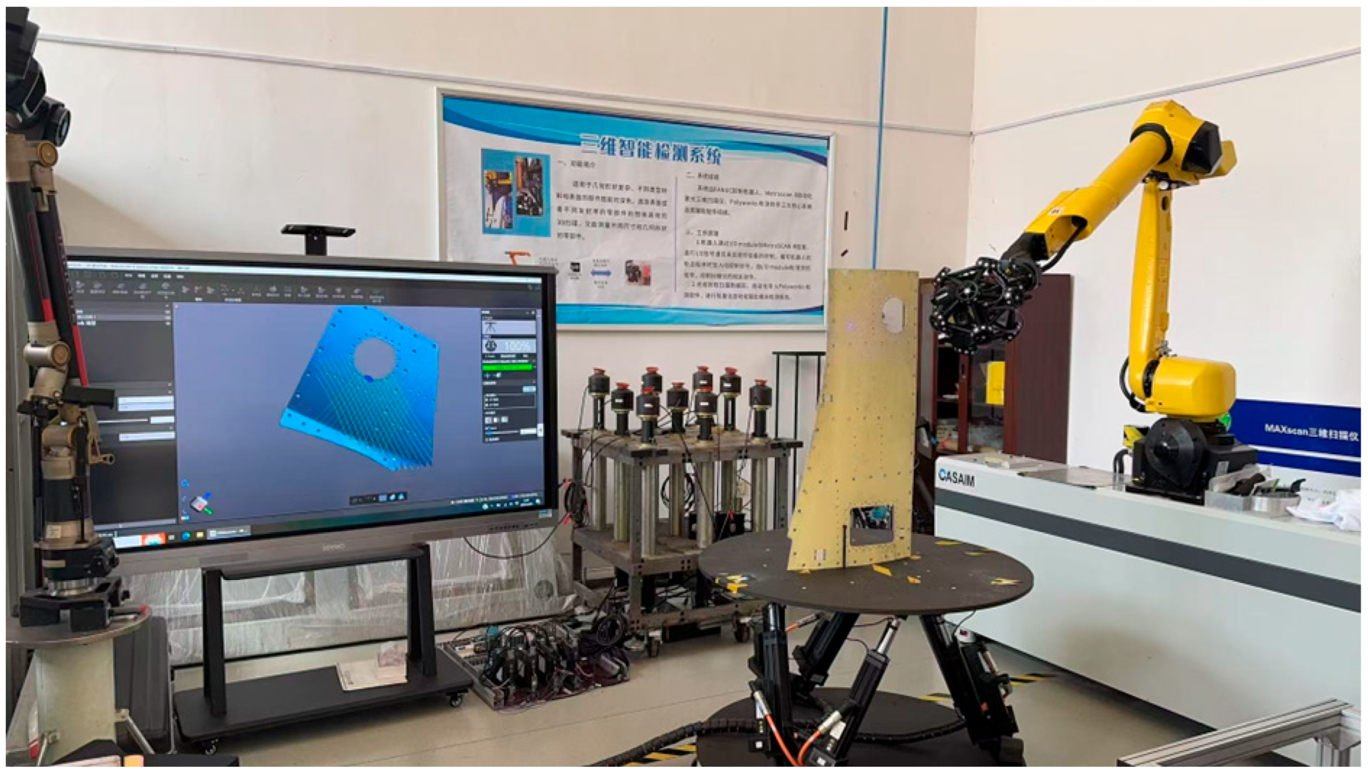
5. The Scanning Measurement Process Experiment

To systematically verify the feasibility of the three-dimensional scanning path planning method proposed in this study for measuring complex components, a scanning reconstruction experiment was conducted using an automated non-contact measurement system. The system integrates an industrial robot, a 3D laser scanning unit, control simulation software, and a data processing platform. The verification experiment was performed based on the scanning trajectory program generated through offline programming in the simulation environment. The experimental setup and procedure are illustrated in Figure 17.

(1)

Experimental system composition

The Industrial Robot: The robot is equipped with an 8 kg payload capacity and a working range of 2032 mm. It features stable trajectory tracking and an excellent dynamic response, enabling precise scanning motion execution. Its control cabinet is integrated with a high-performance motion control interface and an I/O bus system, which supports seamless integration with external laser scanning equipment and upper-level control platforms.

Scanning Equipment: The MetraSCAN 3D laser scanner, developed by Creaform, is capable of high-precision scanning of reflective metallic surfaces, with an array-level accuracy of up to 0.02 mm. In conjunction with VXelements (12) control software, the system enables real-time synchronized acquisition and fusion of both the scanning head’s spatial pose and the corresponding point cloud data, thereby ensuring measurement integrity and spatial accuracy.

(2)

Experimentation

Coordinate System Calibration: Before executing the scanning task, tool center point (TCP) calibration and scanning orientation configuration must be completed. A spatial transformation matrix between the scanner and the robot flange coordinate system is established using a four-point calibration method, thereby enabling a unified control reference system between the two. Additionally, both the laser tracker and the scanner undergo pre-scanning calibration to ensure overall spatial consistency and to maintain the accuracy of the measurement system.

Workpiece Fixation and Experimental Environment Control: The measured workpiece is a representative aviation component featuring a complex, curved surface geometry. To ensure measurement stability, the workpiece is securely mounted onto the platform using a custom-designed positioning fixture, and its position remains unchanged throughout the scanning process. The laboratory environment is maintained at a constant temperature of 23 ± 1 °C, with the relative humidity controlled within the range of 45–55%, to minimize the effects of thermal expansion and fluctuations in the air’s refractive index on laser-based measurements. These environmental controls enhance the repeatability and reliability of the experimental results.

Scanning Acquisition Parameter Configuration: Key scanning parameters, including the shutter speed, resolution, and boundary optimization settings, are preset in the VXelements software to mitigate the impact of noise and isolated points on the point cloud accuracy. A dynamic tracking threshold is defined to prevent occlusion and pose instability during scanning. Additionally, path accessibility and boundary conditions are verified through a manual teaching procedure to ensure the continuity and completeness of the scanning process.

System Stability Verification and Pre-Test Operation: A platform linkage test was conducted prior to the experiment to verify the system’s stability. The test included checks for continuity in robot pose transitions, the integrity of scanner perspective switching, and real-time synchronization of data acquisition. The pose accuracy of the scanner was indirectly validated using a binocular optical tracking system, ensuring that both the robot’s trajectory error and the scanning attitude error remained within acceptable limits. The test results confirmed that the system operated stably and was suitable for subsequent automated scanning experiments involving complex surface geometries.

(3)

Experimental results

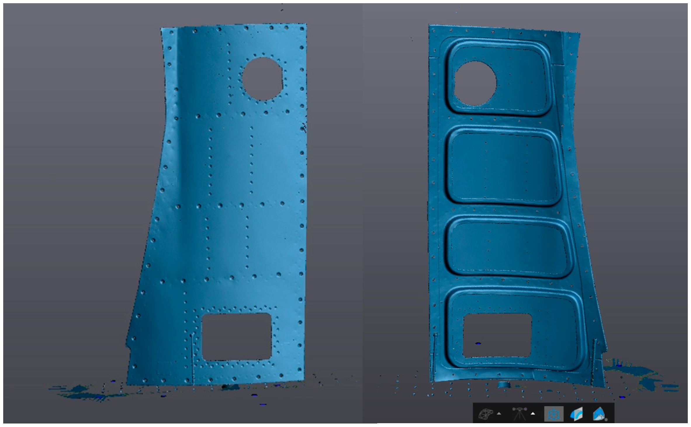
Based on offline programming, the scanning trajectory was automatically generated, and a point cloud model of the aircraft web was reconstructed using the automated scanning system, as illustrated in Figure 18. The experimental results indicate that for typical aviation components, the proposed method improves the overall measurement efficiency by 25.4%, reducing the total measurement time to 8 min. Notably, the scanning execution itself takes only 3 min, representing a substantial improvement compared to the traditional manual method, which requires approximately 10 min. The reconstructed model demonstrates a complete surface topography, continuous point cloud coverage, and no observable noise or missing data, validating the system’s surface reconstruction accuracy and scanning stability for complex geometries. In the performance evaluation of path planning, the method achieved an 18.6% increase in point cloud coverage, with no frame loss or occlusion failures during the scanning process. This reflects a strong multi-axis collaborative control capability and robust pose tracking. Furthermore, the scanning workflow exhibits a high degree of automation and modularization, with effective human–machine interaction and flexible system deployment.

The performance metrics reported in this study were obtained from a comparative experiment using an aircraft floor panel as the target object. The reference method involves manual coordinate point marking and scanning, which is commonly used in industrial practice. Under identical path planning and pose adjustment conditions, we evaluated both approaches in terms of the total measurement time, point cloud completeness, and scanning stability. The manual method requires multiple operator-defined poses and is prone to inefficiencies such as redundant scans, pose discontinuities, and missed areas [21]. In contrast, the proposed automatic path planning system achieves continuous pose transitions and efficient multi-axis coordination without human intervention. All of the data represent the average of three repeated experiments conducted under identical conditions.

In summary, the system demonstrates significant advantages in its measurement accuracy, execution efficiency, and process controllability. It offers a practical solution for non-contact, automated, and high-precision measurement of complex structural components in high-end manufacturing fields such as aerospace. It holds strong potential for engineering applications and intelligent manufacturing integration.

6. Conclusions

To address the challenges of low path planning efficiency and insufficient point cloud coverage in the three-dimensional scanning of significant, structurally complex components, this study proposes an offline scanning path generation and optimization method based on CAD models. The technique is integrated into a non-contact, automated 3D scanning measurement system. The primary research outcomes are summarized as follows:

(1)

An efficient model discretization method is established: An efficient discretization approach is proposed by constructing an optimal oriented bounding box (OBB) and employing a linear object–triangular patch intersection algorithm. This method enables accurate discrete sampling of complex surface geometries and generates a representative point set of the model’s surface, thereby ensuring high-quality input data for subsequent path generation.

(2)

A pose solution model based on surface normals and kinematic constraints: A multi-degree-of-freedom pose solution model is proposed by integrating the normal vector information for discrete surface points with the kinematic constraints of the scanning system. This model enables accurate estimation of the scanner’s spatial orientation and significantly enhances both the enforceability and spatial coverage of the generated scanning path.

(3)

An optimal path generation and interpolation optimization mechanism: An optimal path generation mechanism is developed by introducing an improved nearest neighbor search algorithm to construct a globally optimized scanning trajectory. To enhance the continuity and smoothness, the initial path is refined further using an adaptive B-spline interpolation algorithm. This combined approach effectively minimizes abrupt path changes and redundant robot movements.

(4)

The development of a MATLAB (R2023b) –RobotStudio (6.08) co-simulation platform: A complete closed-loop co-simulation platform is established, integrating CAD model import, discrete sampling, path planning, and virtual simulation. This system enables automatic scanning path generation and online verification, significantly reducing the debugging cycle of the scanning workflow. The effectiveness of the proposed method is verified through experimental evaluation. The results show that compared with the traditional manual teaching method, the proposed approach improves the scanning efficiency by 25.4% and increases the point cloud coverage by 18.6% in three-dimensional measurements of representative structural components, demonstrating substantial practical value and strong potential for engineering application and promotion.

In this study, a representative aircraft belly panel was selected as the validation object due to its complex surface geometry and high-precision requirements, making it a typical and challenging example. However, the proposed method is not limited to such components and can be extended to 3D scanning tasks for complex structural parts in other fields such as automotives, energy, and shipbuilding. The scanning path planning method developed in this work is based on visible geometric features of the outer contour and is primarily applicable to external or semi-open surface regions. For complex internal structures with severe occlusion or a limited line of sight, where laser beams cannot effectively reach the target surface, the method can be extended through structural reconstruction strategies or by employing multi-angle and multi-path rescanning mechanisms. These aspects will be explored further in future studies.