Backstepping-Based Finite-Horizon Optimization for Pitching Attitude Control of Aircraft

Abstract

In this paper, the problem of pitching attitude finite-horizon optimization for aircraft is posed with system uncertainties, external disturbances, and input constraints. First, a neural network (NN) and a nonlinear disturbance observer (NDO) are employed to estimate the value of system uncertainties and external disturbances. Taking input constraints into account, an auxiliary system is designed to compensate for the constrained input. Subsequently, the backstepping control containing NN and NDO is used to ensure the stability of systems and suppress the adverse effects caused by the system uncertainties and external disturbances. In order to avoid the derivation operation in the process of backstepping, a dynamic surface control (DSC) technique is utilized. Simultaneously, the estimations of the NN and NDO are applied to derive the backstepping control law. For the purpose of achieving finite-horizon optimization for pitching attitude control, an adaptive method termed adaptive dynamic programming (ADP) with a single NN-termed critic is applied to obtain the optimal control. Time-varying feature functions are applied to construct the critic NN in order to approximate the value function in the Hamilton–Jacobi–Bellman (HJB) equation. Furthermore, a supplementary term is added to the weight update law to minimize the terminal constraint. Lyapunov stability theory is used to prove that the signals in the control system are uniformly ultimately bounded (UUB). Finally, simulation results illustrate the effectiveness of the proposed finite-horizon optimal attitude control method.

1. Introduction

In flight control, the problem of finite-horizon optimization for pitching attitude tracking control of aircraft can be treated as the pitching attitude tracking the command signal with the desired finite-horizon optimal index. To resolve the above problem, both the tracking control and finite-horizon optimization should be taken into consideration, which makes the overall problem significantly difficult.

In order to achieve attitude tracking for aircraft, much research has been conducted. In [1], an adaptive second order sliding model control method was presented in order to improve the performance in the presence of external disturbances. In [2], a gain-scheduling control method was proposed for linear parameter-varying systems with multi-input multi-output in order to obtain a satisfactory performance in the bank-to-turn control of aircraft. In [3], nonlinear dynamic inversion technology was proposed for the design of a supermaneuverable aircraft control. In [4], backstepping control was employed to execute the attitude tracking control of a mini unmanned aerial vehicle.

Among the control methods above, the backstepping control scheme is widely used owing to some advantages. First, virtual control is designed separately for each subsystem in the process of backstepping control to reduce the complexity of high-order system control. Subsequently, the backstepping control can be combined with other control methods such as sliding mode control, NN, adaptive control method, and disturbance observer to improve the control performance. In [5], a robust backstepping control scheme combining sliding mode control and neural network (NN) was proposed to achieve the reentry attitude tracking control of a near-space hypersonic vehicle in the presence of parameter variations and external disturbances. In [6], a deep convolutional NN-based backstepping method was used to identify system uncertainties and hidden states in attitude control in order to enhance the robustness. In [7], an auxiliary system-based backstepping control was constructed for the aircraft subject to the input saturation problem caused by wing rock. In [8], a finite-time convergence backstepping control scheme was designed. In the scheme, a finite-time observer and finite-time auxiliary system were used to suppress the effects of unsteady aerodynamic disturbances and compensate for the effect of input saturation, respectively. However, the aforementioned attitude control methods do not take into account the optimal control that meets some desired index. Actually, the optimal control problem is intractable, especially for a nonlinear system. Hence, there is relatively little research on the attitude control of aircraft in an optimal way, which is a nonlinear optimization problem in nature, not to mention the finite-horizon optimization for attitude tracking control. Thus, how to control the aircraft attitude in an optimal way should be further studied.

Quadratic optimal control is an optimal control method applied earlier in flight control. A given quadratic index is used to control the system with a desired optimal performance. In [9], a nonlinear system was divided into two parts of a linear nominal system and compound disturbances. Then, a linear quadratic regulator was designed to control the linear nominal system, while a robust control was derived to compensate for the effects caused by compound disturbances. In order to cope with the problem of recovering open-loop singular values in the quadratic optimal control, the LQG/LTR technique was applied for a multivariable vertical short take-off and landing aircraft linear system in [10]. However, the above control methods can only be applied to linear systems. For a nonlinear system, Hamilton–Jacobi–Bellman (HJB) equations without analytical solutions need to be solved, which makes it intractable to execute optimal control.

To cope with the problem of solving HJB equations for a nonlinear system, some numerical methods were applied to approximate the solution. In [11], a dynamic programming algorithm was presented, which is supposed to be solved in an off-line manner. In [12], a recursive optimization approach was proposed for a nonlinear system. In [13], a state-dependent Riccati equation (SDRE) method, which used a parameterization technique to convert the nonlinear system into a linear structure with state-dependent coefficients, was proposed to deal with the problem of nonlinear optimization. Nevertheless, a heavy computational burden is the main obstacle to applying the above three methods to nonlinear optimization. Inspired by the dynamic programming algorithm, the ADP algorithm was proposed in [14]. Compared with the dynamic programming algorithm, a critic NN was constructed to approximate the value function in order to solve the HJB equation forward-in-time in the ADP algorithm. Thus, the heavy computational burden was avoided, and on-line optimization was achieved.

The ADP algorithm, characterized by strong abilities of self-learning and adaptivity, has received significantly increased attention and has become an important intelligent optimal control method for nonlinear systems [15]. Due to its advantage of a low calculation cost, ADP has been applied in flight control. In [16], an adaptive critic design (ACD)-based optimal control algorithm was proposed. Under the premise of ensuring system stability, the ACD algorithm was utilized to improve the control performance of the system. In [17], a constrained ADP approach and linear parameter-varying technique were employed to guarantee the closed-loop stability and excellent control performance of the flight with aerodynamic parameter uncertainties and actuator failures. In [18], an incremental ADP algorithm was proposed to control the attitude tracking of spacecraft. In [19], an integral sliding-mode control based adaptive actor–critic algorithm was developed to guarantee the optimal control for sliding-mode dynamics online. As discussed above, the backstepping control method is favored by researchers due to its advantages. Because of its feature of easy combination with other control methods, the backstepping-based ADP scheme has been applied in many works. In [20], a backstepping-based ADP algorithm was developed to solve the problem of missile-target interception with state and input constraints. In the scheme of backstepping, a barrier Lyapunov function was used in the virtual controller design process for each subsystem to guarantee the state constraints, and an auxiliary system was designed to compensate for the constrained input. In [21], a backstepping-based ADP algorithm with zero-sum differential game method was applied to the zero-sum game problem for a missile and target. The zero-sum differential game technique was applied in the scheme of ADP algorithm in order to control the missile and target in an optimal way, and a critic network was constructed to approximate the value function in Hamilton–Jacobi–Isaacs (HJI) in order to achieve optimization online. In [22], an NN-based optimal control scheme was proposed for the near-space vehicle attitude tracking control. In the scheme, the NN and NDO were designed in a backstepping scheme to approximate the system uncertainties and external disturbances, while the critic network was constructed to approximate the value function in the HJB equation. However, it should be noted that the developments of the ADP algorithm above mainly address only the problem of infinite-horizon optimization. In fact, it is required to control in a finite-horizon optimal way for many systems, especially for flight systems.

Compared with infinite-horizon optimal control, finite-horizon optimal control is considered to be more challenging. First, the value function of the finite-horizon optimal control system is time-to-go-dependent, which leads to a time-varying associated HJB equation. Hence, it is more difficult to solve the HJB equation. Second, the terminal constraint should be taken into account for infinite-horizon optimization [23]. For the purpose of addressing the issues above, some research has been conducted. In [24], time-dependent weights and state-dependent feature functions were incorporated to construct an NN in order to approximate the time-to-go-dependent value function, and the least-square-based gradient descent method was utilized to update the weights off-line. In contrast, an NN consisting of constant weights and time-state-dependent feature functions was designed to achieve the approximation of the value function in the HJB function online in [25]. Nevertheless, the constrained input and system uncertainties were not taken into account. Considering input constraints, a non-quadratic function was utilized to eliminate the input constraints in [26]. Regarding system uncertainties, an online NN identifier was designed to approximate system uncertainties, and an actor–critic algorithm was introduced to solve the HJB equation to guarantee that the system was controlled with the optimal index in finite-horizon in [27]. Unfortunately, most of the research considered discrete systems. Furthermore, the constrained input, system uncertainties, and external disturbances are not considered in the finite-horizon optimal control together, which limits its application in flight control.

In order to address the problem of finite-horizon optimization pitching attitude tracking with system uncertainties, external disturbances, and input constraints, a novel backstepping-based finite-horizon optimization is developed in this work. The backstepping scheme, in which NN and NDO are employed to estimate the value of system uncertainties and external disturbances and an auxiliary system is designed to compensate for the constrainted input, is introduced to ensure the stability of systems. The ADP algorithm with a critic NN that consists of constant weights and time-state-dependent feature functions is employed to obtain finite-horizon optimal control. A novel updating law of the critic NN weights is derived to solve the HJB equation and minimize the terminal constraints. Furthermore, the Lyapunov stability method is applied to prove that the signals in the control system are UUB. Finally, simulation results illustrate the effectiveness of the proposed control scheme.

The main contributions of this paper include the following:

(1)

A backstepping-based ADP scheme is used to achieve finite-horizon optimal control. In the backstepping control scheme, NN is applied to approximate system uncertainties, while NDO is employed to estimate external disturbances. The ADP is used to control the nominal system in a finite-horizon optimal manner. Due to the integration of the backstepping method and the advantages of ADP, the backstepping-based finite-horizon optimization ADP scheme is promising for pitching attitude tracking control.

(2)

A novel updating law of the critic NN weights is derived in order to satisfy the terminal constraints, relaxing the requirement of an initial admissible control and guarantee the stability of system.

The rest of the paper is organized as follows. Section 2 formally states the preliminaries of the research object of this paper. The desigsn for backstepping control and finite-horizon optimal control are given in Section 3 and Section 4, respectively. Then, the stability analysis is developed in Section 5. The simulation results are presented in Section 6. Finally, the conclusions of the paper are given in the last section.

Notations. Throughout the paper, $R^{m\times n}$ stands for the set of all $m\times n$ real matrices. ${\nabla }_{x}f$ stands for the gradient of f with respect to x such as ${\nabla }_{x}f={\displaystyle \frac{\partial f}{\partial x}}$. $sign(·)$ stands for the sign function.

2. Problem Descriptions and Preliminaries

Before giving the attitude dynamics of an aircraft, a diagram illustrating the model parameters of the aircraft is given in

Table 1. The illustration of aircraft model parameters.

$\alpha$	angle of attack	$\gamma$	flight path angle
q	pitching rate	$I_{yy}$	moment of inertia
${\delta }_z\left(u\right)$	constrained normal thrust vectoring angle	$\overline{q}$	dynamic pressure
M	mass of aircraft	S	reference surface area of wing
V	airspeed of aircraft	$\overline{c}$	mean aerodynamic chord
L	lift force	$C_m$	pitch moment aerodynamic coefficient
T	thrust	$x_T$	distance between engine nozzle and center of mass

. Regardless of the unsteady aerodynamics, the longitudinal attitude dynamics of an aircraft with system uncertainties and external disturbances can be described as follows [7].

$$\dot{\alpha }=f_1\left(\alpha \right)+q+\Delta f_1\left(\alpha \right)+d_1,$$

(1)

$$\dot{q}=f_2(\alpha ,q)+g_2{\delta }_z\left(u\right)+\Delta f_2(\alpha ,q)+d_2,$$

(2)

where $f_1\left(\alpha \right)\in R^1$ and $f_2(\alpha ,q)\in R^1$ are the known internal system dynamics. $g_2\in R^1$ is the known control coefficient. $u\in R^1$ is the unconstrainted control to be designed. $\Delta f_1\left(\alpha \right)\in R^1$ and $\Delta f_2(\alpha ,q)\in R^1$ are the unknown system uncertainties. $d_1\in R^1$ and $d_2\in R^1$ are the unknown external disturbances. $f_1\left(\alpha \right)$, $f_2(\alpha ,q)$, $g_2$, ${\delta }_z\left(u\right)$ are given by

$$f_1\left(\alpha \right)={\displaystyle \frac{1}{MV}}(-L-Tsin\alpha +Mgcos\gamma ),$$

(3)

$$f_2(\alpha ,q)={\displaystyle \frac{\overline{q}S\overline{c}{C}_m}{I_{yy}}},$$

(4)

$$g_2={\displaystyle \frac{1}{I_{yy}}}{x}_{T}T{\displaystyle \frac{\pi }{180}},$$

(5)

$${\delta }_z=\left\{\begin{array}{c}{u}_{M}sign\left(u\right),\left|u\right|\ge u_M\hfill \\ u,\left|u\right|<u_M\hfill \end{array},\right.$$

(6)

where $u_M$ is a known boundary of u.

In this paper, the control objective is to design a controller u, so that the angle of attack $\alpha$ is driven to track a desired signal ${\alpha }_c$ in a finite-horizon optimal manner, and all the signals in the control system (1) and (2) are uniformly ultimately bounded (UUB). To illustrate the design of the proposed method, the control block diagram is shown in Figure 1. To deal with the external disturbances and the system uncertainties, the NDO and the NN are designed together with the backstepping control. To solve the problem of the input constraints, the auxiliary is used in the forward control, which transforms the longitudinal attitude dynamics of the aircraft into the nominal form. To carry out optimal control, the ADP-based finite-horizon optimal control method is designed with the critic NN.

For the design of the controller hereinafter, the following assumption is required.

Assumption 1. 

In Equations (1) and (2), the system uncertainties $\Delta f_1\left(\alpha \right)$ and $\Delta f_2(\alpha ,q)$ as well as the external disturbances $d_1$ and $d_2$ are differentiable. In addition, the first derivatives of $d_1$ and $d_2$ are bounded such as $\dot{\left|d_1\right|}\le {\dot{d}}_{1M}$. Furthermore, $g_2$ is invertible and bounded such as $0<\left|g_2\right|\le g_{2M}$.

Remark 1. 

Investigating the expression of $g_2$ shown as Equation (5), the boundeness of $I_{yy}$, $x_T$, and T yield the boundness of $g_2$, and the non-zero values of $x_T$ and T make $g_2$ invertible. Thus, Assumption 1 is reasonable.

3. Design for Backstepping Control

In this section, a backstepping method with NN and NDO is derived to design a forward controller. The NN is constructed to approximate the system uncertainties while the NDO is designed to approximate the external disturbances. Then, the system comprising (1) and (2) is transformed into a nominal system to be controlled in a finite-horizon optimal manner by ADP.

In order to obtain satisfying control performance, the negative effects caused by unknown system uncertainties must be eliminated. According to the NN theory, the system uncertainties $\Delta f_1\left(\alpha \right)$ and $\Delta f_2(\alpha ,q)$ can be approximated as [22]

$$\Delta f_1\left(\alpha \right)=L_1^{-1}(W_1^{*T}{a}_1\left(\alpha \right)+r_1^{*}),$$

(7)

$$\Delta f_2(\alpha ,q)=L_2^{-1}(W_2^{*T}{a}_2(\alpha ,q)+r_2^{*}),$$

(8)

where $L_1\in R^1$, $L_2\in R^1$ are the parameters to be designed. $a_1\left(\alpha \right)\in R^{n_1}$ and $a_2(\alpha ,q)\in R^{n_2}$ are basis functions. $n_1$ and $n_2$ are the numbers of the basis functions of $a_1\left(\alpha \right)$ and $a_2(\alpha ,q)$, respectively. $W_1^{*}\in R^{n_1}$ and $W_2^{*}\in R^{n_2}$ are the desired weight vectors. $r_1^{*}$ and $r_2^{*}$ are the approximation errors of the NN.

Assumption 2 

([20]). $W_1^{*}$ and $W_2^{*}$ are both bounded as $∥W_1^{*}∥\le W_{1M}^{*}$, $∥W_2^{*}∥\le W_{2M}^{*}$.

Invoking Equations (7) and (8) into (1) and (2) yields

$$\dot{\alpha }=f_1\left(\alpha \right)+q+L_1^{-1}{W}_1^{*T}{a}_1\left(\alpha \right)+D_1,$$

(9)

$$\dot{q}=f_2(\alpha ,q)+g_2{\delta }_z\left(u\right)+L_2^{-1}{W}_2^{*T}{a}_2(\alpha ,q)+D_2,$$

(10)

where $D_1=L_1^{-1}{r}_1^{*}+d_1\in R^1$ and $D_2=L_2^{-1}{r}_2^{*}+d_2\in R^1$ are treated as compound disturbances [22].

For the purpose of compensating for input constraints, an auxiliary system is designed as

$${\dot{S}}_2=-k_{aux}{S}_2+g_2\Delta ,$$

(11)

where $\Delta ={\delta }_z\left(u\right)-u$. $S_2\in R^1$ is an auxiliary control signal. $k_{aux}$ is the parameter to be designed.

Assumption 3 

([8]). Δ is bounded such as $∥\Delta ∥\le \overline{\Delta }$.

The error system is defined as [20,22]

$$z_1=\alpha -{\alpha }_c,$$

(12)

$$z_2=q-q_c-S_2,$$

(13)

where $q_c\in R^1$ is the virtual control law to be designed.

Invoking Equations (9)–(11), the dynamics of the error system are derived as

$${\dot{z}}_1=f_1\left(\alpha \right)+q+L_1^{-1}{W}_1^{*T}{a}_1\left(\alpha \right)+D_1-{\dot{\alpha }}_c,$$

(14)

$$\begin{array}{c}{\dot{z}}_2=f_2(\alpha ,q)+g_{2}u+L_2^{-1}{W}_2^{*T}{a}_2(\alpha ,q)+D_2-{\dot{q}}_c+k_{aux}{S}_2\hfill \end{array}.$$

(15)

For the purpose of achieving the backstepping control and finite-horizon optimal control, both of the virtual control $q_c$ and the unconstrained control u are divided into two parts as

$$q_c=q_c^a+q_c^{*},$$

(16)

$$u=u^a+u^{*},$$

(17)

where $q_c^a$ and $u^a$ are the virtual control input and unconstrained control input in the backstepping scheme, respectively, and $q_c^{*}$ and $u^{*}$ are the virtual control input and unconstrained control input in the finite-horizon optimal control scheme, respectively.

To estimate the compound disturbances, NDOs are designed as [22]

$$\left\{\begin{array}{c}{\widehat{D}}_1={\varsigma }_1+H_1\left(\alpha \right)\hfill \\ {\dot{\varsigma }}_1=-L_1(f_1\left(\alpha \right)+q+{\widehat{D}}_1)-{\widehat{W}}_1^T{a}_1\left(\alpha \right)+z_1\hfill \end{array},\right.$$

(18)

$$\left\{\begin{array}{c}{\widehat{D}}_2={\varsigma }_2+H_2\left(q\right)\hfill \\ {\dot{\varsigma }}_2=-L_2(f_2(\alpha ,q)+g_2{\delta }_z\left(u\right)+{\widehat{D}}_2)-{\widehat{W}}_2^T{a}_2(\alpha ,q)+z_2\hfill \end{array},\right.$$

(19)

where ${\widehat{D}}_1$ and ${\widehat{D}}_2$ are the estimations of $D_1$ and $D_2$, respectively. $H_1\left(\alpha \right)\in R^1$ and $H_2\left(\alpha \right)\in R^1$ are functions to be designed that satisfy $L_1=\partial H_1\left(\alpha \right)/\phantom{\partial H_1\left(\alpha \right)\partial }\partial \alpha$ and $L_2=\partial H_2\left(q\right)/\phantom{\partial H_2\left(q\right)\partial }\partial q$. ${\widehat{W}}_1$ and ${\widehat{W}}_2$ are the estimations of $W_1^{*}$ and $W_2^{*}$, respectively.

We define the estimation errors as

$${\tilde{W}}_1={\widehat{W}}_1-W_1^{*}$$

(20)

$${\tilde{W}}_2={\widehat{W}}_2-W_2^{*}$$

(21)

$${\tilde{D}}_1=D_1-{\widehat{D}}_1$$

(22)

$${\tilde{D}}_2=D_2-{\widehat{D}}_2.$$

(23)

Invoking Equations (9), (10), (18), (19), (22), and (23), the dynamics of ${\tilde{D}}_1$ and ${\tilde{D}}_2$ can be written as

$${\dot{\tilde{D}}}_1={\dot{D}}_1-L_1{\tilde{D}}_1+{\widehat{W}}_1^T{a}_1\left(\alpha \right)-z_1$$

(24)

$${\dot{\tilde{D}}}_2={\dot{D}}_2-L_2{\tilde{D}}_2+{\tilde{W}}_2^T{a}_2(\alpha ,q)-z_2.$$

(25)

Then, the backstepping control law can be designed as follows.

Step 1: Taking Equation (14) into account, the virtual control input $q_c^a$ is designed as

$$q_c^a=-(k_1{z}_1+f_1\left({\alpha }_c\right)+L_1^{-1}{\widehat{W}}_1^T{a}_1\left(\alpha \right)+{\widehat{D}}_1-{\dot{\alpha }}_c),$$

(26)

where $k_1$ is the parameter to be designed.

The weights vector ${\widehat{W}}_1$ is updated as

$${\dot{\widehat{W}}}_1={\mathrm{\Omega }}_1^{-1}(a_1\left(\alpha \right)z_1^T{L}_1^{-1}-{\tau }_1{\widehat{W}}_1),$$

(27)

where ${\mathrm{\Omega }}_1\in R^{n_1\times n_1}$ is the positive definite symmetric matrice to be designed [22]. ${\tau }_1$ is the parameter to be designed.

Invoking Equations (13), (14), (16), and (26) yields

$$\begin{array}{c}{\dot{z}}_1=f_1\left(\alpha \right)-f_1\left({\alpha }_c\right)+q_c^{*}+z_2-k_1{z}_1-L_1^{-1}{\tilde{W}}_1^T{a}_1\left(\alpha \right)+{\tilde{D}}_1+S_2\hfill \end{array}.$$

(28)

In the normal backstepping scheme, it is inevitable to differentiate $q_c$. Nevertheless, due to the unknown information in the partial derivative of $q_c$, it is intractable to obtain the derivation. In order to avoid the derivation operation, a dynamic surface control (DSC) technique is applied as [28]

$$\tau \dot{\lambda }+\lambda =q_c,\lambda \left(0\right)=q_c\left(0\right),$$

(29)

where τ is the parameter to be designed. λ is a first-order filter in nature to approximate $q_c$ such that $\dot{\lambda }$ can substitute for ${\dot{q}}_c$.

We define the error as

$$e=\lambda -q_c.$$

(30)

Then, we have

$$\begin{array}{c}\dot{e}=\dot{\lambda }+(-{\dot{q}}_c)\hfill \\ =-e/\phantom{-e\tau }\tau +(-{\displaystyle \frac{\partial q_c}{\partial \alpha }}\dot{\alpha }-{\displaystyle \frac{\partial q_c}{\partial {\alpha }_c}}{\dot{\alpha }}_c-{\displaystyle \frac{\partial q_c}{\partial z_1}}{\dot{z}}_1-{\displaystyle \frac{\partial q_c}{\partial {\widehat{W}}_1}}{\dot{\widehat{W}}}_1-{\displaystyle \frac{\partial q_c}{\partial {\widehat{D}}_1}}{\dot{\widehat{D}}}_1-{\displaystyle \frac{\partial q_c}{\partial {\dot{\alpha }}_c}}{\ddot{\alpha }}_c-{\displaystyle \frac{\partial q_c}{\partial {\widehat{W}}_c}}{\dot{\widehat{W}}}_c)\hfill \\ =-e/\phantom{-e\tau }\tau +M_d(z_1,z_2,e,{\widehat{W}}_1,{\widehat{D}}_1,{\widehat{W}}_2,{\alpha }_c,{\dot{\alpha }}_c,{\ddot{\alpha }}_c)\hfill \end{array},$$

(31)

where $M_d(z_1,z_2,e,{\widehat{W}}_1,{\widehat{D}}_1,{\alpha }_c,{\dot{\alpha }}_c,{\ddot{\alpha }}_c)=-{\displaystyle \frac{\partial q_c}{\partial \alpha }}\dot{\alpha }-{\displaystyle \frac{\partial q_c}{\partial {\alpha }_c}}{\dot{\alpha }}_c-{\displaystyle \frac{\partial q_c}{\partial z_1}}{\dot{z}}_1-{\displaystyle \frac{\partial q_c}{\partial {\widehat{W}}_1}}{\dot{\widehat{W}}}_1-{\displaystyle \frac{\partial q_c}{\partial {\widehat{D}}_1}}{\dot{\widehat{D}}}_1-{\displaystyle \frac{\partial q_c}{\partial {\dot{\alpha }}_c}}{\ddot{\alpha }}_c-{\displaystyle \frac{\partial q_c}{\partial {\widehat{W}}_c}}{\dot{\widehat{W}}}_c$. ${\widehat{W}}_c\in R^L$ is the weight vector of critic NN designed hereinafter.

Assumption 4 

([28]). $M(z_1,z_2,e,{\widehat{W}}_1,{\widehat{D}}_1,{\alpha }_c,{\dot{\alpha }}_c,{\ddot{\alpha }}_c)$ is a continuous function. For any $C_1$ and $C_2$, the sets ${\Pi }_1:=\{({\alpha }_c,{\dot{\alpha }}_c,{\ddot{\alpha }}_c):{\alpha }_c^2+{\dot{\alpha }}_c^2+{\ddot{\alpha }}_c^2\le C_1\}$ and ${\Pi }_2:=\{{\sum }_{j=1}^2{z}_j^2+{\tilde{W}}_1^T{\mathrm{\Omega }}_1{\tilde{W}}_1+{\tilde{W}}_c^T{\tilde{W}}_c+e^2+{\tilde{D}}_1^2+{\ddot{\alpha }}_c^2\le C_2\}$ are compact in $R^3$ and $R^{5+n_1+L}$, respectively. Hence, ${\Pi }_1\times {\Pi }_2$ is also compact. Considering the continuous property, the function $M_d(·)$ is bounded for the given initial conditions in the compact set ${\Pi }_1\times {\Pi }_2$ such as $∥M_d(·)∥\le M$.

We consider the Lyapunov function candidate as

$$V_1={\displaystyle \frac{1}{2}}{z}_1^2+{\displaystyle \frac{1}{2}}{e}^2+{\displaystyle \frac{1}{2}}{\tilde{W}}_1^T{\mathrm{\Omega }}_1{\tilde{W}}_1+{\displaystyle \frac{1}{2}}{\tilde{D}}_1^2$$

(32)

Differentiating $V_1$ and invoking Equations (20), (24), and (27)–(31) yields

$$\begin{array}{c}{\dot{V}}_1=z_1(f_1\left(\alpha \right)-f_1\left({\alpha }_c\right)+q_c^{*})+z_1{z}_2-k_1{z}_1^2-{\displaystyle \frac{e^2}{\tau }}+e(-{\dot{q}}_c)+z_1{S}_2\hfill \\ -{\tau }_1{\tilde{W}}_1^T{\widehat{W}}_1+{\tilde{D}}_1{\dot{D}}_1-L_1{\tilde{D}}_1^2+{\tilde{D}}_1{\widehat{W}}_1^T{a}_1\left(\alpha \right)\hfill \end{array}.$$

(33)

In addition, we have

$${\tilde{W}}_1^T{\widehat{W}}_1\ge {\displaystyle \frac{1}{2}}{\widetilde{∥W_1∥}}^2-{\displaystyle \frac{1}{2}}{∥W_1^{*}∥}^2.$$

(34)

Taking Assumption 3.3 and Young’s inequality into account and invoking inequality (34) yields

$$\begin{array}{c}{\dot{V}}_1\le z_1(f_1\left(\alpha \right)-f_1\left({\alpha }_c\right)+q_c^{*})-(k_1-1)z_1^2+{\displaystyle \frac{1}{2}}{z}_2^2-({\displaystyle \frac{1}{\tau }}-{\displaystyle \frac{1}{2}})e^2+{\displaystyle \frac{1}{2}}{S}_2^2\hfill \\ -{\displaystyle \frac{1}{2}}({\tau }_1-{\iota }_1^{-1}){\widetilde{∥W_1∥}}^2-(L_1-{\displaystyle \frac{1}{2}}-{\displaystyle \frac{1}{2}}{\iota }_1{a}_{1M}^2){\tilde{D}}_1^2+{\displaystyle \frac{1}{2}}{\dot{D}}_1^2+{\displaystyle \frac{1}{2}}{\tau }_1{∥W_1^{*}∥}^2+{\displaystyle \frac{1}{2}}{M}^2\hfill \end{array},$$

(35)

where $∥a_1\left(\alpha \right)∥\le a_{1M}$. ${\iota }_1$ is the parameter to be designed.

Step 2: Taking Equation (15) into account, the control input $u^a$ is designed as

$$\begin{array}{c}{u}^a=-g_2^{-1}(f_2({\alpha }_c,q_c)-\dot{\lambda }+k_2{z}_2+L_2^{-1}{\widehat{W}}_2^T{a}_2(\alpha ,q)+{\widehat{D}}_2+k_{aux}{S}_2),\hfill \end{array}$$

(36)

where $k_2$ is the parameter to be designed.

The weights vector ${\widehat{W}}_2$ is updated as

$${\dot{\widehat{W}}}_2={\mathrm{\Omega }}_2^{-1}(a_2(\alpha ,q)z_2^T{L}_2^{-1}-{\tau }_2{\widehat{W}}_2),$$

(37)

where ${\mathrm{\Omega }}_2\in R^{n_2\times n_2}$ represents the positive definite symmetric matrices to be designed [22]. ${\tau }_2$ is the parameter to be designed.

Invoking Equations (15), (17), (29)–(31), and (36) yields

$$\begin{array}{c}{\dot{z}}_2=f_2(\alpha ,q)-f_2({\alpha }_c,q_c)+g_2{u}^{*}-L_2^{-1}{\tilde{W}}_2^T{a}_2(\alpha ,q)+{\tilde{D}}_2-k_2{z}_2-{\displaystyle \frac{e}{\tau }}-{\dot{q}}_c\hfill \end{array}.$$

(38)

We consider the Lyapunov function candidate as

$$V_2={\displaystyle \frac{1}{2}}{z}_2^2+{\displaystyle \frac{1}{2}}{\tilde{W}}_2^T{\mathrm{\Omega }}_2{\tilde{W}}_2+{\displaystyle \frac{1}{2}}{\tilde{D}}_2^2+{\displaystyle \frac{1}{2}}{S}_2^2.$$

(39)

Differentiating $V_2$ and invoking Equations (21), (25), (37), and (38) yields

$$\begin{array}{c}{\dot{V}}_2=z_2(f_2(\alpha ,q)-f_2({\alpha }_c,q_c)+g_2{u}^{*})-k_2{z}_2^2-z_2{\displaystyle \frac{e}{\tau }}+z_2(-{\dot{q}}_c)\hfill \\ -{\tau }_2{\tilde{W}}_2^T{\widehat{W}}_2+{\tilde{D}}_2{\dot{D}}_2-L_2{\tilde{D}}_2^2+{\tilde{D}}_2{\tilde{W}}_2^T{a}_2(\alpha ,q)-k_{aux}{S}_2^2+S_2{g}_2\Delta \hfill \end{array}.$$

(40)

In addition, we have

$$\begin{array}{c}{\tilde{W}}_2^T{\widehat{W}}_2={\displaystyle \frac{1}{2}}{\widetilde{∥W_2∥}}^2+{\displaystyle \frac{1}{2}}{\widehat{∥W_2∥}}^2-{\displaystyle \frac{1}{2}}{∥W_2^{*}∥}^2\ge {\displaystyle \frac{1}{2}}{\widetilde{∥W_2∥}}^2-{\displaystyle \frac{1}{2}}{∥W_2^{*}∥}^2\hfill \end{array}.$$

(41)

Taking Assumptions 3 and 4 and Young’s inequality into account and invoking inequality (41) yields

$$\begin{array}{c}{\dot{V}}_2\le z_2(f_2(\alpha ,q)-f_2({\alpha }_c,q_c)+g_2{u}^{*})-(k_2+{\displaystyle \frac{1}{2\tau }}-{\displaystyle \frac{1}{2}})z_2^2-{\displaystyle \frac{1}{2\tau }}{e}^2-({\displaystyle \frac{{\tau }_2}{2}}-{\displaystyle \frac{1}{2}}{\iota }_2^{-1}){\widetilde{∥W_2∥}}^2\hfill \\ -(L_2-{\displaystyle \frac{1}{2}}-{\displaystyle \frac{1}{2}}{\iota }_2{a}_{2M}^2){\tilde{D}}_2^2-(k_{aux}-{\displaystyle \frac{1}{2}}{\theta }_{aux}{g}_2^2)S_2^2+{\displaystyle \frac{1}{2}}{\dot{D}}_2^2+{\displaystyle \frac{{\tau }_2}{2}}{∥W_2^{*}∥}^2+{\displaystyle \frac{1}{2}}{\theta }_{aux}^{-1}{\overline{\Delta }}^2+{\displaystyle \frac{1}{2}}{M}^2\hfill \end{array},$$

(42)

where $∥a_2\left(\alpha \right)∥\le a_{2M}$. ${\iota }_2$, ${\theta }_{aux}$ are the parameters to be designed.

The nominal affine nonlinear system is defined as

$$\dot{Z}=F\left(Z\right)+GU,$$

(43)

where

$$Z={[z_1,z_2]}^T\in R^2$$

(44)

$$F\left(Z\right)={[f_1\left(\alpha \right)-f_1\left({\alpha }_c\right),f_2(\alpha ,q)-f_2({\alpha }_c,q_c)]}^T\in R^2$$

(45)

$$G=\left[\begin{array}{cc}1& 0\\ 0& g_2\end{array}\right]\in R^{2\times 2}$$

(46)

$$U={[q_c^{*},u^{*}]}^T\in R^2.$$

(47)

We consider the Lyapunov function candidate $V_b$ in the backstepping scheme as

$$V_b=V_1+V_2.$$

(48)

Differentiating $V_b$ and invoking Equations (35) and (42)–(47) yields

$$\begin{array}{c}{\dot{V}}_b\le Z^T(F\left(Z\right)+GU)-(k_1-1)z_1^2-(k_2+{\displaystyle \frac{1}{2\tau }}-{\displaystyle \frac{1}{2}})z_2^2-({\displaystyle \frac{3}{2\tau }}-{\displaystyle \frac{1}{2}})e^2-(k_{aux}-{\displaystyle \frac{1}{2}}-{\displaystyle \frac{1}{2}}{\theta }_{aux}{g}_2^2)S_2^2\hfill \\ -{\displaystyle \frac{1}{2}}({\tau }_1-{\iota }_1^{-1}){\widetilde{∥W_1∥}}^2-{\displaystyle \frac{1}{2}}({\tau }_2-{\iota }_2^{-1}){\widetilde{∥W_2∥}}^2-(L_1-{\displaystyle \frac{1}{2}}-{\displaystyle \frac{1}{2}}{\iota }_1{a}_{1M}^2){\tilde{D}}_1^2-(L_2-{\displaystyle \frac{1}{2}}-{\displaystyle \frac{1}{2}}{\iota }_2{a}_{2M}^2){\tilde{D}}_2^2\hfill \\ +{\displaystyle \frac{1}{2}}{\dot{D}}_1^2+{\displaystyle \frac{1}{2}}{\dot{D}}_2^2+{\displaystyle \frac{1}{2}}{\tau }_1{∥W_1^{*}∥}^2+{\displaystyle \frac{1}{2}}{\tau }_2{∥W_2^{*}∥}^2+{\displaystyle \frac{1}{2}}{\theta }_{aux}^{-1}{\overline{\Delta }}^2+M^2\hfill \end{array}.$$

(49)

Remark 2. 

Based on Assumption 1, the first derivatives of $D_1$ and $D_2$ are bounded such as $\dot{∥D_1∥}\le {\dot{D}}_{1M}$, $\dot{∥D_2∥}\le {\dot{D}}_{2M}$. In addition, considering the optimal approximation property of the NN, the desired weight vectors are bounded. Thus, Assumption 2 is reasonable. Furthermore, if the difference Δ between the desired control input and saturation input is unbounded, the desirable attitude motion will be uncontrollable. Thus, Assumption 3 is reasonable. In addition, in terms of the compact property and the continuous property, which have been detailed in [28], Assumption 4 is reasonable. Detailed derivations of some equations above is provided in Appendix A.

4. Design for Finite-Horizon Optimal Control

In this section, an ADP based finite-horizon optimal control method is designed to make the nominal system (43) controlled in a finite-horizon optimal manner. In order to approximate the value function in the HJB equation, an NN consisting of constant weights and a time-state-dependent feature function is constructed. A novel weight updating law is proposed in order to minimize the objective function, remove the requirement for the initial admissible control, and guarantee the Lyapunov stability.

The objective of the finite-horizon optimal control is to maximize the finite-horizon cost function defined as

$$V(Z,t)=\psi (Z\left(t_f\right),t_f)+{\int }_t^{t_f}r(Z,U)dt,$$

(50)

where $\psi (Z\left(t_f\right),t_f)$ is the terminal constraint of the terminal state $Z\left(t_f\right)$. $r(Z,U)$ is the cost-to-go function defined as

$$r(Z,U)=Z^{T}QZ+U^{T}RU,$$

(51)

where $Q>0\in R^{2\times 2}$, $R>0\in R^{2\times 2}$ are symmetric positive matrices.

Similarly, the terminal cost function is defined as

$$V(Z,t_f)=\psi (Z\left(t_f\right),t_f).$$

(52)

Considering Equation (50), the Hamiltonian function of the nominal system (43) is given as

$$\begin{array}{c}H(Z,U,V(Z,t))={\nabla }_{t}V(Z,t)+Z^{T}QZ+U^{T}RU+{\nabla }_Z^{T}V(Z,t)(F\left(Z\right)+GU)\hfill \end{array}.$$

(53)

Then, the optimal cost function $V^{*}(Z,t)$ satisfies the equation as [20]

$$\underset{U}{min}H(Z,U,V^{*}(Z,t))=0.$$

(54)

According to Equation (54), the optimal control input $U^{*}$ meets the conditions as

$${\displaystyle \frac{\partial H(Z,U,V^{*}(Z,t))}{\partial U}}{|}_{U=U^{*}}=0.$$

(55)

Hence, the optimal control input $U^{*}$ can be obtained as

$$U^{*}=-{\displaystyle \frac{1}{2}}{R}^{-1}{G}^T{\nabla }_Z{V}^{*}(Z,t).$$

(56)

Invoking Equation (56) into (53) and considering (54) yields

$$\begin{array}{c}H(Z,U^{*},V^{*}(Z,t))\hfill \\ ={\nabla }_t{V}^{*}(Z,t)+Z^{T}QZ+{\nabla }_Z^T{V}^{*}(Z,t)F\left(Z\right)-{\displaystyle \frac{1}{4}}{\nabla }_Z^T{V}^{*}(Z,t)G{R}^{-1}{G}^T{\nabla }_Z{V}^{*}(Z,t)=0\hfill \end{array}.$$

(57)

We rewrite the optimal cost function $V^{*}(Z,t)$ by NN as

$$V^{*}(Z,t)=W_c^T{b}_c(Z,t_f-t)+\epsilon (Z,t),$$

(58)

where $b_c(Z,t_f-t)\in R^L$ is the basis functions vector, L is the number of the basis functions. $W_c\in R^L$ is the weights vector. $\epsilon (Z,t)$ is the approximate error.

Similarly, the terminal optimal cost function $V^{*}(Z,t_f)$ can be written as

$$V^{*}(Z,t_f)=W_c^T{b}_c(Z\left(t_f\right),0)+\epsilon (Z,t_f).$$

(59)

The gradients of $V^{*}(Z,t)$ with respect to t and Z are

$${\nabla }_t{V}^{*}(Z,t)={\nabla }_t^T{b}_c(Z,t_f-t)W_c+{\nabla }_t\epsilon (Z,t),$$

(60)

$${\nabla }_Z{V}^{*}(Z,t)={\nabla }_Z^T{b}_c(Z,t_f-t)W_c+{\nabla }_Z\epsilon (Z,t).$$

(61)

Assumption 5 

([20,22,25,26,29,30]). $W_c$, $\epsilon (Z,t)$, ${\nabla }_t\epsilon (Z,t)$, ${\nabla }_Z\epsilon (Z,t)$, $b_c(Z,t_f-t)$, ${\nabla }_t{b}_c(Z,t_f-t)$, and ${\nabla }_Z{b}_c(Z,t_f-t)$ are all bounded such as $∥W_c∥\le W_{cM}$, $∥\epsilon (Z,t_f)∥\le {\epsilon }_M$, $∥{\nabla }_t\epsilon (Z,t)∥\le {\epsilon }_{tM}^{\prime }$, $∥{\nabla }_Z\epsilon (Z,t)∥\le {\epsilon }_{ZM}^{\prime }$, $∥b_c(Z,t_f-t)∥\le b_M^{\prime }$, $∥{\nabla }_t{b}_c(Z,t_f-t)∥\le b_{tM}^{\prime }$, $∥{\nabla }_Z{b}_c(Z,t_f-t)∥\le b_{ZM}^{\prime }$.

Invoking Equation (61) into (56) yields

$$\begin{array}{c}{U}^{*}=-{\displaystyle \frac{1}{2}}{R}^{-1}{G}^T{\nabla }_Z^T{b}_c(Z,t_f-t)W_c-{\displaystyle \frac{1}{2}}{R}^{-1}{G}^T{\nabla }_Z\epsilon (Z,t)\hfill \end{array}.$$

(62)

Invoking Equations (60)–(62) into (57) yields

$$\begin{array}{c}H(Z,U^{*},V^{*}(Z,t))\hfill \\ ={\nabla }_t^T{b}_c(Z,t_f-t)W_c+Z^{T}QZ+W_c^T{\nabla }_Z{b}_c(Z,t_f-t)F\left(Z\right)-{\displaystyle \frac{1}{4}}{W}_c^T\mathrm{X}{W}_c+{\epsilon }_{HJB}=0\hfill \end{array},$$

(63)

where

$$\begin{array}{c}\mathrm{X}={\nabla }_Z{b}_c(Z,t_f-t)G{R}^{-1}{G}^T{\nabla }_Z^T{b}_c(Z,t_f-t)\in R^{L\times L}\hfill \end{array},$$

(64)

$$\begin{array}{c}{\epsilon }_{HJB}={\nabla }_t\epsilon (Z,t)+{\nabla }_Z^T\epsilon (Z,t)(F\left(Z\right)+G{U}^{*})+{\displaystyle \frac{1}{4}}{\nabla }_Z^T\epsilon (Z,t)G{R}^{-1}{G}^T{\nabla }_Z\epsilon (Z,t)\hfill \end{array}.$$

(65)

Lemma 1 

([31]). For nominal system (43), it is asymptotically stable under the control as

$$U=-{\displaystyle \frac{1}{2}}\zeta R^{-1}{G}^T{\nabla }_Z{V}^{*}(Z,t),$$

(66)

where $\zeta \ge {\displaystyle \frac{1}{2}}$.

Assumption 6. 

$\mathrm{X}$ and ${\epsilon }_{HJB}$ are both bounded as $∥\mathrm{X}∥\le {\mathrm{X}}_M$ and $∥{\epsilon }_{HJB}∥\le {\epsilon }_{HJBM}$.

Since $W_c$ is unknown, a critic NN is constructed to approximate the optimal cost function as

$$\widehat{V}(Z,t)={\widehat{W}}_c^T{b}_c(Z,t_f-t),$$

(67)

where ${\widehat{W}}_c$ is the estimation of $W_c$.

We define the estimation error

$${\tilde{W}}_c=W_c-{\widehat{W}}_c.$$

(68)

Invoking Equation (67), the gradients of the optimal cost function with respect to t and Z can be approximated as

$${\nabla }_t\widehat{V}(Z,t)={\nabla }_t^T{b}_c(Z,t_f-t){\widehat{W}}_c,$$

(69)

$${\nabla }_Z\widehat{V}(Z,t)={\nabla }_Z^T{b}_c(Z,t_f-t){\widehat{W}}_c.$$

(70)

Invoking Equations (56) and (70), the estimation of the optimal control input can be written as

$$\widehat{U}=-{\displaystyle \frac{1}{2}}{R}^{-1}{G}^T{\nabla }_Z^T{b}_c(Z,t_f-t){\widehat{W}}_c,$$

(71)

where $\widehat{U}={[{\widehat{q}}_c^{*},{\widehat{u}}^{*}]}^T\in R^2$.

Similar to Equation (57), the estimation of the Hamiltonian function can be expressed as

$$\begin{array}{c}\widehat{H}(Z,\widehat{U},\widehat{V}(Z,t))={\nabla }_t^T{b}_c(Z,t_f-t){\widehat{W}}_c+Z^{T}QZ+{\widehat{W}}_c^T{\nabla }_Z{b}_c(Z,t_f-t)F\left(Z\right)-{\displaystyle \frac{1}{4}}{\widehat{W}}_c^T\mathrm{X}{\widehat{W}}_c=e_c\hfill \end{array}.$$

(72)

Then, the optimal terminal cost function can be estimated as

$$\widehat{V}(Z,t_f)={\widehat{W}}_c^T{b}_c(\widehat{Z}\left(t_f\right),0),$$

(73)

where $\widehat{Z}\left(t_f\right)$ is the estimation of $Z\left(t_f\right)$ [25,26,32].

We define the terminal constraints estimation error as

$$e_{t_f}=\psi (Z\left(t_f\right),t_f)-{\widehat{W}}_c^T{b}_c(\widehat{Z}\left(t_f\right),0).$$

(74)

Invoking Equations (72) and (74), a total squared error is defined as

$$E={\displaystyle \frac{1}{2}}{e}_c^T{e}_c+{\displaystyle \frac{1}{2}}{e}_{t_f}^T{e}_{t_f}.$$

(75)

Prior to designing the weight updating law for the critic NN, an assumption is given.

Assumption 7. 

Considering system (43) with the optimal control input (56), we can always find a Lyapunov function $J_1$ that satisfies ${\dot{J}}_1={\nabla }_Z^T{J}_1(F\left(Z\right)+G{U}^{*})<0$. Furthermore, there is always a positive function $\mathrm{\Lambda }\left(Z\right)\in R^{2\times 2}$ that satisfies the following inequality.

$${\nabla }_Z^T{J}_1(F\left(Z\right)+G{U}^{*})<-{\nabla }_Z^T{J}_1\mathrm{\Lambda }\left(Z\right){\nabla }_Z{J}_1$$

(76)

In order to minimize the total squared error (75), a novel weight updating law based on the gradient descent theory is developed as

$$\begin{array}{c}{\dot{\widehat{W}}}_c=-c_1{\displaystyle \frac{{\overline{\beta }}_1}{m_s}}{e}_c-c_1{\displaystyle \frac{{\overline{\beta }}_2}{m_t}}{e}_{t_f}+{\displaystyle \frac{1}{2}}{c}_1\mathrm{\Phi }{\nabla }_Z{b}_c(Z,t_f-t)G{R}^{-1}{G}^T{\nabla }_Z{J}_1\hfill \\ +c_1({\displaystyle \frac{1}{4}}{\displaystyle \frac{{\overline{\beta }}_1}{m_s}}{\widehat{W}}_c^T\mathrm{X}{\widehat{W}}_c-(b_c(\widehat{Z}\left(t_f\right),0){\displaystyle \frac{{\overline{\beta }}_2^T}{m_t}}+Y_2-Y_1{\overline{\beta }}_1^T){\widehat{W}}_c)\hfill \end{array},$$

(77)

where $c_1>0$ is the parameter to be designed. $J_1$ is designed in Remark 4. $Y_1\in R^{L\times 1}$, $Y_2\in R^{L\times L}$ are the vector and matrix to be designed, respectively. ${\overline{\beta }}_1$, ${\overline{\beta }}_2$, $m_s$, $m_t$ are expressed as ${\overline{\beta }}_1={\displaystyle \frac{{\beta }_1}{1+{\beta }_1^T{\beta }_1}}$, ${\overline{\beta }}_2={\displaystyle \frac{{\beta }_2}{1+{\beta }_2^T{\beta }_2}}$, $m_s=1+{\beta }_1^T{\beta }_1$, $m_t=1+{\beta }_2^T{\beta }_2$, where ${\beta }_1$ and ${\beta }_2$ are written as

$$\begin{array}{c}{\beta }_1={\nabla }_t{b}_c(Z,t_f-t)+{\nabla }_Z{b}_c(Z,t_f-t)(F\left(Z\right)+G\widehat{U})\in R^{L\times 1}\hfill \end{array},$$

(78)

$${\beta }_2=-b_c(\widehat{Z}\left(t_f\right),0)\in R^{L\times 1}.$$

(79)

Φ is given as

$$\mathrm{\Phi }=\left\{\begin{array}{c}0,if{\nabla }_Z{J}_1^T(F\left(Z\right)+G\widehat{U})<0\hfill \\ 1,otherwise\hfill \end{array}.\right.$$

(80)

Remark 3. 

Considering the optimal approximation property of the NN, Assumption 5 is reasonable. In addition, the optimal control $U^{*}$ can be obtained when $\zeta =1$ in Equation (66). Taking Lemma 1 into account, $U^{*}$ can stabilize the nominal system (43); that is, $F\left(Z\right)+G{U}^{*}$ is bounded. Simultaneously, considering Assumptions 1 and 5, Assumption 6 is reasonable. Taking Remark 3 into consideration, the optimal control input $U^{*}$ can stabilize the nominal system (43). Hence, we can always find a Lyapunov function $J_1$ where the derivative of $J_1$ with respect to t is negative and bounded. In general, $J_1$ can be designed as $J_1={\displaystyle \frac{1}{2}}{Z}^{T}Z$. Thus, Assumption 7 is reasonable.

Remark 4. 

According to the expression of ${\overline{\beta }}_1$, $m_s$ and $m_t$, we have that $∥{\overline{\beta }}_1∥$, ${\displaystyle \frac{1}{m_s}}$ and ${\displaystyle \frac{1}{m_t}}$ are bounded as $∥{\overline{\beta }}_1∥\le {\overline{\beta }}_{1M}$, $0<{\displaystyle \frac{1}{m_s}}\le 1$, $0<{\displaystyle \frac{1}{m_t}}\le 1$, respectively.

Remark 5. 

The first and second terms in Equation (77) are employed to minimize the total squared error based on gradient descent theory. Moreover, the third term is used to enhance the stabilizing ability of the controller. In more detail, according to Equation (80), the third term disappears when ${\nabla }_Z{J}_1^T(F\left(Z\right)+G\widehat{U})<0$, which can be treated as a stability characteristic of the system, while the third term is activated to reinforce the stability of the system when the stability characteristic is gone. Thus, the requirement of an initial admissible control is avoided. In addition, the fourth term is designed for the UUB stability of the system in the subsequent process of the proof.

5. Stability Analysis

In this section, Theorem 1 is proposed to analyze the stability of the closed system controlled by the backstepping and finite-horizon optimal control methods. Theorem 1 is given as follows.

Theorem 1. 

For the system comprising (1) and (2) with associated finite-horizon cost function (50), the backstepping control inputs and finite-horizon optimal control inputs are designed as Equations (26), (36), and (71), respectively. The virtual control input $q_c$ and unconstrained input control input u are designed as Equations (16) and (17), respectively. The NN weights vectors tuning laws are given by Equations (27), (37), and (77). Then, the closed-loop system states errors $z_1$, $z_2$, the weights vectors estimation errors ${\tilde{W}}_1$, ${\tilde{W}}_2$, ${\tilde{W}}_c$, the disturbance estimation errors ${\tilde{D}}_1$, ${\tilde{D}}_2$, the DSC system state error e, and the auxiliary system state error $S_2$ are UUB with appropriate designed parameters.

Proof. 

We consider the following Lyapunov function as

$$J=V_b+{\displaystyle \frac{1}{2}}{\tilde{W}}_c^T{c}_1^{-1}{\tilde{W}}_c,$$

(81)

where $V_b$ is defined as Equation (48).

Differentiating J yields

$$\dot{J}={\dot{V}}_b+{\tilde{W}}_c^T{c}_1^{-1}{\dot{\tilde{W}}}_c,$$

(82)

where ${\dot{V}}_b$ is given as Equation (49).

Next, ${\tilde{W}}_c^T{c}_1^{-1}{\dot{\tilde{W}}}_c$ is derived as follows.

Invoking Equations (69)–(71) and (78) into (72) yields

$$e_c=Z^{T}QZ+{\widehat{W}}_c^T{\beta }_1+{\displaystyle \frac{1}{4}}{\widehat{W}}_c^T\mathrm{X}{\widehat{W}}_c.$$

(83)

Invoking Equation (63) yields

$$\begin{array}{c}{\nabla }_t^T{b}_c(Z,t_f-t)W_c+W_c^T{\nabla }_Z{b}_c(Z,t_f-t)F\left(Z\right)=-Z^{T}QZ+{\displaystyle \frac{1}{4}}{W}_c^T\mathrm{X}{W}_c-{\epsilon }_{HJB}\hfill \end{array}.$$

(84)

Invoking Equations (68)–(70) and (84) into (83) yields

$$\begin{array}{c}{e}_c=-{\tilde{W}}_c^T{\beta }_1+W_c^T{\beta }_1-W_c^T\beta -{\displaystyle \frac{1}{4}}{W}_c^T\mathrm{X}{W}_c+{\displaystyle \frac{1}{4}}{\widehat{W}}_c^T\mathrm{X}{\widehat{W}}_c-{\epsilon }_{HJB}\hfill \end{array},$$

(85)

where

$$\begin{array}{c}\beta ={\nabla }_t{b}_c(Z,t_f-t)+{\nabla }_Z{b}_c(Z,t_f-t)(F\left(Z\right)-{\displaystyle \frac{1}{2}}G{R}^{-1}{G}^T{\nabla }_Z^T{b}_c(Z,t_f-t)W_c)\hfill \end{array}.$$

(86)

Invoking Equations (64), (71), (78), and (86) yields

$$W_c^T{\beta }_1-W_c^T\beta =-{\displaystyle \frac{1}{2}}{W}_c^T\mathrm{X}{\widehat{W}}_c+{\displaystyle \frac{1}{2}}{W}_c^T\mathrm{X}{W}_c.$$

(87)

Invoking Equation (87) yields

$$\begin{array}{c}{W}_c^T{\beta }_1-W_c^T\beta -{\displaystyle \frac{1}{4}}{W}_c^T\mathrm{X}{W}_c+{\displaystyle \frac{1}{4}}{\widehat{W}}_c^T\mathrm{X}{\widehat{W}}_c={\displaystyle \frac{1}{4}}{\tilde{W}}_c^T\mathrm{X}{\tilde{W}}_c\hfill \end{array}.$$

(88)

Invoking Equation (88) into (85) yields

$$e_c=-{\tilde{W}}_c^T{\beta }_1+{\displaystyle \frac{1}{4}}{\tilde{W}}_c^T\mathrm{X}{\tilde{W}}_c-{\epsilon }_{HJB}.$$

(89)

Invoking Equation (89) yields

$$\begin{array}{c}{\tilde{W}}_c^T{\displaystyle \frac{{\overline{\beta }}_1}{m_s}}{e}_c=-{\tilde{W}}_c^T{\overline{\beta }}_1{\overline{\beta }}_1^T{\tilde{W}}_c+{\displaystyle \frac{1}{4}}{\tilde{W}}_c^T{\displaystyle \frac{{\overline{\beta }}_1}{m_s}}{\tilde{W}}_c^T\mathrm{X}{\tilde{W}}_c-{\tilde{W}}_c^T{\displaystyle \frac{{\overline{\beta }}_1}{m_s}}{\epsilon }_{HJB}\hfill \end{array}.$$

(90)

In addition, we have

$${\tilde{W}}_c^T\mathrm{X}{\tilde{W}}_c=2W_c^T\mathrm{X}{\tilde{W}}_c-W_c^T\mathrm{X}{W}_c+{\widehat{W}}_c^T\mathrm{X}{\widehat{W}}_c.$$

(91)

Invoking Equations (52), (58), and (68) into (74) yields

$$e_{t_f}=W_c^T{\tilde{b}}_c(Z\left(t_f\right),0)+\epsilon (Z,t_f)+{\tilde{W}}_c^T{b}_c(\widehat{Z}\left(t_f\right),0),$$

(92)

where

$${\tilde{b}}_c(Z\left(t_f\right),0)=b_c(Z\left(t_f\right),0)-b_c(\widehat{Z}\left(t_f\right),0).$$

(93)

Invoking Equations (68) and (90)–(92) into (77) yields

$$\begin{array}{c}{\tilde{W}}_c^T{c}_1^{-1}{\dot{\tilde{W}}}_c=-{\tilde{W}}_c^T{\overline{\beta }}_1{\overline{\beta }}_1^T{\tilde{W}}_c-{\tilde{W}}_c^T{Y}_2{\tilde{W}}_c+{\tilde{W}}_c^T{\overline{\beta }}_1(Y_1^T+{\displaystyle \frac{1}{2}}{\displaystyle \frac{1}{m_s}}{W}_c^T\mathrm{X}){\tilde{W}}_c\hfill \\ +{\tilde{W}}_c^T{\overline{\beta }}_1(-{\displaystyle \frac{1}{4}}{\displaystyle \frac{1}{m_s}}{W}_c^T\mathrm{X}{W}_c+{\displaystyle \frac{1}{m_s}}{\kappa }_1)+{\tilde{W}}_c^T(b_c(\widehat{Z}\left(t_f\right),0){\displaystyle \frac{{\overline{\beta }}_2}{m_t}}+Y_2)W_c-Y_1{\overline{\beta }}_1^T{W}_c+{\displaystyle \frac{{\overline{\beta }}_2}{m_t}}{\kappa }_2)\hfill \\ -{\displaystyle \frac{1}{2}}{\tilde{W}}_c^T\mathrm{\Phi }{\nabla }_Z{b}_c(Z,t_f-t)G{R}^{-1}{G}^T{J}_{1z}\hfill \end{array},$$

(94)

where

$${\kappa }_1=-{\epsilon }_{HJB}$$

(95)

$${\kappa }_2=W_c^T{\tilde{b}}_c(Z\left(t_f\right),0)+\epsilon (Z,t_f).$$

(96)

Invoking Equations (49), (82), and (94) yields

$$\begin{array}{c}\dot{J}\le {\nabla }_Z^T{J}_1(F\left(Z\right)+G\widehat{U})-(k_1-1)z_1^2-(k_2+{\displaystyle \frac{1}{2\tau }}-{\displaystyle \frac{1}{2}})z_2^2-({\displaystyle \frac{3}{2\tau }}-{\displaystyle \frac{1}{2}})e^2\hfill \\ -(k_{aux}-{\displaystyle \frac{1}{2}}-{\displaystyle \frac{1}{2}}{\theta }_{aux}{g}_2^2)S_2^2-{\displaystyle \frac{1}{2}}({\tau }_1-{\iota }_1^{-1}){\widetilde{∥W_1∥}}^2-{\displaystyle \frac{1}{2}}({\tau }_2-{\iota }_2^{-1}){\widetilde{∥W_2∥}}^2\hfill \\ -(L_1-{\displaystyle \frac{1}{2}}-{\displaystyle \frac{1}{2}}{\iota }_1{a}_{1M}^2){\tilde{D}}_1^2-(L_2-{\displaystyle \frac{1}{2}}-{\displaystyle \frac{1}{2}}{\iota }_2{a}_{2M}^2){\tilde{D}}_2^2+{\displaystyle \frac{1}{2}}{\dot{D}}_1^2+{\displaystyle \frac{1}{2}}{\dot{D}}_2^2\hfill \\ +{\displaystyle \frac{1}{2}}{\tau }_1{∥W_1^{*}∥}^2+{\displaystyle \frac{{\tau }_2}{2}}{∥W_2^{*}∥}^2+{\displaystyle \frac{1}{2}}{\theta }_{aux}^{-1}{\overline{\Delta }}^2+M^2-{\tilde{W}}_c^T{\overline{\beta }}_1{\overline{\beta }}_1^T{\tilde{W}}_c\hfill \\ +{\tilde{W}}_c^T{\overline{\beta }}_1(Y_1^T+{\displaystyle \frac{1}{2}}{\displaystyle \frac{1}{m_s}}{W}_c^T\mathrm{X}){\tilde{W}}_c-{\tilde{W}}_c^T{Y}_2{\tilde{W}}_c+{\tilde{W}}_c^T{\overline{\beta }}_1(-{\displaystyle \frac{1}{4}}{\displaystyle \frac{1}{m_s}}{W}_c^T\mathrm{X}{W}_c+{\displaystyle \frac{{\kappa }_1}{m_s}})\hfill \\ +{\tilde{W}}_c^T((b_c(\widehat{Z}\left(t_f\right),0){\displaystyle \frac{{\overline{\beta }}_2^T}{m_t}}+Y_2)W_c-Y_1{\overline{\beta }}_1^T{W}_c+{\displaystyle \frac{{\overline{\beta }}_2}{m_t}}{\kappa }_2)\hfill \\ -{\displaystyle \frac{1}{2}}{\tilde{W}}_c^T\mathrm{\Phi }{\nabla }_Z{b}_c(Z,t_f-t)G{R}^{-1}{G}^T{\nabla }_Z{J}_1\hfill \end{array}.$$

(97)

Let $\mathrm{\Xi }={\left[z_1,z_2,{\tilde{W}}_c^T,{\tilde{W}}_1^T,{\tilde{W}}_2^T,{\tilde{D}}_1,{\tilde{D}}_1,e,S_2\right]}^T\in R^{(6+L+n_1+n_2)}$; then, Equation (97) can be rewritten in the form of a matrix as

$$\begin{array}{c}\dot{J}\le {\nabla }_Z^T{J}_1(F\left(Z\right)+G\widehat{U})-{\mathrm{\Xi }}^T\overline{M}\mathrm{\Xi }+{\mathrm{\Xi }}^T\overline{N}+d-{\displaystyle \frac{1}{2}}{\tilde{W}}_c^T\mathrm{\Phi }{\nabla }_Z{b}_c(Z,t_f-t)G{R}^{-1}{G}^T{\nabla }_Z{J}_1\hfill \end{array},$$

(98)

where

$$\overline{M}=\left[\begin{array}{ccccccccc}{\overline{M}}_{11}& 0& 0& 0& 0& 0& 0& 0& 0\\ 0& {\overline{M}}_{22}& 0& 0& 0& 0& 0& 0& 0\\ 0& 0& {\overline{M}}_{33}& 0& 0& 0& 0& 0& 0\\ 0& 0& 0& {\overline{M}}_{44}& 0& 0& 0& 0& 0\\ 0& 0& 0& 0& {\overline{M}}_{55}& 0& 0& 0& 0\\ 0& 0& 0& 0& 0& {\overline{M}}_{66}& 0& 0& 0\\ 0& 0& 0& 0& 0& 0& {\overline{M}}_{77}& 0& 0\\ 0& 0& 0& 0& 0& 0& 0& {\overline{M}}_{88}& 0\\ 0& 0& 0& 0& 0& 0& 0& 0& {\overline{M}}_{99}\end{array}\right]\in R^{(6+L+n_1+n_2)\times (6+L+n_1+n_2)}$$

(99)

$$\begin{array}{c}\overline{N}={\left[\begin{array}{ccccccccc}0& 0& {\overline{N}}_3^T& 0^{1\times n_1}& 0^{1\times n_2}& 0& 0& 0& 0\end{array}\right]}^T\in R^{(6+L+n_1+n_2)}\hfill \end{array}$$

(100)

$${\overline{M}}_{11}=k_1-1\in R^1$$

(101)

$${\overline{M}}_{22}=k_2+{\displaystyle \frac{1}{2\tau }}-{\displaystyle \frac{1}{2}}\in R^1$$

(102)

$${\overline{M}}_{33}={\overline{\beta }}_1{\overline{\beta }}_1^T+Y_2-{\overline{\beta }}_1(Y_1+{\displaystyle \frac{1}{2}}{\displaystyle \frac{1}{m_s}}{W}_c^T\mathrm{X})$$

(103)

$${\overline{M}}_{44}={\displaystyle \frac{1}{2}}({\tau }_1-{\iota }_1^{-1})I^{n_1\times n_1}\in R^{n_1\times n_1}$$

(104)

$${\overline{M}}_{55}={\displaystyle \frac{1}{2}}({\tau }_2-{\iota }_2^{-1})I^{n_2\times n_2}\in R^{n_2\times n_2}$$

(105)

$${\overline{M}}_{66}=L_1-{\displaystyle \frac{1}{2}}-{\displaystyle \frac{1}{2}}{\iota }_1{a}_{1M}^2\in R^1$$

(106)

$${\overline{M}}_{77}=L_2-{\displaystyle \frac{1}{2}}-{\displaystyle \frac{1}{2}}{\iota }_2{a}_{2M}^2\in R^1$$

(107)

$${\overline{M}}_{88}={\displaystyle \frac{3}{2\tau }}-{\displaystyle \frac{1}{2}}\in R^1$$

(108)

$${\overline{M}}_{99}=k_{aux}-{\displaystyle \frac{1}{2}}-{\displaystyle \frac{1}{2}}{\theta }_{aux}{g}_2^2\in R^1$$

(109)

$${\overline{N}}_3={\overline{\beta }}_1(-{\displaystyle \frac{1}{4}}{\displaystyle \frac{1}{m_s}}{W}_c^T\mathrm{X}{W}_c+{\displaystyle \frac{{\kappa }_1}{m_s}})+(b_c(\widehat{Z}\left(t_f\right),0){\displaystyle \frac{{\overline{\beta }}_2^T}{m_t}}+Y_2)W_c-Y_1{\overline{\beta }}_1^T{W}_c+{\displaystyle \frac{{\overline{\beta }}_2}{m_t}}{\kappa }_2$$

(110)

$$\begin{array}{c}d={\displaystyle \frac{1}{2}}{\dot{D}}_1^2+{\displaystyle \frac{1}{2}}{\dot{D}}_2^2+{\displaystyle \frac{1}{2}}{\tau }_1{∥W_1^{*}∥}^2+{\displaystyle \frac{1}{2}}{\tau }_2{∥W_2^{*}∥}^2+{\displaystyle \frac{1}{2}}{\theta }_{aux}^{-1}{\overline{\Delta }}^2+M^2\in R^1\hfill \end{array}.$$

(111)

Let parameters $k_1$, $k_2$, $\tau$, $Y_1$, $Y_2$, ${\tau }_1$, ${\tau }_2$, $L_1$, $L_2$, $k_{aux}$ be chosen such that $\overline{M}\succ 0$, and invoking Equation (98) yields

$$\begin{array}{c}\dot{J}\le {\nabla }_Z^T{J}_1(F\left(Z\right)+G\widehat{U})-{\lambda }_{min}\left(\overline{M}\right){∥\mathrm{\Xi }∥}^2+∥\mathrm{\Xi }∥∥\overline{N}∥+d\hfill \\ -{\displaystyle \frac{1}{2}}{\tilde{W}}_c^T\mathrm{\Phi }{\nabla }_Z{b}_c(Z,t_f-t)G{R}^{-1}{G}^T{\nabla }_Z{J}_1\hfill \end{array},$$

(112)

where ${\lambda }_{min}\left(\overline{M}\right)$ stands for the minimum eigenvalue of $\overline{M}$.

Case 1: If $\mathrm{\Phi }=0$, then ${\nabla }_Z^T{J}_1\dot{Z}<0$; that is, $\exists \chi >0$ satisfies that $0<\chi \le \dot{∥Z∥}$. Thus, we have

$${\nabla }_Z^T{J}_1\dot{Z}\le -\chi ∥{\nabla }_Z^T{J}_1∥<0.$$

(113)

Invoking Equation (113) into (112) yields

$$\begin{array}{c}\dot{J}\le -\chi ∥{\nabla }_Z^T{J}_1∥-{\lambda }_{min}\left(\overline{M}\right){(∥\mathrm{\Xi }∥-{\displaystyle \frac{1}{2}}{\displaystyle \frac{∥\overline{N}∥}{{\lambda }_{min}\left(\overline{M}\right)}})}^2+{\displaystyle \frac{1}{4}}{\displaystyle \frac{{∥\overline{N}∥}^2}{{\lambda }_{min}\left(\overline{M}\right)}}+d\hfill \end{array}.$$

(114)

Invoking Equation (114) yields that $\dot{J}<0$, as long as one of the following conditions holds.

$$∥{\nabla }_Z^T{J}_1∥>{\displaystyle \frac{{∥\overline{N}∥}^2+4d{\lambda }_{min}\left(\overline{M}\right)}{4\chi {\lambda }_{min}\left(\overline{M}\right)}}$$

(115)

or

$$∥\mathrm{\Xi }∥>\sqrt{{\displaystyle \frac{{∥\overline{N}∥}^2+4d{\lambda }_{min}\left(\overline{M}\right)}{4{\lambda }_{min}^2\left(\overline{M}\right)}}}+{\displaystyle \frac{1}{2}}{\displaystyle \frac{∥\overline{N}∥}{{\lambda }_{min}\left(\overline{M}\right)}}$$

(116)

Case 2: If $\mathrm{\Phi }=1$, then ${\nabla }_Z^T{J}_1\dot{Z}\ge 0$. Invoking $\mathrm{\Phi }=1$ and Equations (62) and (71) into (112) yields

$$\begin{array}{c}\dot{J}\le {\nabla }_Z^T{J}_1(F\left(Z\right)+G{U}^{*})-{\lambda }_{min}\left(\overline{M}\right){∥\mathrm{\Xi }∥}^2+∥\mathrm{\Xi }∥∥\overline{N}∥+d+{\displaystyle \frac{1}{2}}{\nabla }_Z^T{J}_{1}G{R}^{-1}{G}^T{\nabla }_Z\epsilon (Z,t)\hfill \end{array}.$$

(117)

Taking Assumptions 1 and 5 into account, ${\displaystyle \frac{1}{2}}G{R}^{-1}{G}^T{\nabla }_Z\epsilon (Z,t)$ is bounded such as

$$∥{\displaystyle \frac{1}{2}}G{R}^{-1}{G}^T{\nabla }_Z\epsilon (Z,t)∥\le d_M.$$

(118)

Invoking inequality (118) into (117) and considering Assumption 7 yields

$$\begin{array}{c}\dot{J}\le -{\lambda }_{min}\left(\mathrm{\Lambda }\right){∥{\nabla }_Z{J}_1∥}^2-{\lambda }_{min}\left(\overline{M}\right){(∥\mathrm{\Xi }∥-{\displaystyle \frac{1}{2}}{\displaystyle \frac{∥\overline{N}∥}{{\lambda }_{min}\left(\overline{M}\right)}})}^2+{\displaystyle \frac{1}{4}}{\displaystyle \frac{{∥\overline{N}∥}^2}{{\lambda }_{min}\left(\overline{M}\right)}}+d+∥{\nabla }_Z{J}_1∥d_M\hfill \\ =-{\lambda }_{min}\left(\mathrm{\Lambda }\right){(∥{\nabla }_Z{J}_1∥-{\displaystyle \frac{d_M}{2{\lambda }_{min}\left(\mathrm{\Lambda }\right)}})}^2+{\displaystyle \frac{d_M^2}{4{\lambda }_{min}\left(\mathrm{\Lambda }\right)}}\hfill \\ -{\lambda }_{min}\left(\overline{M}\right){(∥\mathrm{\Xi }∥-{\displaystyle \frac{1}{2}}{\displaystyle \frac{∥\overline{N}∥}{{\lambda }_{min}\left(\overline{M}\right)}})}^2+{\displaystyle \frac{1}{4}}{\displaystyle \frac{{∥\overline{N}∥}^2}{{\lambda }_{min}\left(\overline{M}\right)}}+d\hfill \end{array}.$$

(119)

Invoking Equation (119) yields that $\dot{J}<0$, as long as one of the following conditions holds.

$$∥{\nabla }_Z^T{J}_1∥>\sqrt{{\displaystyle \frac{Num}{4{\lambda }_{min}\left(\overline{M}\right){\lambda }_{min}^2\left(\mathrm{\Lambda }\right)}}}+{\displaystyle \frac{d_M}{2{\lambda }_{min}\left(\mathrm{\Lambda }\right)}},$$

(120)

where

$$\begin{array}{c}Num={\lambda }_{min}\left(M\right)d_M^2+{\lambda }_{min}\left(\mathrm{\Lambda }\right){∥\overline{N}∥}^2+4{\lambda }_{min}\left(\overline{M}\right){\lambda }_{min}\left(\mathrm{\Lambda }\right)d\hfill \end{array}$$

(121)

or

$$∥\mathrm{\Xi }∥>\sqrt{{\displaystyle \frac{Num}{4{\lambda }_{min}^2\left(\overline{M}\right){\lambda }_{min}\left(\mathrm{\Lambda }\right)}}}+{\displaystyle \frac{1}{2}}{\displaystyle \frac{∥\overline{N}∥}{{\lambda }_{min}\left(\overline{M}\right)}}.$$

(122)

Combining Case 1 and Case 2, we can obtain the conclusion that the augmented state vector $\mathrm{\Xi }$ is UUB. This completes the proof. □

Remark 6. 

Recalling Assumptions 5, 6, and Remark 5 yields that $∥\overline{N}∥$ is bounded.

Remark 7. 

d is expressed in quadratic form, as shown in Equation (111). Hence, we have that $d>0$. Simultaneously, taking $\overline{M}\succ 0$ into account, ${∥\overline{N}∥}^2+4d{\lambda }_{min}\left(\overline{M}\right)>0$. In addition, recalling Assumptions 1, 2–4 and Remark 1 yields that d is bounded.

Remark 8. 

Recalling Assumption 7, we have that $\mathrm{\Lambda }\succ 0$. Simultaneously, taking Remark 6 into account yields that $d>0$, $\overline{M}\succ 0$. Thus, it can be guaranteed that $Num>0$, $4{\lambda }_{min}\left(\overline{M}\right){\lambda }_{min}^2\left(\mathrm{\Lambda }\right)>0$, and $4{\lambda }_{min}^2\left(\overline{M}\right){\lambda }_{min}\left(\mathrm{\Lambda }\right)>0$.

6. Simulation Results

In this section, the simulation of the pitching attitude tracking of the aircraft controlled by the backstepping finite-horizon optimal control is described to illustrate the effectiveness of the proposed scheme. The parameters of the aircraft model and the designed control system are given in

Table 2. The parameters of the aircraft model.

M (kg)	10,617	V (m/s)	70
T (N)	146,000	$\gamma$ (∘)	0
$I_{yy}$ (kg · m2)	77,095	$\overline{q}$ (kg/(m · s2))	2724
S (m2)	57.7	$\overline{c}$ (m)	4.4
$x_T$ (m)	8.5	$u_M$ (∘)	15
${\delta }_c$ (∘)	−71.7	${\alpha }_c$ (∘)	10
${\alpha }_0$ (∘)	0	$q_0$ (∘)	0

and

Table 3. The parameters of the control system.

$k_1$	2	$k_2$	20
$L_1$	200	$L_2$	200
${\tau }_1$	100	${\tau }_2$	100
$\tau$	$0.1$	$k_{aux}$	$7.9$
$Y_1$	$40·\left[\underset{14}{\underbrace{1\dots 1}}\right]$	$Y_2$	$120·I^{14\times 14}$

, respectively. The finite-horizon is selected as $t_f=1s$. The terminal constraint is chosen as $\psi (Z\left(t_f\right),t_f)=0$. The basis functions are designed as $b_c(Z,t_f-t)=[z_{1}exp(-0.1(t_f-t)),$ $z_{2}exp(-0.1(t_f-t)),$ $z_1^2(t_f-t),$ $z_2^2(t_f-t),$ $z_1^3,$ $z_2^3,$ $sin\left(z_1\right)exp(-0.1(t_f-t)),$ $sin\left(z_2\right)exp(-0.1(t_f-t)),$ $sin\left(2z_1\right),$ $sin\left(2z_2\right),$ $tanh\left(z_1\right)exp(-0.1(t_f-t)),$ $tanh\left(z_2\right)exp(-0.1(t_f-t)),$ $tanh\left(2z_1\right),$ and $tanh\left(2z_2\right){]}^T$. The objective of the designed control law is to obtain an optimized performance in the finite-horizon $t_f$ under the guarantee of basic tracking ability.

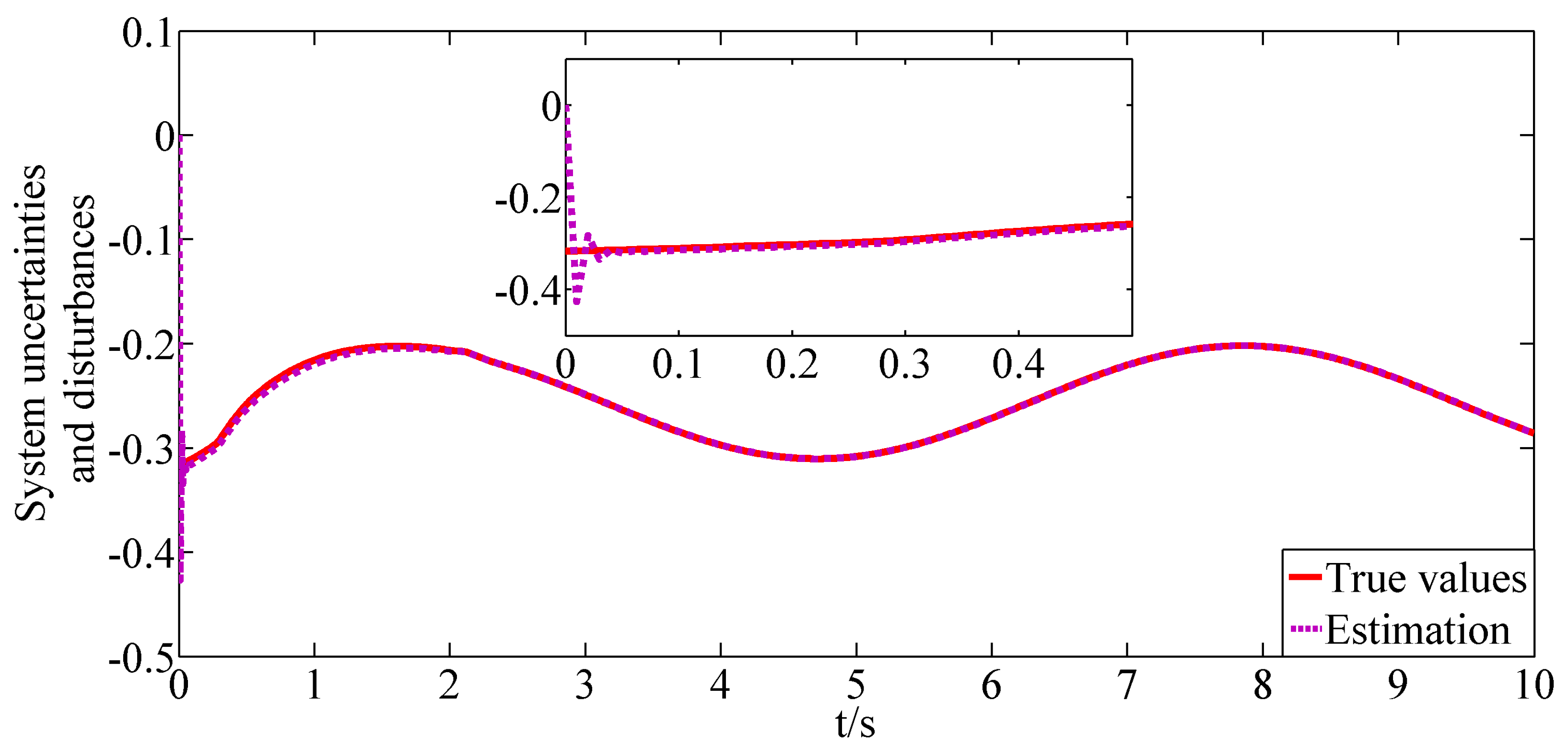
In order to simulate system uncertainties $\Delta f_1\left(\alpha \right)$, $\Delta f_2(\alpha ,q)$, aerodynamic parameter variations are set to 1.1 times the nominal value. The disturbances are given as $d_1=d_2=0.05sint$. NN and NDO are designed as the estimators of the system uncertainties and external disturbances, respectively. 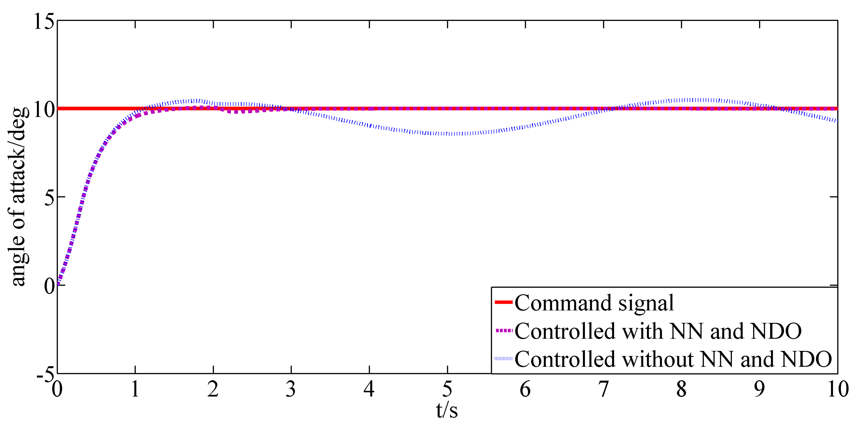In order to illustrate the effectiveness of the NN and NDO, the estimations of the sums of $d_1$, $\Delta f_1\left(\alpha \right)$ and $d_2$, $\Delta f_2(\alpha ,q)$ are shown as Figure 2 and Figure 3, respectively. In addition, the comparison of the response of the angle of attack controlled with and without the designed estimators are shown in Figure 4. As shown in Figure 2 and Figure 3, the system uncertainties and external disturbances can be estimated accurately and quickly under the utility of NN and NDO. From Figure 4, it can be depicted that owing to the designed estimators, the adverse effects caused by the system uncertainties and external disturbances are greatly reduced so that the angle of attack can track the command signal more precisely.

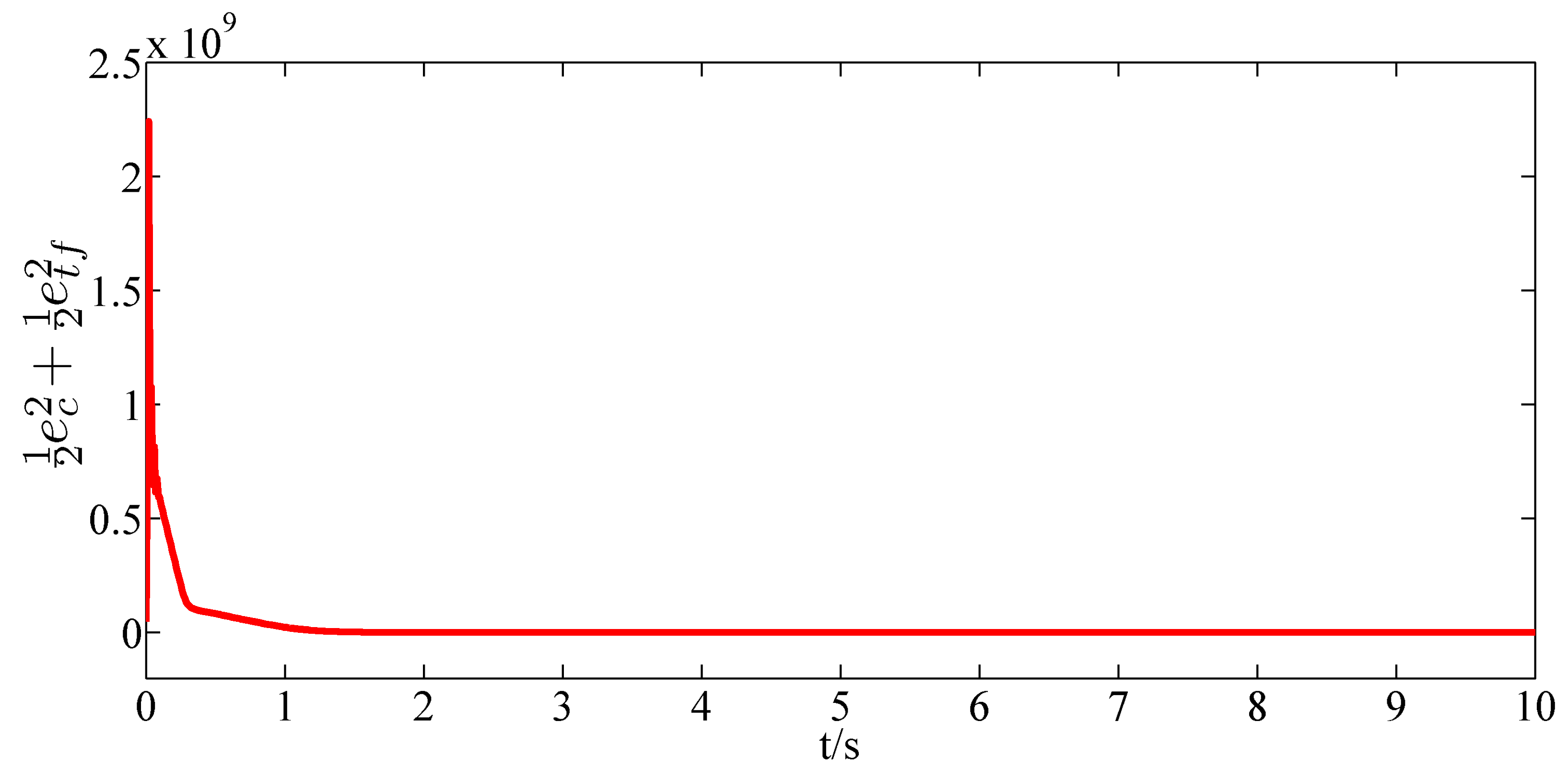
In order to achieve the finite-horizon optimal control, the ADP algorithm is applied. The objective function is given as ${\displaystyle \frac{1}{2}}{e}_c^T{e}_c+{\displaystyle \frac{1}{2}}{e}_{t_f}^T{e}_{t_f}$ in Equation (75). The objective of the ADP algorithm is to minimize the objective function. For the purpose of illustrating the effectiveness of the designed ADP algorithm, the response of ${\displaystyle \frac{1}{2}}{e}_c^T{e}_c+{\displaystyle \frac{1}{2}}{e}_{t_f}^T{e}_{t_f}$ is shown in Figure 5. It can be observed that ${\displaystyle \frac{1}{2}}{e}_c^T{e}_c+{\displaystyle \frac{1}{2}}{e}_{t_f}^T{e}_{t_f}$ gradually decreases and eventually converges to zero. Hence, the designed ADP algorithm is efficient.

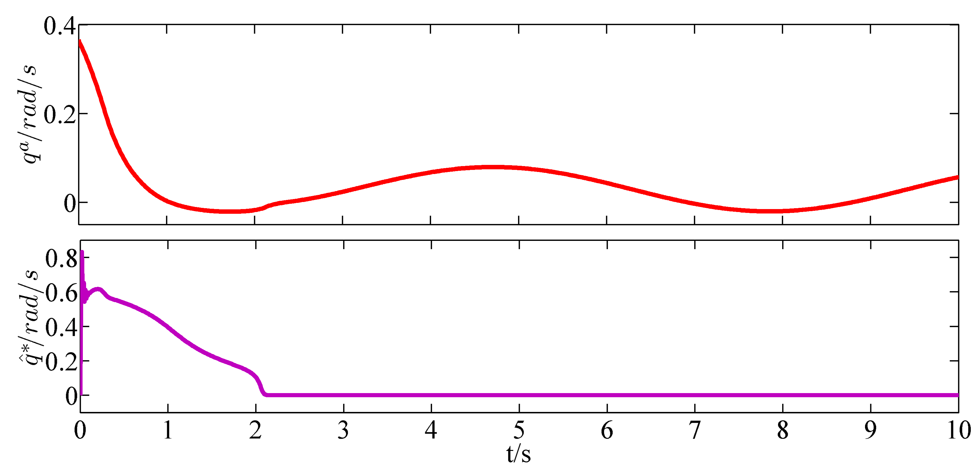
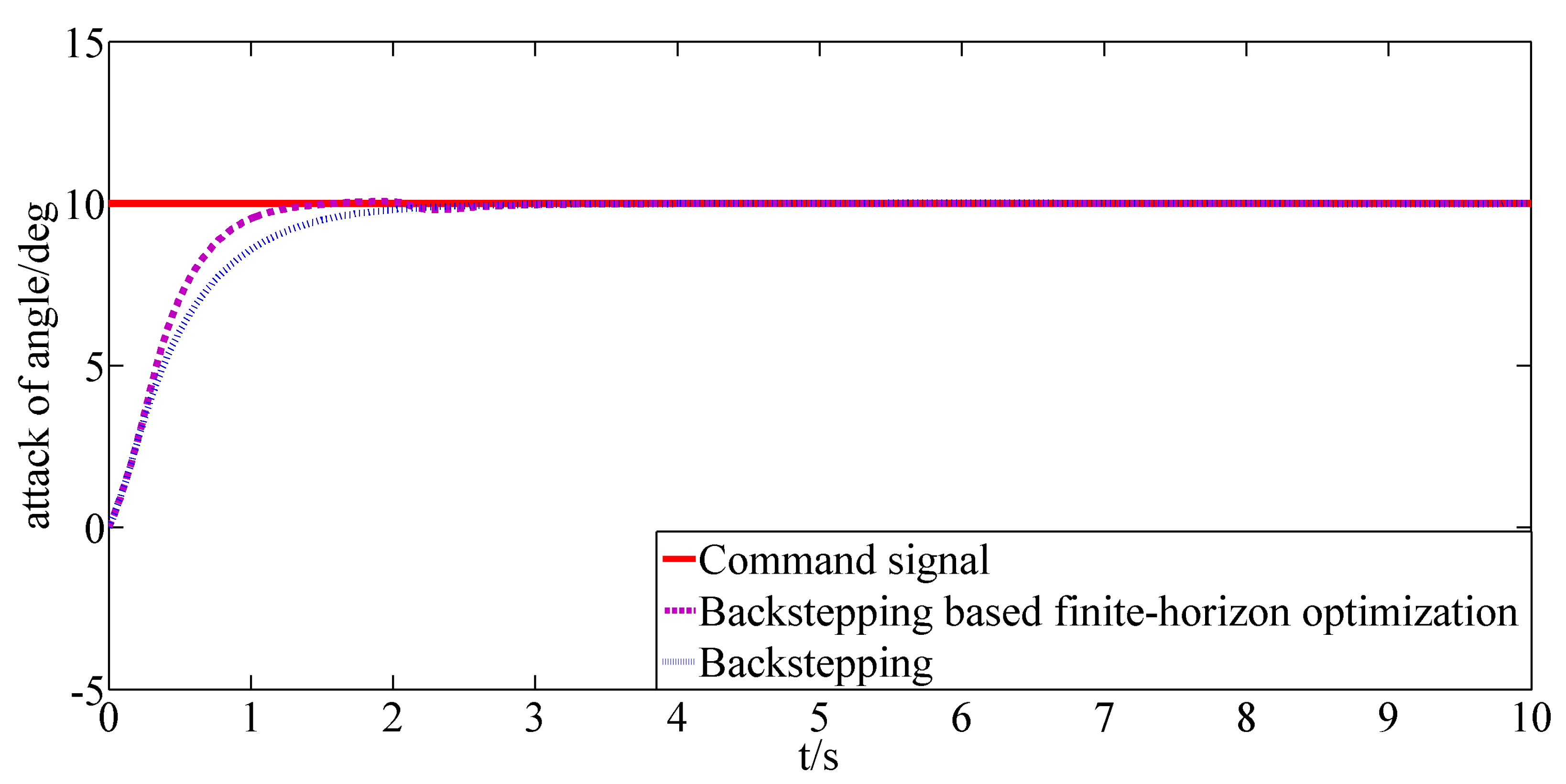
The virtual control inputs $q^a$ defined in Equation (26), the control inputs $u^a$ defined in Equation (36), and ${\widehat{q}}^{*}$ and ${\widehat{u}}^{*}$ defined in Equation (71) are shown in Figure 6 and Figure 7, respectively. Under the action of the backstepping based finite-horizon optimal control inputs, the response of the angle of attack is shown in Figure 8. Furthermore, the response of the angle of attack controlled by the backstepping method with the same parameters is given in Figure 8 as a contrast. It can be illustrated that the system controlled by the designed backstepping based finite-horizon optimal control method can evolve in a finite-horizon optimal way. Thus, the conclusion can be drawn that a better performance can be obtained under the control of the backstepping-based finite-horizon optimal control method.

7. Conclusions

In this paper, a backstepping-based finite-horizon optimal control scheme is proposed to complete the task of angle of attack tracking in a finite-horizon optimal manner. An auxiliary system is designed to compensate for the input constraints. NN and NDO are applied to estimate the system uncertainties and external disturbances. Furthermore, the backstepping method containing NN and NDO is employed to ensure the stability of the system and suppress the adverse effects caused by the system uncertainties and external disturbances. In addition, the DSC technique is utilized to avoid the derivation operation in the process of the backstepping control. Moreover, the ADP algorithm is used to control the system in a finite-horizon optimal manner. In the design of the ADP, a critic NN is constructed by time-state-dependent feature functions to approximate the value function in the HJB equation. Finally, simulation results illustrate the effectiveness of the proposed backstepping-based finite-horizon optimal control scheme.

In future work, a practical experiment will be constructed and carried out to verify the proposed control method.

References

1. Castañeda, H.; Salas-Peña, O.S.; de León-Morales, J. Extended observer based on adaptive second order sliding mode control for a fixed wing UAV. ISA Trans. 2017, 66, 226–232. [Google Scholar] [CrossRef] [PubMed]
2. Lee, C.H.; Chung, M.J. Gain-scheduled state feedback control design technique for flight vehicles. IEEE Trans. Aerosp. Electron. Syst. 2001, 37, 173–182. [Google Scholar]
3. Snell, S.A.; Enns, D.F.; Garrard, W.L. Nonlinear inversion flight control for a supermaneuverable aircraft. J. Guid. Control. Dyn. 1992, 15, 976–984. [Google Scholar] [CrossRef]
4. Lungu, M. Stabilization and control of a UAV flight attitude angles using the backstepping method. World Acad. Sci. Eng. Technol. 2012, 6, 241–248. [Google Scholar]
5. Zhang, J.; Sun, C.; Zhang, R.; Qian, C. Adaptive sliding mode control for re-entry attitude of near space hypersonic vehicle based on backstepping design. IEEE/CAA J. Autom. Sin. 2015, 2, 94–101. [Google Scholar] [CrossRef]
6. Kang, Y.; Chen, S.; Wang, X.; Cao, Y. Deep convolutional identifier for dynamic modeling and adaptive control of unmanned helicopter. IEEE Trans. Neural Netw. Learn. Syst. 2018, 30, 524–538. [Google Scholar] [CrossRef] [PubMed]
7. Wu, D.; Chen, M.; Gong, H.; Wu, Q. Robust backstepping control of wing rock using disturbance observer. Appl. Sci. 2017, 7, 219. [Google Scholar] [CrossRef]
8. Wu, D.; Chen, M.; Gong, H. Robust control of post-stall pitching maneuver based on finite-time observer. ISA Trans. 2017, 70, 53–63. [Google Scholar] [CrossRef] [PubMed]
9. Liu, H.; Lu, G.; Zhong, Y. Robust LQR Attitude Control of a 3-DOF Laboratory Helicopter for Aggressive Maneuvers. IEEE Trans. Ind. Electron. 2013, 60, 4627–4636. [Google Scholar] [CrossRef]
10. Zarei, J.; Montazeri, A.; Motlagh, M.R.J.; Poshtan, J. Design and comparison of LQG/LTR and H controllers for a VSTOL flight control system. J. Frankl. Inst. 2007, 344, 577–594. [Google Scholar] [CrossRef]
11. Bellman, R. Dynamic programming. Science 1966, 153, 34–37. [Google Scholar] [CrossRef] [PubMed]
12. Chanane, B. Optimal control of nonlinear systems: A recursive approach. Comput. Math. Appl. 1998, 35, 29–33. [Google Scholar] [CrossRef]
13. Mracek, C.P.; Cloutier, J.R. Control designs for the nonlinear benchmark problem via the state-dependent Riccati equation method. Int. J. Robust Nonlinear Control 1998, 8, 401–433. [Google Scholar] [CrossRef]
14. Werbos, P. Approximate Dynamic Programming for Real-Time Control and Neural Modeling; Academic Press: New York, NY, USA, 1977. [Google Scholar]
15. Wei, Q.; Song, R.; Yan, P. Data-driven zero-sum neuro-optimal control for a class of continuous-time unknown nonlinear systems with disturbance using ADP. IEEE Trans. Neural Netw. Learn. Syst. 2017, 27, 444–458. [Google Scholar] [CrossRef] [PubMed]
16. Ferrari, S.; Stengel, R.F. Online adaptive critic flight control. J. Guid. Control. Dyn. 2004, 27, 777–786. [Google Scholar] [CrossRef]
17. Ferrari, S.; Steck, J.E.; Chandramohan, R. Adaptive feedback control by constrained approximate dynamic programming. IEEE Trans. Syst. Man Cybern. Part 2008, 38, 982–987. [Google Scholar] [CrossRef] [PubMed]
18. Zhou, Y.; Kampen, E.J.V.; Chu, Q.P. Incremental approximate dynamic programming for nonlinear adaptive tracking control with partial observability. J. Guid. Control. Dyn. 2018, 41, 1–14. [Google Scholar] [CrossRef]
19. Fan, Q.Y.; Yang, G.H. Adaptive actor–critic design-based integral sliding-mode control for partially unknown nonlinear systems with input disturbances. IEEE Trans. Neural Netw. Learn. Syst. 2017, 27, 165–177. [Google Scholar] [CrossRef] [PubMed]
20. Sun, J.; Liu, C. Backstepping-based adaptive dynamic programming for missile-target guidance systems with state and input constraints. J. Frankl. Inst. 2018, 355, 8412–8440. [Google Scholar] [CrossRef]
21. Sun, J.; Liu, C.; Zhao, X. Backstepping-based zero-sum differential games for missile-target interception systems with input and output constraints. IET Control Theory Appl. 2018, 12, 243–253. [Google Scholar] [CrossRef]
22. Xia, R.; Chen, M.; Wu, Q. Neural network based optimal adaptive attitude control of near-space vehicle with system uncertainties and disturbances. Proc. Inst. Mech. Eng. Part J. Aerosp. Eng. 2019, 233, 641–656. [Google Scholar] [CrossRef]
23. Cui, X.; Zhang, H.; Luo, Y.; Zu, P. Online finite-horizon optimal learning algorithm for nonzero-sum games with partially unknown dynamics and constrained inputs. Neurocomputing 2016, 185, 37–44. [Google Scholar] [CrossRef]
24. Cheng, T.; Lewis, F.L.; Abu-Khalaf, M. A neural network solution for fixed-final time optimal control of nonlinear systems. Automatica 2007, 43, 482–490. [Google Scholar] [CrossRef]
25. Zhao, Q.; Xu, H.; Jagannathan, S. Neural network-based finite-horizon optimal control of uncertain affine nonlinear discrete-time systems. IEEE Trans. Neural Netw. Learn. Syst. 2014, 26, 486–499. [Google Scholar] [CrossRef] [PubMed]
26. Sun, J.; Liu, C. Finite-horizon differential games for missile–target interception system using adaptive dynamic programming with input constraints. Int. J. Syst. Sci. 2018, 49, 264–283. [Google Scholar] [CrossRef]
27. Xu, H.; Jagannathan, S. Neural network-based finite horizon stochastic optimal control design for nonlinear networked control systems. IEEE Trans. Neural Netw. Learn. Syst. 2014, 26, 472–485. [Google Scholar] [CrossRef] [PubMed]
28. Chen, M.; Tao, G.; Jiang, B. Dynamic surface control using neural Networks for a class of uncertain nonlinear systems with input saturation. IEEE Trans. Neural Netw. Learn. Syst. 2015, 26, 2086–2097. [Google Scholar] [CrossRef] [PubMed]
29. Abu-Khalaf, M.; Lewis, F.L. Nearly optimal control laws for nonlinear systems with saturating actuators using a neural network HJB approach. Automatica 2005, 41, 779–791. [Google Scholar] [CrossRef]
30. Dierks, T.; Jagannathan, S. Optimal control of affine nonlinear continuous-time systems. In Proceedings of the 2010 American Control Conference, Baltimore, MD, USA, 30 June–2 July 2010; pp. 1568–1573. [Google Scholar]
31. Wang, D.; Liu, D.; Li, H.; Ma, H. Neural-network-based robust optimal control design for a class of uncertain nonlinear systems via adaptive dynamic programming. Inf. Sci. 2014, 282, 167–179. [Google Scholar] [CrossRef]
32. Xu, H.; Zhao, Q.; Dierks, T.; Jagannathan, S. Neural network-based finite-horizon approximately optimal control of uncertain affine nonlinear continuous-time systems. In Proceedings of the 2014 American Control Conference, Portland, OR, USA, 4–6 June 2014; pp. 1243–1248. [Google Scholar]
Figure 1. The control block diagram of the proposed method.
Aerospace 12 00653 g001
Figure 2. The estimations of the sum of d 1 and Δ f 1 ( α ) .
Aerospace 12 00653 g002
Figure 3. The estimations of the sum of d 2 and Δ f 2 ( α , q ) .
Aerospace 12 00653 g003
Figure 4. The response of the angle of attack controlled with and without estimators.
Aerospace 12 00653 g004
Figure 5. The response of the objective function.
Aerospace 12 00653 g005
Figure 6. The response of q a and q * .
Aerospace 12 00653 g006
Figure 7. The response of u a and u * .
Aerospace 12 00653 g007
Figure 8. The response of the angle of attack with and without finite-horizon optimization.
Aerospace 12 00653 g008