Numerical Study of the Late-Stage Flow Features and Stripping in Shock Liquid Drop Interaction

Abstract

Three-dimensional (3D) computational fluid dynamic (CFD) simulations have been performed to investigate the complex flow features and stripping of fluid materials from a cylindrical water drop at the late-stage in a Shock Liquid Drop Interaction (SLDI) process when the drop’s downstream end experiences compression after it is impacted by a supersonic shock wave ($Ma$ = 1.47). The drop trajectory/breakup has been simulated using a Lagrangian model and the unsteady Reynolds-averaged Navier–Stokes (URANS) approach has been employed for simulating the ambient airflow. The Kelvin–Helmholtz Rayleigh–Taylor (KHRT) breakup model has been used to capture the liquid drop fragmentation process and a coupled level-set volume of fluid (CLSVOF) method has been applied to investigate the topological transformations at the air/water interface. The predicted changes of the drop length/width/area with time have been compared against experimental measurements, and a very good agreement has been obtained. The complex flow features and the qualitative characteristics of the material stripping process in the compression phase, as well as disintegration and flattening of the drop are analyzed via comprehensive flow visualization. Characteristics of the drop distortion and fragmentation in the stripping breakup mode, and the development of turbulence at the later stage of the shock drop interaction process are also examined. Finally, this study investigated the effect of increasing $Ma$ on the breakup of a water drop by shear stripping. The results show that the shed fluid materials and micro-drops are spread over a narrower distribution as $Ma$ increases. It illustrates that the flattened area bounded by the downstream separation points experienced less compression, and the liquid sheet suffered a slower growth.

1. Introduction

The disintegration of a liquid drop into tinier fragments is of primary significance for many technological and environmental purposes [1,2,3,4,5], such as internal combustion engines and gas turbines, secondary atomization of liquid jets [6,7], inkjet printing [8,9,10,11], sprays [12,13], and so on. Drop disintegration or secondary atomization is the breakup of larger drops caused by airflows [14]. It represents a very complex multiphase flow challenge because of its extremely unsteady characteristics in both spatial and temporal scales [15,16]. The initial distortion of the drop is initiated by the relative velocity between the drop and the surrounding fluid flow field. This ambient flow field can be achieved due to a sudden acceleration by shock waves, which ultimately leads to drop fragmentation.

The Weber number ($We$) and the Ohnesorge number ($Oh$) are two essential dimensionless parameters applied to classify drop fragmentation. $We$ denotes the ratio of the aerodynamic (inertial) force to the surface tension (capillary) force, while $Oh$ represents the ratio of the liquid viscous force to the surface tension (capillary) force. These two parameters are given as follows:

$$We={\displaystyle \frac{{\rho }_{g,2}{U}_g^{2}d}{{\sigma }_l}},\hspace{1em}Oh={\displaystyle \frac{{\mu }_l}{{\left({\rho }_{l}d{\sigma }_l\right)}^{1/2}}}$$

(1)

where ${\rho }_{g,2}$, ${\rho }_l$, $U_g$, ${\sigma }_l$, ${\mu }_l$, and $d$ denote the post-shock gas density, liquid density, initial gas inflow velocity, liquid surface tension coefficient, liquid dynamic viscosity, and the initial drop diameter, respectively. In early experimental investigations, the liquid drop fragmentation in gaseous flow can generally be categorized into five regimes determined by the initial $We$ [14,17,18]. These regimes are called vibrational, bag, bag-and-stamen/multimode, sheet-thinning/stripping, and catastrophic, with the initial $We$ corresponding to these regimes being ≤12, 12–50, 50–100, 100–350, and >350, respectively [14,17,19]. The vibrational and bag modes have been reported for smaller $Oh$ ($Oh$ < 0.1) [1]. Generally, the vibrational and bag regimes are observed at a small $We$, while the sheet-stripping and catastrophic regimes are well documented at a high $We$ [1]. The bag regime was investigated comprehensively by Theofanous et al. [20], and it was demonstrated that the resulting droplet distribution is bimodal, i.e., the shattering of the bag creates one size, and the capillary breakup of the drop circumference produces larger sizes. Nicholls and Ranger [21] provided a simplified viscous description of the sheet stripping regime without considering the interfacial instabilities and its subsequent roughness. Dai and Faeth [22] assumed that the multi-mode drop fragmentation was a ‘transitional’ regime from bag breakup to sheet-stripping, and appears either as a bag/plume or plume/sheet-stripping breakup. Theofanous et al. [20] explained that the shear or stripping regime developed from $We~{10}^2$ up to $We~{10}^4$ to ${10}^5$, after which the catastrophic or shattering regime sets in as the prevailing mechanism. They showed that the shear or stripping regime entailed a fine mist of liquid originating from the equator, seemingly as a result of a shear-induced boundary layer on the drop surface. Harper et al. [23] provided the first theoretical analysis of the catastrophic regime, and considered it to entail penetration by Rayleigh–Taylor (RT) waves. They claimed that, when $We~{10}^5$, there is a change in behavior from algebraic to exponential for the growth of instabilities. For the different breakup mechanisms for liquid drops impacted by shock waves, the stripping breakup takes place over a broad range of $We$, i.e., $100\le We\le \mathrm{20,000}$ [15]. Theofanous et al. [20] reclassified these five regimes into two competing modes, called the Rayleigh–Taylor Piercing (RTP) and the shear–induced entrainment (SIE). The RTP mode is controlled by the Rayleigh–Taylor instability, where the flattened drop is penetrated by one or more unstable waves, while the SIE regime is mainly due to viscous shearing as well as local disintegrations of the shed filaments resulting from the Kelvin–Helmholtz (KH) instability [24].

Nicholls and Ranger [21] performed the initial experimental investigations of drop breakup by stripping for shock waves in air propagating over a water drop at Mach numbers ($Ma$) ranging from 1.5 to 3.5. They created a model for drop disintegration based on breakup resulting from the boundary-layer stripping mode in which the unstable boundary layer at the drop edge leads to the stripping of the drop fluid. They calculated the breakup rate using the changes in drop shape and velocity coupled with analytical results. Wierzba and Takayama [25] also investigated experimentally the distortion and breakup of liquid drops by stripping. They used holographic interferometry to propose a four-stage stripping disintegration mechanism. The ‘shear stripping’ or ‘boundary-layer stripping’ theory was later corroborated by Chou et al. [26] and Igra et al. [27]. Alternatively, Liu and Reitz [28] suggested another theory, called the sheet thinning mechanism, whereby the inertia drag forces of the ambient gaseous flow results in the production of a thin sheet at the drop border. Joseph et al. [29] carried out similar experiments utilizing a high-speed camera to visualize drop disintegration and the waves produced around different viscous/viscoelastic liquid drops in the airstream behind a supersonic shock wave ($Ma$ = 2 and 3). Chou et al. [26] experimentally investigated changes in drop disintegration characteristics with time in the shear breakup mode using shadowgraphy and holography. Their shadowgraphs showed that ligaments were stripped from the boundary layer at the edge of the deforming drop. They went further to explain that the droplet sizes generated from the disintegration of the ligaments was a function of the liquid viscosity. Hirahara and Kawahashi [30] revealed experimentally that the liquid column distortion time depended on the pressure distribution in the vicinity of the drop as well as the shearing stress induced by drop distortion. Theofanous and Li [31] utilized laser-induced fluorescence to show that the governing mechanism at high $We$ is the shear-induced motion characterized by a major radial component and instabilities on the subsequently produced elongated liquid sheet.

Even though a great amount of detail has been observed from various experimental studies of drop fragmentation, the measurements derived are generally restricted to pictorial information primarily useful for qualitative analysis [32]. This then necessitates the need to conduct quantitative research to verify the different mechanisms presented in the experiments. As a result, numerical simulations are required to augment the experimental studies. Generally, studies have been conducted on the impacts of changing drop size and shock $Ma$ [33], the computation of the characteristic breakup times [19,21,34], and the reliance of breakup dynamics on parameters like density and viscosity ratios of the fluids [18,19,28,29,30,35,36]. One of the earliest numerical simulations to be conducted was the work of Gonor and Zolotova [37]. They developed an analytical technique to investigate drop fragmentation in various $We$. Khosla et al. [38] were one of the first to perform a complete three-dimensional (3D) numerical investigation where they examined the breakup process in the low $We$ mode. Subsequently, more 3D investigations of the drop fragmentation process in the various modes have been conducted assuming an incompressible flow in the RTP regime (Yang et al. [39]) and a completely compressible fluid flow in the SIE mode (Meng and Colonius [40]). Of particular interest is the research work of Meng and Colonius [40], who presented full 3D simulations of the fragmentation of a spherical liquid drop. They ignored viscous and capillary forces in their simulations, as shown by the high $We$ and the low $Oh$ of their numerical setup. Their work analyzed both the fragmentation of the liquid drop and the unsteady flow field whilst presenting the essential function of recirculation zones close to the interface in the sheet-stripping process. Other studies in the literature (e.g., Chen [15]; Aslani and Regele [41]) have carried out more comprehensive physical examinations of the sheet stripping process. Particularly, the experimental setup of Igra and Takayama [42] was applied in the 2D simulations of Meng and Colonius [43] for the fragmentation of a liquid drop in the SIE mode.

These presented experimental and numerical research works have produced several physical models describing the Shock Liquid Drop Interaction (SLDI) process. However, there is scarcely any detailed knowledge available for the complex flow features, such as evolution of an upstream jet and the fragmentation of the deformed drop at the late-stage of the SLDI process. Furthermore, there have been very limited investigations on material stripping from the deformed drop after its downstream end has been compressed at the late-stage of the SLDI process. Thus, the motivation for this study is to investigate numerically the complex flow features as well as the mechanisms for the drop distortion and fragmentation induced by sheet stripping at the late-stage of the SLDI process. Moreover, to the best of our knowledge, no previous studies have addressed the development of turbulence at the late-stage of the SLDI process, which will be elucidated in the current study. Lastly, this paper investigates the effect of increasing the $Ma$ on the disintegration of a water drop by shear stripping.

The remainder of this paper is structured as follows: the methodology employed for this study is described briefly in Section 2; Section 3 presents both quantitative and qualitative comparisons between the numerical predictions and experimental data as well as an elaborate analysis of the instantaneous flow fields to explain the stripping process in the compression phase/later stage of the SLDI process and present the effect of increasing $Ma$ on the breakup of water drop by shear stripping; Section 4 draws the concluding remarks.

2. Numerical Models and Methods

2.1. Mathematical Formulation

The mathematical model consists of three main components:

(1)

Eulerian governing equations for the gas-phase blended with a turbulent model combined with the coupled level-set volume of fluid (CLSVOF) technique using the Ansys Fluent solver.

(2)

Discrete phase modelling (DPM) which employs a Lagrangian model for handling drop tracking and breakup. This model ensures that the location and speed of the drop are tracked promptly by taking into account the distortion of the drop. (1) and (2) are important because the SLDI is based on the simultaneous and consistent characterization of the gas and liquid phases.

(3)

The Kelvin–Helmholtz Rayleigh–Taylor (KHRT) breakup model for describing the disintegration of the liquid drop. The KHRT breakup model is activated in DPM in the Ansys Fluent solver to simulate the atomization process and to track the trajectory of the shed sub-droplets in the airflow.

2.1.1. Eulerian Governing Equations for the Supersonic Airflow

The continuity equation for the gas phase is given as follows [44]:

$${\displaystyle \frac{\partial \rho }{\partial t}}+{\displaystyle \frac{\partial }{\partial x_i}}\left(\rho u_i\right)=0$$

(2)

where $\rho$ and $u_i$ denote the density and mean velocity in the $i^{th}$ direction of the continuous gas phase, respectively, and $x_i$ and $t$ represent the Cartesian coordinate component and physical time.

The momentum equation for the gas phase is given as follows [44]:

$${\displaystyle \frac{\partial }{\partial t}}\left(\rho u_i\right)+{\displaystyle \frac{\partial }{\partial x_j}}\left(\rho u_i{u}_j\right)=-{\displaystyle \frac{\partial p}{\partial x_i}}+{\displaystyle \frac{\partial }{\partial x_j}}\left({\sigma }_{ij}\right)+{\displaystyle \frac{\partial {\tau }_{ij}}{\partial x_j}}+S_F$$

(3)

where $p$ represents the static pressure, $u_i$ and $u_j$ represent the velocity components in the Cartesian coordinate, $S_F$ is the momentum source term induced by the impact of drop movement, ${\sigma }_{ij}$ and ${\tau }_{ij}$ denote the stress tensor, and ${\sigma }_{ij}$, due to molecular viscosity, is defined by Equation (4):

$${\sigma }_{ij}=\left[\mu \left({\displaystyle \frac{\partial u_i}{\partial x_j}}+{\displaystyle \frac{\partial u_j}{\partial x_i}}\right)\right]-{\displaystyle \frac{2}{3}}\mu {\displaystyle \frac{\partial u_k}{\partial x_k}}{\delta }_{ij}$$

(4)

where $\mu$ denotes the dynamic viscosity and ${\tau }_{ij}$ represents the Reynolds stress tensor, which is given as follows:

$${\tau }_{ij}=-\rho \overline{u_i^{\prime }{u}_j^{\prime }}$$

(5)

where $u^{\prime }$ denotes the fluctuating velocity of the gas phase. The Boussinesq approach, which expresses the relationship between the Reynolds stresses and the mean velocity gradients, is used to derive the Reynolds stress term, and is described by Equation (6) [45]:

$$-\rho \overline{u_i^{\prime }{u}_j^{\prime }}={\mu }_t\left({\displaystyle \frac{\partial u_i}{\partial x_j}}+{\displaystyle \frac{\partial u_j}{\partial x_i}}\right)-{\displaystyle \frac{2}{3}}\left(\rho k+{\mu }_t{\displaystyle \frac{\partial u_k}{\partial x_k}}\right){\delta }_{ij}$$

(6)

where ${\mu }_t$ denotes the turbulent (eddy) viscosity respectively, ${\mu }_t$ is estimated in the Turbulence Model section, ${\delta }_{ij}$ denotes the Kronecker delta, i.e., ${\delta }_{ij}=$ 1 if $i=j$, and ${\delta }_{ij}=$ 0 if $i\ne j$, and $k$ represents the turbulent kinetic energy.

The equation of energy conservation for the gas phase is given as follows [44]:

$${\displaystyle \frac{\partial }{\partial t}}\left(\rho E\right)+{\displaystyle \frac{\partial }{\partial x_i}}\left[u_i\left(\rho E+p\right)\right]={\displaystyle \frac{\partial }{\partial x_j}}\left(k_{eff}{\displaystyle \frac{\partial T}{\partial x_j}}\right)+S_h$$

(7)

where $E$ is the total energy, $S_h$ is the energy source term induced by the heat transfer followed by the droplet dispersion, and $k_{eff}$ represents the effective thermal conductivity.

The SLDI process, just like the shock bubble interaction (SBI) process, is predominantly unsteady, and turbulence is generated with usually large-scale unsteady flow structures. Onwuegbu and Yang [46] and Onwuegbu et al. [47] showed that the unsteady Reynolds-averaged Navier–Stokes (URANS) approach was capable of predicting the flow accurately in the SBI process. Since the SLDI process is similar to the SBI process, the same approach, URANS, is adopted in the present study. The URANS equations are derived by averaging Equations (2) and (3), resulting in some extra terms, called Reynolds stresses. These terms need to be computed using a turbulence model. This is presented in detail in the Turbulence Model section.

Turbulence Model

The Reynolds stress model (RSM) represents the most elaborate RANS turbulence model [48,49,50]. As opposed to using the isotropic eddy-viscosity to close the RANS equations, the RSM solves the transport equations for the Reynolds stresses in conjunction with an equation for the rate of dissipation. This results in five extra transport equations for two dimensional (2D) flows and seven extra transport equations for 3D flows. This model thus has an excellent ability to produce precise estimations for complex flows, as it thoroughly considers streamline curvature impacts, swirl, rotation, and rapid strain rate changes. The RSM relies on scale equations, i.e., $\epsilon$-based equations or $\omega$-/baseline (BSL) $\omega$-based equations. For instance, the stress-BSL RSM for modelling the pressure/strain term solves the scale equation derived from the baseline $k$-$\omega$ model, thus helping eradicate the free stream sensitivity noticed with pure $\omega$-based RSMs, such as the stress-omega RSM. The exact form of the Reynolds stress transport equations can be obtained by taking moments of the exact momentum equation. This process involves multiplying and averaging the exact momentum equations for the fluctuations by the fluctuating velocities after which the product is then Reynolds-averaged.

The exact transport equations for the transport of Reynolds stresses, i.e., $\rho \overline{u_i^{\prime }{u}_j^{\prime }}$, are given by Equation (8):

$$\begin{array}{l}\underset{\begin{array}{c}local time\\ derivative\end{array}}{\underbrace{{\displaystyle \frac{\partial }{\partial t}}\left(\rho \overline{u_i^{\prime }{u}_j^{\prime }}\right)}}+\underset{C_{ij}\equiv convection}{\underbrace{{\displaystyle \frac{\partial }{\partial x_k}}\left(\rho u_k\overline{u_i^{\prime }{u}_j^{\prime }}\right)}}\\ =\underset{D_{T,ij}\equiv turbulent diffusion}{\underbrace{-{\displaystyle \frac{\partial }{\partial x_k}}\left[\rho \overline{u_i^{\prime }{u}_j^{\prime }{u}_k^{\prime }}+\overline{p^{\prime }\left({\delta }_{kj}{u}_i^{\prime }+{\delta }_{ik}{u}_j^{\prime }\right)}\right]}}\\ +\underset{D_{L,ij}\equiv molecular diffusion}{\underbrace{{\displaystyle \frac{\partial }{\partial x_k}}\left[\mu {\displaystyle \frac{\partial }{\partial x_k}}\left(\overline{u_i^{\prime }{u}_j^{\prime }}\right)\right]}}\underset{P_{ij}\equiv stress production}{\underbrace{- \rho \left(\overline{u_i^{\prime }{u}_k^{\prime }}{\displaystyle \frac{\partial u_j}{\partial x_k}}+\overline{u_j^{\prime }{u}_k^{\prime }}{\displaystyle \frac{\partial u_i}{\partial x_k}}\right)}}\underset{G_{ij}\equiv bouyancy production}{\underbrace{- \rho \beta \left(g_i\overline{u_j^{\prime }\theta }+g_j\overline{u_i^{\prime }\theta }\right)}}\\ +\underset{{\phi }_{ij}\equiv pressure strain}{\underbrace{p^{\prime }\left({\displaystyle \frac{\partial u_i^{\prime }}{\partial x_j}}+{\displaystyle \frac{\partial u_j^{\prime }}{\partial x_i}}\right)}}-\underset{{\epsilon }_{ij}\equiv dissipation}{\underbrace{2\mu \overline{{\displaystyle \frac{\partial u_i^{\prime }}{\partial x_k}}{\displaystyle \frac{\partial u_j^{\prime }}{\partial x_k}}}}}\underset{F_{ij}\equiv production by system rotation}{\underbrace{- 2\rho {\Omega }_k\left(\overline{u_j^{\prime }{u}_m^{\prime }}{\epsilon }_{ikm}+\overline{u_i^{\prime }{u}_m^{\prime }}{\epsilon }_{jkm}\right)}}\\ +\underset{\begin{array}{c}user-defined\\ source term\end{array}}{\underbrace{S_{user}}}\end{array}$$

(8)

From Equation (8), $C_{ij}$, $D_{L,ij}$, $P_{ij}$, and $F_{ij}$ do not need to be modelled. However, $D_{T,ij}$, $G_{ij}$, ${\phi }_{ij}$, and ${\epsilon }_{ij}$ must be modelled in order to close the equations. For the $\epsilon$-based RSM, $D_{T,ij}$ can be modelled using the generalized gradient-diffusion model of Daly and Harlow [51]:

$$D_{T,ij}=C_s{\displaystyle \frac{\partial }{\partial x_k}}\left(\rho {\displaystyle \frac{k\overline{u_k^{\prime }{u}_l^{\prime }}}{\epsilon }}{\displaystyle \frac{\partial \overline{u_i^{\prime }{u}_j^{\prime }}}{\partial x_l}}\right)$$

(9)

When the turbulent kinetic energy, $k$, is required to model a particular term, as in Equation (9), it is derived by taking the trace of the Reynolds stress tensor, which is shown in Equation (10):

$$k={\displaystyle \frac{1}{2}}\overline{u_i^{\prime }{u}_i^{\prime }}$$

(10)

An alternative for the RSM based on the $\epsilon$-equation is provided by the Ansys Fluent package to solve a transport equation for the turbulent kinetic energy, aiming to derive boundary conditions for the Reynold stresses. In this case, the model equation shown by Equation (11) is used:

$${\displaystyle \frac{\partial }{\partial t}}\left(\rho k\right)+{\displaystyle \frac{\partial }{\partial x_i}}\left(\rho k{u}_i\right)={\displaystyle \frac{\partial }{\partial x_j}}\left[\left(\mu +{\displaystyle \frac{{\mu }_t}{{\sigma }_k}}\right){\displaystyle \frac{\partial k}{\partial x_j}}\right]+{\displaystyle \frac{1}{2}}\left(P_{ii}+G_{ii}\right)-\rho \epsilon \left(1+2M_t^2\right)+S_k$$

(11)

where ${\sigma }_k$ = 1, and $S_k$ denotes a user-defined source term. Equation (11) is essentially derived from contracting the modeled equation for the Reynolds stresses, i.e., Equation (8).

Equation (9) has been simplified to utilize a scalar turbulent diffusivity to prevent numerical instabilities [52]:

$$D_{T,ij}={\displaystyle \frac{\partial }{\partial x_k}}\left({\displaystyle \frac{{\mu }_t}{{\sigma }_k}}{\displaystyle \frac{\partial \overline{u_i^{\prime }{u}_j^{\prime }}}{\partial x_k}}\right)$$

(12)

For the $\omega$-based RSM, the turbulent diffusive transport can be modelled using Equation (12). ${\mu }_t$ is computed by Equation (13):

$${\mu }_t={\alpha }^{*}{\displaystyle \frac{\rho k}{\omega }}$$

(13)

where the coefficient, ${\alpha }^{*}$, is derived by Equation (14):

$${\alpha }^{*}={\alpha }_{\infty }^{*}\left({\displaystyle \frac{{\alpha }_0^{*}+{Re}_t/R_k}{1+{Re}_t/R_k}}\right)$$

(14)

where $R_k=6$, and ${Re}_t$ and ${\alpha }_0^{*}$ are defined as follows:

$${Re}_t={\displaystyle \frac{\rho k}{\mu \omega }};\hspace{1em}\hspace{1em}{\alpha }_0^{*}={\displaystyle \frac{{\beta }_i}{3}}$$

(15)

where ${\beta }_i$ = 0.072.

The value of $\omega$ is computed using the following transport equation and is given by Equation (16):

$${\displaystyle \frac{\partial }{\partial t}}\left(\rho \omega \right)+{\displaystyle \frac{\partial }{\partial x_i}}\left(\rho \omega u_i\right)={\displaystyle \frac{\partial }{\partial x_j}}\left({\Gamma }_{\omega }{\displaystyle \frac{\partial \omega }{\partial x_j}}\right)+G_{\omega }-Y_{\omega }+{D_{\omega }+S_{\omega }+G}_{\omega b}$$

(16)

where $G_{\omega }$ denotes the production of $\omega$, ${\Gamma }_{\omega }$ denotes the effective diffusivity of $\omega$, $Y_{\omega }$ denotes the dissipation of $\omega$ due to turbulence, $D_{\omega }$ denotes the cross-diffusion term, $S_{\omega }$ is a user-defined source term, and $G_{\omega b}$ accounts for buoyancy terms.

This study applied the stress-BSL RSM, which blends the value within the internal region i.e., ${\sigma }_{k,1}$ = 2.0, and the external region, i.e., ${\sigma }_{k,2}$ = 1.0, adopting the blending function, $F_1$. This is shown in Equation (17):

$${\sigma }_k=F_1{\sigma }_{k,1}+\left(1-F_1\right){\sigma }_{k,2}$$

(17)

where $F_1$ denotes the blending function, and is given by Equation (18):

$$F_1=tanh\left({\Phi }_1^4\right)$$

(18)

 ${\Phi }_1$ is given by Equation (19):

$${\Phi }_1=min\left[max\left({\displaystyle \frac{\sqrt{k}}{0.09\omega y}},{\displaystyle \frac{500\mu }{\rho y^2\omega }}\right), {\displaystyle \frac{4\rho k}{{\sigma }_{\omega ,2}{D}_{\omega }^{+}{y}^2}}\right]$$

(19)

 $D_{\omega }^{+}$ is given by Equation (20):

$$D_{\omega }^{+}=max\left[2\rho {\displaystyle \frac{1}{{\sigma }_{\omega ,2}}}{\displaystyle \frac{1}{\omega }}{\displaystyle \frac{\partial k}{\partial x_j}}{\displaystyle \frac{\partial \omega }{\partial x_j}},{10}^{-10}\right]$$

(20)

where y represents the distance to the next surface, and $D_{\omega }^{+}$ denotes the positive part of the cross-diffusion term.

This study also adopted the stress-BSL RSM to model the pressure strain term by solving the scale equation from the BSL $k$-$\omega$ model. This model also ensures that the free stream sensitivity suffered by the stress-omega model is eliminated. This model is also ideal for flows over curved surfaces and a wide range of turbulent flows. It is shown in Equation (21):

$${\phi }_{ij}=-C_1\rho {\beta }^{*}\omega \left[\overline{u_i^{\prime }{u}_j^{\prime }}-{\displaystyle \raisebox{1ex}{$2$}\!\left/ \!\raisebox{-1ex}{$3$}\right.}{\delta }_{ij}k\right]-{\widehat{\alpha }}_0\left[P_{ij}-{\displaystyle \raisebox{1ex}{$1$}\!\left/ \!\raisebox{-1ex}{$3$}\right.}{P}_{kk}{\delta }_{ij}\right]-{\widehat{\beta }}_0\left[D_{ij}-{\displaystyle \raisebox{1ex}{$1$}\!\left/ \!\raisebox{-1ex}{$3$}\right.}{P}_{kk}{\delta }_{ij}\right]-k{\widehat{\gamma }}_0\left[S_{ij}-{\displaystyle \raisebox{1ex}{$1$}\!\left/ \!\raisebox{-1ex}{$3$}\right.}{S}_{kk}{\delta }_{ij}\right]$$

(21)

where $D_{ij}$ is computed as follows:

$$D_{ij}=-\rho \left[\overline{u_i^{\prime }{u}_m^{\prime }}{\displaystyle \frac{\partial u_m}{\partial x_j}}+\overline{u_j^{\prime }{u}_m^{\prime }}{\displaystyle \frac{\partial u_m}{\partial x_i}}\right]$$

(22)

The mean strain rate, $S_{ij}$, is given by Equation (23):

$$S_{ij}={\displaystyle \frac{1}{2}}\left({\displaystyle \frac{\partial u_j}{\partial x_i}}+{\displaystyle \frac{\partial u_i}{\partial x_j}}\right)$$

(23)

${\beta }^{*}$ is as defined by Equation (24):

$${\beta }^{*}={\beta }_i^{*}\left[1+{\zeta }^{*}F\left(M_t\right)\right]$$

(24)

${\beta }_i^{*}$ is given by Equation (25):

$${\beta }_i^{*}={\beta }_{\infty }^{*}\left({\displaystyle \frac{4/15+{\left({Re}_t/R_{\beta }\right)}^4}{1+{\left({Re}_t/R_{\beta }\right)}^4}}\right)$$

(25)

where ${\zeta }^{*}=1.5$, $R_{\beta }=8$, and ${\beta }_{\infty }^{*}=0.09$.

The compressibility function, $F\left(M_t\right)$, is given by Equation (26):

$$F\left(M_t\right)=\left\{\begin{array}{cc}\hfill 0,& M_t\le M_{to}\hfill \\ \hfill M_t^2-M_{to}^2,& M_t>M_{to}\hfill \end{array}\right.$$

(26)

where $M_t^2$ is given by Equation (27):

$$M_t^2={\displaystyle \frac{2k}{a^2}}$$

(27)

and $M_{to}=0.25$ while $a$ is given by Equation (28):

$$a=\sqrt{\gamma RT}$$

(28)

The dissipation of $\omega$ is given by Equation (29):

$$Y_{\omega }=\rho \beta {\omega }^2$$

(29)

$\beta$ is given by Equation (30):

$$\beta ={\beta }_i\left[1-{\displaystyle \frac{{\beta }_i^{*}}{{\beta }_i}}{\zeta }^{*}F\left(M_t\right)\right]$$

(30)

The constants in Equation (21) are as given below:

$${\widehat{\alpha }}_0={\displaystyle \frac{8+C_2}{11}}, {\widehat{\beta }}_0={\displaystyle \frac{8C_2-2}{11}}, {\widehat{\gamma }}_0={\displaystyle \frac{8C_2-2}{11}}$$

(31)

where $C_1$ and $C_2$ are constants with values of 1.8 and 5.2, respectively, ${\delta }_{ij}$ denotes the Kronecker delta, i.e., ${\delta }_{ij}=1$ if $i=j$, and ${\delta }_{ij}=$ 0 if $i\ne j$.

The production terms influenced by buoyancy are modelled as follows:

$$G_{ij}=-\rho \beta \left(g_i\overline{u_j^{\prime }\theta }+g_j\overline{u_i^{\prime }\theta }\right)$$

(32)

where $\overline{u_i^{\prime }\theta }$ is given by Equation (33):

$$\overline{u_i^{\prime }\theta }={\displaystyle \frac{{\mu }_t}{{Pr}_t}}\left({\displaystyle \frac{\partial T}{\partial x_i}}\right)$$

(33)

where ${Pr}_t$ denotes the turbulent Prandtl number for energy with a value of 0.85. Adopting the definition for the thermal expansion coefficient, $\beta$, given by Equation (30), and Equation (32) for ideal gases can be rewritten as follows:

$$G_{ij}=-{\displaystyle \frac{{\mu }_t}{{\rho Pr}_t}}\left(g_i{\displaystyle \frac{\partial \rho }{\partial x_j}}+g_j{\displaystyle \frac{\partial \rho }{\partial x_i}}\right)$$

(34)

The RSM based on the BSL-equation models the dissipation tensor, ${\epsilon }_{ij}$, as follows:

$${\epsilon }_{ij}={\displaystyle \frac{2}{3}}{\delta }_{ij}\rho {\beta }^{*}k\omega$$

(35)

The CLSVOF Two-Phase Flow Model

The continuity equation for the volume fraction of both air and water through the domain can be expressed by the following equations:

$${\displaystyle \frac{\partial \left({\rho }_a{\gamma }_a\right)}{\partial t}}+{\displaystyle \frac{\partial }{\partial x_i}}\left({\rho }_a{\gamma }_a{u}_i\right)=0$$

(36)

$${\displaystyle \frac{\partial \left({\rho }_w{\gamma }_w\right)}{\partial t}}+{\displaystyle \frac{\partial }{\partial x_i}}\left({\rho }_w{\gamma }_w{u}_i\right)=0$$

(37)

where ${\gamma }_a$ and ${\gamma }_w$, represent the volume fraction of air and water in the computational grid cell, respectively. ${\gamma }_a=0$ when the grid cell is totally occupied by water, and ${\gamma }_a=1$ when it is occupied by air. For a grid cell at the interface, ${\gamma }_a$ has a numerical value between 0 and 1, i.e., $0<{\gamma }_a<1$. When there is a jump at the interface, $\rho$ can be defined as follows:

$$\rho ={\gamma }_a{\rho }_a+\left(1-{\gamma }_a\right){\rho }_w$$

(38)

$\mu$ is constant in each fluid but with a jump at the interface, and can be defined as follows:

$$\mu ={\gamma }_a{\mu }_a+\left(1-{\gamma }_a\right){\mu }_w$$

(39)

At the interface, the volume fraction for water can be computed as the sum of both phases adds up to unity, as follows:

$${\gamma }_a+{\gamma }_w=1$$

(40)

As this computational problem involves the generation of vortices and material stripping at the drop interface coupled with the high-density variation between air and water, it is expedient to use an accurate interface tracking technique to capture the drop deformation properly. Several methods are available to track the interface, but most of them often fail to sustain pressure equilibrium for grid cells nearby the interfaces, where two or more fluid components are mixed and struggle to handle large interface distortions, i.e., disintegration and fronts fusing [53]. Onwuegbu and Yang [46] and Onwuegbu et al. [47,54] showed that a coupled level-set and volume of fluid (CLSVOF) model would be able to capture the drop deformation accurately. The level-set (LS) method, which is a popular interface-tracking method for computing two-phase flows with topologically complex interfaces, captures and tracks the interface by the level-set function specified as a signed distance from the interface [55]. However, the level-set method suffers from a deficiency in volume conservation preservation [56]. The VOF, on the other hand, can preserve volume conservation, as it calculates and tracks the volume fraction of a particular phase in each cell instead of the interface itself. However, the computation of the spatial derivatives for the VOF method poses a challenge as the volume fraction of a particular phase is not continuous across the interface. The CLSVOF enables the added sophistication of automatically treating topological alterations with a high degree of accuracy as well as also computing the curvature and normal to the air/water interface. This technique thus boosts a higher accuracy than the standalone LS and VOF models, as it combines their merits and overcomes their deficiencies. Thus, the CLSVOF offers the sophisticated benefits of being discretely conservative at the air/water interface, as it can correctly predict the position of the interface and the shockwaves while these two flow features travel and interact during the numerical computation. Generally, this approach ensures that mass losses are minimized [57], i.e., eradicating numerical errors in the mass conservation of the fluid phases [58], enabling the accurate definition of the interface curvature [58], and preventing the onset of unwanted spurious oscillations/currents at the interface [59,60]. The level-set function, $\phi$, is described as a signed distance to the interface. Following from this, the interface, represented by a zero level-set, $\phi (x,t)$, can be written as $\Gamma =\left\{x|\phi \left(x,t\right)=0\right\}$ in a two-phase flow system. This zero level-set is shown by Equation (41):

$$\phi \left(x,t\right)=\left\{\begin{array}{cc}\hfill +\left|m\right|,& provided x\in the primary phase\hfill \\ \hfill 0,& provided x\in \Gamma \hfill \\ \hfill -\left|m\right|,& provided x\in the secondary phase\hfill \end{array}\right.$$

(41)

where m represents the distance to the interface.

Sussman et al. [61] presented the following form of the governing equations:

$$\rho \left(\phi \right){\displaystyle \frac{\partial \overrightarrow{u}}{\partial t}}+\rho \left(\phi \right)\overrightarrow{u} ·\nabla \overrightarrow{u}=-\nabla p+\nabla ·\mu \left(\phi \right)\left[\nabla \overrightarrow{u}+{\nabla \overrightarrow{u}}^T\right]-\sigma \kappa \left(\phi \right)\delta \left(\phi \right)\overrightarrow{n}\left(\phi \right)$$

(42)

$$\nabla ·u=0$$

(43)

where $\sigma$, $\kappa \left(\phi \right)$, $\overrightarrow{u}$, and $\overrightarrow{n}\left(\phi \right)$ represent the coefficients of surface tension, local mean interface curvature, fluid velocity field, and local unit normal vector on the interface, respectively. The super-index, $T$, denotes the transpose operator, and δ(φ) denotes the Dirac delta function. $\overrightarrow{n}\left(\phi \right)$ and $\kappa \left(\phi \right)$ are expressed as follows:

$$\overrightarrow{n}\left(\phi \right)={\left.{\displaystyle \frac{\nabla \phi }{|\nabla \phi |}}\right|}_{\phi =0};\hspace{1em}\hspace{1em}\kappa \left(\phi \right)=\nabla ·\overrightarrow{n}\left(\phi \right)=\nabla ·\left({\left.{\displaystyle \frac{\nabla \phi }{|\nabla \phi |}}\right|}_{\phi =0}\right)$$

(44)

Equation (42) can then be coupled with the level-set equation for the advection of the level-set function, $\phi$, previously assumed to be a signed distance function, with fluid velocity, $u$. This is presented as follows:

$${\displaystyle \frac{\partial \left(\phi \right)}{\partial t}}+\nabla ·(u_i\phi )=0$$

(45)

where $\phi =0$ represents the interface $\Gamma$. Following from this, the bulk fluid characteristics can be linked to the individual characteristics of each phase, depending on the signed distance function, and is shown as follows:

$$\rho \left(\phi \right)={\rho }_{w}H\left(\phi \right)+{\rho }_a\left(1-H\left(\phi \right)\right)$$

(46)

$$\mu \left(\phi \right)={\mu }_{w}H\left(\phi \right)+{\mu }_a\left(1-H\left(\phi \right)\right)$$

(47)

where $H\left(\phi \right)$ denotes the Heaviside function and is defined by Equation (48):

$$H\left(\phi \right)=\left\{\begin{array}{cc}\hfill 0,& \phi <-\alpha i.e. gas phase\hfill \\ \hfill 1,& \phi >\alpha i.e. liquid phase\hfill \\ \hfill {\displaystyle \frac{1}{2}}\left[1+{\displaystyle \frac{\phi }{\alpha }}+{\displaystyle \frac{1}{\pi }}sin\left({\displaystyle \frac{\pi \phi }{\alpha }}\right)\right],& |\phi |\le \alpha \hfill \end{array}\right.$$

(48)

where $\alpha$ denotes the thickness of the interface on each side. It is also defined as a positive or negative distance from the interface, whose value can be taken to be 1.5 multiplied by the mesh size [62,63]. Sussman et al. [61] also expressed the smoothed realization of the delta function to limit the effects of surface tension within the interface. This function uses zero value in both fluids and is given by Equation (49):

$$\delta \left(\phi \right)={\displaystyle \frac{dH\left(\phi \right)}{d\phi }}=\left\{\begin{array}{cc}\hfill 0,& \left|\phi \right|>\alpha \hfill \\ \hfill {\displaystyle \frac{1}{2\alpha }}\left[1+cos\left({\displaystyle \frac{\pi \phi }{\alpha }}\right)\right],& \left|\phi \right|\le \alpha \hfill \end{array}\right.$$

(49)

2.1.2. Discrete Phase Modelling

Drop Trajectory Equations

Discrete phase modelling was performed employing the one-way Lagrangian model which simulates the continuous phase first before tracking the trajectory of the drop by integrating the force balance on it. This is shown by Equation (50):

$$m_d{\displaystyle \frac{d{u}_{d,i}}{dt}}=f_D$$

(50)

where the subscript ‘$d$’ refers to the drop, and $f_D$ denotes the drag force per unit mass shown by the Stokes drag law as follows:

$$f_D=m_d{\displaystyle \frac{\left(u_i-u_{d,i}\right)}{{\tau }_d}}$$

(51)

where ${\tau }_d$ is the drop response time given by Equation (52):

$${\tau }_d={\displaystyle \frac{{\rho }_d{d}^2}{18\mu }}{\displaystyle \frac{24}{C_{D}Re}}$$

(52)

where $C_D$ denotes the drag coefficient.

Drop Trajectory Integration Schemes

The trajectories of the drop in the discrete phase model are solved iteratively by a stepwise integration over discrete time steps, e.g., the drop velocity is solved by integrating with respect to time at each point along the trajectory. The drop trajectory is approximated by [44]:

$${\displaystyle \frac{dx}{dt}}=u_d$$

(53)

For the sake of simplicity, only a single component is presented in Equation (53). The drop momentum balance provided in Equation (50) can be rewritten in terms of the drag force per unit mass without including extra body forces that may be applied to the drop by external fields such as gravity. This is shown by [44]:

$${\displaystyle \frac{d{u}_d}{dt}}={\displaystyle \frac{1}{{\tau }_d}}\left(u-u_d\right)$$

(54)

The Ansys Fluent solver is used to compute the trajectory by four integration schemes, namely, the Analytic, the Implicit, the Trapezoidal, and the Runge–Kutta. The Analytical and Implicit (first order) schemes are considered lower order and generate fast results as they are one-step methods that are stable at large time steps. However, they tend to be less exact and rely on the size of the timestep for accuracy. The Trapezoidal (second order) and Runge–Kutta (fifth order) are higher order schemes that execute several evaluations of their functions. As a result, they offer higher accuracy than lower order schemes, such as the Euler implicit method. However, as more evaluations between each time step are expected, it increases computational costs. There is also a dependance on a sufficiently small timestep, as very large timestep sizes pose accuracy challenges. Similar computational issues are observed using stiff ordinary differential equations, potentially leading to numerical instability.

To circumvent these challenges, Ansys Fluent provides an automatic drop trajectory integration setting that blends a lower-order and higher-order scheme with an accuracy control, aiming to modify the length scale within a provided error tolerance. This automated tracking scheme applies the Runge–Kutta discretization scheme, as a high order scheme, and the analytical discretization scheme, as a low order scheme, to track the drop very accurately during the optimum time. When the drop is not close to attaining hydrodynamic equilibrium, the higher order scheme is able to reach an accurate solution very rapidly, as it requires less step refinements for a specific tolerance. However, when the drop reaches hydrodynamic equilibrium, the higher order schemes become inadequate, as their step length is restricted to a stable range. This then necessitates the switch to a stable lower order scheme and the facilitation of larger integration steps.

Following from the brief descriptions of the applied integration schemes, an analytical integration can be performed to solve the set of coupled ordinary equations formed by Equations (53) and (54). This leads to Equations (55) and (56) for the new drop velocity $\left(u_d^{n+1}\right)$ and position $\left(x_d^{n+1}\right)$, respectively, and, assuming constant $u$ and ${\tau }_d$. $u_d^{n+1}$ and $x_d^{n+1}$ are given as follows:

$$u_d^{n+1}=u^n+e^{-{\displaystyle \frac{∆t}{{\tau }_d}}}\left(u_d^n-u^n\right)-a{\tau }_d(e^{-{\displaystyle \frac{∆t}{{\tau }_d}}}-1)$$

(55)

$$x_d^{n+1}=x_d^n+∆t{(u}^n+a{\tau }_d)+{\tau }_d\left(1-e^{-{\displaystyle \frac{∆t}{{\tau }_d}}}\right)\left(u_d^n-u^n-a{\tau }_d\right)$$

(56)

where $u_d^n$ and $u^n$ denote the drop and fluid velocity at the previous position.

The explicit Runge–Kutta scheme from Cash and Karp [64] handles the ordinary differential equations as vectors, where the left-hand side is the derivative ${\overrightarrow{y}}^{\prime }$, and the right-hand side is a function $\overrightarrow{f}\left(t,\overrightarrow{y}\right)$, as shown by the following equations:

$${\overrightarrow{y}}^{\prime }=\overrightarrow{f}\left(t,\overrightarrow{y}\right)$$

(57)

and,

$${\overrightarrow{y}}^{n+1}={\overrightarrow{y}}^n+c_1{\overrightarrow{k}}_1+c_2{\overrightarrow{k}}_2+c_3{\overrightarrow{k}}_3+c_4{\overrightarrow{k}}_4+c_5{\overrightarrow{k}}_5+c_6{\overrightarrow{k}}_6$$

(58)

where,

$${\overrightarrow{k}}_1=∆t\overrightarrow{f}\left(t,{\overrightarrow{y}}^n\right)$$

(59)

$${\overrightarrow{k}}_2=∆t\overrightarrow{f}\left(t+a_2∆t,{\overrightarrow{y}}^n+b_{21}{\overrightarrow{k}}_1\right)$$

(60)

$${\overrightarrow{k}}_3=∆t\overrightarrow{f}\left(t+a_3∆t,{\overrightarrow{y}}^n+b_{31}{\overrightarrow{k}}_1+b_{32}{\overrightarrow{k}}_2\right)$$

(61)

$${\overrightarrow{k}}_4=∆t\overrightarrow{f}\left(t+a_4∆t,{\overrightarrow{y}}^n+b_{41}{\overrightarrow{k}}_1+b_{42}{\overrightarrow{k}}_2+b_{43}{\overrightarrow{k}}_3\right)$$

(62)

$${\overrightarrow{k}}_5=∆t\overrightarrow{f}\left(t+a_5∆t,{\overrightarrow{y}}^n+b_{51}{\overrightarrow{k}}_1+b_{52}{\overrightarrow{k}}_2+b_{53}{\overrightarrow{k}}_3+b_{54}{\overrightarrow{k}}_4\right)$$

(63)

$${\overrightarrow{k}}_6=∆t\overrightarrow{f}\left(t+a_6∆t,{\overrightarrow{y}}^n+b_{61}{\overrightarrow{k}}_1+b_{62}{\overrightarrow{k}}_2+b_{63}{\overrightarrow{k}}_3+b_{64}{\overrightarrow{k}}_4+b_{65}{\overrightarrow{k}}_5\right)$$

(64)

The coefficients, $a_{2\dots ..}{a}_6$, $b_{21\dots ..}{b}_{65}$, and $c_{1\dots ..}{c}_6$, are obtained from Cash and Karp [64]. The integration timestep, ∆t, was calculated using Ansys Fluent’s Step Length Factor equation given by Equation (65):

$$∆t={\displaystyle \frac{{∆t}^{*}}{\lambda }}$$

(65)

where $\lambda$ denotes the step length factor, and ${∆t}^{*}$ represents a characteristic time that is related to an approximate time needed for the drop to traverse the mesh cell. In this study, the default value of $\lambda =5$ was set.

KHRT Breakup Model

The KHRT breakup model combines the impacts of KH waves (induced by aerodynamic forces) with RT instabilities (driven by the acceleration of shed micro-drops ejected into the wake region). Micro-drops have been used to describe tiny fragments of fluid materials that have been drawn from the drop peripheries as shock interaction with the water drop progresses. When the supersonic airflow interacts with the liquid drop, surface waves are created on the drop. These surface waves are more obvious on the upstream side of the drop, and lead to the shearing of the drop. As the surface waves evolve, the drop is deformed to generate several liquid ligaments. These liquid ligaments further fragment and disintegrate into smaller fluid droplets. The breakup of the micro-drops which have formed from the initial breakup of the original drop is proportional to the wavelength of the quickest evolving unstable surface wave, $\mathit{\Lambda }$, on the drop. This is given by Equation (66):

$$r_{md}=B_{zero}\mathit{\Lambda }$$

(66)

where $r_{md}$ denotes a characteristic radius of the microdrops, and $B_{zero}$ is a constant with a numerical value of 0.61 [65]. The rate of change of $r_{md}$ with respect to the characteristic radius, $x_d$, of the original drop is expressed by Equation (67):

$${\displaystyle \frac{d{x}_d}{dt}}=-{\displaystyle \frac{\left( x_d-r_{md}\right)}{{\tau }_{RT}}} , r_{md}\le x_d$$

(67)

where ${\tau }_{RT}$ represents the breakup time and is given as follows [44]:

$${\tau }_{RT}={\displaystyle \frac{3.726B_{one}{x}_d}{\mathit{\Lambda }\Omega }}$$

(68)

In Equation (68), $B_{one}$ represents the constant of breakup time, and has a value of 1.73, as proposed by Liu et al. [66]. $\Omega$ represents the maximum growth rate, and is computed as follows [65]:

$$\Omega {\left({\displaystyle \frac{{\rho }_l{x}_d^3}{\sigma }}\right)}^{0.5}={\displaystyle \frac{0.34+0.38{We}_a^{1.5}}{\left(1+Oh\right)\left(1+1.4{Ta}^{0.6}\right)}}$$

(69)

The corresponding wavelength, $\mathit{\Lambda }$, is given as follows [65]:

$${\displaystyle \frac{\mathit{\Lambda }}{x_d}}=9.02{\displaystyle \frac{\left(1+0.45{Oh}^{0.5}\right)\left(1+0.4{Ta}^{0.7}\right)}{{\left(1+0.87{We}_a^{1.67}\right)}^{0.6}}}$$

(70)

In Equations (69) and (70), $Oh$, $Ta$, and ${We}_a$ denote the Ohnesorge, Taylor, and air Weber numbers, respectively. These variables are given as follows:

$$Oh={\displaystyle \frac{{\left({We}_w\right)}^{0.5}}{{Re}_w}},\hspace{1em}\hspace{1em}{We}_a={\displaystyle \frac{{\rho }_{a}d{U}^2}{\sigma }},\hspace{1em}\hspace{1em}Ta=Oh{\left({We}_a\right)}^{0.5}$$

(71)

where ${We}_w$ and ${Re}_w$ denote the water Weber and Reynolds numbers, respectively, while ${\rho }_a$ denotes the air density. These variables are given as follows:

$${We}_w={\displaystyle \frac{{\rho }_{w}d{U}^2}{\sigma }},\hspace{1em}\hspace{1em}{Re}_w={\displaystyle \frac{{\rho }_{w}dU}{{\mu }_w}}$$

(72)

where ${\rho }_w$ and ${\mu }_w$ denote the water density and water dynamic viscosity, respectively. The Rayleigh–Taylor (RT) model is based on wave instabilities on the drop surface, and the frequency of the quickest evolving wave is calculated as follows [44]:

$${\mathsf{\Omega }}_{RT}={\left({\displaystyle \frac{2{\left(-a\left({\rho }_d-{\rho }_a\right)\right)}^{1.5}}{3{\left(3\sigma \right)}^{0.5}\left({\rho }_d+{\rho }_a\right)}}\right)}^{0.5}$$

(73)

where $a$ denotes the acceleration of the drop in the direction of shock propagation, and ${\rho }_b$ is the drop density. The corresponding wave number is computed as follows:

$${\mathrm{K}}_{RT}={\left({\displaystyle \frac{a\left({\rho }_d-{\rho }_a\right)}{3\sigma }}\right)}^{0.5}$$

(74)

During aerodynamic drop disintegration, the breakup pattern is controlled by inertial, viscous, and capillary forces [1]. With respect to the process of drop breakup, $We$ can be used to describe the drop disintegration. Based on Equation (1), $We$ is computed as $3.4\times {10}^4$. This value is relatively high. Since $We$ represents the ratio of the inertial force to the surface tension force, this indicates that the surface tension is negligible. This also proves that the inertial forces control the flow more than the surface tension forces. As a result, surface tension effects can be ignored.

2.1.3. Discretization

The Monotonic Upstream-centered Scheme for Conservation Laws (MUSCL) scheme was used for the spatial discretization of both momentum and continuity equations. This scheme was presented by Van Leer [67], based on the original MUSCL by blending a central difference scheme and a second-order upwind scheme. A first-order implicit scheme was employed for temporal discretization. To achieve numerical stability and accuracy, a very small timestep of $4\times {10}^{-7}$ s was used in the present study with the Courant–Friedrichs–Lewy (CFL) number set as 0.5. The compressive scheme and interface model-based variant was used to discretize the volume fraction equations spatially. This scheme is a second order reconstruction scheme. It was developed from the slope limiters that are used in spatial discretization schemes to inhibit the spurious oscillations or wiggles that would otherwise occur with high order spatial discretization schemes because of sharp alterations in the solution domain [44].

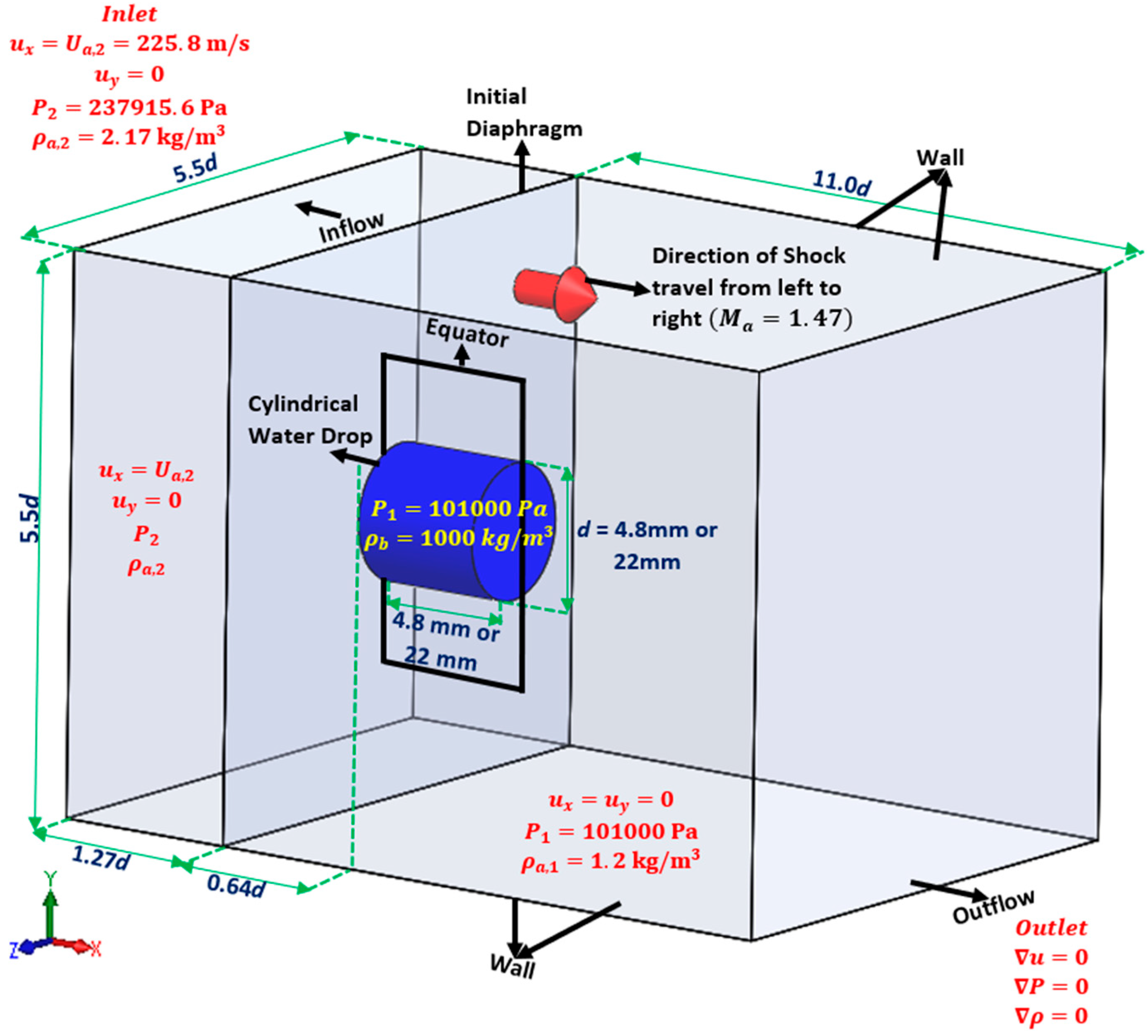
2.2. Computational Details

The computational setup matches the experiments carried out by Igra et al. [27]. The computational domain and the initial/boundary conditions are shown Figure 1 ($x$-axis is horizontal, $y$-axis is vertical, and $z$-axis is spanwise). The length of the computational domain is 12.27 $d$ and both the height and width are 5.5 $d$ ($d$ is the drop diameter, taking 4.8 mm and 22 mm as in the experiments of Igra et al. [27] and Sembian et al. [68], respectively). The no-slip boundary condition is employed on the top, bottom, and side walls. At the outlet boundary, a zero gradient boundary condition is used for all variables. At the inlet, the horizontal velocity component is 225.8 m/s, and both the vertical and spanwise velocity components are zero. Pressure is 237,916 Pa, and density is 2.17 kg/m³. The values of these parameters also denote the post-shock properties of the ambient gas utilized in the initialization, and are calculated from the Rankine–Hugonoit relationships [69]. The initial values in the rest of the computational domain are as follows: velocity is zero, pressure is 1 bar both inside and outside the drop, air density is 1.2 kg/m³, and water density inside the drop is 1000 kg/m³. A sharp interface with interfacial discontinuities is employed. An equator, as seen in Figure 1, is used to explain the material stripping from the deforming drop. The upstream end of the drop is kept at a distance from the incident shock. This is because a shock has a propensity to spread to its normal profile given an ‘exact discontinuity’ as initial conditions which could lead to errors that adversely delay the SLDI process [70].

A hybrid mesh is used in the present study, as shown in Figure 2, which consists of structured uniform hexahedral cells in most of the main region, and smaller uniform hexahedral cells within the drop, while the drop vicinity (just outside and inside) is discretized into ‘smaller-cell’ unstructured triangular prisms. The Cartesian cut-cell method, which was previously applied by Ingram et al. [71], Berger et al. [72], and Johnson [73] has been used to generate this mesh. The unstructured cells used in the drop vicinity enable the local alignment of the grid orientation to the dominant flow direction due to their flexible nature, thus lessening the numerical diffusion, and have been validated by previous works [74,75]. Prior to the application of adaptive mesh refinement (AMR), the cells inside the drop and in its vicinity were made to be finer than the cells in the main flow region. AMR helps to produce a more robust high-resolution grid capable of generating a sharp representation of discontinuities and to adequately resolve the different flow structures under investigation. AMR thus guarantees that the mesh is refined inside the drop and around its vicinity (including the primary shock wave), ensuring that the fine cells surround and travel with the drop. AMR ensures the fine-scale shockwave-droplet interaction close to the interface is effectively resolved. The AMR procedure follows a set of refinement criteria influenced by the physics of the flow solution and the required level of accuracy within the drop and its vicinity. These refinement criteria are based on the gradients of pressure and volume fraction. They result in refinement in regions with high gradients or data density, and coarsening in zones characterized by smooth variations. The AMR procedure is also compatible with the unstructured nature of grid cells shown by the previous works of Lawlor et al. [76], Jahangirian and Shoraka [77], and Cant et al. [78]. They showed that the unstructured grid data enhanced by the AMR approach ensures greater flexibility to treat complex geometries and high-order accuracy. This is possible via the storage of all the neighborhood links between cells based on the local resolution requirements specified by the numerical solution.

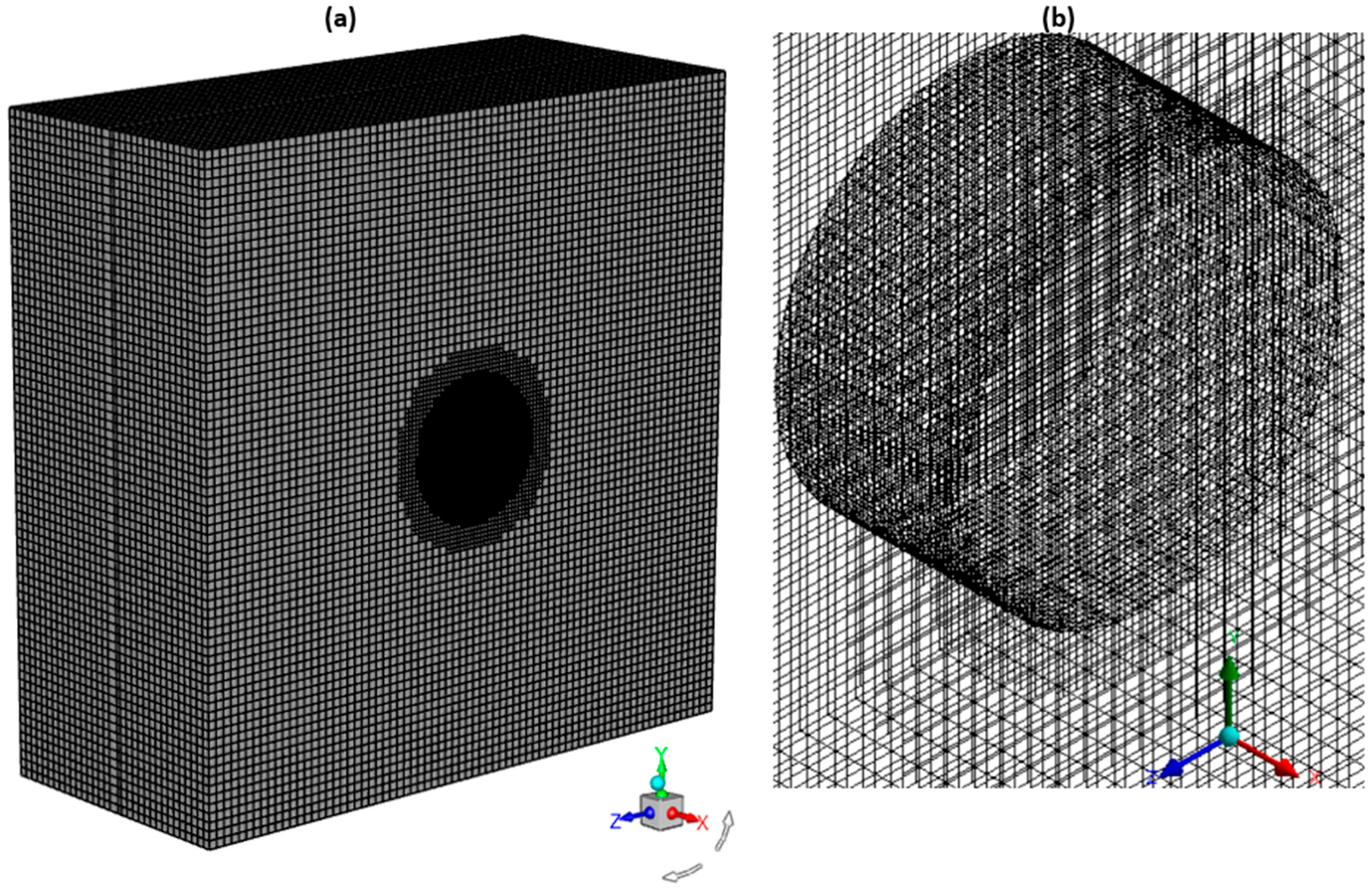
2.3. Mesh Independence Study

A mesh independence study has been conducted with three different qualities of mesh (6.9 million, 10.8 million, and 13.6 million cells) to ensure that the predictions do not depend on the mesh size. This has been presented in Onwuegbu et al. [54], demonstrating that there is hardly any difference between the results obtained from the mesh with 10.8 million cells and the results obtained from the mesh with 13.6 million cells. Hence, there was no need to further refine the mesh, and all computations have been conducted using 13.6 million cells.

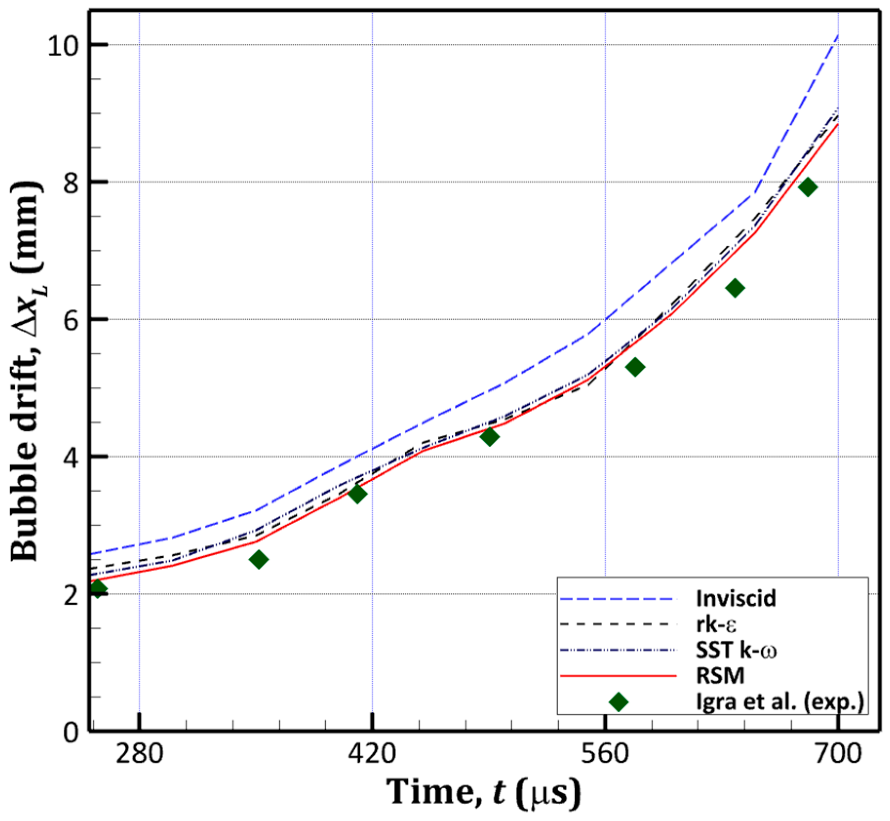
2.4. Turbulence Model Selection

Physical viscosity should be considered if the late-stage turbulence involving small-scale structures and full drop disintegration are to be discussed. This then necessitates the use of turbulence models to effectively study the SLDI phenomenon, as there is hardly any knowledge acquired to date concerning the performance of turbulence models for the SLDI simulations. This study has adopted three extensively applied and highly rated turbulence models: the realizable k-ε, the shear stress transport (SST) k-ω, and a Reynolds stress model (RSM). Their individual performance is very case dependent. Figure 3 shows the comparison between the predicted drop drift with time and the experimental data of Igra et al. [27] for the three turbulence models and the inviscid simulation. The drop leading edge ($x_L$) is important in determining the drop drift, and ${∆x}_L$ is derived as the distance between the current position of $x_L$ and its previous location. At the beginning of the SLDI, $x_L$ is represented by the first position (at the centre of the windward side) that contacts the incident shock wave. It is clearly shown in Figure 3 that the predictions using all three turbulence models show reasonable agreement with the experimental measurements of Igra et al. [27] than the inviscid predictions from the compression phase. This indicates that turbulence is generated after the shock interacts with the drop and turbulence modelling is required to derive more accurate results. It is also clearly seen in Figure 3 that the predictions using all three turbulence models indicate little disparity, but the results from the RSM are marginally closer to the experimental data. Onwuegbu et al. [54] also demonstrated that the RSM provided the closest predictions to the experimental data in the SLDI process. Therefore, the RSM has been adopted in this study.

3. Results and Discussions

For the purpose of comparing our numerical findings with experimental measurements, dimensionless time, $T$, is used and defined as follows:

$$T={\displaystyle \frac{t\times U_{a,2}}{d}}\sqrt{{\displaystyle \raisebox{1ex}{${\rho }_{a,2}$}\!\left/ \!\raisebox{-1ex}{${\rho }_d$}\right.}}$$

(75)

where $U_{a,2}$ and ${\rho }_{a,2}$ denote the post-shock air velocity and post-shock air density, respectively. The authors understand that the presented results reflect a nearly perfect symmetry, which in reality introduce asymmetric vortex shedding and an asymmetric deformed droplet breakup. This could, in turn, lead to the chaotic sideways displacement of the drop and the shed particle clouds. To mitigate potential issues in employing this nearly perfect symmetry, we have focused on ensuring excellent mesh quality and verifying that suitable boundary conditions are employed and interpreted by the Ansys Fluent Solver. The justifications for the mesh generation process, mesh independence study, and the applied boundary conditions have already been presented in the preceding sections. Finally, to mitigate the issues related to a nearly perfect symmetry, we have validated our numerical investigations against experimental data to ensure numerical accuracy and physical facts, as shown in Section 3.1.

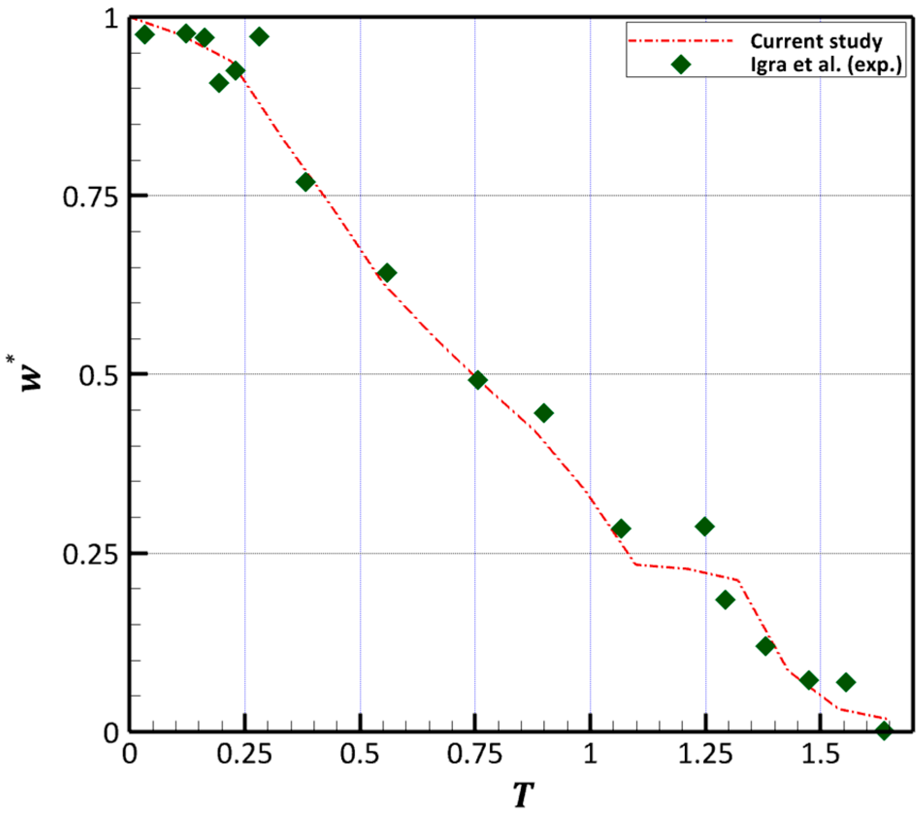
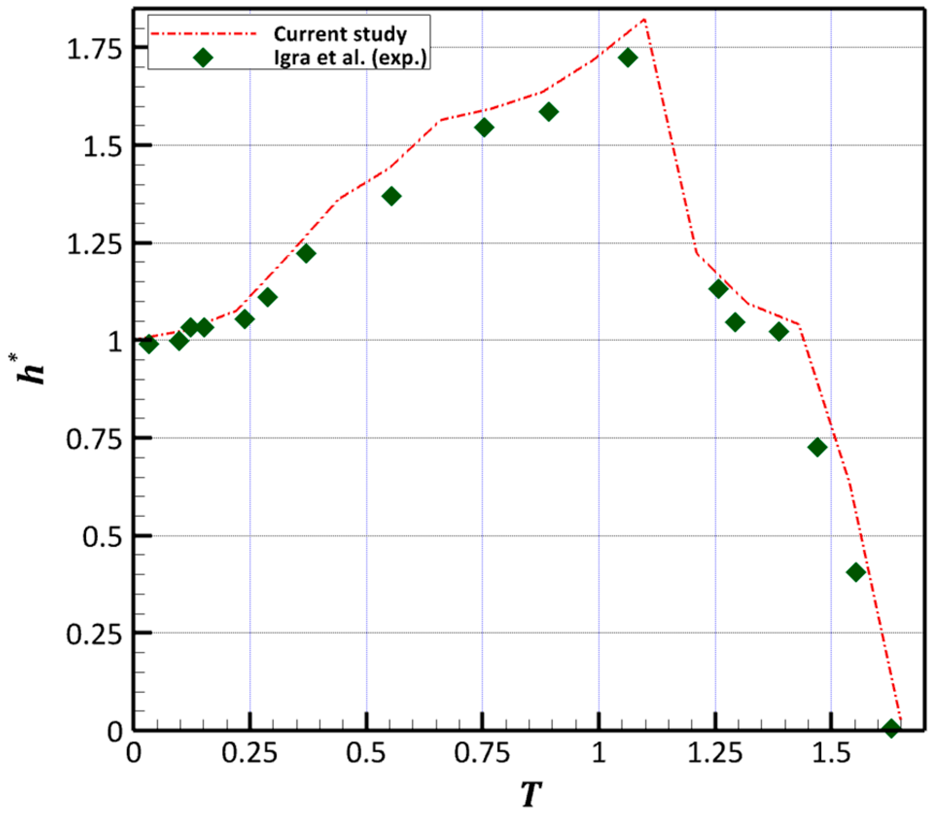
3.1. Predictions of the Temporal Changes of the Interfacial Characteristics Scales

Onwuegbu et al. [54] presented the comparison of the predicted drop trajectory, drag coefficient of the drop, and acceleration at early and intermediate times against the experimental measurements of Igra et al. [27], where a very good agreement was obtained. In the present study, temporal changes in the normalized width ($w^{*}=w/d$) and height ($h^{*}=h/d$) of the deformed drop including the late-stage of the SLDI process are plotted in Figure 4 and Figure 5, where $w$ is derived by measuring the width of the deforming drop in the $x$-direction while $h$ is obtained by measuring its height in the $y$-direction. Areal change ($A$) of the deforming drop has been normalized using the original area of the water drop ($A_o$), i.e., $A^{*}=A/A_o$, and is displayed in Figure 6.

It can be seen clearly from Figure 4 and Figure 5 that a very good agreement between the predictions and the experimental data is obtained. It is also obvious from Figure 4 that the drop width reduces as the SLDI progresses due to drop flattening and stripping of fluid particles from the drop peripheries. The drop width reduction rate varies from the onset of the SLDI to late time. From the onset of the SLDI, the drop width decreases gradually until $T=0.25$. This is then followed by a steep reduction in the drop width until $T=1.05$. Afterwards, the drop width reduces gradually up to $T=1.35$, followed by another steep decrease to $T=1.425$. From $T=1.425$, the decrease in the drop width is less rapid compared to the period between $T=1.35$ and $1.425$ before finishing with a gradual reduction in the drop width. However, the drop height initially increases steadily to $T=1.10$, and then it starts decreasing rapidly at the later stage of the SLDI process, as shown in Figure 5. The initial increase in the drop height is consistent with the lateral stretching of the deforming drop from its top and bottom ends (at the equator) as the drop width reduces due to drop flattening and material stripping.

Figure 6 shows the time variation of the normalized cross-sectional area of the drop, and reveals that the area reduces continuously with time. This is expected because small-sized fluid materials are stripped from the periphery of the drop as the SLDI process progresses. It can be seen from Figure 6 that the predicted temporal changes in drop area are in very good agreement with the experimental data.

It is evident from the above quantitative comparison between the predictions and the experimental data that the numerical approach used in the current study is robust, reliable, and accurate. Further analysis will be presented below to elucidate the materials stripping and other phenomena at the late-stage of the SLDI process.

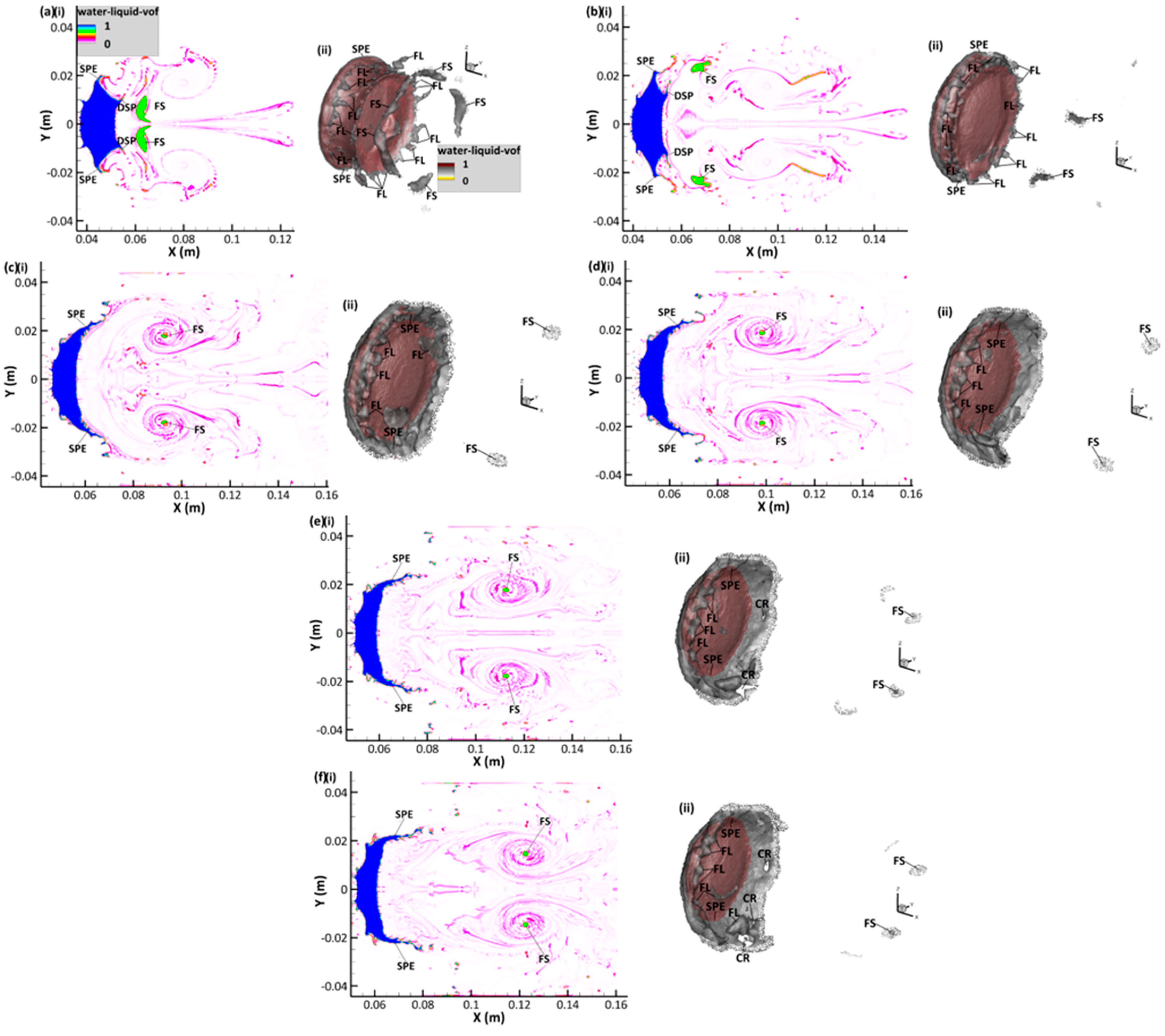
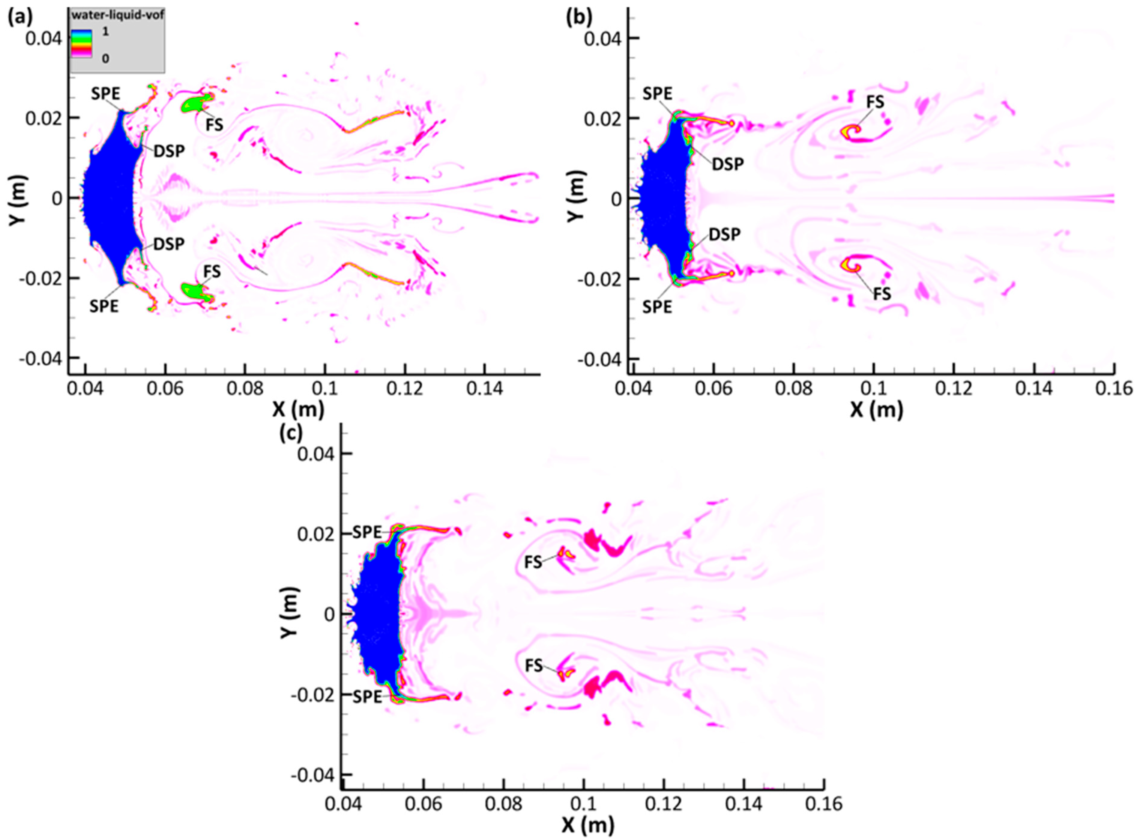
3.2. Stripping and Disintegration of the Liquid Drop

Figure 7a–f(i) display the 2D representations, along the central $x–y$ plane, of small particles (and micro-drops) drawn from the stripping points at the equator (denoted as SPE), and the region succeeding it. It is clearly observable from Figure 7a(i,ii) that a curved, discontinuous fluid sheet (denoted as FS) is entrained from the drop leeward side periphery as a result of strong inertial forces from the surrounding flow. The fluid sheet shown in Figure 7a(i,ii) disintegrates into smaller sheets, as shown in Figure 7b(i,ii), and the fluid particles and micro-drops are transported further downstream from the stripping points at the equator and the drop periphery. It can be seen from Figure 7c(i,ii) that more fluid particles have been drawn from the stripping points at the equator and the drop periphery has undergone more local deformations, as shown by the surface roughness of the drop edges in the vicinity of the equator and around the compressed leeward side. Furthermore, the fluid sheet in Figure 7c(i,ii) has significantly shrunk compared with Figure 7b(i,ii). Figure 7c(i,ii) also shows that the downstream separation points (denoted as DSP in Figure 7a,b(i)) have already fused with the stripping points at the equator with the majority of the fluid shedding now taking place around the stripping points at the equator.

Figure 7a,b(ii) show that fluid ligaments (denoted as FL) are formed around the leeward side of the drop periphery, and the fluid ligaments gradually break into smaller ligaments and micro-drops, as shown in Figure 7c–f(ii). Moreover, Figure 7b–f(i) show that the entire wake region is characterized by a chaotic, turbulent-like flow, and as fluid materials are shed and entrained from the drop, it is visible in the wake region as a spray. This is concordant with the works of Harper et al. [23]. Following from this, Figure 7d–f(ii) show that the bowl-shaped liquid sheet has lost its coherent structure, and the growth of instabilities on the liquid sheet are characterized by the evolution and subsequent fragmentation of the fluid ligaments. Figure 7d–f(ii) also show that these instabilities are located at the stripping points at the equator and the peripheries of the deformed sheet. This is due to the aerodynamic force caused by the high-speed gas flow in its vicinity, piercing or rupturing its sides. This yields more fluid ligaments which remain attached at first but later detach and are propagated downstream. This piercing or rupturing effect creates the crevices (denoted as CR) observed in Figure 7e,f(ii).

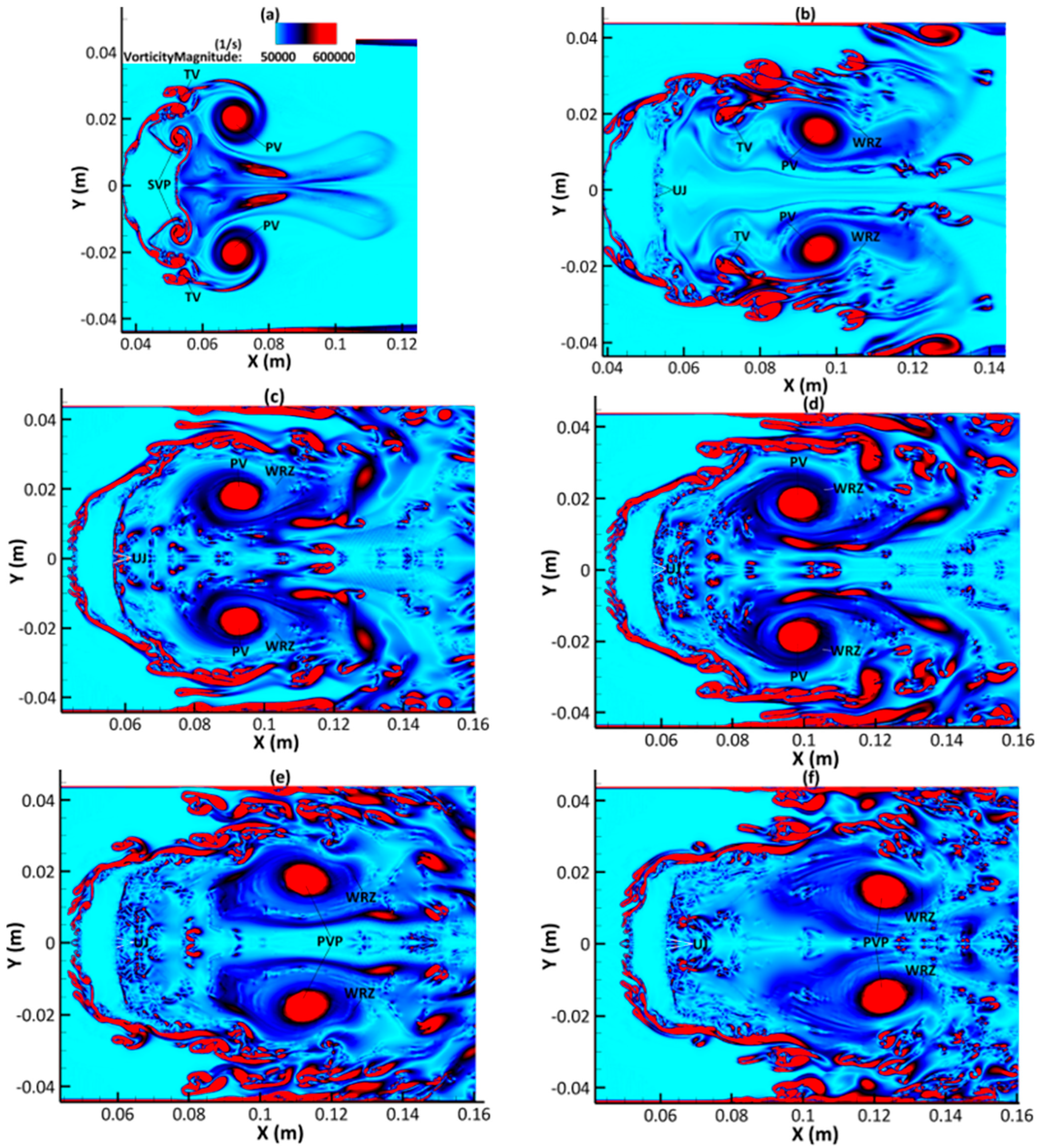
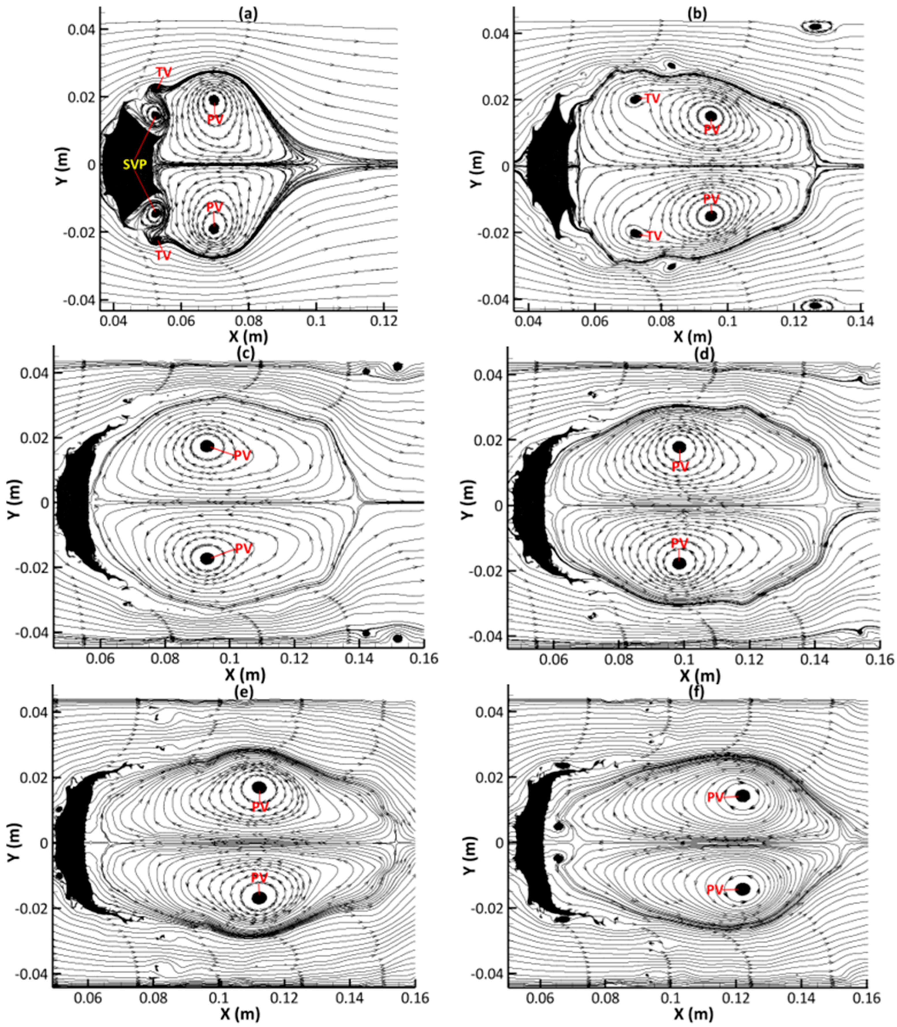
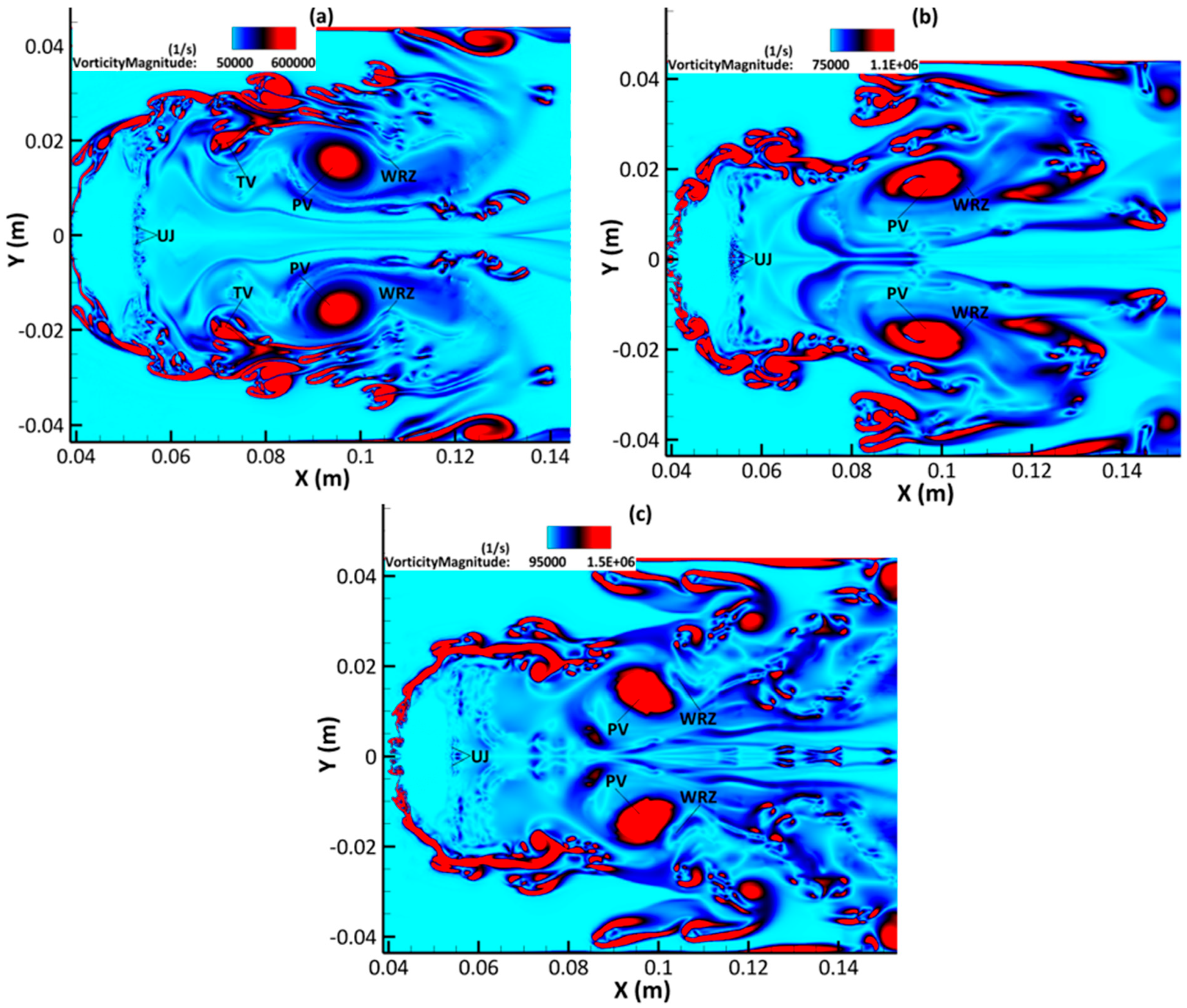
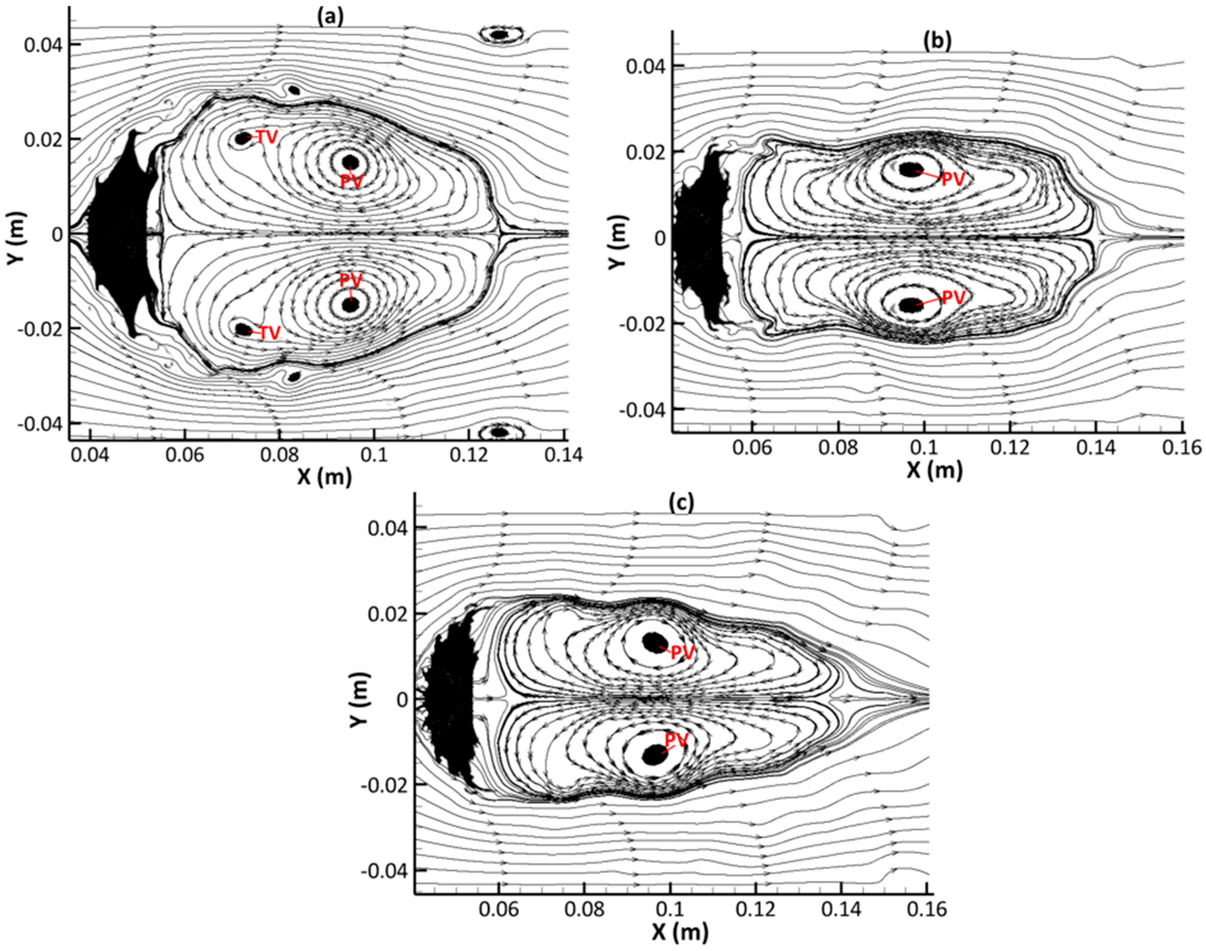
3.3. Dynamics of Vorticity Generation and Evolution

Vorticity generation and deposition represents one of the most important flow phenomena in the SLDI process. Baroclinic torque, which occurs when the shock wave interacts with the perturbed interface [79], leads to the deposition of vorticity on the interface shortly after shock propagation. This is due to the misalignment of the density gradient across the interface and the pressure gradient created by the shock wave [79,80]. As the shock wave propagates through the drop, vorticity is produced and transported in the flow, as shown in Figure 8. Figure 8a shows that one primary vortex (denoted as PV) at the top and another one at the bottom have been generated, which are rotating in different directions. Figure 8a also shows a secondary vortex pair (denoted as SVP) with each secondary vortex rotating in a different direction opposite to the primary vortex. In addition, one tertiary vortex (denoted as TV) at the top and another one at the bottom are also clearly observable in Figure 8a.

The complex flow features in the wake region are due to the generation and quick evolution of those three vortex systems, and the second vortex pair cannot be observed anymore in Figure 8b at $T=0.45$, while the primary and tertiary vortices are still clearly visible. As the SLDI progresses, the tertiary vortex also disappears, and is not visible in Figure 8c at $T=0.53$. By contrast, the primary vortex is persistent, and still clearly visible in Figure 8f at $T=0.68$. When the primary vortex pair is shed, it results in the formation of a wake recirculation zone (denoted as WRZ), as shown in Figure 8b, which drags the ambient fluid materials into a jet travelling upstream (denoted as UJ) that impinges on the leeward side of the drop. This upstream jet contributes to the subsequent flattening/compression of the drop, and its effects on the leeward side of the deformed drop are clearly shown in Figure 9, which cause the hollowing of the leeward side, and the deformed drop looks like a bowl. Furthermore, the jagged edges of the deformed sheet in Figure 9 strongly indicate that a substantial amount of material has been dragged off the edges of the severely deformed drop at the late-stage of the SLDI process. It is worth noting that, at the late-stage of the SLDI process, vorticity is present in most of the wake region with a lot of small-scale flow structures generated, as shown in Figure 8d–f, suggesting that turbulent flow is developed in the wake region.

Figure 10a presents the streamlines on the central $x–y$ plane, showing the rotation directions of the three vortex systems (primary, secondary, and tertiary vortex), and it can be seen clearly that the top primary vortex spins in the clockwise direction while the bottom one spins in the reverse direction, leading to the formation of the upstream jet discussed above. Figure 10a reveals that the tertiary vortex spins in the same direction as the primary vortex, whereas the secondary vortex rotates in the opposite direction. It is also observable that the tertiary vortex, as shown in Figure 10a,b, and the primary vortex, as shown in Figure 10a–f, maintain their direction of rotation as they travel downstream. It can also be confirmed from Figure 10 that the secondary vortex has a much shorter life span and disappears quickly, followed by the tertiary vortex, whereas the primary vortex is persistent and still clearly visible in Figure 10f. Moreover, as can be seen from Figure 10d–f, the tip of the deformed drop is significantly stretched with more materials being stripped from the tip, leading to the formation of small-scale flow structures, as mentioned above.

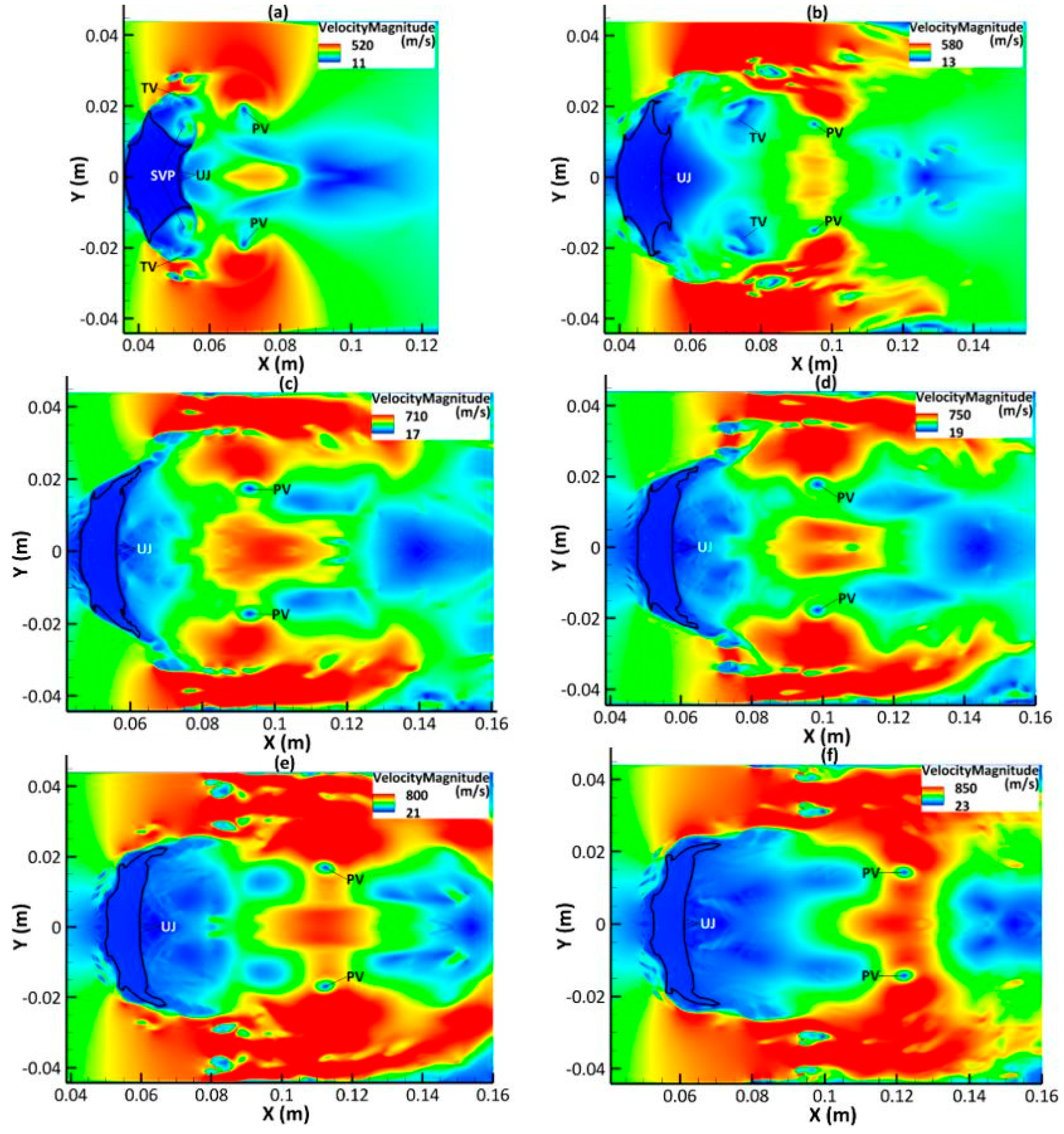
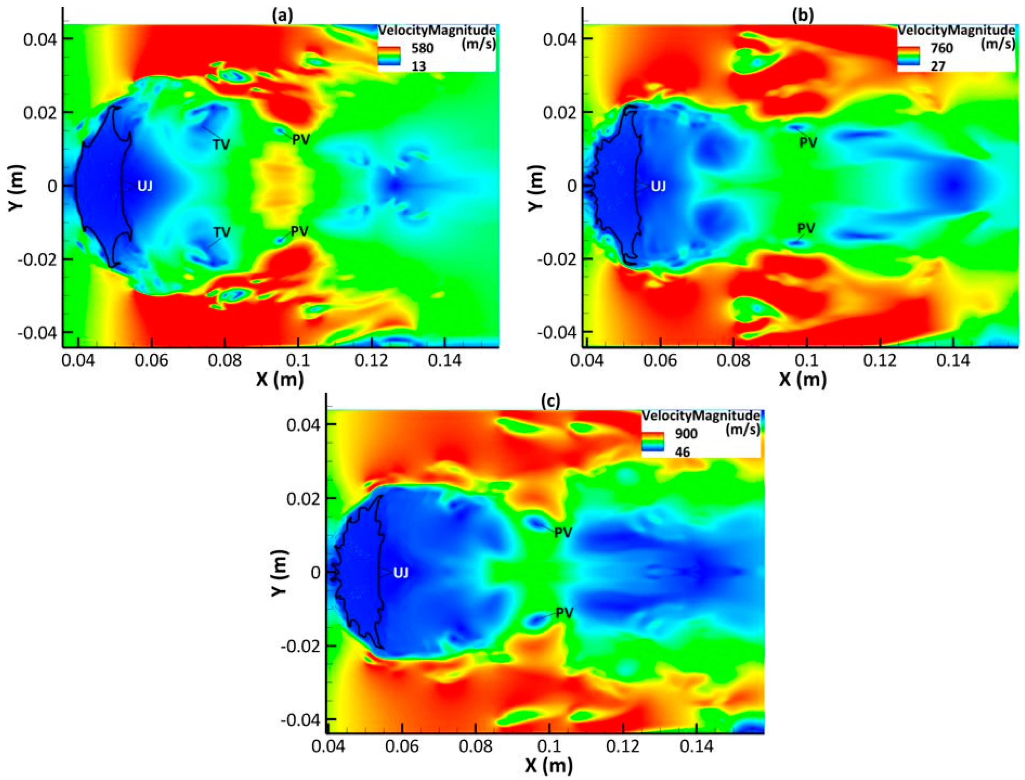
3.4. Velocity Distribution

Figure 11 presents snapshots of velocity magnitude contours on the central $x–y$ plane, showing a very complex velocity field around the deformed drop. Figure 11 also provides an insight into the aerodynamic shock pressure/velocity fronts upstream and downstream of the drop. This is because it reveals the velocity at which the shock wave propagates behind the drop, across the drop, and sections of the shock tube ahead of the drop. It is clearly observable that the high velocity regions are mainly at the top and bottom of the deformed drop, and the low velocity regions are in the wake area. Figure 11a shows that there is a small central relatively high velocity zone, indicating that the upstream jet is just formed and subsequently grows larger and stronger, as shown in Figure 11b–f. The upstream jet has the highest velocity in the region between the top and bottom primary vortices, and the jet velocity starts to reduce further, eventually impinging on the leeward side of the deformed drop at a lower velocity. When the primary vortices travel downstream, the upstream jet may just about impinge on the leeward side of the severely deformed drop, as shown in Figure 11e. The upstream jet may not directly impinge on the leeward side when the primary vortices travel further downstream, as shown in Figure 11f, which can be confirmed from the streamlines in Figure 10f, further showing that the upstream jet does not impinge directly on the surface.

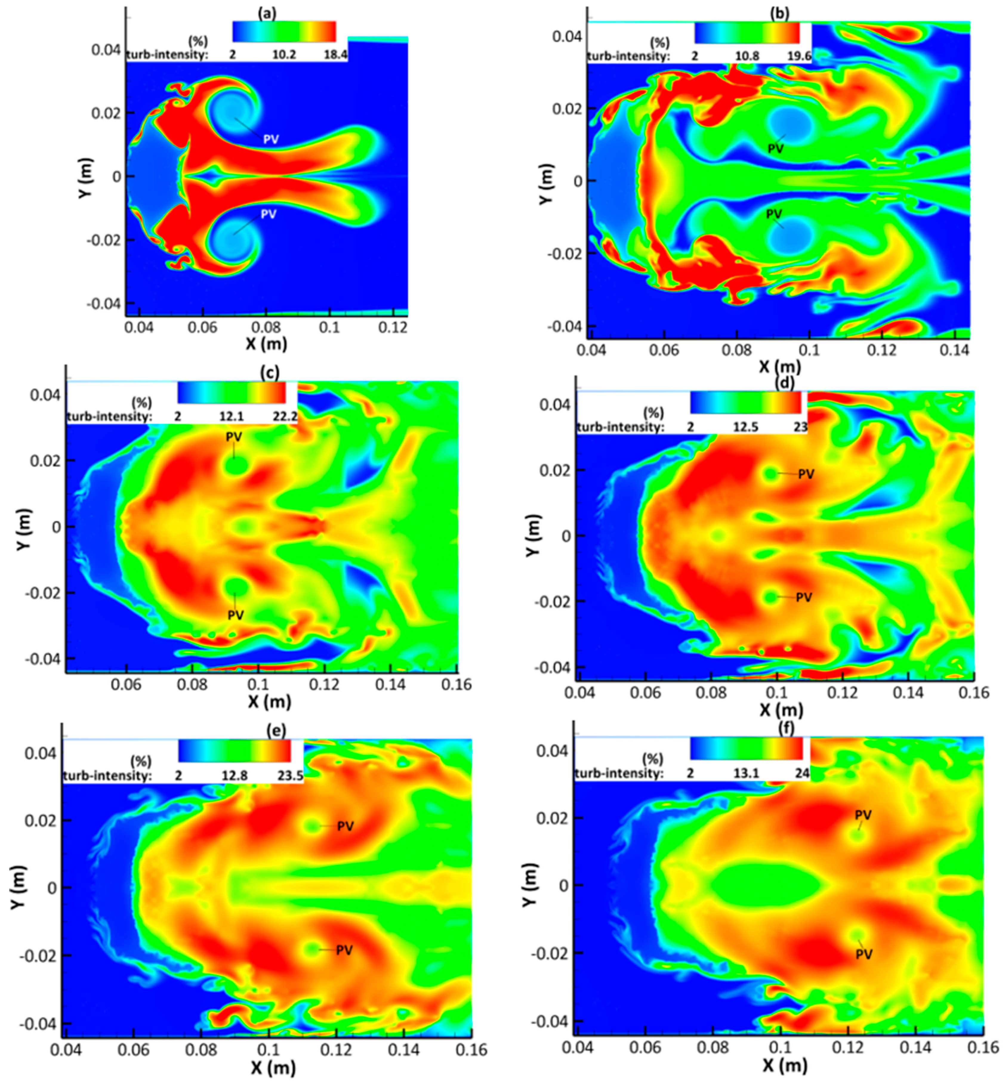
3.5. Turbulence Development

Turbulence development at the late-stage of the SLDI process has been rarely studied in previous works. Figure 12 presents the contours of turbulence intensity along the $x–y$ plane. Turbulence intensity in the present study is defined as follows [44]:

$$\mathrm{turb}\text{-}\mathrm{intensity}={\displaystyle \frac{100}{U}}\sqrt{{\displaystyle \raisebox{1ex}{$2k$}\!\left/ \!\raisebox{-1ex}{$3$}\right.}}$$

(76)

where U and k represent the streamwise velocity and turbulent kinetic energy, respectively.

It has been demonstrated in our previous study [54] that turbulence starts to be generated at quite an early stage ($T=0.12$) even before the drop is deformed, and it can be seen from Figure 12a that significant turbulence has been generated in the area surrounding the deformed drop leeward side at $T=0.37$, with the maximum turbulence intensity reaching about 18.4%. There is a large, continuous high turbulence intensity region in the wake area, as shown in Figure 12a; whereas, at $T=0.45$, after the primary vortex shedding (denoted as PV), this large region has been broken into many smaller areas located in the shear layer regions, as shown in Figure 12b, with the maximum value of turbulence intensity increasing slightly to 19.6%. The complex flow field downstream of the deformed drop changes rapidly, leading to a rapid expansion of those smaller high turbulence intensity areas, as shown in Figure 12c at $T=0.53$. It can be seen from Figure 12d that the high turbulence intensity areas spread further at $T=0.60$ and occupy most of the near wake region with the maximum turbulence intensity reaching about 23%, indicating that it is fully developed turbulent flow in this region. Afterwards, the high turbulence intensity region seems to move downstream, and is mainly concentrated in the far wake region at $T=0.68$, as shown in Figure 12f, along with the maximum turbulence intensity rising to 24%.

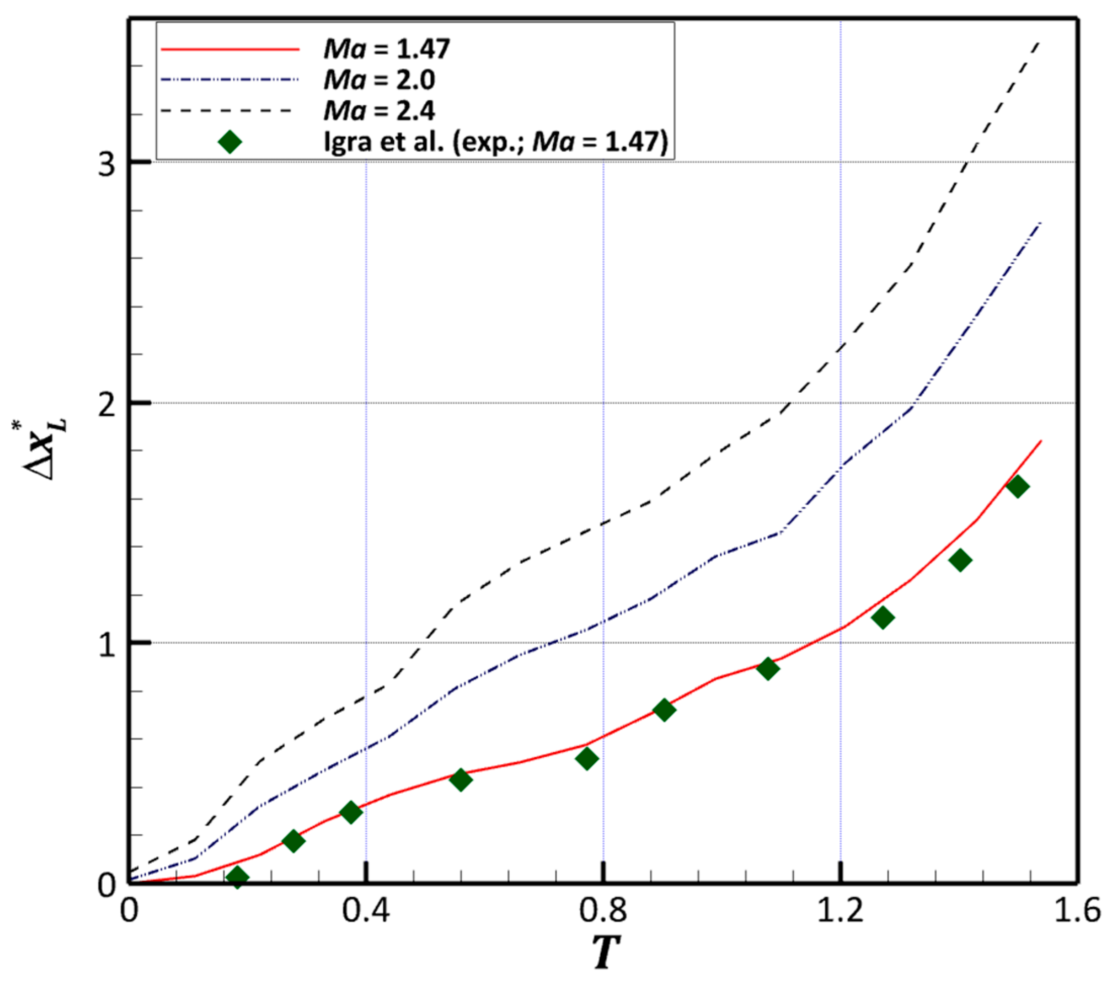
3.6. Effect of Mach Number on the Stripping Breakup of a Water Drop

This section investigates the impact of increasing $Ma$ on the aerobreakup of a water drop after it is impacted by a planar shock wave of varying strengths. The disintegration of a cylindrical water column for the $Ma$ = 1.47 case has already been presented. Two additional cases are then investigated, i.e., $Ma$ = 2.0 and $Ma$ = 2.4, after which the results are presented for the trajectory of the dimensionless streamwise drift of the distorted drop with time for the three $Ma$ cases as the SLDI progresses. The fragmentation of the water drop is also presented at $T$ = 0.45 for the three $Ma$ scenarios that are investigated numerically using contours of volume fraction, vorticity, velocity, pressure, and turbulent intensity on the central $x–y$ plane. The parameters for these simulations are shown in

Table 1. Set-up parameters for the numerical simulation scenarios.

	Pre-Shock Air Properties	Post-Shock Air Properties			Water
		$\mathit{M}\mathit{a}\mathbf{=}\mathbf{1.47}$	$\mathit{M}\mathit{a}\mathbf{=}\mathbf{2.0}$	$\mathit{M}\mathit{a}\mathbf{=}\mathbf{2.4}$
$\rho (\mathrm{k} \mathrm{g}{\mathrm{m}}^{-3})$	1.2	2.17	3.19	3.84	1000
$u (\mathrm{m} {\mathrm{s}}^{-1})$	0	225.8	428.9	567.1	0
$p \left(\mathrm{M}\mathrm{P}\mathrm{a}\right)$	0.101	0.24	0.45	0.66	0.101

. From Table 1, $\rho$, $u$, and $p$ denote density, velocity, and pressure respectively.

Values of $We$ corresponding to the respective $Ma$ are $3.4\times {10}^4$ ($Ma$ = 1.47), $17.8\times {10}^4$ ($Ma$ = 2.0), and $37.4\times {10}^4$ ($Ma$ = 2.4). The $We$ has been obtained from Equation (1) using the density and velocity of the shocked gas for $Ma$ = 2.0 and $Ma$ = 2.4, as provided in Table 1, while the initial diameter of the water drop and the surface tension coefficient remain unchanged. The computed values of $We$ show a direct relationship with $Ma$. Therefore, the arguments provided for the effects of increasing $Ma$ on the aerobreakup of the water drop in the following discussions also apply for the impact of increasing $We$ on the shear stripping of the water drop.

Figure 13 shows the changes in the drift of the distorted drop, ${∆x}_L$, normalized by the initial column diameter ($d$), i.e., ${∆x}_L^{*}={∆x}_L/d$, for the three $Ma$ cases as time progresses. The drop drift provides a clear history of the drop travel as it is deformed. From Figure 13, it is clear that as $Ma$ increases, the distorted drop travels faster. The experimental results for Igra et al. [27] are also presented in Figure 13 for the case of $Ma$ = 1.47. It shows that their result is concordant with the current study for $Ma=$ = 1.47.

Figure 14 shows the volume fraction contours along the central $x–y$ plane for the three $Ma$ cases. Figure 14 describes the shedding of small fluid materials, particles, and micro-drops from the stripping points at the equator and the drop periphery. Figure 14 also reveals the position of the curved, discontinuous fluid sheet, which has been dragged from the drop downstream edge due to strong inertial forces created by the ambient flow.

Figure 14b,c show that the fluid sheet has travelled a significantly greater distance compared to that in Figure 14a. The fluid sheet in Figure 14c has also undergone the most disintegration compared to that in Figure 14b, while the fluid sheet in Figure 14a has suffered the least disintegration. Also, Figure 14b shows that the downstream separation point (DSP) appears closer to the stripping points at the equator (SPE) compared to Figure 14a. However, Figure 14c shows that the downstream separation points have already fused with the stripping points at the equator, and most of the fluid shedding now occurs at the stripping points at the equator. Very interestingly, as $Ma$ increases, the flattening of the downstream end of the liquid sheet becomes weaker due to the declining pressure distribution around the region bounded by the downstream separation points and its immediate environs, i.e., near the wake area. Similar patterns have been reported in the experimental measurements of Karyagin et al. [81] and Nagata et al. [82]. Also, as $Ma$ increases, the lateral stretching of the liquid sheet, from its top and bottom ends (at the equator), is reduced. This study has linked this observation to the experimental findings of Theofanous et al. [35] and Papamoschou and Roshko [83] as well as the numerical investigations of Jalaal and Mehravaran [84]. The works of Theofanous et al. [35] and Jalaal and Mehravaran [84] explained that the evolution of the liquid sheet is enhanced by the appearance of travelling waves on the surface of the drop generated by the Kelvin–Helmholtz instabilities at the upstream end where the liquid/gas interface is subjected to strong shear. The waves are then propagated towards the equator under drag forces, followed by their fusion with the preceding waves. Papamoschou and Roshko [83] then showed that increasing the $Ma$ decreases swiftly the growth rate of the shear layer between two wave streams propagating towards the equator. This is because the related compressibility effects of increasing $Ma$ tend to stabilize the flow disturbance. Following from this, the growth rate of the liquid sheet is reduced at greater $Ma$, hence the smaller appearance of the liquid sheet at $Ma$ = 2.0 and $Ma$ = 2.4. The liquid sheets for the $Ma$ = 2.0 and $Ma$ = 2.4 cases also show that the tip of the deformed liquid has also been folded. This study has also looked at the spatial spread of the shed fragments and micro-drops. This is important because it determines the probability of micro-drops coalescing into larger fluid materials and particles [85]. Figure 14 then shows that the greater the $Ma$, the narrower the cross-stream distribution of fragments and micro-drops. This study believes that this could be related to the fact that the stripping points at the equator have been folded. As most of the material stripping now takes place at these positions, the shed particles and micro-drops have more confined spread. The main difference between the particle spread for the $Ma$ = 2.0 and $Ma$ = 2.4 cases is that, for the $Ma$ = 2.0 case, more particles have spread out just above and ahead of the fluid sheet. Hence, $Ma$ = 2.4 shows the narrowest spread of particles and micro-drops.

Figure 15 shows that, as $Ma$ increases, there is an increased concentration of vorticity along the path of fluid particles that have been dragged from the stripping points at the equator. The spread of this concentrated vorticity, particularly in the vicinity of the stripping points at the equator, also becomes narrower as $Ma$ increases due to the folded tips of the water sheet. Also, as $Ma$ increases, more vorticity is concentrated in the far-field wake region. With respect to the vortex systems, as $Ma$ increases, the tertiary vortex is no longer visible at $Ma$ = 2.0 and $Ma$ = 2.4, leaving just the primary vortex to propagate downstream in the wake of the deformed sheet. This primary vortex also grows in size as $Ma$ increases. Finally, the small-scale flow structures noticed in the far-field wake region of Figure 15a ($Ma$ = 1.47), just ahead of the primary vortex, and characterized by low and intermediate vorticity, are now surrounded by high vorticity in Figure 15b ($Ma$ = 2.0). Figure 15c ($Ma$ = 2.4) shows that there are a lot more small-scale flow structures compared to Figure 15b, indicating that turbulent flow is fully developed in the far-field wake region in Figure 15c. These small-scale structures are also characterized by high vorticity.

It can be seen clearly in Figure 16 that the top primary vortex rotates in the clockwise direction while the bottom one rotates in the reverse direction. Figure 16a reveals that the tertiary vortex spins in the same direction as the primary vortex. It is also obvious that the primary vortex, as shown in Figure 16a–c, maintain their direction of rotation as they travel downstream. It can also be confirmed from Figure 16 that, as $Ma$ increases, the tertiary vortex, which has a much shorter life span, disappears quickly, and is not observed in Figure 16b,c (for $Ma$ = 2.0 and $Ma$ = 2.4). However, the primary vortex is persistent and still clearly visible in Figure 16b,c. Moreover, as can be seen from Figure 16b,c, as $Ma$ increases, the tip of the deformed sheet becomes progressively stretched and folded with more materials being stripped from the stripping points at the equator. This further supports the observation of a narrower particle spread as $Ma$ increases. A look at the trajectory of the streamlines emanating from the stripping points at the equator shows that they are confined to the narrowest distribution for Figure 16c ($Ma$ = 2.4) compared to Figure 16a,b. Figure 16a ($Ma$ = 1.47) reveals the broadest spread of the streamlines emanating from the stripping points at the equator and the downstream separation points.

Figure 17 shows that, as $Ma$ increases, the high velocity regions at the top and bottom of the deformed sheet grows in the downstream direction, i.e., $Ma$ = 2.0 and $Ma$ = 2.4. It indicates that the high velocity regions at the top and bottom of the liquid sheet extend all the way to the end of the presented frames, as opposed to Figure 17a ($Ma$ = 1.47), where these high velocity regions only extend up to about 75% of the presented frames. In the wake, the low velocity regions expand in the near- and far-field areas as $Ma$ increases. However, the small central relatively high velocity zone vanishes as $Ma$ increases, such that the space occupied by this zone has been almost overlapped by the low velocity regions in the near- and far-field wake regions for $Ma$ = 2.4 (see Figure 17c). It has already been established, in Section 3.4, that the velocity in this small central relatively high velocity zone also corresponds to the velocity of the evolving upstream jet, which is the highest velocity in the region between the top and bottom primary vortices. This study then believes a disappearance of this zone explains why the flattening of the leeward surface becomes weaker as $Ma$ increases. Similarly, the flattened region, bounded by the downstream separation points, reduces in extent as $Ma$ increases.

Figure 18 shows the unsteady pressure distribution in the vicinity of the liquid sheet, and the wake region as well as the pressure driven change in the sheet morphology as $Ma$ increases. With respect to the aerodynamic shock pressure/velocity fronts upstream and downstream of the drop, Figure 18 shows the difference in pressure upstream, downstream, and within the drop as the shock waves propagate through the drop. Figure 18a–c show that the distortion of the water sheet is initiated by the unsteady pressure distribution within and around the sheet. From Figure 18a, the sheet, which has started to lose its coherent structure, serves as a blunt body to the incident free-stream flow, such that the highest pressure is observed on the drop windward side, above and below the drop, as well as within the interiors of the ‘disk-like’ sheet extending just after the equator. Figure 18a shows that the deformed sheet is characterized by high pressure with slightly reduced pressure at the tip of the sheet and on the inside of the compressed region bounded by the downstream separation points. The deformed sheets in Figure 18b,c are also characterized by high pressure, but have slightly reduced pressure at the tip of the sheet, and just on the inside of the compressed region, which now appear shrunk. In other words, the highest pressure is observed on the sheet windward side, above and below the drop as well as within the interior of the ‘disk-like’ sheet slightly away from its compressed leeward side and the tip of the sheet. The appearance of the deformed drop as a ‘pancake’ or ‘disk’ in Figure 18a–c is a result of the non-uniform pressure distribution around the drop surface, i.e., high pressure existing at the windward side stagnation points, while lower pressure is observed within the stripping points at the equator because of air acceleration into the drop.

This non-uniform pressure effect thus influences the flattening of the drop. Finally, high pressure is noticed in the far-field wake region. We believe the high pressure in this region drives the shed vortices that are pulled back by the wake recirculation zone to create the upstream jet, thus resulting in the repeated thrusting of fluid onto the leeward side of the deformed drop. Figure 18 shows that, as $Ma$ increases, and at $T$ = 0.45, the flattened area, which is defined by the space bounded by the downstream separation points, contracts. This study believes this is linked to the variations in the pressure that is imposed on the leeward side of the drop. For instance, the pressure just inside and to the right of the flattened area appears to be at its highest in Figure 18a ($Ma$ = 1.47) and its lowest in Figure 18c ($Ma$ = 2.4), hence confirming why the flattened area appears most shrunk in Figure 18c ($Ma$ = 2.4). This finding is supported by Karyagin et al. [81] who experimentally measured the pressure distribution over the surface of a sphere and noticed that the pressure at the leeward side of the drop reduced consistently as $Ma$ increased. The numerical estimations of Nagata et al. [82] reported a similar trend.

Figure 19 has shown that, as $Ma$ increases, the magnitude of turbulent intensity increases around and within the primary vortex. There is also a rapid expansion of the smaller high turbulence intensity areas in the near- and far-field as $Ma$ increases. Figure 19c ($Ma$ = 2.4) shows a more pronounced distribution of high turbulence intensity areas in the wake of the deformed sheet compared to Figure 19b ($Ma$ = 2.0), where the far-field is not mostly characterized by high turbulence intensity. Similarly, Figure 19b shows a well-defined spread of high turbulence intensity areas in the wake of the deformed sheet compared to Figure 19a ($Ma$ = 1.47), particularly in the near-wake region and around the primary vortex. Very interestingly, this study observed that there is a pronounced concentration of turbulence in the near-wake region along the path of fluid drawn from the periphery of the deformed drop in Figure 19a ($Ma$ = 1.47). This thick area of high turbulence intensity becomes thinner as $Ma$ increases. This study attributes this to two reasons. First, for $Ma$ = 1.47 and at $T$ = 0.45, fluid particles and micro-drops are mainly drawn from the stripping points at the equator and the downstream separation points. However, for $Ma$ = 2.0 and $Ma$ = 2.40 and at $T$ = 0.45, fluid materials are mainly entrained from the stripping points at the equator. Second, at higher $Ma$, the liquid sheet curves along the flow direction and folds towards its leeward side. This curvature of the tip of the water sheet then creates the thin path, through which the shed fluid particles and micro-drops travel downstream. At last, as $Ma$ increases, the maximum value of turbulence intensity also increases. For example, at $T$ = 0.45, the magnitude of the maximum turbulence intensity reaches 19.6% for $Ma$ = 1.47, 22.4% for $Ma$ = 2.0, and 23.3% for $Ma$ = 2.4.

4. Conclusions

Complex flow features and material stripping from the deformed water drop at the late-stage of the Shock Liquid Drop Interaction (SLDI) have been investigated numerically using the URANS approach. The topological changes of the gas/liquid interface have been captured using a coupled level-set with volume of fluid method, and the Kelvin–Helmholtz Rayleigh–Taylor breakup model has been used to simulate the drop breakup process. The predicted temporal changes in the drop width, height, and area agree well with the experimental data. A detailed analysis has been carried out to advance our current understanding in the late-stage Shock Liquid Drop Interaction, and the key new findings are as follows:

• Fluid is mainly stripped from the deformed drop leeward side periphery as a result of strong inertial forces from the surrounding flow, leading to the formation of a discontinuous fluid sheet which eventually disintegrates into smaller sheets and micro-drops downstream.
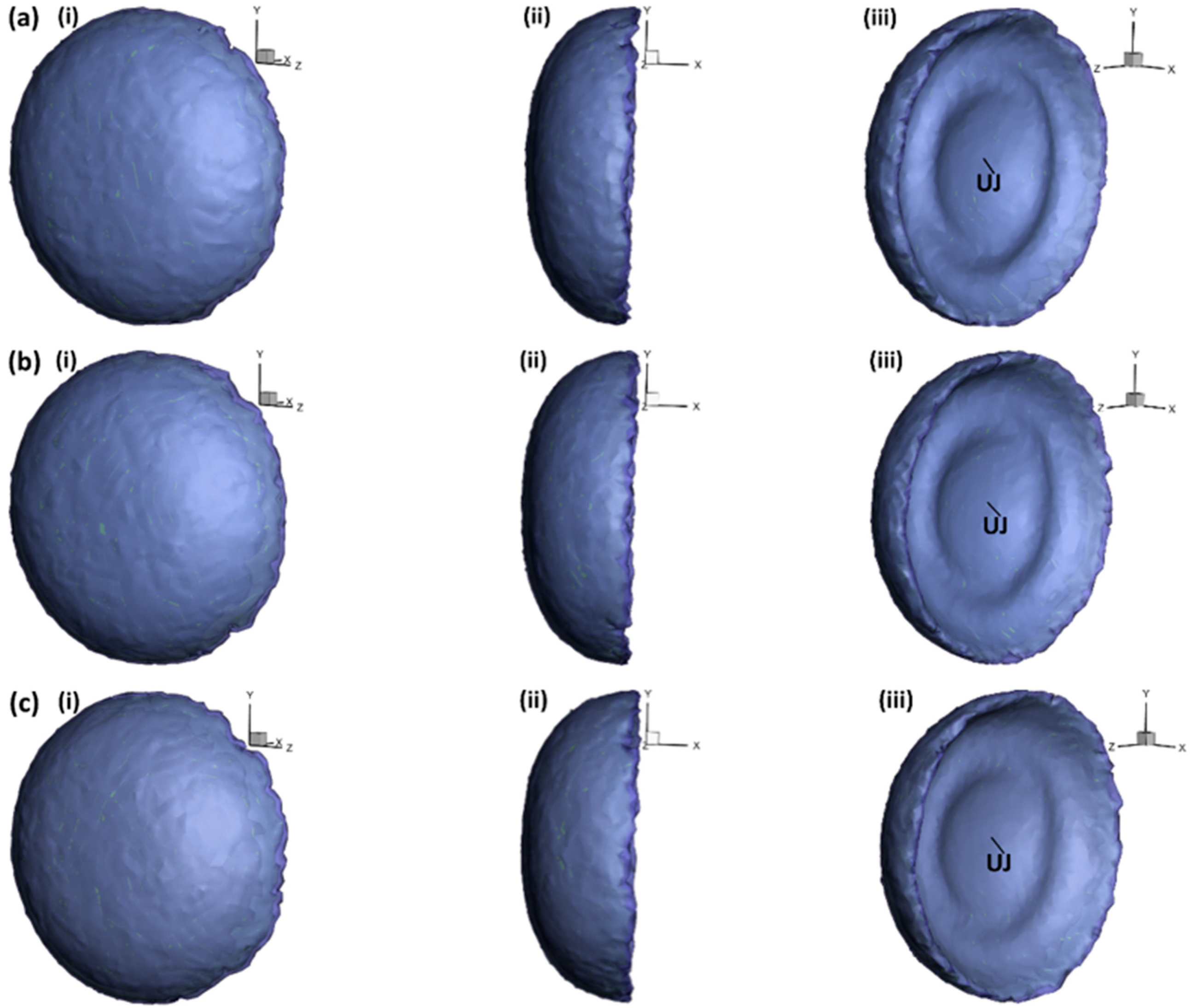
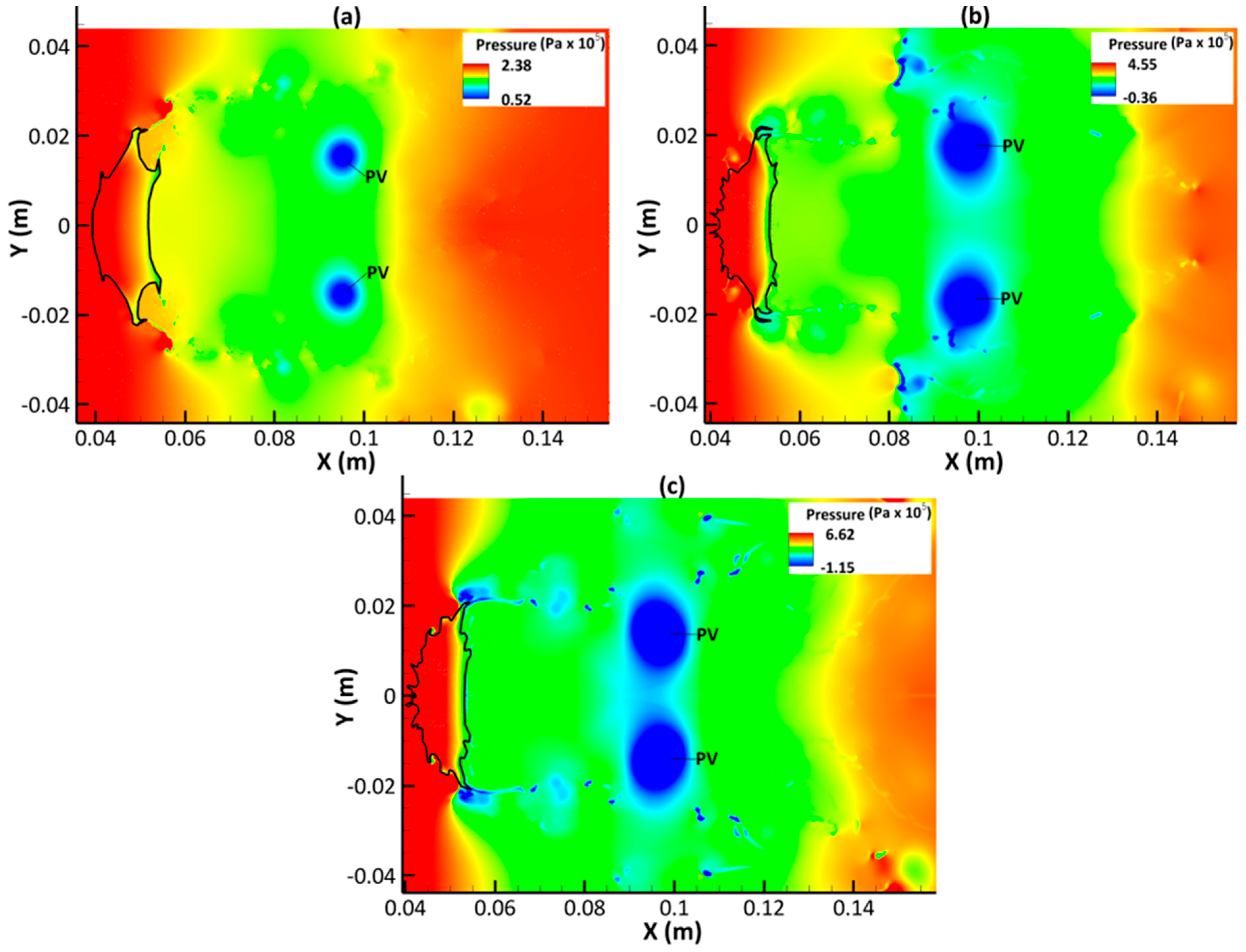
• An upstream jet is formed as a result of the wake recirculation zone caused by the primary vortex pair. This upstream jet impinges on the drop leeward side, promoting the compression and hollowing of the deforming drop.
• The complex flow fields in the wake region are mainly due to the interaction of three vortex systems (primary, secondary, and tertiary) shedding from the deformed drop leeward side periphery. The secondary and tertiary vortices have a relatively short life span, whereas the primary vortices are still clearly observable further downstream towards the end of simulation time.
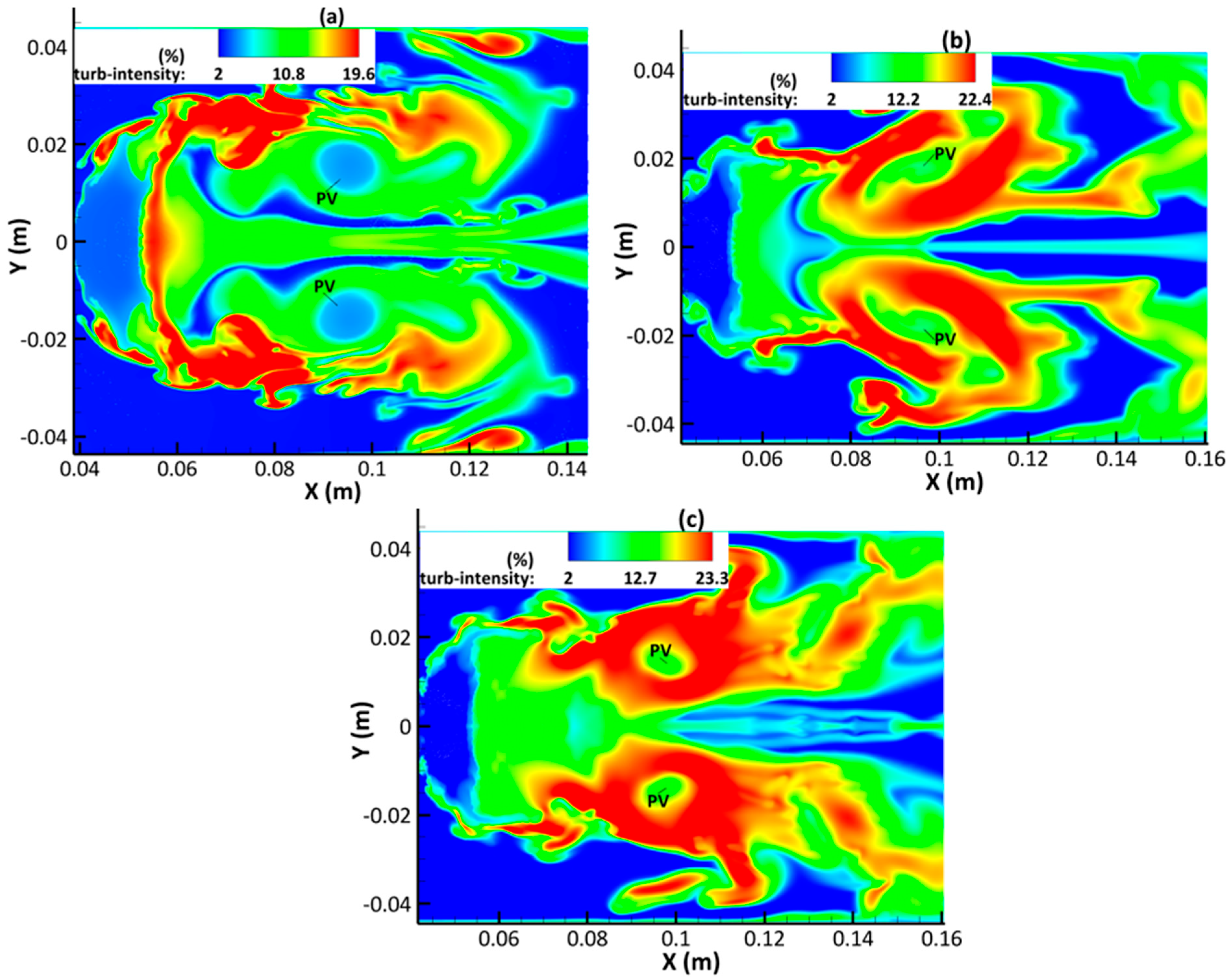
• The wake flow downstream from the severely deformed drop at the late-stage has become fully developed turbulent flow, with the maximum turbulence intensity reaching about 24%.

From our numerical investigation of the effect of Mach number ($Ma$) changes on the SLDI, the following key findings are achieved:

• The liquid sheet propagates faster in the downstream direction as $Ma$ increases. Also, the flattening of the leeward end, i.e., the extent of the flattened region bounded by downstream separation points, contracts as $Ma$ increases because of a reduction of the pressure imposed on the leeward side as well as a reduction in the velocity of the evolving upstream jet.
• Similarly, the stretching of the liquid sheet at the equator is weakened as $Ma$ increases, indicating that the liquid sheet grows less rapidly at higher $Ma$. This is because the evolution of propagative waves induced by Kelvin–Helmholtz instabilities on the surface of the deformed drop are suppressed at higher $Ma$. This suppression is due to the stabilizing effects of compressibility on the flow disturbance at these higher $Ma$.
• With respect to the distribution of shed particles, fluid materials, and micro-drops, this study showed that, as $Ma$ increased, the shed fragments are constrained within a narrower area ahead of the distorted liquid sheet. This is because the stripping points at the equator have folded. As most of the material stripping now take place at these positions, the shed particles and micro-drops have a more confined spread.
• As $Ma$ rises, there is an increase in the amount of small-scale flow structures characterized by high vorticity, such that the turbulent flow in the far-field wake region is fully developed.
• Finally, as $Ma$ increases, the magnitude of turbulent intensity increases around and within the primary vortex, and the maximum value of turbulence intensity also increases across the flow field.

References

1. Kaiser, J.W.J.; Winter, J.M.; Adami, S.; Adams, N.A. Investigation of interface deformation dynamics during high-weber number cylindrical droplet breakup. Int. J. Multiph. Flow 2020, 132, 103409. [Google Scholar] [CrossRef]
2. Lee, C.H.; Reitz, R.D. An experimental study of the effect of gas density on the distortion and breakup mechanism of drops in high speed gas stream. Int. J. Multiph. Flow 2000, 26, 229–244. [Google Scholar] [CrossRef]
3. Lebanoff, A.P.; Dickerson, A.K. Drop impact onto pine needle fibers with non-circular cross section. Phys. Fluids 2020, 32, 092113. [Google Scholar] [CrossRef]
4. Agrawal, M.; Katiyar, R.K.; Karri, B.; Sahu, K.C. Experimental investigation of a nonspherical water droplet falling in air. Phys. Fluids 2020, 32, 112105. [Google Scholar] [CrossRef]
5. Villermaux, E. Fragmentation. Annu. Rev. Fluid Mech. 2007, 39, 419–446. [Google Scholar] [CrossRef]
6. Kumar, A.; Sahu, S. Liquid jet disintegration memory effect on downstream spray fluctuations in a coaxial twin-fluid injector. Phys. Fluids 2020, 32, 073302. [Google Scholar] [CrossRef]
7. Liu, L.H.; Fu, Q.F.; Yang, L.J. Linear stability analysis of liquid jet exposed to subsonic crossflow with heat and mass transfer. Phys. Fluids 2021, 33, 034111. [Google Scholar] [CrossRef]
8. Chou, W.H.; Gamboa, A.; Morales, J.O. Inkjet printing of small molecules, biologics, and nanoparticles. Int. J. Pharm. 2021, 600, 120462. [Google Scholar] [CrossRef] [PubMed]
9. Liu, Y.Y.; Derby, B. Experimental study of the parameters for stable drop-on-demand inkjet performance. Phys. Fluids 2019, 31, 032004. [Google Scholar] [CrossRef]
10. Antonopoulou, E.; Harlen, O.G.; Walkley, M.A.; Kapur, N. Jetting behavior in drop-on-demand printing: Laboratory experiments and numerical simulations. Phys. Rev. Fluids 2020, 5, 043603. [Google Scholar] [CrossRef]
11. Sykes, T.C.; Castrejon-Pita, A.A.; Castrejon-Pita, J.R.; Harbottle, D.; Khatir, Z.; Thompson, H.M.; Wilson, M.C. Surface jets and internal mixing during the coalescence of impacting and sessile droplets. Phys. Rev. Fluids 2020, 5, 023602. [Google Scholar] [CrossRef]
12. Wu, H.; Zhang, F.J.; Zhang, Z.Y. Droplet breakup and coalescence of an internal-mixing twin-fluid spray. Phys. Fluids 2021, 33, 013317. [Google Scholar] [CrossRef]
13. Xu, M.H.; Li, X.R.; Riseman, A.; Frostad, J.M. Quantifying the effect of extensional rheology on the retention of agricultural sprays. Phys. Fluids 2021, 33, 032107. [Google Scholar] [CrossRef]
14. Guildenbecher, D.R.; Lopez-Rivera, C.; Sojka, P.E. Secondary atomization. Exp. Fluids 2009, 46, 371–402. [Google Scholar] [CrossRef]
15. Chen, H. Two-dimensional simulation of stripping breakup of a water droplet. AIAA J. 2008, 46, 1135–1143. [Google Scholar] [CrossRef]
16. Zhu, W.; Zhao, N.; Jia, X.; Chen, X.; Zheng, H. Effect of airflow pressure on the droplet breakup in the shear breakup regime. Phys. Fluids 2021, 33, 053309. [Google Scholar] [CrossRef]
17. Pilch, M.; Erdman, C.A. Use of breakup time data and velocity history data to predict the maximum size of stable fragments for acceleration-induced breakup of a liquid drop. Int. J. Multiph. Flow 1987, 13, 741–757. [Google Scholar] [CrossRef]
18. Hsiang, L.-P.; Faeth, G.M. Drop deformation and breakup due to shock wave and steady disturbances. Int. J. Multiph. Flow 1995, 21, 545–560. [Google Scholar] [CrossRef]
19. Hsiang, L.-P.; Faeth, G.M. Near-limit drop deformation and secondary breakup. Int. J. Multiph. Flow 1992, 18, 635–652. [Google Scholar] [CrossRef]
20. Theofanous, T.G.; Li, G.J.; Dinh, T.N. Aerobreakup in rarefied supersonic gas flows. J. Fluids Eng. 2004, 126, 516–527. [Google Scholar] [CrossRef]
21. Nicholls, J.A.; Ranger, A.A. Aerodynamic shattering of liquid drops. AIAA J. 1969, 7, 285–290. [Google Scholar] [CrossRef]
22. Dai, Z.; Faeth, G.M. Temporal properties of secondary drop breakup in the multimode breakup regime. Int. J. Multiph. Flow 2001, 27, 217–236. [Google Scholar] [CrossRef]
23. Harper, E.Y.; Grube, G.W.; Chang, I.-D. On the breakup of accelerating liquid drops. J. Fluid Mech. 1972, 52, 565–591. [Google Scholar] [CrossRef]
24. Theofanous, T.G. Aerobreakup of Newtonian and viscoelastic liquids. Annu. Rev. Fluid Mech. 2011, 43, 661–690. [Google Scholar] [CrossRef]
25. Wierzba, A.; Takayama, K. Experimental investigation of the aerodynamic breakup of liquid drops. AIAA J. 1988, 26, 1329–1335. [Google Scholar] [CrossRef]
26. Chou, W.H.; Hsiang, L.-P.; Faeth, G.M. Temporal properties of drop breakup in the shear breakup regime. Int. J. Multiph. Flow 1997, 23, 651–669. [Google Scholar] [CrossRef]
27. Igra, D.; Ogawa, T.; Takayama, K. A parametric study of water column deformation resulting from shock wave loading. At. Sprays 2002, 12, 577–591. [Google Scholar] [CrossRef]
28. Liu, Z.; Reitz, R.D. An analysis of the distortion and breakup mechanisms of high speed liquid drops. Int. J. Multiph. Flow 1997, 23, 631–650. [Google Scholar] [CrossRef]
29. Joseph, D.D.; Belanger, J.; Beavers, G.S. Breakup of a liquid drop suddenly exposed to a high-speed airstream. Int. J. Multiph. Flow 1999, 25, 1263–1303. [Google Scholar] [CrossRef]
30. Hirahara, H.; Kawahashi, M. Experimental investigation of viscous effects upon a breakup of droplets in high-speed air flow. Exp. Fluids 1992, 13, 423–428. [Google Scholar] [CrossRef]
31. Theofanous, T.G.; Li, G.J. On the physics of aerobreakup. Phys. Fluids 2008, 20, 052103. [Google Scholar] [CrossRef]
32. Liu, N.; Wang, Z.; Sun, M.; Wang, H.; Wang, B. Numerical simulation of liquid droplet breakup in supersonic flows. Acta Astronaut. 2018, 145, 116–130. [Google Scholar] [CrossRef]
33. Engel, O.G. Fragmentation of water drops in the zone behind an air shock. J. Res. Natl. Bur. Stand. 1958, 60, 245–280. [Google Scholar] [CrossRef]
34. Waldman, G.D.; Reinecke, W. Raindrop breakup in the shock layer of a high-speed vehicle. AIAA J. 1972, 10, 1200–1204. [Google Scholar] [CrossRef]
35. Theofanous, T.G.; Mitkin, T.G.; Ng, C.L.; Chang, C.H.; Deng, X.; Sushchikh, S. The physics of aerobreakup. II. Viscous liquids. Phys. Fluids 2012, 24, 022104. [Google Scholar] [CrossRef]
36. Theofanous, T.G.; Mitkin, T.G.; Ng, C.L. The physics of aerobreakup. III. Viscoelastic liquids. Phys. Fluids 2013, 25, 032101. [Google Scholar] [CrossRef]
37. Gonor, A.L.; Zolotova, N.V. Spreading and break-up of a drop in a gas stream. Acta Astronaut. 1984, 11, 137–142. [Google Scholar] [CrossRef]
38. Khosla, S.; Smith, C.E.; Throckmorton, R.P. Detailed understanding of drop atomization by gas crossflow using the volume of fluid method. In Proceedings of the Nineteenth Annual Conference on Liquid Atomization and Spray Systems, Toronto, ON, Canada, 23–26 May 2006; ILASS-Americas: Toronto, ON, Canada, 2006. [Google Scholar]
39. Yang, W.; Jia, M.; Che, Z.; Sun, K.; Wang, T. Transitions of deformation to bag breakup and bag to bag-stamen breakup for droplets subjected to a continuous gas flow. Inter. J. Heat Mass Transf. 2017, 111, 884–894. [Google Scholar] [CrossRef]
40. Meng, J.C.; Colonius, T. Numerical simulation of the aerobreakup of a water droplet. J. Fluid Mech. 2018, 835, 1108–1135. [Google Scholar] [CrossRef]
41. Aslani, M.; Regele, J.D. A localized artificial diffusivity method to simulate compressible multiphase flows using the stiffened gas equation of state. Int. J. Numer. Meth. Fluids 2018, 88, 413–433. [Google Scholar] [CrossRef]
42. Igra, D.; Takayama, K. A Study of Shock Wave Loading on a Cylindrical Water Column; Technical Report; Institute of Fluid Science, Tohoku University: Sendai, Japan, 2001. [Google Scholar]
43. Meng, J.C.; Colonius, T. Numerical simulations of the early stages of high-speed droplet breakup. Shock Waves 2014, 25, 399–414. [Google Scholar] [CrossRef]
44. ANSYS Academic Research, ANSYS Fluent Theory Guide; ANSYS Help System; ANSYS, Inc.: Southpointe/Canonsburg, PA, USA, 2020.
45. Hinze, J.O. Turbulent Flow Regions with Shear Stress and Mean Velocity Gradient of Opposite Sign. Appl. Sci. Res. 1970, 22, 163–175. [Google Scholar] [CrossRef]
46. Onwuegbu, S.; Yang, Z. Numerical analysis of shock interaction with a spherical bubble. AIP Adv. 2022, 12, 025215. [Google Scholar] [CrossRef]
47. Onwuegbu, S.; Yang, Z.; Xie, J. Numerical simulation of the interaction between a planar shock wave and a cylindrical bubble. Modelling 2024, 5, 483–501. [Google Scholar] [CrossRef]
48. Launder, B.E.; Reece, G.J.; Rodi, W. Progress in the Development of a Reynolds-Stress Turbulence Closure. J. Fluid Mech. 1975, 68, 537–566. [Google Scholar] [CrossRef]
49. Gibson, M.M.; Launder, B.E. Ground Effects on Pressure Fluctuations in the Atmospheric Boundary Layer. J. Fluid Mech. 1978, 86, 491–511. [Google Scholar] [CrossRef]
50. Launder, B.E. Second-Moment Closure: Present... and Future? Int. J. Heat Fluid Flow 1989, 10, 282–300. [Google Scholar] [CrossRef]
51. Daly, B.J.; Harlow, F.H. Transport Equations in Turbulence. Phys. Fluids 1970, 13, 2634–2649. [Google Scholar] [CrossRef]
52. Lien, F.S.; Leschziner, M.A. Assessment of Turbulent Transport Models Including Non-Linear RNG Eddy-Viscosity Formulation and Second-Moment Closure. Comput. Fluids 1994, 23, 983–1004. [Google Scholar] [CrossRef]
53. Shyue, K.M. An efficient shock-capturing algorithm for compressible multicomponent problems. J. Comput. Phys. 1998, 142, 208–242. [Google Scholar] [CrossRef]
54. Onwuegbu, S.; Yang, Z.; Xie, J. Numerical study of the shear stripping of a liquid drop under shock wave loading. Chin. J. Aeronaut. 2025; submitted. [Google Scholar]
55. Serthian, J.A.; Smereka, P. Level set methods for fluid interfaces. Ann. Rev. Fluid Mech. 2003, 35, 341–372. [Google Scholar] [CrossRef]
56. Olsson, E.; Kreiss, G.; Zahedi, S. A Conservative Level Set Method for Two Phase Flow II. J. Comput. Phys. 2007, 225, 785–807. [Google Scholar] [CrossRef]
57. Jofre, L.; Lehmkuhl, O.; Castro, J.; Oliva, A. A 3-D volume-of-fluid advection method based on cell-vertex velocities. Comput. Fluids 2014, 94, 14–29. [Google Scholar] [CrossRef]
58. Balcazar, N.; Lehmkuhl, O.; Jofre, L.; Rigola, J.; Olivia, A. A coupled volume-of-fluid/level-set method for simulation of two-phase flows on unstructured meshes. Comput. Fluids 2016, 124, 12–29. [Google Scholar] [CrossRef]
59. Coralic, V.; Colonius, T. Finite-volume WENO scheme for viscous compressible multicomponent flows. J. Comput. Phys. 2014, 274, 95–121. [Google Scholar] [CrossRef] [PubMed]
60. Ansari, M.R.; Azadi, R.; Salimi, E. Capturing of interface topological changes in two-phase gas-liquid flows using a coupled volume-of-fluid and level-set method (VOSET). Comput. Fluids 2016, 125, 82–100. [Google Scholar] [CrossRef]
61. Sussman, M.; Fatemi, E.; Smereka, P.; Osher, S. An improved level set method for incompressible two-phase flows. Comput. Fluids 1998, 27, 663–680. [Google Scholar] [CrossRef]
62. Luo, K.; Shao, C.; Yang, Y.; Fan, J. A mass conserving level set method for detailed numerical simulation of liquid atomization. J. Comput. Phys. 2015, 298, 495–519. [Google Scholar] [CrossRef]
63. Wang, Z.; Li, S.; Chen, R.; Xun, Z.; Liao, Q.; Ye, D.; Zhang, B. Numerical study on dynamic behaviors of the coalescence between the advancing liquid meniscus and multi-droplets in a microchannel using CLSVOF method. Comput. Fluids 2018, 170, 341–348. [Google Scholar] [CrossRef]
64. Cash, J.R.; Karp, A.H. A variable order Runge-Kutta method for initial value problems with rapidly varying right-hand sides. ACM Trans. Math. Software 1990, 16, 201–222. [Google Scholar] [CrossRef]
65. Reitz, R.D. Mechanisms of atomization processes in high-pressure vaporizing sprays. At. Spray Technol. 1987, 3, 309–337. [Google Scholar]
66. Liu, A.B.; Mather, D.; Reitz, R.D. Modeling the effects of drop drag and breakup on fuel sprays. J. Engines. 1993, 102, 83–95. [Google Scholar]
67. Van Leer, B. Toward the Ultimate Conservative Difference Scheme. V. A Second Order Sequel to Godunov’s Method. J. Comput. Phys. 1979, 32, 101–136. [Google Scholar] [CrossRef]
68. Sembian, S.; Liverts, M.; Tillmark, N.; Apazadis, N. Plane shock wave interaction with a cylindrical column. Phys. Fluids 2016, 28, 056102. [Google Scholar] [CrossRef]
69. Houghton, E.L.; Brock, A.E. Table IV: Flow of dry air through a plane normal shock wave. In Tables for the Compressible Flow of Dry Air, 3rd ed.; Arnold, E., Ed.; Athenaeum Press Ltd.: Newcastle upon Tyne, UK, 1993; Volume 3, pp. 40–46. [Google Scholar]
70. Hillier, R. Computation of shock wave diffraction at a ninety degrees convex edge. Shock Waves 1991, 1, 89–98. [Google Scholar] [CrossRef]
71. Ingram, D.M.; Causon, D.M.; Mingham, C.G. Developments in Cartesian cut cell methods. Math. Comput. Simul. 2013, 61, 561–572. [Google Scholar] [CrossRef]
72. Berger, M.; Aftosmis, M.J.; Allmaras, S.R. Progress towards a cartesian cut-cell methods for viscous compressible flow. In Proceedings of the 50th AIAA Aerospace Sciences Meeting Including the New Horizons Forum and Aerospace Exposition, Nashville, TN, USA, 9–12 January 2012; American Institute of Aeronautics and Astronautics: Nashville, TN, USA, 2012. [Google Scholar]
73. Johnson, M.W. A novel Cartesian CFD cut cell approach. Comput. Fluids 2013, 79, 105–119. [Google Scholar] [CrossRef]
74. Holleman, R.; Fringer, O.; Stacey, M. Numerical diffusion for flow-aligned unstructured grids with application to estuarine modelling. Int. J. Numer. Methods Fluids 2013, 72, 1117–1145. [Google Scholar] [CrossRef]
75. Zubair, M.; Abdullah, M.Z.; Ahmad, K.A. Hybrid mesh for nasal airflow studies. Comput. Math. Methods Med. 2013, 1, 727362. [Google Scholar] [CrossRef] [PubMed]
76. Lawlor, O.; Chakravorty, S.; Wilmarth, T.; Choudhury, N.; Dooley, I. Parfum: A parallel framework for unstructured meshes for scalable dynamic physics applications. Eng. Comput. 2006, 22, 215–235. [Google Scholar] [CrossRef]
77. Jahangirian, A.; Shoraka, Y. Adaptive unstructured grid generation for engineering computation of aerodynamic flows. Math. Comput. Simulat. 2008, 78, 627–644. [Google Scholar] [CrossRef]
78. Cant, R.S.; Ahmed, U.; Fang, J.; Chakarborty, N.; Nivarti, G.; Moulinec, C.; Emerson, D.R. An unstructured adaptive mesh refinement approach for computational fluid dynamics of reacting flows. J. Comput. Phys. 2022, 468, 111480. [Google Scholar] [CrossRef]
79. Wang, Y.; Dong, G. A numerical study of shock-interface interaction and prediction of the mixing zone growth in inhomogeneous medium. Acta Mech. Sin. 2022, 38, 122163. [Google Scholar] [CrossRef]
80. Yu, B.; Li, L.; Xu, H.; Zhang, B.; Liu, H. Effects of Reynolds number and Schmidt number on variable density mixing in shock bubble interaction. Acta Mech. Sin. 2022, 38, 121256. [Google Scholar] [CrossRef]
81. Karyagin, V.P.; Lopatkin, A.I.; Shvets, A.I.; Shilin, N.M. Experimental investigation of the separation of flow around a sphere. Fluid Dyn. 1991, 26, 126–129. [Google Scholar] [CrossRef]
82. Nagata, T.; Nonomura, T.; Takahashi, S.; Mizuno, Y.; Fukuda, K. Investigation on subsonic to supersonic flow around a sphere at low Reynolds number of between 50 and 300 by direct numerical simulation. Phys. Fluids 2016, 28, 056101. [Google Scholar] [CrossRef]
83. Papamoschou, D.; Roshko, A. The compressible turbulent shear layer: An experimental study. J. Fluid Mech. 1988, 197, 453–477. [Google Scholar] [CrossRef]
84. Jalaal, M.; Mehravaran, K. Transient growth of droplet instabilities in a stream. Phys. Fluids 2014, 26, 012101. [Google Scholar] [CrossRef]
85. Wang, Z.; Hopfes, T.; Giglmaier, M.; Adams, N.K. Effect of Mach number on droplet aerobreakup in shear stripping regime. Exp. Fluids 2020, 61, 193. [Google Scholar] [CrossRef] [PubMed]
Figure 1. Computational domain plus the initial and boundary conditions.
Aerospace 12 00648 g001
Figure 2. (a) Computational mesh and (b) close view of fine mesh around drop from AMR.
Aerospace 12 00648 g002
Figure 3. Comparison of numerical results from different turbulence models against experimental data (Igra et al., [27]) from the compression phase. Reprinted/adapted with permission from Ref. [27]. Copyright 2024, Elsevier.
Aerospace 12 00648 g003
Figure 4. Variations of the normalized width of the deformed drop against dimensionless time,  T , compared to experimental data (Igra et al., [27]).
Aerospace 12 00648 g004
Figure 5. Variations of the normalized height of the deformed drop against dimensionless time,  T , compared to experimental data (Igra et al., [27]).
Aerospace 12 00648 g005
Figure 6. Evolution of the normalized drop area against dimensionless time,  T , compared to experimental data (Igra et al., [27]).
Aerospace 12 00648 g006
Figure 7. Snapshots of (i) volume fraction contours on the central  x y  plane and (ii) iso-surfaces of volume fraction at: (a T = 0.37 ; (b T = 0.45 ; (c T = 0.53 ; (d T = 0.60 ; (e T = 0.64 ; (f T = 0.68 .
Aerospace 12 00648 g007
Figure 8. Snapshots of vorticity contours on the central  x y  plane at: (a T = 0.37 ; (b T = 0.45 ; (c T = 0.53 ; (d T = 0.60 ; (e T = 0.64 ; (f T = 0.68 .
Aerospace 12 00648 g008
Figure 9. Visualization of the drop disintegration process at: (a T = 0.60 ; (b T = 0.64 ; (c T = 0.68 .
Aerospace 12 00648 g009
Figure 10. Snapshots of the streamlines on the central  x y  plane at: (a T = 0.37 ; (b T = 0.45 ; (c T = 0.53 ; (d T = 0.60 ; (e T = 0.64 ; (f T = 0.68 .
Aerospace 12 00648 g010
Figure 11. Contours of velocity magnitude on the central  x y  plane during the compression and late-time stages of the water disintegration process at: (a T = 0.37 ; (b T = 0.45 ; (c T = 0.53 ; (d T = 0.60 ; (e T = 0.64 ; and (f T = 0.68 .
Aerospace 12 00648 g011
Figure 12. Contours of turbulence intensity on the central  x y  plane during the compression and late-time stages of the water disintegration process at: (a T = 0.37 ; (b T = 0.45 ; (c T = 0.53 ; (d T = 0.60 ; (e T = 0.64 ; (f T = 0.68 .
Aerospace 12 00648 g012
Figure 13. Dimensionless drift against dimensionless time,  T , for  M a = 1.47 M a = 2.0 , and  M a = 2.4 . Dimensionless drift against dimensionless time for  M a = 1.47  has been compared to experimental data (Igra et al., [27]).
Aerospace 12 00648 g013
Figure 14. Snapshots of volume fraction contours on the central  x y  plane at  T = 0.45  for: (a M a = 1.47 ; (b M a = 2.0 ; and (c M a = 2.4 .
Aerospace 12 00648 g014
Figure 15. Snapshots of vorticity contours on the central  x y  plane at  T = 0.45  for: (a M a = 1.47 ; (b M a = 2.0 ; and (c M a = 2.4 .
Aerospace 12 00648 g015
Figure 16. Representation of the vortex systems on the central  x y  plane using streamlines at  T = 0.45  for: (a M a = 1.47 ; (b M a = 2.0 ; and (c M a = 2.4 .
Aerospace 12 00648 g016
Figure 17. Contours of velocity magnitude on the central  x y  plane at  T = 0.45  for: (a M a = 1.47 ; (b M a = 2.0 ; and (c M a = 2.4 .
Aerospace 12 00648 g017
Figure 18. Contours of pressure on the central  x y  plane at  T = 0.45  for: (a M a = 1.47 ; (b M a = 2.0 ; and (c M a = 2.4 .
Aerospace 12 00648 g018
Figure 19. Contours of turbulence intensity on the central  x y  plane at  T = 0.45  for: (a M a = 1.47 ; (b M a = 2.0 ; and (c M a = 2.4 .
Aerospace 12 00648 g019