A Comparative Study of Unsupervised Deep Learning Methods for Anomaly Detection in Flight Data

Abstract

This paper provides a comparative study of unsupervised Deep Learning (DL) methods for anomaly detection in Flight Data Monitoring (FDM). The paper applies Long Short-Term Memory (LSTM), Gated Recurrent Units (GRUs), Convolutional Neural Network (CNN), classic Transformer architecture, and LSTM combined with a self-attention mechanism to real-world flight data and compares the results to the current state-of-the-art flight data analysis techniques applied in the industry. The paper finds that LSTM, when integrated with a self-attention mechanism, offers notable benefits over other deep learning methods as it effectively handles lengthy time series like those present in flight data, establishes a generalized model applicable across various airports and facilitates the detection of trends across the entire fleet. The results were validated by industrial experts. The paper additionally investigates a range of methods for feeding flight data (lengthy time series) to a neural network. The innovation of this paper involves utilizing Transformer architecture and LSTM with self-attention mechanism for the first time in the realm of aviation data, exploring the optimal method for inputting flight data into a model and evaluating all deep learning techniques for anomaly detection against the ground truth determined by human experts. The paper puts forth a compelling case for shifting from the existing method, which relies on examining events through threshold exceedances, to a deep learning-based approach that offers a more proactive style of data analysis. This not only enhances the generalization of the FDM process but also has the potential to improve air transport safety and optimize aviation operations.

1. Introduction

This paper is a comparative analysis of unsupervised deep learning methods for anomaly detection in real-world flight data. Flight Data Monitoring (FDM) is generally defined as a proactive and non-punitive use of digital flight data from routine operations to improve aviation safety conducted by airlines as a means of improving the safety and operation of their aircraft fleet. Modern civil aircraft are required to have flight data recorders with a minimum ability to store 88 flight parameters for 25 hours [1]. This data is typically downloaded from the aircraft and analyzed offline through statistical methods to highlight exceedances of such parameters. Such occurrences are then investigated by the airline’s safety officers with the aim of improving safety, through implementing standard operating procedures and promoting good airmanship. However, with progress in data storage technology, aircraft manufacturers have taken the opportunity to record more data which is then fed into safety and improvement of their product. For example, the Boeing 787 can record approximately 2000 flight parameters in 50 hours. This makes data analysis laborious.

Despite that the introduction of FDM has improved aviation safety substantially, this suffers from a number of limitations, namely:

• The current occurrence-based system relies on the human operator to establish patterns in exceedances from a particular aircraft or the fleet. It can be an overwhelming exercise for a human operator.
• Such occurrences are identified through set thresholds based on past experience, including incidents or accidents. As a result, the system cannot detect internal vulnerabilities or explore unknown safety issues. For examples, Boeing 737 Max aircraft’s software issues resulting in plane’s nose being pushed down unexpectedly and pilots struggled to regain control.
• Traditional Machine Learning (ML)-based techniques are dependent on quality of flight data, airports, type of aircraft and other various input factors as shown in the scholarly work [2]. The various input factors must be adjusted accordingly, but methods based on deep learning are capable of producing generalized models.

As suggested by [3] redefining incidents and thresholds may address these limitations. However, this will still maintain the limitation of being incapable of foreseeing future problems that may cause incidents. Therefore, while the data recording aspect has improved dramatically, the data analysis aspect has been lagging. Traditional ML techniques can aid in revealing these unique flight patterns; however, their reliance on various input factors such as the number of flights, the airports involved and so forth hinders the generalization of the Flight Data Monitoring (FDM) process. Consequently, it may not be possible to develop a generalized model for FDM. Therefore, there is a need for a deep learning-based generalized model that can identify anomalies within flight data. Additionally, deep learning excels at extracting temporal features (identifying and representing flight parameters recorded at certain intervals) and offers an end-to-end learning approach, which means that only minimal pre-processing of the flight data parameters is necessary. Deep learning (DL) is a branch of machine learning that mimics the cognitive functions of human brain to interpret data. This approach involves the utilization of artificial neural networks made up of several layers (hence termed “deep”) to detect patterns and predict results. DL models are formed with interconnected layers of artificial neurons, commonly known as neural networks. Each layer adeptly processes the data it receives and subsequently passes it on to the subsequent layer. As the data moves through multiple layers, the model becomes capable of recognizing more complex patterns and relationships. For effective learning, DL necessitates a large volume of data, making its reliance on data a considerable limitation in this domain. Anomaly detection encompasses the identification of patterns within data that deviate from expected behavior [4]. Numerous algorithms and approaches for anomaly identification exist and an extensive literature review has been carried out by [4,5,6].

In a general context, DL techniques for anomaly detection can be categorized as either supervised or unsupervised, depending on how flight data is processed. Supervised approaches utilize a labeled dataset to aid in the training of the models. These models, which are trained solely on normal data, are capable of identifying unusual data that they have not previously encountered. The task of annotating (labeling) data is both time-consuming and expensive. It requires the participation of human experts, thus making it prone to human biases. In addition, datasets that contain anomalies may lead to a tendency to skew the data, as normal data is often in much greater abundance than anomalous data. On the other hand, unsupervised techniques allow learning algorithms to reveal concealed patterns in datasets that lack labels. Unlabeled data pertains to information that is not classified as either normal or anomalous. In anomaly detection, the goal is to recognize instances that deviate from the normal data pattern. When applying these methodologies in the aviation industry, the detection or formulation of cases based on specific anomalies heavily depends on human knowledge. It is impractical to acquire every instance of unusual flights (outliers); therefore, it is essential to select the right examples for labeling to guarantee accurate classification with the least number of labels. This is known as the problem of label acquisition [7]. The challenge of detecting anomalies presented in this paper cannot be effectively tackled using supervised methods, as the main goal is to uncover anomalies without any previous understanding of what is deemed “normal” or “abnormal.” Consequently, unsupervised anomaly detection methods provide significant advantages in the realm of FDM, as they help in modeling the underlying structure or distribution within the data, facilitating a more profound comprehension of the data without dependence on labels.

Furthermore, unsupervised anomaly detection techniques can be divided into traditional machine learning methods like clustering or modern deep learning techniques such as Recurrent Neural Networks (RNNs) that employ multiple layers of neurons. The identification of anomalies in flight data through traditional ML depends on factors including the destination airport and the number of flights being examined. When these factors are taken into account, they introduce a considerable amount of variability in the analysis results. Modifying any of these factors results in a corresponding change in the outcomes. Therefore, a more comprehensive approach is pursued through the application of deep learning methodologies. By utilizing deep neural networks, a data-oriented model can be developed to generalize the anomaly detection process in flight data. This model is established through training on normal flight occurrences drawn from historical flight records. For deep learning techniques to preserve the model’s accuracy, it is essential to label the data so that the model is exclusively trained on normal flights. This paper employs previously validated hybrid-Local Outlier Factor (LOF) technique [2] to label normal and anomalous flights, with the normal flights being utilized to train various DL models. Figure 1 depicts the categorization of flight data as either normal or anomalous flights using hybrid-LOF. The deep learning model is trained using a dataset composed of normal flight records.

2. Literature Review of Unsupervised Deep Learning Techniques

With the advancements in computational resources as well as the proliferation of extensive datasets over time, an increasing number of anomaly detection methodologies for flight data have been introduced, predominantly utilizing deep learning techniques or deep neural networks. Several noteworthy contributions are examined in the succeeding paragraphs.

The Self-Organizing Map Neural Network (SOM NN) utilized by [8] for the identification of anomalies in flight data is characterized as an unsupervised, bifurcated neural network comprising input and output layers. The input layer is composed of vectors of data that require delineation, while the output layer signifies the structured representation of the data. The SOM facilitates the transformation of data points that initially exist in a high-dimensional space into a two-dimensional representation. This facilitates a more comprehensive examination and the organization of the dataset becomes apparent. The Self-Organizing Map Neural Network (SOM NN) identified 8800 anomalous data points across 69 flights. Despite the efficacy of this methodology in pinpointing individual anomalies, it proved insufficient for application as a generalized model or for generating supplementary insights pertaining to anomalies. Recurrent Neural Networks (RNNs), as employed by [9], enable the transmission of hidden layer neuron outputs to other neurons as input, thus permitting the incorporation of prior data, a characteristic that is especially beneficial in the examination of sequential datasets such as historical flight records. Their adaptation of the traditional Recurrent Neural Network (RNN) architecture incorporated the integration of Long Short-Term Memory (LSTM) units alongside Gated Recurrent Units (GRU). This assertion claims that RNNs utilizing LSTM and GRU circumvent the limitations associated with ClusterAD (clustering technique) owing to their proficiency in adeptly handling multivariate sequential data without necessitating any alterations [10]. Thus, it may prove to be optimal for the analysis of flight data. In this study, a dataset encompassing 500 flights was subjected to rigorous analysis. Anomalies were systematically integrated into the simulated dataset, and the effectiveness of anomaly detection mechanisms employing Long Short-Term Memory (LSTM) and Gated Recurrent Unit (GRU) architectures was evaluated, indicating that both LSTM and GRU exhibited enhanced performance in comparison to conventional clustering methodologies. In the scholarly work presented in [11], deep Autoencoders (DAE) are employed on raw time series data collected from a multitude of sensors installed on the aircraft to develop a robust model for identifying anomalies within flight data. The methodology for anomaly detection evaluates the reconstruction error of a DAE that has undergone training on normal (standard) data scenarios. The analysis of the reconstruction error associated with each sensor is undertaken to enhance the process of detection of anomaly. The proposed framework does not require any manually crafted features and functions directly on unprocessed time series data. The model demonstrated shortcomings in the temporal dimension and the training procedure for the model was found to be computationally intensive. The Convolutional Variational Auto-Encoder (CVAE) formulated by [12] represents an unsupervised deep generative framework designed for the identification of anomalies in high-dimensional time-series datasets. The performance of CVAE exceeds that of both traditional and deep learning-based methodologies in the detection of anomalies within aviation data, despite its reliance on data labels to differentiate between normative and anomalous flight instances. This paper implements Convolutional Neural Network (CNN) based autoencoders to detect anomalies. The LSTM-based autoencoders developed by [13] exhibit similarities to the LSTM autoencoders described in this paper. Nonetheless, the model referenced in [13] is exclusively designed for a singular arrival airport (Najaf International Airport) and accounts for merely five flight parameters. A temporal-feature attention mechanism is employed by [14] to construct a deep hybrid model aimed at the detection of flight anomalies. This hybrid model integrates a convolutional autoencoder based on a temporal-feature attention framework with the Hierarchical Density-Based Spatial Clustering of Applications with Noise (HDBSCAN) clustering algorithm [15]. Within this paradigm, the autoencoder is meticulously designed and optimized to capture flight characteristics, while the HDBSCAN serves the function of the anomaly detection module. Given that the autoencoder was solely utilized for the purpose of capturing flight characteristics, the performance of the model was commensurate with that of traditional HDBSCAN models. The deep learning methodology grounded in deep neural networks, as articulated by [16], was employed for the identification and forecasting of potentially destabilized arrival flights at Taipei Songshan Airport. Although the methodology exhibited a commendable degree of precision, its applicability was confined exclusively to unstable approaches and was restricted to a singular airport.

The literature review has uncovered a lack of any research that both applies and compares prominent deep learning (DL) methods. Moreover, a substantial proportion of the current investigations predominantly concentrate on simulated datasets, in stark contrast to this paper, which employs real-world flight data. Furthermore, the DL frameworks established in previous studies demonstrate a lack of generalizability across a range of airport environments. Considering that the realm of DL is still developing, the aviation industry presents considerable opportunities for harnessing its potential. This research intends to present the most recent innovations in DL within the Flight Data Monitoring (FDM) sector.

3. Applications of Deep Learning Techniques

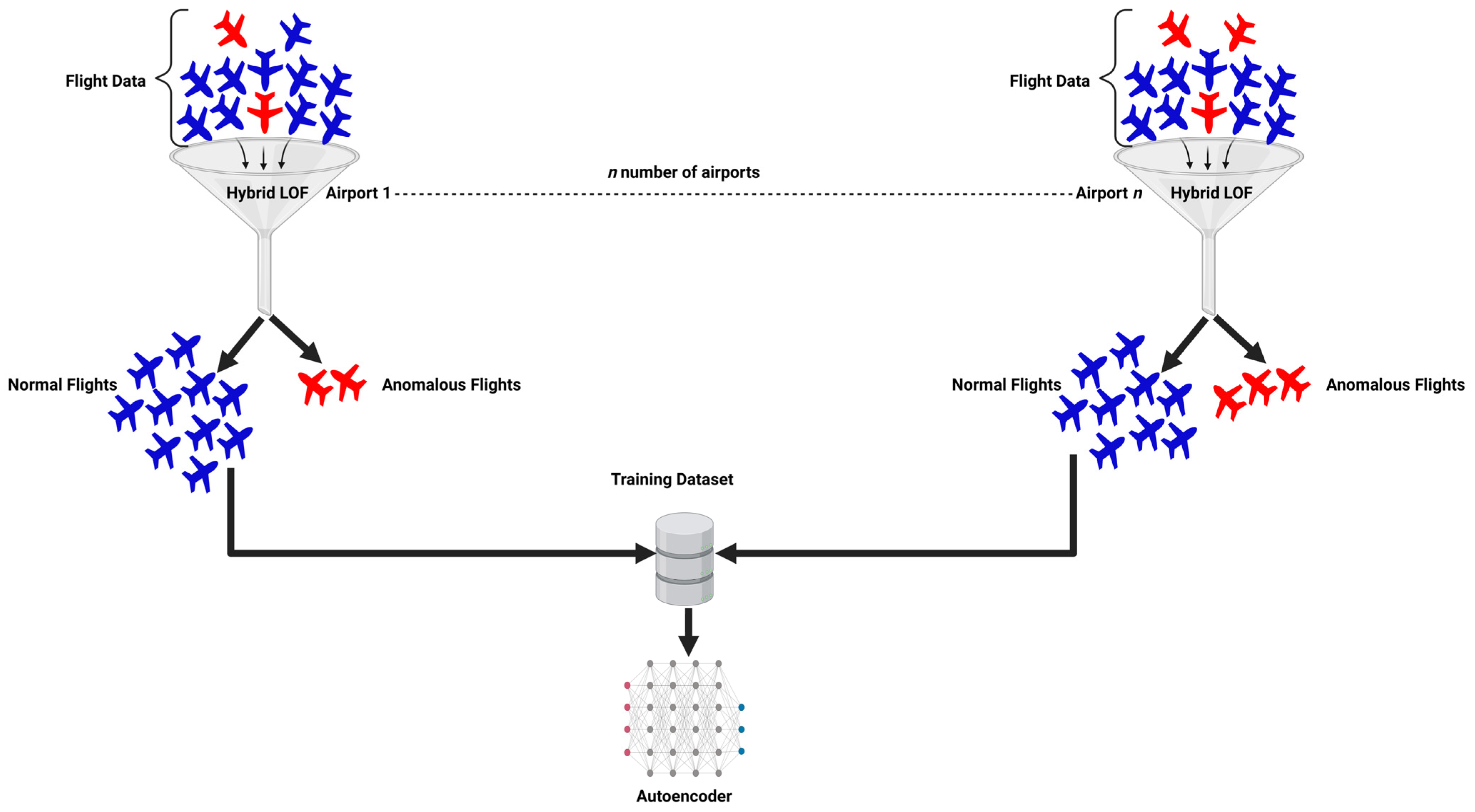
This section applies DL based techniques to a real-world flight dataset. The subsequent subsections provide a detailed explanation of the procedures involved in implementing each technique, emphasizing the significant distinctions in the execution of each method.

3.1. Flight Dataset

The availability of real-world flight data is significantly impeded by the sensitive nature inherent in airline operations and the imperative for pilot personal data protection. In the year 2012, the National Aeronautics and Space Administration (NASA) disseminated a comprehensive database comprising multivariate time series flight data into the public domain [17]. This database, which encompasses a total of 250 GB, pertains to approximately 170,000 flights that occurred in the years spanning from 2001 to 2003 and again in 2010. A cumulative total of 35 tail numbers were meticulously documented as aircrafts traversed between 90 airports situated across the United States of America. Each individual flight is characterized by 186 distinct flight parameters, with sampling frequencies oscillating between 1 Hz and 16 Hz. In order to protect the identities of the airlines and flight crew members, the flight data has been rigorously de-identified.

3.2. Selecting Approach and Landing Phase as a Case Study

In order to define the boundaries of this comparative analysis, the investigation was confined to the approach and landing phase of the flight, as this phase represents the most critical phase of a flight. Over the preceding two decades, it has been observed that more than fifty percent of all fatal and non-fatal incidents culminating in the destruction of an aircraft’s hull occurred during the approach and landing phase, notwithstanding the fact that this specific phase constitutes merely approximately four percent of the overall flight duration [18,19]. Thus, for the analytical purposes, the concluding three minutes of flight duration, which encompasses the approach and landing phase are taken into consideration. A considerable number of flights become unstable during this phase. Conventionally, a stable approach is characterized by a predetermined set of criteria, which are outlined in

Table 1. Rules for a Stabilized Approach.

Approach Rule	Flight Parameter	Unit	Optimal Value for Stabilized Approach
Established on the glide path	Glideslope Deviation	degree	3
Proper air speed	Indicated Airspeed	knots	>VRef & <VRef + 20 knots
Stable descent rate	Inertial Vertical Velocity	feet/minute	750–100 feet/min
Stable engine power setting	Engine 1 to Engine 4 Speed (N1 & N2)	%	30–100%
Flaps configuration	Flap Position	degrees/counts	0–45°
Landing Gear Configuration	Landing gear toggle switch	up/down	down

. In the table the expression “>V_Ref & <V_Ref + 20 knots” means an airspeed greater than the reference landing speed (V_Ref) but less than or equal to V_Ref plus 20 knots. This speed range is often used during the final approach and landing of an aircraft, with V_Ref serving as a baseline and the +20 knots representing a common maximum speed additive for wind and other corrections. When the data pertaining to the aircraft indicate that at least one of these criteria has been violated (evidenced by an exceedance in the flight parameter data), the approach is deemed unstable, prompting a subsequent investigation into the flight. The comparative analysis using DL techniques was executed on three tail number (Tail 652, 653 and 654), which included a total of 2500 flights. These flights culminated in landings at Detroit Metropolitan Wayne County Airport (DTW), Minneapolis–Saint Paul International Airport (MSP), and Memphis International Airport (MEM) within the United States of America.

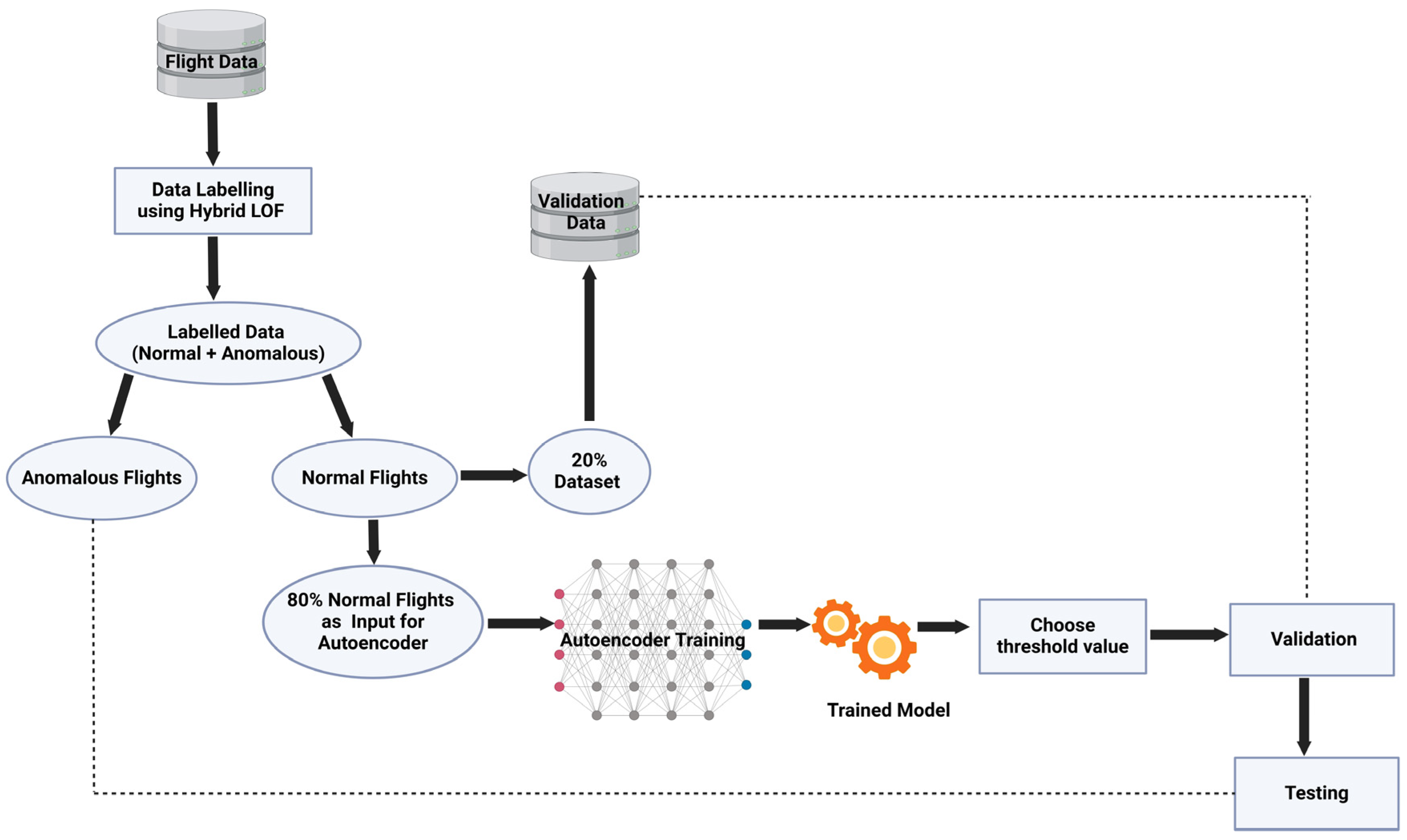
3.3. Data Pre-Processing

The dataset, which was preserved in MAT files (a binary file format used by MATLAB), underwent a procedural transformation to be represented in the structure of Structured Query Language (SQL) tables. This conversion enabled the effective retrieval and application of the data. For each distinct flight, a collection of 132 flight parameters, considered imperative by industry experts, were evaluated. The intentional exclusion of dynamic weather-related parameters guarantees that all flights are subjected to a uniform analysis related to aircraft behavior. As such changes in weather do not lead to anomalies. However, any weather-related occurrences, such as variations in wind speed or direction that affect aircraft behavior and the conduct of the flight crew, are considered based on recordings of other flight parameters like Localizer deviation and alterations in Drift angle caused by shifts in wind direction and speed. This has been thoroughly demonstrated in a case study provided in the work [20]. Specific flight parameters that possess constant values, such as the engine number, were also excluded from the analytical process. The values corresponding to all 132 flight indicators were normalized, given that each flight parameter exhibited a unique spectrum of values and measurement units. The dataset underwent a comprehensive review to detect and amend any instances of missing data or corrupt values. The aforementioned flight parameters were sampled at frequencies varying from 1 hertz to 16 hertz. To ensure the alignment of data points, all flight parameters underwent conversion to a uniform sampling frequency of 16 hertz through the interpolation of values obtained from parameters sampled at lower frequencies. For the purposes of analysis, the concluding three minutes of the flight duration, encompassing the approach and landing phase, were selected. The precise coordinates at which each aircraft made contact with the runway were established by considering a range of flight parameters, including the Flight Phase (PH), the presence of Weight on Wheels (WOW), in addition to the Latitude (LAT) and Longitude (LONG) coordinates. The latitude and longitude coordinates were employed to accurately identify the specific runway utilized during landing. Moreover, all flight trajectories were adjusted to correspond to the designated altitude of the airport, thereby eliminating any negative values associated with the altitude flight parameter. As a result, by systematically traversing the flight timeline in a reverse order, it became feasible to synchronize the landing of all aircraft upon the same runway with precision, aligning them in relation to the temporal occurrence of touchdown. Figure 2 presents a plot that elucidates the relationship between the flight parameter of altitude (ALT) and temporal progression, derived from empirical data encompassing 675 flights associated with a singular tail number (652) and arriving at the Detroit airport, subsequent to the execution of all requisite data pre-processing.

3.4. Unsupervised Deep Learning Techniques for Flight Data Analysis

In consideration of the discourse presented within the literature review, which examined unsupervised methodologies within the realm of deep learning paradigms, this paper focuses on Recurrent Neural Networks (RNN), Convolutional Neural Networks (CNN), traditional Transformer architecture and Long Short-Term Memory (LSTM) architectures augmented with self-attention mechanisms. The refinement of deep learning techniques was narrowed to these four methodologies owing to their proficiency in processing multidimensional time series data, thereby facilitating the training of a Neural Network (NN)-based model that leverages historical flight data. These methodologies are employed through a specialized neural network architecture known as Autoencoder. The subsequent subsections provide an in-depth detail of the autoencoder architecture that implements these deep learning architectures. Each technique is explained and the resultant outcomes derived from each are presented. A comparative analysis of these methodologies is detailed in the results section.

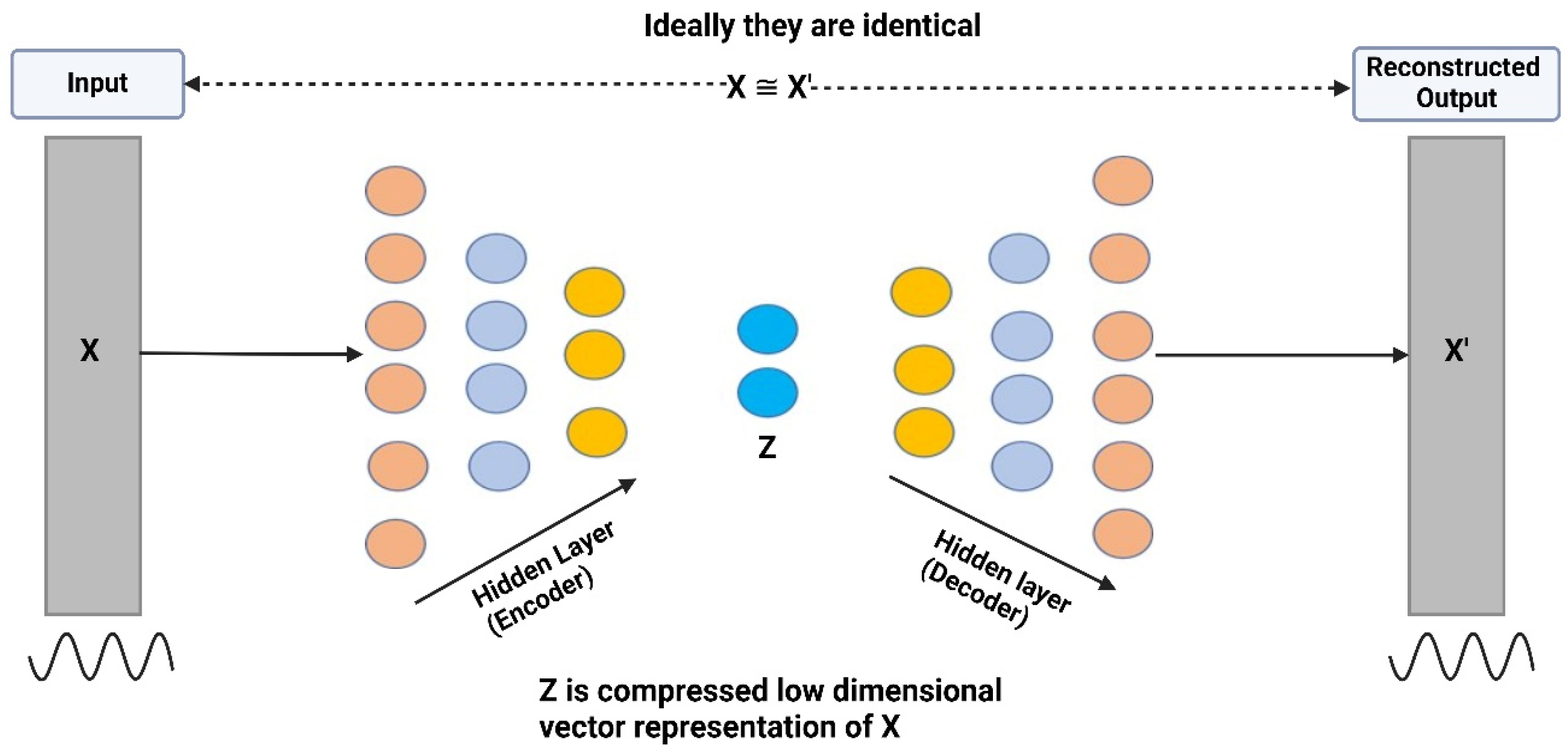
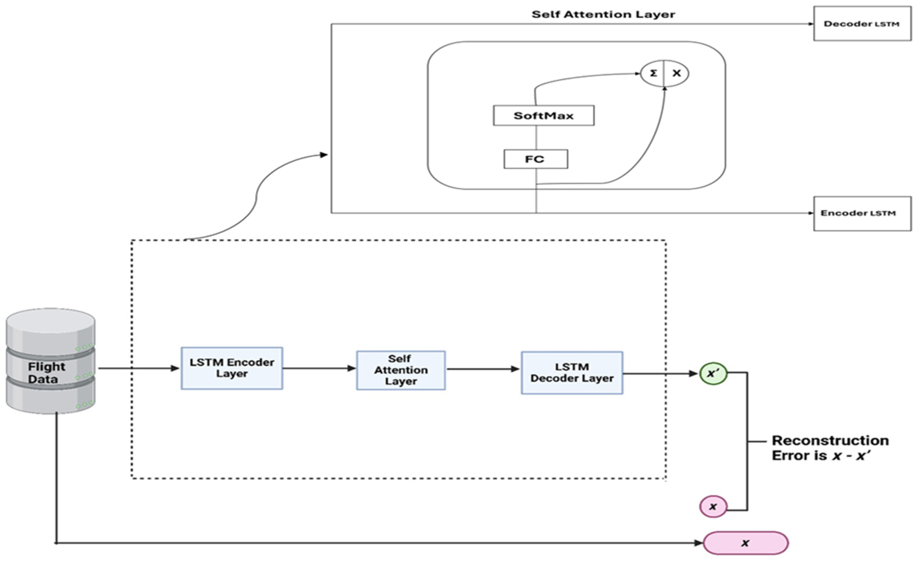
3.4.1. Autoencoder Architecture

The idea of Autoencoder originated in the 1980s and later promoted by the seminal paper [21]. The primary aim of the autoencoder is predominantly centered on the reduction in the dimensionality of the input data to reduce the complexity of the dataset by minimizing the number of features, while preserving the fundamental characteristics of the original data. This aim is achieved internally through the utilization of hidden layer(s) designated as the encoder, which proficiently compresses the input data into a more simplified and concise vector representation. Thereafter, this condensed vector representation can be reconstructed via an additional set of hidden layer(s), termed as the decoder, to produce output data that corresponds with the dimensions of the initial input data. Both the encoder and decoder elements are composed of a series of neural network layers, including structures like Recurrent Neural Networks (RNN) and Convolutional Neural Networks (CNN), among others. If the characteristics of the input data were entirely independent from one another, the challenges of compressing and later reconstructing the data would be substantial. However, in cases where the data reveals a certain degree of inherent (underlying) structure such as correlations between input features, this structure can be captured and leveraged as the input passes through the hidden layer(s). The process of deriving crucial patterns from raw input data to create a concise knowledge representation that enhances comprehensibility and manageability is referred to as representation learning. Initially designed for the purpose of diminishing the dimensionality of input data, an autoencoder framework was subsequently modified to support representation learning in an unsupervised fashion. Throughout the evolution of this domain, various autoencoder network architectures have been formulated to serve a multitude of objectives, coinciding with progress in the realm of deep learning. Figure 3 delineates the architecture of the autoencoder as discussed above.

It has been noted that x, the preliminary time series data, undergoes encoding to yield a compact representation z that exhibits a reduced dimensionality compared to x. Following this process, z is subsequently decoded to produce x′, which serves as the reconstructed version of the original input. Both x and x′ are characterized by an equivalent dimensionality and are anticipated to be theoretically indistinguishable. Consequently, an autoencoder is constructed to optimize the training of x and x′ to achieve a state of near equivalence, with the divergence being quantified through reconstruction error. An autoencoder is employed in this paper for the objective of identifying anomalies within a flight data. The architecture of the hidden layers, comprising the encoder and decoder for anomaly detection, is characterized by an hourglass configuration. The encoder is designed with a diminishing number of neurons, facilitating the generation of a compressed, low-dimensional representation of the input, whereas the decoder features an increasing number of neurons to perform the reconstruction process, yielding the output as depicted in Figure 3. The compressed vector representation z of the input and its subsequent reconstruction x’ are integral to the efficacy of this task. Figure 4 summarizes the procedural steps undertaken to train the autoencoder for the detection of anomalies in the flight data.

The hybrid Local Outlier Factor (LOF) algorithm [2] employs historical flight data from three distinct tail numbers and airports to classify flights as either normal or anomalous. The presence of three unique tail numbers denotes three individual aircraft, thus introducing variability within the dataset. This count is deliberately maintained at a minimal level to avert excessive complexity in the model. 80% of the flights classified as normal are subjected to processing within an autoencoder framework. The remaining 20% of the normal flights are designated for the purpose of model validation. In this paper, all the deep learning models were trained using a dataset comprising 2189 normal flights from three unique tail numbers, where 1751 flights (80%) were set aside for training and 438 flights (20%) were reserved for model validation. The autoencoder effectively compresses the 2189 normal flights into a compact vector representation, which is subsequently reconstructed. During the process of reconstructing these normal flights, a reconstruction error emerges. The maximum reconstruction error is utilized as the threshold for anomaly detection owing to its acceptability as the highest conceivable error. The autoencoder is subsequently validated using flight data from the validation dataset, and this procedure is reiterated until the desired threshold is attained. It is anticipated that standard flights within this dataset will demonstrate a reconstruction error that remains below the established threshold. The model is then assessed using previously saved anomalous flights, with the expectation that these anomalous flights will exceed the defined threshold. This phenomenon arises due to the fact that the autoencoder architecture has not been subjected to training on anomalous flight instances, which deviate from the normal behavioral patterns or the condensed vector representation inherent in the autoencoder framework. Consequently, autoencoders fulfill the dual function of not merely identifying anomalous flight occurrences but also facilitating dimensionality reduction and producing a compact vector representation of normative flight data, which can subsequently be utilized for a variety of applications, including predictive modeling. This paper further focuses on the methodology through which flight data is integrated into the encoding layer of the Autoencoder, as well as the diverse implications that distinct data input techniques exert on the results. This subject is elaborated upon in the subsequent subsection.

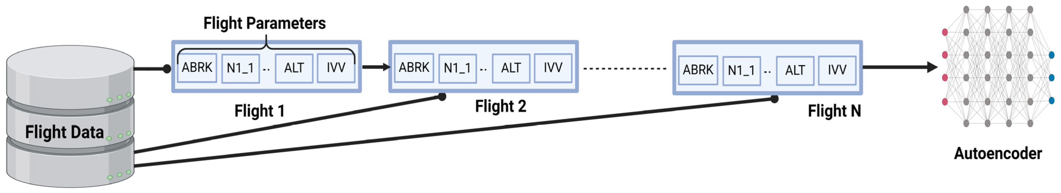
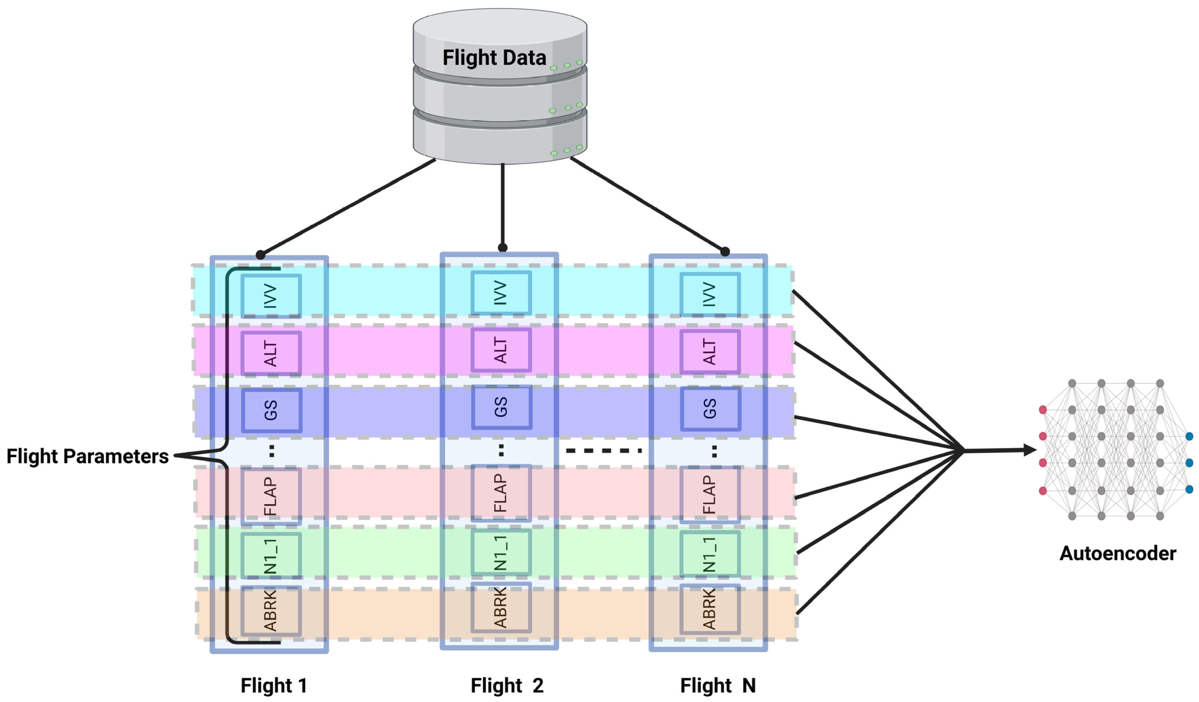
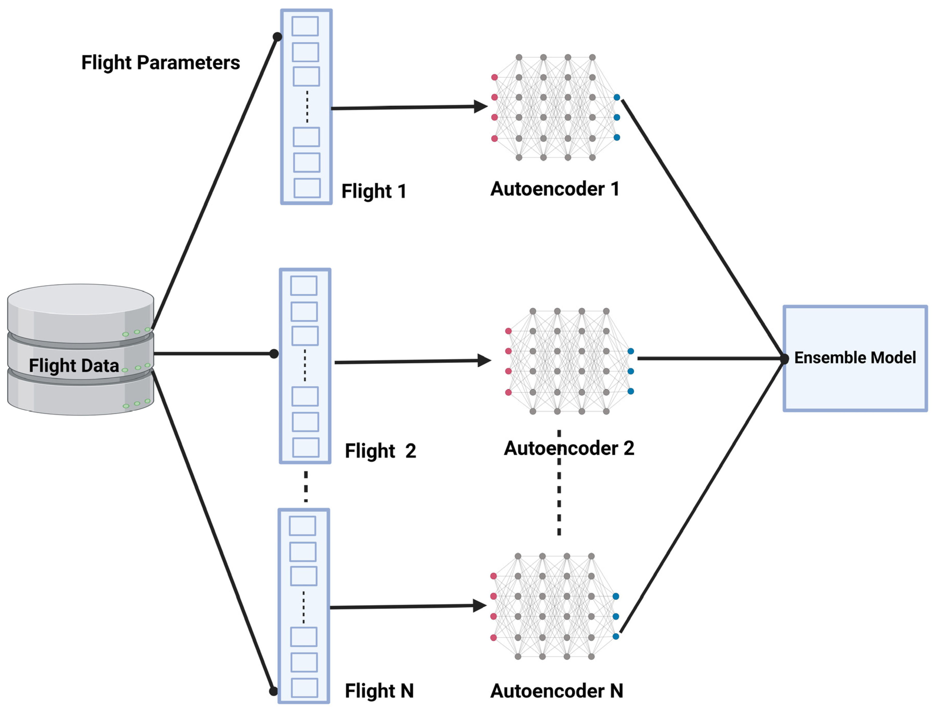
3.4.2. Formatting Flight Data for Autoencoder

From a review of existing literature, it has been observed that an array of neural network architectures has been utilized for the purposes of anomaly detection or the forecasting of time series data. However, the particular methodology pertaining to the assimilation of data within this framework remains a relatively inadequately explored and unaddressed area, especially with respect to aviation data. In this study, three discrete methodologies for the incorporation of data into the neural framework are executed.

The initial methodology encompasses the sequential input of all normal flights alongside their corresponding flight parameters into the encoding layer of the autoencoder. A single autoencoder is employed, systematically processing data from all standard flights in a sequential manner as demonstrated in Figure 5. In the subsequent methodology, similar flight parameters from all normal flights are pooled together and presented to the autoencoder in a parallel fashion, as illustrated in Figure 6. The third approach involves the concurrent feeding of each flight into its designated autoencoder cell. In this strategy, each normal flight independently trains its respective autoencoder, followed by the aggregation of the mean values derived from these discrete autoencoders for the final evaluation, as depicted in Figure 7.

For n flights, we established a corresponding n number of autoencoder units. By employing the ensemble methodology of machine learning, these units were amalgamated to produce a singular model, which was subsequently utilized to reconstruct the output. This strategy, referred to as the ensemble method, integrates the training processes of multiple models into a unified model. It has been noted that this methodology results in enhanced accuracy in the reconstruction of the original input when compared to the prior methods.

A comparative analysis of the reconstructed flight parameters utilizing the previously mentioned three methodologies is illustrated in Figure 8, Figure 9 and Figure 10, respectively. The first methodology results in a flawed reconstruction of flight parameters due to the sequential processing of each flight, leading to the dissipation of the parameter value patterns as the series lengthens. The second methodology achieves a minimal reconstruction error by maintaining the integrity of the flight parameter patterns; however, it presents a computational obstacle as it necessitates the pooling of all parameters for the model’s initial training phase. In contrast, the third methodology employs an autoencoder that is concurrently trained for each individual flight, which not only conserves time but also preserves the inherent patterns. Within this framework, the average of all models is computed to allocate equal significance to all normal flights. Consequently, the third methodology is selected to input flight data into the encoding layer of the autoencoder across all varieties of neural network architectures examined in this thesis. A comprehensive description of each neural network type is provided in the subsequent subsection, along with the accompanying results.

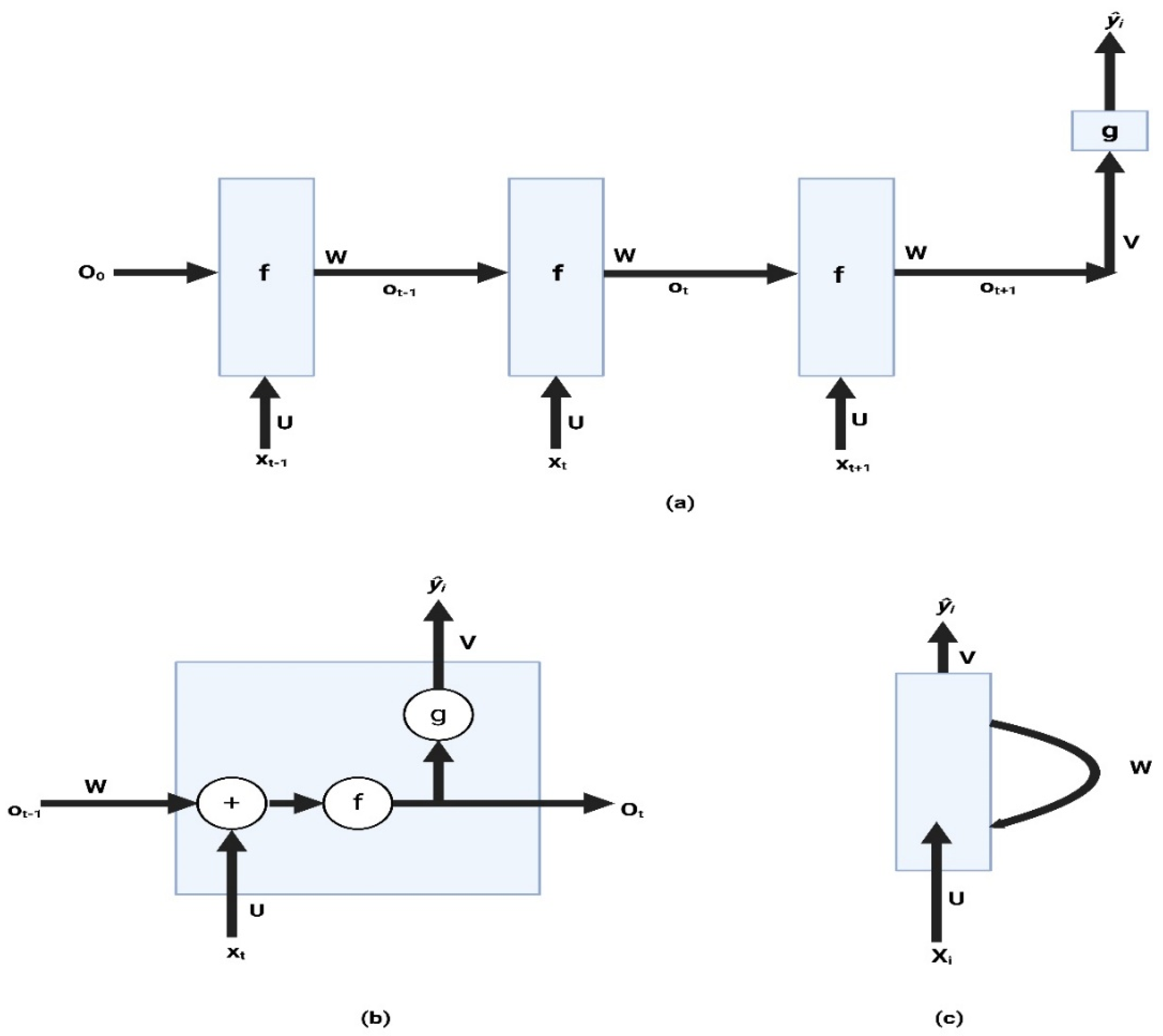
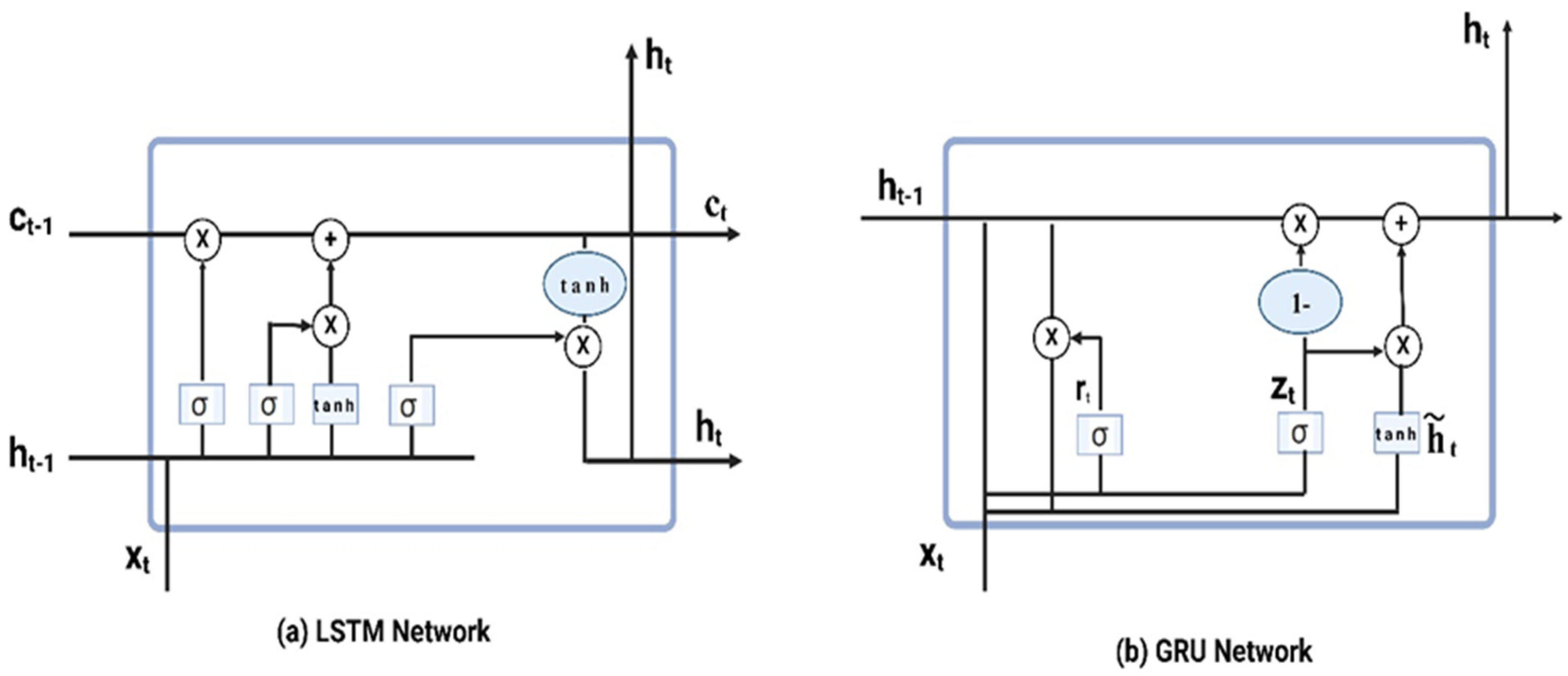
3.4.3. Neural Networks

In this paper, the hidden layers, encoder and decoder comprise layers of Neural Networks (NNs) including Recurrent Neural Networks (RNN), Convolutional Neural Networks (CNN), Long Short-Term Memory (LSTM) integrated with a self-attention mechanism and Transformer. This autoencoder framework is repeated throughout this paper employing varied configurations of the aforementioned NNs. These Neural Networks will be further examined in the following sections, along with a detailed discussion of their model architecture and the corresponding outcomes.

• Recurrent Neural Networks (RNNs)

Recurrent Neural Networks (RNNs) constitute a specialized category of neural networks that are engineered to prioritize the sequential nature of data, thereby preserving the chronology necessary for interpreting the hidden patterns inherent within a series of numerical values to achieve a specific goal. A salient benefit of RNNs is their inherent ability to accommodate and process input data sequences of varying lengths. The term ‘recurrent’ in the context of RNNs denotes a neural architecture distinguished by the systematic recurrence in the processing of information, notwithstanding the continuous influx of novel information at fixed time intervals. The architecture of Recurrent Neural Networks (RNNs), akin to all neural networks, incorporates weights and activation functions. The weights represent numerical coefficients that enhance the learning mechanism derived from the dataset. These coefficients signify the parameters that are modified throughout the training process to reduce the variance between the actual output and the desired output. The activation functions are responsible for generating the output by evaluating individual inputs alongside their associated weights. Typically, nonlinear functions such as hyperbolic tangent (tanh), Rectified Linear Unit (ReLU), and Sigmoid are employed as activation functions. This approach is implemented to incorporate complexity and to empower the network to discern intricate and nonlinear relationships present within the dataset.

Figure 11a illustrates the expanded structure of Recurrent Neural Networks (RNNs) as they handle data across three sequential time intervals called state or cell. At time step t − 1, the input x_t−1 is fed into the activation function f with input weights U, producing the output o_t−1, which is then adjusted with output weights represented as W. Subsequently, at time step t, the input x_t undergoes the same computational process. A significant aspect to note is that during the processing of input x_t, the previous state’s output is considered. Likewise, this process is reiterated for input x_t+1 at the third time step. In order to maintain architectural consistency, the initial state or cell incorporates a zero output o₀ from the preceding state, given the absence of a previous state. The final output o_t+1, accompanied by weight W, traverses through the output layer employing function g and weights V to yield the ultimate output ŷ_i. This is depicted in Figure 11b, consolidating all the time states or cells, while Figure 11c illustrates the cell with a loop, indicating the recurrent nature of the processing for each element in the input sequence. Therefore, a single layer of neural network is utilized to process newly updated information across different time intervals, rather than employing three separate layers of neural network. This efficient method greatly improves the swift processing of long sequences while maintaining their sequential coherence. Its effectiveness is rooted in its ability to directly understand the relationship between input and output sequences.

The foundational concept of deep learning is the backpropagation algorithm [22]. Essentially, it is a method that iteratively adjusts the weights of the hidden layers within the neural network to reduce the reconstruction error. The minimization of this error is depicted through a cost function of the neural network. The goal is to diminish the gradient or the rate of change in this function to an optimal level by modifying the weights and other hyperparameters in the network. At times during backpropagation, the gradients tend to decrease gradually towards zero, resulting in the weights of the initial or lower layers nearly unchanged. Consequently, the gradient descent fails to reach the optimum, known as the vanishing gradients issue. Conversely, in other scenarios, the gradients continue to amplify throughout the progression of the backpropagation process. Consequently, this leads to substantial weight updates and divergence in the gradient descent. This is known as the exploding gradients problem. Traditional RNNs encounter the issue of gradients either diminishing to zero or escalating exponentially. Long Short-Term Memory (LSTM) networks have been put forward as a solution to address the problem. The memory cells or blocks of these networks are explicitly crafted to uphold state continuity and acquire knowledge of long-term dependencies.

In Figure 12a, it is demonstrated that every LSTM cell is augmented with a distinct state vector and three distinct types of nonlinear gates, specifically the input gate, output gate and forget gate, which serve to control the movement of data into and out of the cell. X = (x₁, x₂, …, x_N) denote the inputs of LSTM cell unit, where x_t is the input vector at the time step t. σ is the sigmoid function and dot product (•) is the elementwise multiplication. Then,

i_t = σ (Wⁱx_t + Vⁱh_t−1 + Vⁱh_t−1 + bⁱ)

f_t = σ (W^fx_t + V^fh_t−1 + Vⁱh_t−1 + b^f)

o_t = σ (W^ox_t + V^oh_t−1 + Vⁱh_t−1 + b^o)

c_t = f_t • c_t−1 + i_t • tanh

where W^i, W^f, W^o, and W^c, the matrices represent the weighted values for the input gates, forget gates, output gates, and cell state, in that order and bⁱ, b^f, b^o, and b^c are their associated biases. These parameters need to be acquired during the training phase. The hidden layer vector, denoted as h_t, will serve as the input to the subsequent cell unit. The Gated Recurrent Unit (GRU), as introduced in [23], presents a simplified version of the LSTM, eliminating the need for distinct memory cells. While retaining the ability to combat the vanishing gradient issue, the GRU model demonstrates quicker training, as later demonstrated in this section. The diagram in Figure 12b depicts the gates of a GRU cell. In contrast to the LSTM cell’s three gates, the GRU cell incorporates only two gates: the updating gate z and the reset gate r. The updating gate is responsible for regulating the retained memory, while the reset gate controls the incorporation of information from the previously computed state. A reset gate value near 0 signifies the disregard of the prior state, mimicking the handling of the initial symbol in an input timestep.

In an unsupervised setting, the RNNs are implemented via autoencoder. In this research, the AE with all types of NN architecture mentioned uses mean square error (MSE) as the measure for reconstruction error (Equation (1)).

$$MSE={\displaystyle \frac{1}{n}}\sum _{i=1}^n{\left(x_i-{x\prime }_i\right)}^2$$

(1)

where n is total number of data points x_i is the input, and x′_i is the reconstructed input. LSTM, GRU, CNN, and LSTM with self-attention utilize hyperparameters listed in

Table 2. Hyperparameter selection for DL methods.

Hyperparameter	Selection
Loss Function	Mean Square Error (MSE)
Dropout	0.1
Optimizer	Adam
Learning rate	0.001
Weight decay	0.1
Number of epochs	50 or 100
Batch size	32

.

Table 3. Network architecture summary of LSTM/GRU models.

Layers	Configuration
LSTM/GRU Layer	128 Cells
LSTM/GRU Layer	64 Cells
Repeat Vector	Sequence Size = 30
LSTM/GRU Layer	64 Cells
LSTM/GRU Layer	128 Cells
Time Distributed	132

summarizes network architecture of LSTM and GRU models.

2.

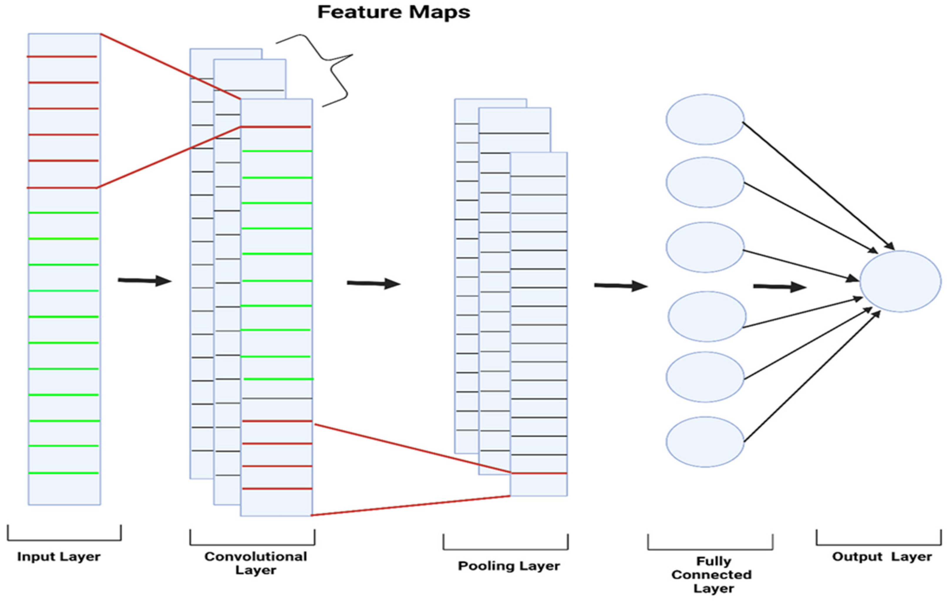
Convolutional Neural Networks (CNNs)

A standard CNN model commences with a convolutional layer designed to exploit spatial locality within a sequence. This is achieved by convolving multiple filters ( kernels) with the input data to convert raw values into more abstract patterns. Each filter is represented as a matrix, with its entries being learnt during training. These filters are then systematically shifted across the input (or time window in this context) at designated intervals known as strides. Convolutional Autoencoders, leverage Convolutional Neural Networks in both their encoder and decoder components. For time series data, a 1-d CNN Autoencoder uses windowed time-series data as an input and applies series of convolutional operations with different filter sizes to take multiple local temporal dependencies into account. Then, the results of each series of convolutions are concatenated and mapped to the latent space. Figure 13 illustrates this architecture. A similar architecture is used for both the encoder and the decoder. As a result, the decoder consists of a series of deconvolution (using Conv Transpose 1D) with different filter sizes.

Table 4. Network architecture summary of CNN model.

Layers	Configuration
Conv 1D	64 Filters, Kernel size 30
Conv 1D	32 Filters, Kernel size 30
Repeat Vector	30
ConvTranspose1D	32 Filters Kernel size 30
ConvTranspose1D	64 Filters, Kernel size 30
Time Distributed	132

summarizes network architecture of CNN model.

3.

LSTM Self-Attention Model

The “memory” of Recurrent Neural Networks (RNNs) exhibits a time-dependent characteristic, presenting both advantages and disadvantages. RNNs demonstrate a tendency to assign greater importance to recent information compared to distant historical data, resembling a weighted moving average. This characteristic proves advantageous in the context of modeling time-series data, where recent information holds more significance. Nonetheless, it also poses drawbacks in two aspects: firstly, older information tends to be disregarded even if it remains relevant and secondly, the weighting of information within a sequence may not always align solely with temporal proximity [24]. The transformer architecture has demonstrated superior efficacy compared to RNNs and convolutional (CNN) networks, especially in the domains of text translation and processing [25], as well as recently in image classification [26]. Models that rely solely on self-attention, derived from the transformer architecture, are demonstrating potential in the realm of time-series classification [27]. Attention mechanisms, initially developed for text prediction, enable the network to focus on specific parts of a sequence non-sequentially, emphasizing the significance of individual tokens in the sequence, thus enhancing the overall representation of the sequence [25]. Attention can be generally described as a weight or “context vector” of importance within a sequence [24,28]. Attention layers have emerged as a powerful tool in neural networks, enabling computers to understand and focus on important information within a sea of data. Their applications have expanded to computer vision and other domains such as time series analysis. The Transformer is a deep learning model that predominantly employs the self-attention mechanism for the purpose of modeling and omits the RNN component. The self-attention mechanism enables the model to allocate varying weights to each position within the time series, allowing it to concentrate on information from different positions during input processing. When the self-attention mechanism is integrated with LSTM architectures, it functions by encompassing all LSTM output in a sequence and establishing a distinct layer to focus on specific parts of the LSTM output more than others [29]. In anomaly detection, the attention mechanism is particularly beneficial, as not all time steps contribute equally to identifying anomalies. Specifically, time steps immediately surrounding an anomaly often contain more valuable information compared to those occurring further away. By incorporating attention, the model can effectively focus on these critical time steps, thereby improving its ability to detect anomalous events. This research implements this LSTM architecture integrated with the self-attention layer in an autoencoder to detect anomalies in flight data. The model architecture is summarised in Figure 14.

When combined with LSTM architectures, attention operates by capturing all LSTM output within a sequence and training a separate layer to “attend” to some parts of the LSTM output more than others [29]. For an input sequence x = (x₁, x₂, …, x_T) the LSTM layer produces the hidden vector sequence h = (h₁, h₂, …, h_T) and output y = (y₁, y₂, …, y_T) of the same length, by iterating the following equations from t = 1 to T.

$$h_t=H\left(W_{xh}xt+W_{hh}{h}_{t-1}+b_h\right)$$

(2)

$$y_t=\left(W_{hy}{h}_t+b_y\right)$$

(3)

where the W terms denote weight matrices, the b terms denote bias vectors, and H is the hidden layer function. In this fashion, self-attention learns to weigh portions of a sequence for relative feature importance [24].

Table 5. Network architecture summary of LSTM self-attention mechanism.

Layers	Configuration
LSTM Layer	128 Cells
LSTM Layer	64 Cells
Self-Attention Layer	64
LSTM Layer	64 Cells
LSTM Layer	128 Cells
Time Distributed	132

summarizes network architecture of LSTM self-attention model.

4.

Transformer

Transformers are deep learning models that also handle sequential data but unlike RNNs they use attention mechanisms to handle dependencies in data without recurrent layers, enabling parallel computation and capturing long-range relationships efficiently. The encoder is used to encode the input sequence while the decoder produces the output sequence [25]. The self-attention mechanism incorporated in this architecture facilitates the efficient transfer of information between the encoder–decoder pair in a bidirectional manner. Additionally, self-attention enhances the encoding of the input sequence performed by the encoder. Figure 15 illustrates a simple transformer architecture. The Transformer decouples sequence modeling from recurrence by relying entirely on attention mechanisms. It consists of an encoder stack (left) and a decoder stack (right), each repeated N times as shown in Figure 15. The following paragraph summarizes the working of Transformer.

The Transformer architecture as shown in Figure 15 consists of the following components:

• Input and Output Embeddings: This converts input tokens (time series data) into vector representations (embeddings). Positional Encoding is added to embeddings to retain the positional context of tokens. A fixed (sinusoidal) vector is added to each embedding to inject token order information.
• Encoder (left side): The first layer in encoder block is Multi-Head Attention layer. It computes multiple attention mechanisms in parallel (“heads”) to capture different contexts. Allows each token to attend to all other tokens. For each head, compute

$$Attention \left(Q,K,V\right)=softmax \left({QK}^T/\sqrt{d_k}\right)V$$

(4)

where Query (Q), Key (k) and Value (V) are linear projections of the input.

The second layer is Feed-Forward Layer. It applies fully connected layers independently to each position. Each sub-layer is wrapped with residual connection (Add) adds input back into output, followed by normalization (Norm) to stabilize learning. Encoder layers (multi-head attention and feed-forward) are stacked multiple times (N times) for deeper representation learning. It is represented as N×.

3.

Decoder (right side): It has three layers. The first layer is Masked Multi-Head Attention layer. It allows the model to focus only on previous positions in the output sequence, preventing it from seeing future positions. The second layer is Multi-Head Attention layer. It enables decoder to attend to encoder outputs. The third layer is Feed-Forward Layer. It has a similar function as in the encoder. Similarly to encoder, each sub-layer in decoder is wrapped up with Add & Norm. Decoder layers are also stacked multiple times (N times) for deeper representation learning. It is represented as N×.

4.

Linear Layer and Softmax: Liner layer converts decoder final outputs to the time series dimension. The role of the softmax function is to convert raw attention scores into probability distributions.

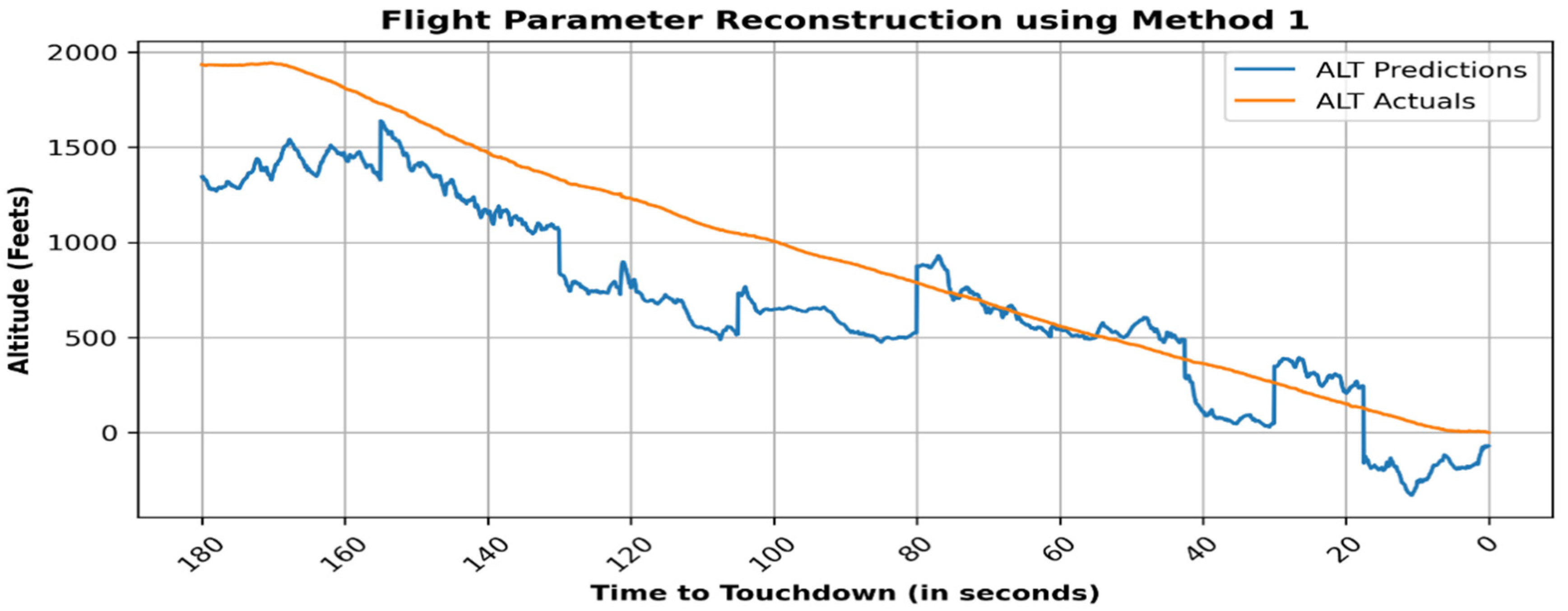
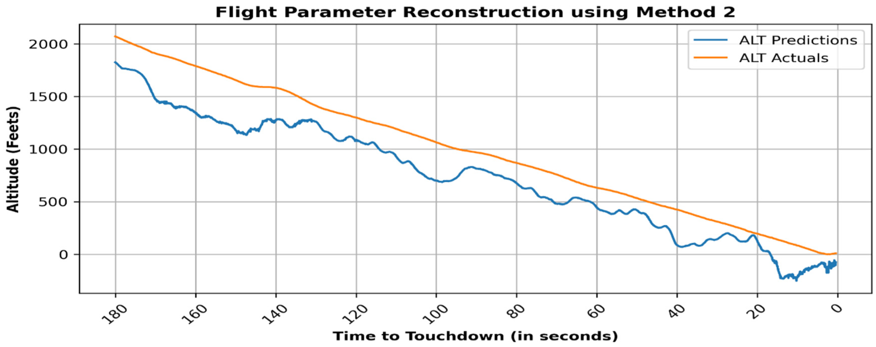
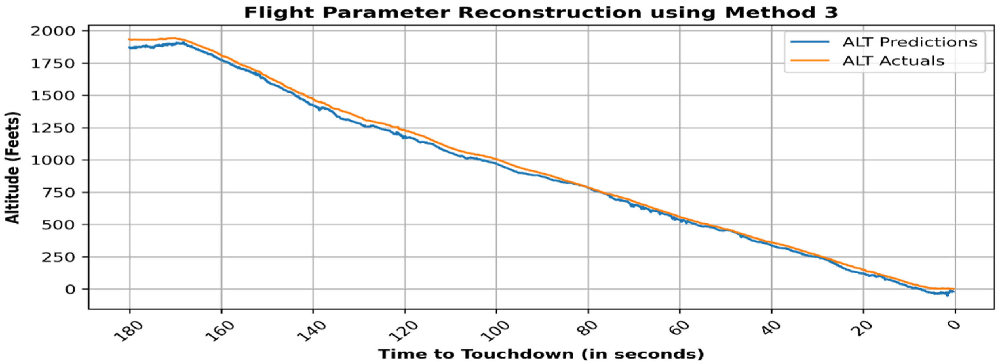
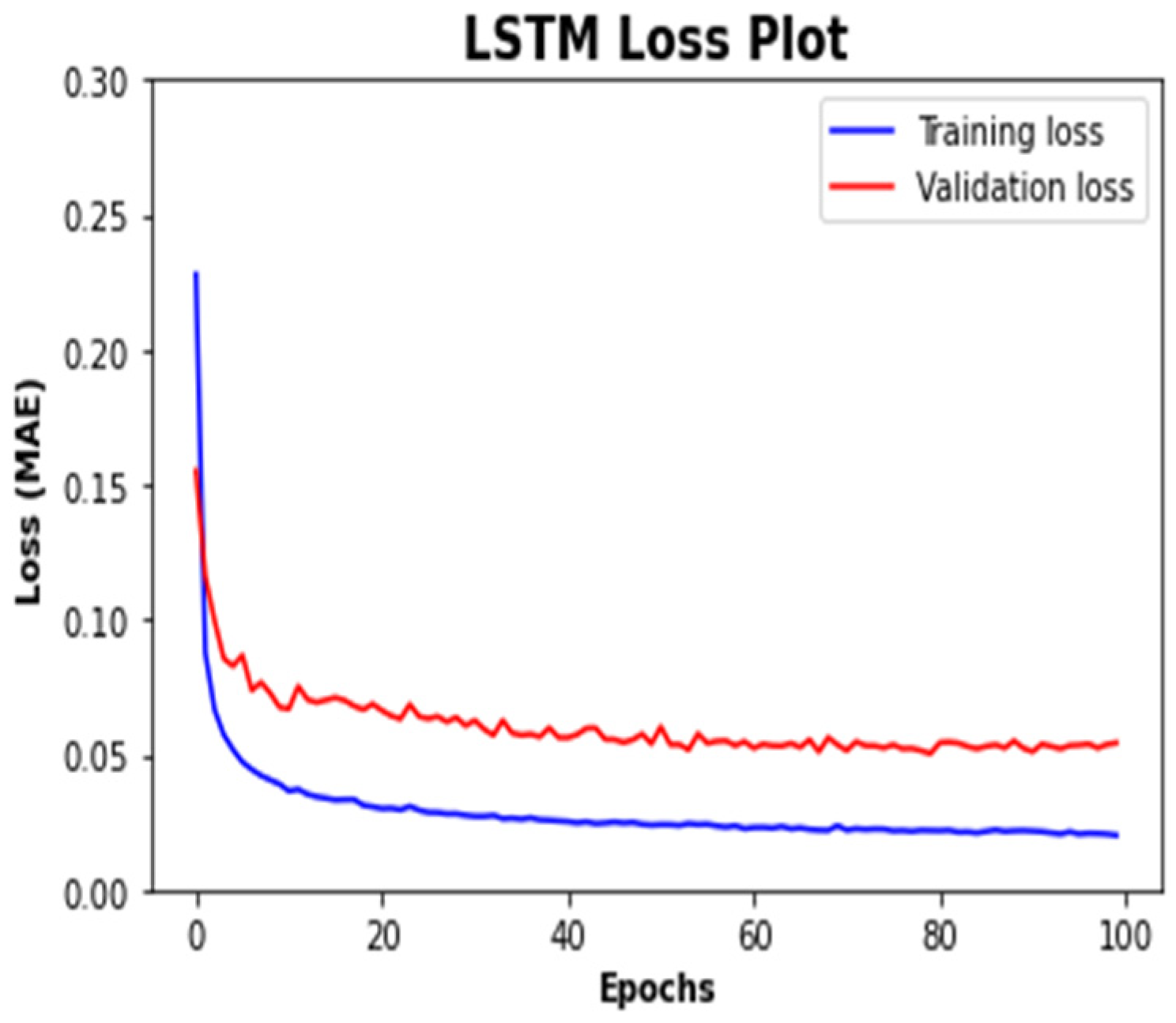
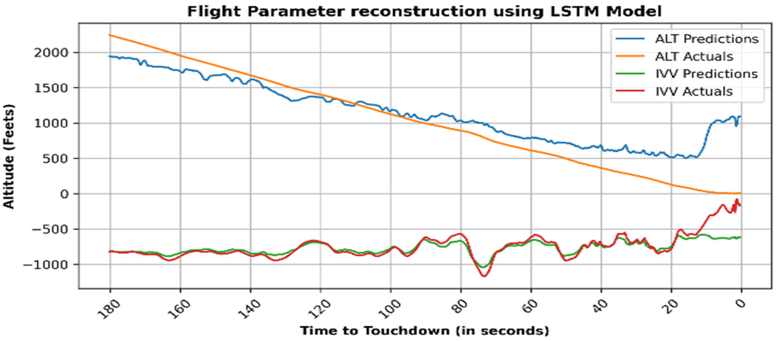
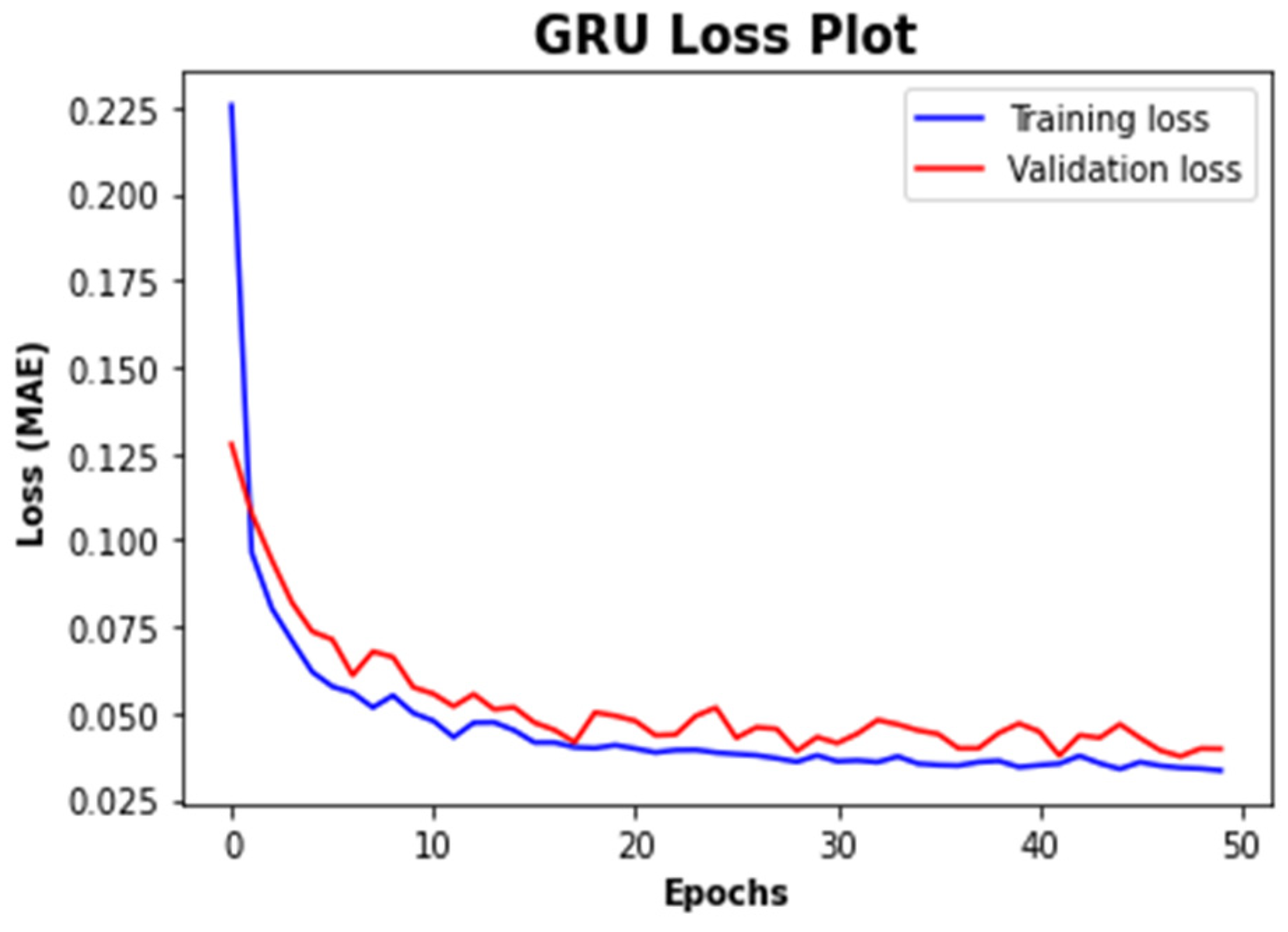
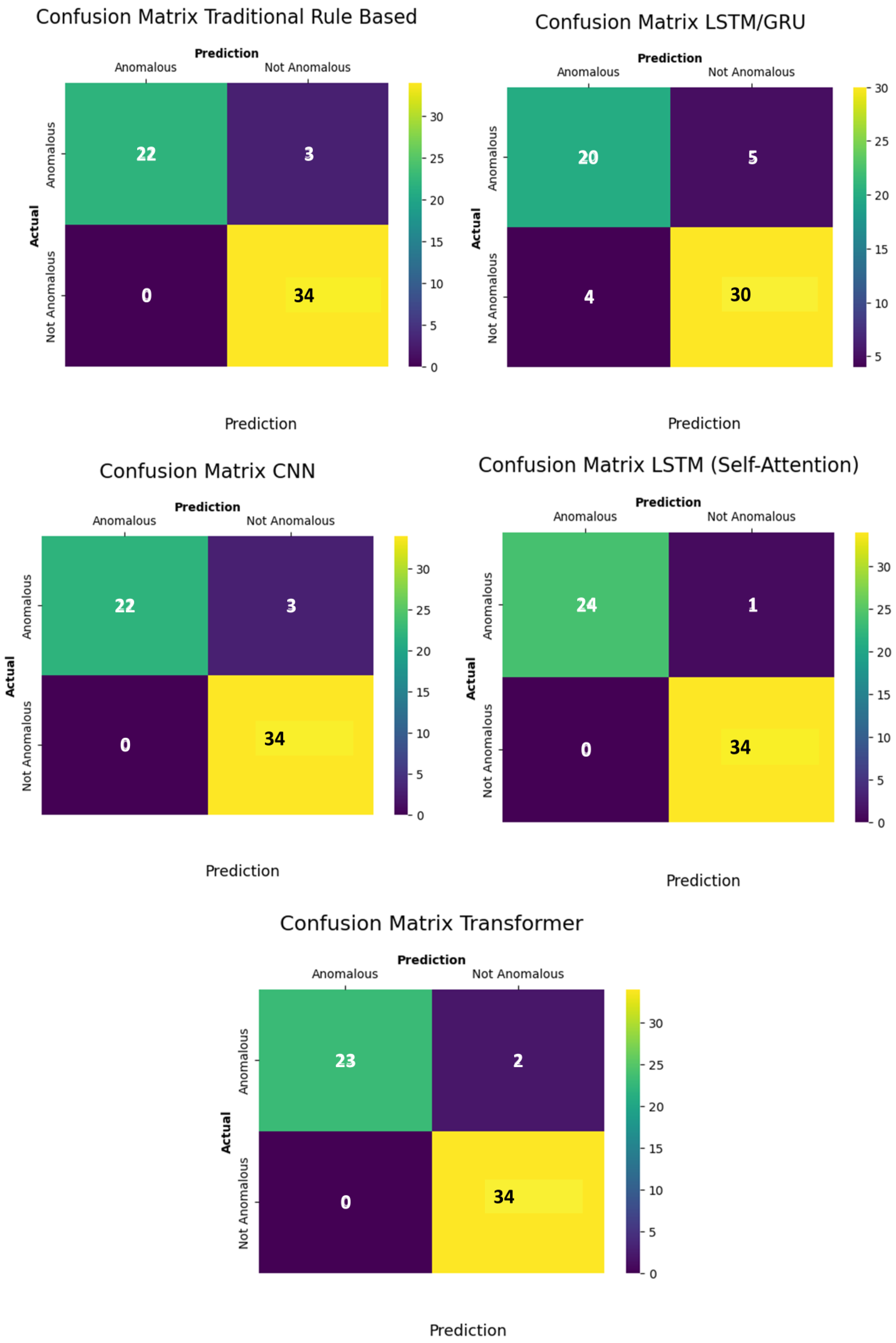
Inputs pass through embedding and positional encoding. Encoder processes inputs through multi-head self-attention and feed-forward layers. Decoder, receiving shifted outputs as inputs, applies masked self-attention and encoder–decoder attention to generate outputs. The output passes through linear and softmax layers to produce final probabilities. This structure enables Transformers to efficiently handle complex sequential tasks.

Table 6. Transformer model hyperparameters.

Category	Hyperparameter	Setup Parameter	Meaning
Model Architecture	Number of encoder layers	6	Number of transformer encoder layers
	Number of attention heads	4	Number of attention heads in the transformer self-attention mechanism
	Model dimension (d_model)	128	Size of the vector that represents each time step (or token) as it passes through the network
	Feed-forward dimension (d_ff)	512	Size of position-wise feed-forward subnetwork
	Max input sequence length	128	Maximum number of time steps (or tokens) that the Transformer will process in a single forward pass
	Positional encoding type	Sinusoidal	Pre-computed using sine and cosine functions of different frequencies:
	Loss Function	Mean Square Error (MSE)	The loss function is used to calculate the difference between the real value and the predicted value to evaluate the predictive performance of the model
Regularization	Dropout	0.1	Dropout reduces overfitting by randomly zeroing out the outputs of some neurons during training
Optimization	Optimizer	Adam	Adam is an extended algorithm for stochastic gradient descent
	Learning rate	0.001	The learning rate is the key hyperparameter used to adjust the rate of gradient descent
	Weight decay	0.1	Weight decay is to reduce overfitting by adding a penalty term to the loss function
Training	Number of epochs	50	Number of iterations
	Batch size	32	Number of independent sequence windows (here, time-series slices) processed together in one pass before updating the model’s weights

summarizes the hyperparameters used in Transformer model.

4. Results

Figure 16 shows the training and validation loss for LSTM model over 100 epochs. As explained in the beginning, 2189 flights labelled normal were considered. Out of which 1751 (roughly 80%) were used to train the LSTM model and 458 flights (20%) were used for validation purposes.

The maximum calculated MSE was 10.8. Figure 17 plots the MSE for all the 2189 normal flights reconstructed by this LSTM model.

The reconstruction of flight parameters was not accurate as the altitude parameter (ALT) failed in reconstruction whereas flight parameter Inertial Vertical Velocity (IVV) was not so accurate as seen in Figure 18.

For the GRU model, the training and validation loss over 50 epochs is shown in Figure 19. In this model also 1751 flights were used for training and 458 flights were used for validation of the model. The maximum calculated MSE was 10.3 which was less than the maximum MSE calculated for LSTM model. Figure 20 plots the MSE for all the 2189 normal flights reconstructed by this GRU model. The reconstruction of flight parameters was not accurate as the ALT as well as IVV failed in reconstruction as seen in Figure 21. The reconstruction was slightly worse than LSTM model. Figure 22 shows the training and validation loss for CNN model over 50 epochs. 2189 flights labelled normal by validated hybrid model were considered. Out of which 1751 (roughly 80%) were used to train the CNN model and 458 flights (20%) were used for validation purposes. Figure 23 plots the MSE for all the 2189 normal flights reconstructed by this CNN model. The maximum calculated MSE was 9.2, which was less than the values of LSTM and the GRU model. The reconstruction of flight parameters was slightly better than LSTM as well as GRU model. While the reconstruction of ALT parameter improved, reconstruction for IVV parameter was very accurate, as seen in Figure 24.

Figure 25 shows the training and validation loss for the LSTM self-attention model over 100 epochs. 2189 flights labeled normally by validated hybrid model were considered. Out of which 1751 (roughly 80%) were used to train this model and 458 flights (20%) were used for validation purposes. The maximum calculated MSE was 7.2 which was the lowest compared to all other models. Figure 26 plots the MSE for all the 2189 normal flights reconstructed by this model.

The reconstruction of flight parameters was accurate as compared to all other models. The reconstruction for both the parameter ALT and IVV was very accurate, as seen in Figure 27.

As the number of normal flights employed for model training rises, the mean square error (MSE) diminishes during the normal flights’ reconstruction process. Figure 28 illustrates the relationship between MSE, and the number of normal flights utilized to train the LSTM self-attention model.

Figure 29 shows the training and validation loss for Transformer model over 50 epochs. 2189 flights labelled normal by validated hybrid model were considered. Out of which 1751 (roughly 80%) were used to train the Transformer model and 458 flights (20%) were used for validation purposes. Figure 30 plots the MSE for all the 2189 normal flights reconstructed by this Transformer model. The maximum calculated MSE was 8.1 which is less than LSTM as well as GRU and CNN model but more than LSTM self-attention model. The reconstruction of flight parameters significantly outperformed both the LSTM and GRU models, as well as the CNN model as seen in Figure 31. However, when compared to the LSTM self-attention model, the reconstruction quality was not as impressive.

Five models were trained using LSTM, GRU, CNN, LSTM with self-attention layer and Transformer architecture. The LSTM with self-attention layer was determined to be the most optimal since, in this instance, the Mean Squared Error (MSE) was minimized, and the reconstruction accuracy of flight parameters was maximized. In the case of a fleet originating from different tail and airport, all models identified the same flights as anomalous. While LSTM and GRU models were specifically designed for handling long sequences, their accuracy diminishes when dealing with long sequences of multidimensional time series as in case of flight data. In contrast, CNN demonstrates superior capability in processing lengthy sequences of multidimensional time series but Transformer model outperforms all the above-mentioned models. However, it is the LSTM with a self-attention layer that achieves the highest accuracy by refining the LSTM time series modeling to concentrate on relevant segments within the extensive sequences of multidimensional time series as in case of flight data. The subsequent paragraph briefly outlines the rationale for the impressive accuracy of LSTM when integrated with a self-attention mechanism.

The Transformer model, thanks to its capability to process data concurrently, excels at managing long-distance dependencies, which enables it to perform remarkably well with sequence data. However, while the Transformer has strengths in capturing global dependencies, its effectiveness may diminish when it comes to processing local time series data [30]. To remedy this, LSTM model with self-attention mechanism is utilized. The robust temporal modeling capabilities of LSTM enhance the model’s ability to capture local temporal dependencies, thereby improving prediction accuracy. Given that flight data points are multivariate and inherently represent time series, the strengths of LSTM can be effectively leveraged to interpret and forecast this data. However, frequent fluctuations in flight parameters caused by changes in temperature, air pressure and atmospheric density across varying flight conditions [31,32] make it difficult for a single LSTM model to precisely identify key influencing factors in the current flight state. This limitation is effectively addressed by integrating an attention mechanism [33], which dynamically assigns varying degrees of emphasis within the model. This adaptability allows the model to better identify and prioritize critical factors in diverse scenarios. In this paper, the attention mechanism is utilized to enhance the identification of significant influencing factors, improve the extraction of closely related components and ultimately boost prediction accuracy.

The following section outlines the outcomes of the validation process and contrasts the results of deep learning with those obtained from traditional method.

5. Validation

For validation process 25 anomalous flights mixed with 90 normal flights were tested. The study revealed that the model, which was trained with an LSTM self-attention mechanism, accurately identified 24 out of 25 anomalous flights as confirmed by domain expert validation. There was one instance of a false negative. Figure 32 presents a qualitative analysis comparing the deep learning-based approaches with traditional techniques in relation to the ground truth. In Figure 32, flights identified as anomalous by each technique are depicted in distinct colors, while the white areas in between represent flights categorized as normal by the respective technique. The x-axis illustrates the total of 115 flights. Out of 115 flights 25 flights are true anomalies and 90 flights are normal. The y-axis enumerates all the techniques being compared. Verification by domain experts found 25 out of the 115 flights as genuine anomalies. These anomalies are highlighted in green. Secondly, 22 flights, indicated in brown, were accurately classified as anomalous by the traditional method. However, the traditional approach failed to identify 3 anomalous flights that were outside the specified parameters or boundaries outlined in Table 1. Model based on LSTM/GRU detected only 20 anomalies represented in red. All these anomalies were consistent with the ground truth. It failed to recognize 5 legitimate anomalies. Model based on CNN was able to detect 22 anomalies as shown in orange color. Transformer model was able to detect 23 anomalies as shown in cyan color. It missed 2 anomalies. LSTM with self-attention mechanism was able to detect 24 anomalies and it failed to detect 1 anomaly. Therefore, this model was most accurate amongst all DL models.

A quantitative analysis using a confusion matrix was performed. A confusion matrix aids in assessing the outcomes of each method against the ground truth. Figure 33 depicts the confusion matrix associated with each technique under investigation. The traditional rule-based method successfully identifies 22 true anomalies, known as true positives, while it fails to recognize 3 instances of anomalous flights, as illustrated in the confusion matrix. These instances are classified as false negatives. Nevertheless, it accurately detects 34 occurrences of normal flights (false positives) taken from the pool of 90 normal flights. As a result, it attains a Precision Rate (PR) of 1 and a Recall Rate (RR) of 0.88. The traditional method attains an F-1 score of 0.94. This same procedure was conducted for all DL based methods and the results are presented in

Table 7. Quantitative analysis for all techniques.

Method	Precision Rate (PR)	Recall Rate (RR)	F-1 Score
Traditional Rule Based	1.00	0.88	0.94
LSTM/GRU	0.83	0.80	0.82
CNN	1.00	0.88	0.94
LSTM (Self-Attention)	1.00	0.96	0.98
Transformer	1.00	0.92	0.96

.

LSTM self-attention technique achieved the highest overall F-1 score of 0.98. But at the same time LSTM with a self-attention mechanism experiences one instance of a false negative. In the context of anomaly detection, experiencing a false positive is preferable to encountering a false negative. This indicates that although deep learning might result in a marginally reduced accuracy because of generalization, it proves advantageous for concurrently assessing flights landing at different airports. Closely following this are the traditional rule-based method, CNN and Transformer method, which records an F-1 score of 0.94 and 0.96 respectively.

6. Conclusions

This paper compares unsupervised deep learning techniques for anomaly detection in flight data. The study applies LSTM, GRU, CNN, LSTM with a self-attention mechanism and Transformer to real-world flight data and compares their performance to traditional FDM analysis. The techniques are validated against blindfolded analysis from human experts. The findings indicate that the LSTM model incorporating a self-attention mechanism successfully identifies real anomalies, thereby achieving the highest level of prediction accuracy. The model’s ability to reconstruct flight parameters is remarkable. In contrast, LSTM, GRU, and CNN methods overlooked several anomalies that were accurately detected by the LSTM with the self-attention mechanism. Additionally, while the Transformer model is computationally demanding, it is slightly less precise than the LSTM with the self-attention mechanism. Conversely, while the traditional method relies on the existing information coming from historical knowledge, unknown issues remain unidentified. The LSTM with self-attention mechanism algorithm outperforms other DL methods in datasets due to its ability to consider crucial flight parameters in long time sequences. Consequently, it can reconstruct flight parameters more accurately. In future explorations, alternative architectural approaches for time-series analysis should be investigated alongside different self-attention mechanisms; for instance, employing sparse attention patterns, recurrence or compressed attention may significantly reduce the complexity of the self-attention layers in relation to the length of time series, while simultaneously enhancing prediction accuracy. While the current FDM system was designed to adopt a proactive approach, traditional data analysis techniques fall short of fulfilling this requirement entirely. This paper demonstrates that by incorporating deep learning-based methods, the industry can unlock substantial data potential through the generalization of the FDM process.

References

1. FAA. Airplane Flight Recorder Specifications-14 CFR 121, Appendix M. In Title 14—Aeronautics and Space; Federal Aviation Administration, Ed.; Federal Aviation Administration: Washington, DC, USA, 2011. [Google Scholar]
2. Jasra, S.K.; Valentino, G.; Muscat, A.; Camilleri, R. Hybrid Machine Learning–Statistical Method for Anomaly Detection in Flight Data. Appl. Sci. 2022, 12, 10261. [Google Scholar] [CrossRef]
3. Walker, G. Redefining the incidents to learn from: Safety science insights acquired on the journey from black boxes to Flight Data Monitoring. Saf. Sci. 2017, 99, 14–22. [Google Scholar] [CrossRef]
4. Chandola, V.; Banerjee, A.; Kumar, V. Anomaly detection. ACM Comput. Surv. 2009, 41, 1–58. [Google Scholar] [CrossRef]
5. Basora, L.; Olive, X.; Dubot, T. Recent Advances in Anomaly Detection Methods Applied to Aviation. Aerospace 2019, 6, 117. [Google Scholar] [CrossRef]
6. Aggarwal, C.C. Outlier Analysis; Springer: Cham, Switzerland, 2016; pp. 118–140. [Google Scholar] [CrossRef]
7. Pelleg, D.; Moore, A. Active learning for anomaly and rare-category detection. In Proceedings of the 17th International Conference on Neural Information Processing Systems, Vancouver, BC, Canada, 13–18 December 2004; pp. 1073–1080. [Google Scholar]
8. Megatroika, A.; Galinium, M.; Mahendra, A.; Ruseno, N. Aircraft anomaly detection using algorithmic model and data model trained on FOQA data. In Proceedings of the 2015 International Conference on Data and Software Engineering (ICoDSE), Yogyakarta, Indonesia, 25–26 November 2015. [Google Scholar]
9. Nanduri, A.; Sherry, L. Anomaly detection in aircraft data using Recurrent Neural Networks (RNN). In Proceedings of the 2016 Integrated Communications Navigation and Surveillance (ICNS), Herndon, VA, USA, 19–21 April 2016. [Google Scholar]
10. Li, L.; Das, S.; Hansman, R.; Palacios, R.; Srivastava, A. Analysis of Flight Data Using Clustering Techniques for Detecting Abnormal Operations. J. Aerosp. Inf. Syst. 2015, 12, 587–598. [Google Scholar] [CrossRef]
11. Reddy, K.; Sarkar, S.; Venugopalan, V.; Giering, M. Anomaly Detection and Fault Disambiguation in Large Flight Data: A Multi-modal Deep Auto-encoder Approach. In Proceedings of the Annual Conference of the PHM Society, Denver, CO, USA, 3–6 October 2016; Volume 8. [Google Scholar] [CrossRef]
12. Memarzadeh, M.; Matthews, B.; Avrekh, I. Unsupervised Anomaly Detection in Flight Data Using Convolutional Variational Auto-Encoder. Aerospace 2020, 7, 115. [Google Scholar] [CrossRef]
13. Alhussein, E.; Ali, A. Discovering Anomalous Patterns in Flight Data at Najaf Airport using LSTM Auto Encoders. In Proceedings of the International Iraqi Conference on Engineering Technology and Their Applications (IICETA), Najaf, Iraq, 21–22 September 2021. [Google Scholar] [CrossRef]
14. Qin, K.; Wang, Q.; Lu, B.; Sun, H.; Shu, P. Flight Anomaly Detection via a Deep Hybrid Model. Aerospace 2022, 9, 329. [Google Scholar] [CrossRef]
15. Campello, R.J.G.B.; Moulavi, D.; Sander, J. Density-Based Clustering Based on Hierarchical Density Estimates. In Advances in Knowledge Discovery and Data Mining, Proceedings of the 17th Pacific-Asia Conference, Gold Coast, Australia, 14–17 April 2013; Springer: Berlin/Heidelberg, Germany; pp. 160–172. [CrossRef]
16. Chiu, T.-Y.; Lai, Y.-C. Unstable Approach Detection and Analysis Based on Energy Management and a Deep Neural Network. Aerospace 2023, 10, 565. [Google Scholar] [CrossRef]
17. NASA. Sample Flight Data; NASA: Washington, DC, USA, 2012. Available online: https://c3.ndc.nasa.gov/dashlink/projects/85/ (accessed on 12 December 2022).
18. Airbus. A Statistical Analysis of Commercial Aviation Accidents 1958–2022. Safety First, (Issue 7 (Reference X00D17008863)), 1–36. February 2023. Available online: https://skybrary.aero/sites/default/files/bookshelf/34689.pdf (accessed on 2 December 2024).
19. Boeing. Statistical Summary of Commercial Jet Airplane Accidents 2023. Boeing. Available online: https://www.boeing.com/resources/boeingdotcom/company/about_bca/pdf/statsum.pdf (accessed on 2 October 2024).
20. Jasra, S.K.; Valentino, G.; Muscat, A.; Camilleri, R. A Comparative Study of Unsupervised Machine Learning Methods for Anomaly Detection in Flight Data: Case Studies from Real-World Flight Operations. Aerospace 2025, 12, 151. [Google Scholar] [CrossRef]
21. Hinton, G.E.; Salakhutdinov, R.R. Reducing the Dimensionality of Data with Neural Networks. Science 2006, 313, 504–507. [Google Scholar] [CrossRef] [PubMed]
22. Rumelhart, D.E.; Hinton, G.E.; Williams, R.J. Learning representations by back-propagating errors. Nature 1986, 323, 533–536. [Google Scholar] [CrossRef]
23. Chung, J.; Gulcehre, C.; Cho, K.; Bengio, Y. Empirical Evaluation of Gated Recurrent Neural Networks on SequenceModeling. arXiv 2014, arXiv:1412.3555. [Google Scholar]
24. Katrompas, A.; Ntakouris, T.; Metsis, V. Recurrence and Self-attention vs the Transformer for Time-Series Classification: A Comparative Study. In Artificial Intelligence in Medicine, Proceedings of the 20th International Conference on Artificial Intelligence in Medicine, Halifax, NS, Canada, 14–17 June 2022; Springer: Cham, Switzerland; pp. 99–109. [CrossRef]
25. Vaswani, A.; Shazeer, N.; Parmar, N.; Uszkoreit, J.; Jones, L.; Gomez, A.; Kaiser, L.; Polosukhin, I. Attention Is All You Need. In Proceedings of the Advances in Neural Information Processing Systems 30: Annual Conference on Neural Information Processing Systems 2017, Long Beach, CA, USA, 4–9 December 2017. [Google Scholar]
26. Zhao, H.; Jia, J.; Koltun, V. Exploring Self-Attention for Image Recognition. In Proceedings of the 2020 IEEE/CVF Conference on Computer Vision and Pattern Recognition (CVPR), Seattle, WA, USA, 13–19 June 2020. [Google Scholar] [CrossRef]
27. Wu, N.; Green, B.; Ben, X.; O’Banion, S. Deep Transformer Models for Time Series Forecasting: The Influenza Prevalence Case. arXiv 2020, arXiv:2001.08317. [Google Scholar] [CrossRef]
28. Bahdanau, D.; Cho, K.; Bengio, Y. Neural Machine Translation by Jointly Learning to Align and Translate. arXiv 2014, arXiv:1409.0473. [Google Scholar]
29. Lin, Z.; Feng, M.; Dos Santos, C.; Yu, M.; Xiang, B.; Zhou, B.; Bengio, Y. A Structured Self-attentive Sentence Embedding. arXiv 2017, arXiv:1703.03130. [Google Scholar] [CrossRef]
30. Shi, J.; Wang, S.; Qu, P.; Shao, J. Time series prediction model using LSTM-Transformer neural network for mine water inflow. Sci. Rep. 2024, 14, 18284. [Google Scholar] [CrossRef] [PubMed]
31. Pang, Y.; Yao, H.; Hu, J.; Liu, Y. A Recurrent Neural Network Approach for Aircraft Trajectory Prediction with Weather Features From Sherlock. In Proceedings of the AIAA Aviation 2019 Forum, Dallas, TX, USA, 17–21 June 2019. [Google Scholar]
32. Pang, Y.; Liu, Y. Conditional generative adversarial networks (CGAN) for aircraft trajectory prediction considering weather effects. In Proceedings of the AIAA Scitech 2020 Forum 1853, Orlando, FL, USA, 6–10 January 2020. [Google Scholar]
33. Jia, P.; Chen, H.; Zhang, L.; Han, D. Attention-LSTM based prediction model for aircraft 4-D trajectory. Sci. Rep. 2022, 12, 15533. [Google Scholar] [CrossRef] [PubMed]
Figure 1. Labeling of flight data and training of DL model.
Aerospace 12 00645 g001
Figure 2. Altitude (ALT) vs. time plot for synchronized flights based on time remaining to touchdown.
Aerospace 12 00645 g002
Figure 3. Architecture of an autoencoder.
Aerospace 12 00645 g003
Figure 4. Autoencoder training for anomaly detection.
Aerospace 12 00645 g004
Figure 5. Sequential architecture.
Aerospace 12 00645 g005
Figure 6. Pooled architecture.
Aerospace 12 00645 g006
Figure 7. Ensemble architecture.
Aerospace 12 00645 g007
Figure 8. Flight parameter (ALT) reconstruction using Sequential architecture (Method 1).
Aerospace 12 00645 g008
Figure 9. Flight parameter (ALT) reconstruction using Pooled architecture (Method 2).
Aerospace 12 00645 g009
Figure 10. Flight parameter (ALT) reconstruction using Ensemble architecture (Method 3).
Aerospace 12 00645 g010
Figure 11. (a) Expanded RNN architecture; (b) Consolidated RNN architecture; (c) Recurrent RNN architecture.
Aerospace 12 00645 g011
Figure 12. LSTM and GRU architectures.
Aerospace 12 00645 g012
Figure 13. Architecture of 1D CNN autoencoder.
Aerospace 12 00645 g013
Figure 14. LSTM architecture with Self-attention Layer.
Aerospace 12 00645 g014
Figure 15. A simple Transformer architecture.
Aerospace 12 00645 g015
Figure 16. Model performance of LSTM.
Aerospace 12 00645 g016
Figure 17. Mean square error (MSE) of reconstructed normal flights for LSTM model.
Aerospace 12 00645 g017
Figure 18. Actual and reconstructed flight parameters plotted by LSTM model.
Aerospace 12 00645 g018
Figure 19. Model performance of GRU.
Aerospace 12 00645 g019
Figure 20. Mean square error (MSE) of reconstructed normal flights for GRU model.
Aerospace 12 00645 g020
Figure 21. Actual and reconstructed flight parameters plotted by GRU model.
Aerospace 12 00645 g021
Figure 22. Model performance of CNN.
Aerospace 12 00645 g022
Figure 23. Mean square error (MSE) of reconstructed normal flights for CNN model.
Aerospace 12 00645 g023
Figure 24. Actual and reconstructed flight parameters plotted by CNN model.
Aerospace 12 00645 g024
Figure 25. Model performance of LSTM Self-Attention.
Aerospace 12 00645 g025
Figure 26. Mean square error (MSE) of reconstructed normal flights for LSTM self-attention model.
Aerospace 12 00645 g026
Figure 27. Actual and reconstructed flight parameters plotted by LSTM self-attention model.
Aerospace 12 00645 g027
Figure 28. MSE vs. number of normal flights utilized to train the LSTM self-attention model.
Aerospace 12 00645 g028
Figure 29. Model performance of Transformer model.
Aerospace 12 00645 g029
Figure 30. Mean square error (MSE) of reconstructed normal flights for Transformer model.
Aerospace 12 00645 g030
Figure 31. Actual and reconstructed flight parameters plotted by Transformer model.
Aerospace 12 00645 g031
Figure 32. Anomalous Flights labelled by various techniques.
Aerospace 12 00645 g032
Figure 33. Confusion Matrix for each technique.
Aerospace 12 00645 g033