Abstract
The terminal maneuvering area (TMA) serves as a critical transition zone between upper enroute airways and airports, representing one of the most complex regions for managing high volumes of arrival and departure traffic. This paper presents the multi-route TMA scheduling problem as an optimization challenge aimed at optimizing TMA interventions, such as rerouting, speed control, time-based metering, dynamic minimum time separation, and holding procedures; the objective function minimizes schedule deviations and the accumulated holding time. Furthermore, the problem is formulated as a mixed-integer linear program (MILP) to facilitate finding solutions. A rolling horizon control (RHC) dynamic optimization framework is also introduced to decompose the large-scale problem into manageable subproblems for iterative resolution. To demonstrate the applicability and effectiveness of the proposed scheduling models, a hub airport—Chengdu Tianfu International Airport (ICAO code: ZUTF) in the Cheng-Yu Metroplex—is selected for validation. Numerical analyses confirm the superiority of the proposed models, which are expected to reduce aircraft delays, shorten airborne and holding times, and improve airspace resource utilization. This study provides intelligent decision support and engineering design ideas for the macroscopic-level collaborative optimization framework of the Integrated Arrival–Departure and Surface (IADS) system.
1. Introduction
The terminal maneuvering area (TMA) is a critical transitional zone between upper enroute airways and airports, serving as a controlled airspace that manages high volumes of arrivals and departures [1,2]. However, a tricky problem facing air traffic controllers is the increasing traffic demand coupled with the limited availability of airspace resources. Moreover, controllers often rely on experience and intuition to manage TMA operations. Empirical decision-making can lead to inefficient use of time slot resources, increasing potential risks and causing significant congestion [3]. Aviation authorities have been seeking new methods to better utilize existing air traffic infrastructure to manage aircraft. One effective method is TMA scheduling, which is based on the trajectory-based operations (TBOs) concept. This method involves sequencing and merging traffic by assigning required times of arrival (RTAs) at one or more fixes along a predetermined route.
The advancement of computer science and mathematical optimization has significantly contributed to the development of the aviation industry. The TMA scheduling method can automatically generate practical and feasible solutions to managing routine traffic at the tactical level. Moreover, it enables the implementation of various TMA interventions to ensure high-capacity and conflict-free operations. These interventions include optimizing the sequencing of aircraft, rerouting, vectoring, adjustments to holding procedures, and speed control, all aimed at preventing congestion while minimizing delays.
The National Aeronautics and Space Administration (NASA) is developing an integrated NextGen technology called ATM Technology Demonstration-1 (ATD-1). In ATD-1, TMA scheduling plays a crucial role in managing aircraft arrivals. Specifically, it optimizes the sequencing and scheduling of aircraft during their descent and approach phases, starting just before the top of descent and continuing to the runway [4,5]. Meanwhile, the Single European Sky ATM Research (SESAR) program has led to the deployment of an Arrival Management System (AMAN), which provides automated sequencing support for air traffic controllers to facilitate more efficient management of arrival traffic at the TMA [6,7]. However, both ATD-1 and AMAN adopt the First-Come, First-Served (FCFS) decision-making logic for managing aircraft scheduling [8]. While FCFS may be practical for managing complex airspace, it limits the level of coordination necessary for ensuring optimal decisions by each controller. On the other hand, although FCFS prioritizes simplicity and fairness, it may not continually optimize overall system efficiency and can lead to unnecessary spare capacity, ultimately resulting in inefficient utilization of time slot resources.
Over the years, several studies have been conducted to develop mathematical formulations for the TMA scheduling problem. The underlying problems can be broadly classified into three formulations (models): basic, detailed, and holistic. The main advantage of the basic model, which focuses solely on local resources such as the runway or the final approach segment, including the Point Merge System (PMS), is that it simplifies the analysis by excluding other resources. Hong proposed an optimal sequencing and scheduling algorithm for PMS, taking into account the uncertain flight times of aircraft in terminal airspace [9]. An alternative enhancement is also presented, which incorporates a holding pattern based on mixed-integer linear programming [10] and uncertain parameters [11]. Ji Ma addressed the TMA scheduling problems of airspace conflicts and airport congestion at a macroscopic level [12], where runways and terminals are modeled as resources with a specified capacity. In this work, only the total capacity of a terminal is considered, without accounting for other waypoints. Ma proposed an arrival traffic flow-optimized sequencing model for when the demand and capacity of runways and arrival entry waypoints fluctuate [13]. However, this study did not ensure the minimum separation between consecutive aircraft at all common waypoints. Barea presented an optimization model for runway assignment and aircraft trajectory selection [14]. Each segment between a clearance point and an Instrument Approach Fix (IAF), or between an IAF and a runway, is modeled as a 2D trajectory. This work could have been more realistic, as potential conflicts were not detected and resolved at the individual aircraft and TMA resource levels.
Basic models do not account for the broader dynamics of the TMA or the full set of available resources, which may lead to suboptimal performance. In contrast, detailed models can manage individual aircraft on each relevant TMA resource based on normal routes. Desai addressed the issue of static aircraft sequencing across the TMA in a mixed-mode, single-runway operating scenario [15]. The computational results indicate that overall delays can be reduced by approximately 30% compared to the FCFS method. Huo addresses the TMA scheduling problem under uncertainty, aiming to provide a robust schedule for aircraft arrivals [16]. Conflict detection and resolution are performed at waypoints within a predefined network based on predicted time information from the trajectory model. Huo also tackles the dynamic scheduling problem using the concept of Extended Arrival Management (E-AMAN), with a horizon extending up to 500 nautical miles from the destination airport. This extension enhances cooperation and situational awareness between the upstream sector control and the TMA control [17]. Cecen proposed a stochastic mixed-integer linear programming model considering wind direction uncertainties and the PMS route [18]. The advantage of this model is its flexibility in tolerating sudden changes in wind direction. Liang developed an efficient Required Navigation Performance (RNP) route network and proposed advanced modeling to handle high-density arrivals to mixed parallel runway operations in the TMA [19,20]. Gui proposed a decision support framework that integrates trajectory optimization with arrival scheduling to enhance the management of Continuous Descent Operations (CDOs) [21,22]. A novel variable neighborhood search algorithm was employed to calculate precise arrival times at each waypoint. Wayne introduced an innovative meta-heuristic algorithm that concurrently optimizes both runway aircraft sequencing and decisions within the TMA, including runway selection, speed control, the utilization of holding patterns, vectoring, and point merges [23].
Detailed models significantly improve the feasibility of scheduling strategies by managing individual aircraft across all relevant resources based on normal routes. However, a notable performance limitation lies in the reliance on normal routes, which fail to fully utilize available airspace resources. This restricts scheduling flexibility, particularly under saturated or overloaded traffic states. Fortunately, the holistic formulation overcomes these limitations by allowing aircraft to utilize alternative routes. Capozzi presented an optimization formulation to analyze the trade-offs between hybrid strategies for managing TMA operations [24,25]. The formulation simultaneously addresses a routing and scheduling problem for metroplex traffic, treating the routing options discretely while considering time as a continuous variable. Sama developed a mathematical formulation based on alternative graphs, considering various disturbance scenarios, such as multiple delayed aircraft and temporarily disrupted runways [26,27,28]. Kam proposed an alternative path modeling method for the terminal traffic flow problem using a Directed Acyclic Graph (DAG), and an Efficient Artificial Bee Colony (EABC) algorithm was proposed and evaluated against benchmark algorithms [29,30]. Moreover, the mathematical formulation of the indeterministic traffic flow model is also presented with a min–max criterion and an enhanced Benders dual decomposition method to tackle the model’s infeasibility [31,32]. However, the proposed method, which considers the holding procedure as a potential route, has some drawbacks, such as increasing the number of holding circles, adding to the model’s dimension, and raising its computational complexity. Viè proposed a mathematical formulation and a simulation framework for aircraft landing planning, which focuses on determining the optimal landing sequence and timings of aircraft while considering various uncertainties, including variations in takeoff times and wind speeds [33]. Nevertheless, it does not account for the potential impact of departing aircraft on runway availability.
Current research predominantly focuses on detailed formulations, while holistic formulations still need to be explored. Several areas warrant further investigation and refinement. First, most existing studies adopt fixed-time separation standards for leading and trailing aircraft passing through common nodes. However, this approach may not fully account for the safety requirements of actual operations, as variations in aircraft trajectories and relative speeds significantly influence the necessary separation. For instance, a faster aircraft trailing a slower one may require a more extended time separation to ensure safety. This highlights the necessity of dynamically calculating minimum time separations based on real-time flight trajectories and speed profiles. Second, terminal airspace comprises various waypoints, each with unique characteristics and operational requirements. Traditional methods often oversimplify terminal airspace by treating it as a generalized network, neglecting the detailed classification of waypoints. This simplification can lead to operational inefficiencies or increased safety risks. A more nuanced approach to waypoint categorization and management is essential for enhancing both efficiency and safety. Third, traditional formulations often include holding procedures as potential routing options. However, incorporating each additional holding circle increases model complexity, leading to higher dimensionality and longer solution times, especially in complex airspace configurations. Overcoming these challenges requires innovative formulations to improve model accuracy and computational efficiency. Thus, the contributions of this paper are the following:
- (1)
- We propose a multiple-route terminal maneuvering area (MTMA) scheduling model, designed to minimize arrival and departure schedule deviations as well as the accumulated holding time. The model incorporates a range of intervention strategies tailored to the characteristics of different waypoints, including rerouting, speed control, time-based metering, and dynamic separation time, among others.
- (2)
- We also develop a multiple-route terminal maneuvering area scheduling model that integrates holding procedures (MTMA-H). This model extends the MTMA by allowing aircraft to execute holding procedures at Terminal Fix (TF) waypoints. Unlike traditional models, where the inclusion of each additional holding procedure significantly increases complexity, our model overcomes this limitation by using a more streamlined representation of the holding constraints.
- (3)
- Both the MTMA and MTMA-H models are formulated as mixed-integer linear programs (MILPs), with nonlinear constraints transformed into linear forms. This linearization not only reduces the computational complexity but also ensures that the models can be effectively solved using commercially available solvers, such as CPLEX, which are capable of delivering globally optimal solutions.
- (4)
- The rolling horizon control (RHC) dynamic optimization framework is introduced to address complex scheduling problems. Large-scale scheduling tasks are divided into intervals, with the number of aircraft considered in each interval forming a manageable subproblem. For each subproblem, within a predefined finite window of aircraft sequences, both the current and frozen pre-scheduling sequences are taken into account.
- (5)
- Numerical simulations are conducted to evaluate the performance of the proposed scheduling models, with ZUTF within the Cheng-Yu Metroplex selected for validation. Detailed discussions on scheduling performance and computational time consumption are provided.
The remainder of this paper is organized as follows. Section 2 provides an overview of the problem and its underlying assumptions. Section 3 introduces the multiple-route scheduling mathematical programming formulations (models) proposed in our study. The effectiveness of the proposed MTMA and MTMA-H models is demonstrated through simulations in Section 4. Concluding remarks and future work are presented in Section 5. Appendix A provides theoretical foundations supporting the proposed formulations.
2. Statement
2.1. Brief Overview of Previous Work
IADS is a critical research task in next-generation air traffic management that aims to harmonize the complex and interrelated processes of arrivals and departures. In our previous work [34], we presented the development of an IADS scheduling framework, comprising a microscopic level and a macroscopic level within the Metroplex operation, as shown in Figure 1. The microscopic level provides an optimum airport runway schedule scheme to macroscopic level and focuses on runway and taxiway scheduling. The assignment of runways and operational time slots is carried out at both microscopic and macroscopic levels. The macroscopic level towards TMA scheduling and the sequencing problem involves managing aircraft flying along enroute airways to airports. One advantage of this scheduling framework is that the optimization is distributed across disjoint components, reducing the size, scope, and complexity of the problem, making it both computable and manageable. Refer to reference [34] for the comprehensive integration at both macroscopic and microscopic levels, as outlined in the component framework description. Based on the previous study, we will continue to explore advancements in the macroscopic-level aspects of TMA scheduling.
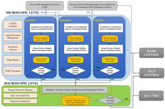
Figure 1.
IADS engineering design framework.
2.2. Problem Description
The TMA is a designated area of controlled airspace surrounding an airport. Typically, it is designed in a circular configuration, covering an area of approximately 50 to 200 nautical miles. Its primary purpose is to manage the flow of air traffic arriving at and departing from the airport, facilitating the safe and efficient coordination of high volumes of aircraft movements. During the transition from enroute to terminal airspace, aircraft arriving or departing from different gate points must be merged and organized into an orderly stream [35]. As illustrated in Figure 2, the boundary of the TMA is demarcated by Arrival Gate Points (AGPs) and Departure Gate Points (DGPs), which regulate the entry and exit of air traffic into and out of the TMA. Both arrival and departure traffic operate based on predefined procedures and routes. The route sections connecting the AGPs/DGPs to the Instrument Approach Fix are designated as Standard Terminal Arrival Routes (STARs) and Standard Instrument Departure
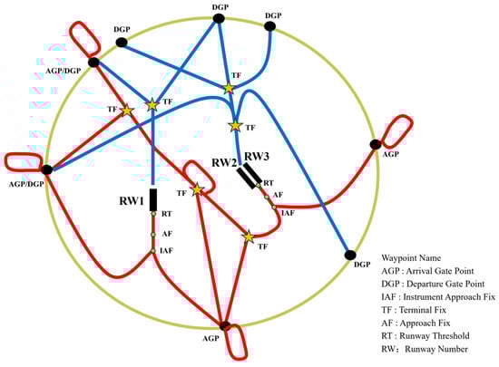
Figure 2.
TMA network structure.
Routes (SIDs), respectively. These routes comprise a series of arrival and departure segments, each connected by the Terminal Fix (TF). The approach segment is the portion of an instrument approach procedure between the Initial Approach Fix (IAF) and the runway threshold (RT), encompassing a series of Approach Fixes (AFs). At AGPs and TFs, circular flight paths are designed based on holding procedures designed to delay aircraft flights and mitigate conflicts. These procedures are organized into varying altitude levels, referred to as “stacks”, with each stack accommodating a single aircraft at a specific vertical level. Aircraft entering the holding procedure must maintain a minimum holding time. Afterward, they can exit the procedure at any time by following shorter circular or vectoring paths.
It bears noting that traffic management in the TMA is subject to a variety of constraints, including high traffic density and limited airspace resources. Consider an arriving aircraft, for example. The aircraft enters the TMA from the AGP after transferring from area control, with the TMA controller providing navigational guidance via radar vectoring. During this process, aircraft are guided by air traffic controllers, whose duty it is to ensure safe separation (see below) between aircraft and an orderly traffic flow [36]. The controllers optimize aircraft sequencing through a series of maneuvers to mitigate conflicts, including speed control, route assignment, holding procedures, and vectoring. At the IAF, descending and procedural turns are performed to align the aircraft with the AF. Controllers guide the aircraft to reach the RT. Thus, the multiple-route TMA scheduling problem can be defined. Specifically, given a set of arriving and departing aircraft, along with each aircraft’s designated route set within the TMA, its scheduled time of arrival (STA), and scheduled time of departure (STD), passing times should be assigned to each aircraft at all resource points along its chosen route (holding procedures, common segments, waypoints, and runways) in such a way that all potential conflicts are resolved and delays due to conflicting waypoints minimized.
Conflict detection, which is activated when the separation (time or distance) between two aircraft is less than a minimum separation criterion, can emphasize safety issues in the TMA. The standard lateral miles-in-trail metering between aircraft at the TF typically ranges from 3 to 5 nautical miles, depending on the airport’s ATM system performance. Time-based metering provides an efficient alternative to the traditional miles-in-trail separation and is especially beneficial when resources are constrained. At the AF and RT, stricter wake turbulence separation is specified for successively operated aircraft based on their respective categories, mitigating the impact of wake turbulence. Meanwhile, the RT must ensure the separation time for all possible aircraft scheduling combinations on the same runway, including arrival–arrival, departure–departure, departure–arrival, and arrival–departure. EUROCONTROL, NASA, and the FAA are working on recategorization (RECAT) [37], which includes time-based separation rules and lower separation requirements for consecutive aircraft, which is a calculated value based on the leading aircraft’s potential to induce turbulence and the following aircraft’s ability to withstand it. Table 1 presents the minimum wake turbulence separation rules for consecutive aircraft. In this paper, as shown in Figure 3, a variety of TMA interventions are employed to maintain high traffic volumes and ensure conflict-free operations.

Table 1.
Values for the minimum wake turbulence separation time (sec).
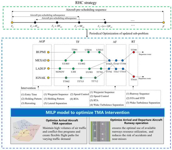
Figure 3.
TMA Scheduling Intervention.
- (i)
- Time-based metering is responsible for determining the optimal entry time at the AGP, the required time of arrival (RTA) at the TF and AF points, and STA and STD at the RT.
- (ii)
- The holding procedure involves an aircraft circling in a defined airspace while awaiting clearance to land, effectively managing lateral separation between aircraft.
- (iii)
- Rerouting refers to changing the initially planned flight route of an aircraft to avoid conflicts or to optimize air traffic flow.
- (iv)
- The waypoint sequence focuses on merging aircraft at specific waypoints or runways to achieve a more efficient aircraft sequence.
- (v)
- Speed control involves adjusting aircraft speeds to optimize target times at waypoints along the chosen routes.
- (vi)
- The dynamic separation time addresses violations of minimum lateral separation or wake turbulence separation in time between consecutive aircraft flying on the same waypoint based on their relative speeds.
We approach the multiple-route TMA scheduling problem as an optimization challenge, designed to optimize TMA interventions. Our mathematical model aims to enhance TMA and runway operations through strategies such as rerouting, time-based metering, holding procedures, and speed control to achieve optimal scheduling. The primary anticipated benefits include (i) optimizing TMA operations for arriving aircraft by ensuring high traffic volumes with conflict-free, flexible flight routes that can adapt to high-volume traffic demands, and (ii) optimizing runway operations for both arriving and departing aircraft by efficiently utilizing available slot resources, thereby enhancing safety and minimizing the risk of accidents and near misses.
2.3. Problem Assumption
Due to the limitations of classical optimization techniques, our model is developed based on several reasonable assumptions and considerations.
- (i)
- For all aircraft types, the estimated time of arrival (ETA) and estimated time of departure (ETD) are considered as prior information. Extensive research has already been conducted in this area, yielding promising predictive results [38]. ETAs and ETDs may be adjusted based on current conditions before scheduling; however, once the scheduling process begins, the ETAs and ETDs are fixed.
- (ii)
- The aircraft runway allocation results can be generated by a macroscopic-level scheduler in IADS, utilizing the method outlined in [34].
- (iii)
- Emergencies are not considered in the model, assuming a low probability of missed arrivals and departures, transgression of no-transgression zones (NTZs), pilot errors, runway incursions, and aberrant operations.
- (iv)
- Additional runway requirements or staggered separation due to unpredictable factors are ignored.
- (v)
- STAR and SID procedures are separated by altitude, with the descent profile for the STAR procedure being identical for both the leading and following aircraft.
- (vi)
- For departing aircraft, only the runway takeoff time is considered, rather than all waypoints, as departing aircraft are highly maneuverable and can resolve conflicts at other waypoints by adjusting their speed.
- (vii)
- The capacity of AGP waypoints in holding procedures is assumed to be unlimited.
- (viii)
- The potential impact of operational disruptions from neighboring airports is not considered.
Assumptions (i) and (ii) presume that the necessary information can be obtained from other systems; therefore, the details of such information are not elaborated in this paper. Assumptions (iii) and (iv) ensure that no emergency events occur during the scheduling process; in practice, such events are of very low probability. Assumptions (v) and (vi) reflect typical control practices under normal operations. Assumption (vii) considers that overloaded aircraft can generally perform ground holding, effectively rendering the AGP capacity unlimited. Assumption (viii) falls within the scope of future model research.
2.4. TMA Network Structure
Similar to the approach used in [16], the proposed modeling approach represents the terminal airspace network as a directed graph , with waypoints corresponding to intersections or holding procedures and edges denoting predetermined routes. This method enables the STAR to be concisely represented in a discretized form, incorporating information such as the locations of the waypoints and the distances. is defined as the set of waypoints, and we assume that , where is the waypoint set of the AGP, is the waypoint set of the TF, which is used to connect the AGP to the IAF, is the waypoint set of the AF used to connect the IAF to the RT, and is the waypoint at the RT. is defined as the set of edges interconnecting the aforementioned waypoints with straight-line segments, which indicate the connection of the directed graph. Each edge, , joining waypoints and , is directed to show the permissible route of an aircraft. All aircraft are elements of the set , where and denote the arriving and departing aircraft. Each aircraft is permitted to select one route from the available set of routes, , to its AGP and planned runway. We assume that represents aircraft selecting the q-th route in , which is denoted by an ordered set of waypoints . Here, the waypoints and are the virtual waypoints that, respectively, denote the origin and destination. Similarly, the predefined route is denoted by an ordered set of edges,, where and . Let the set of all edges present in all the routes of aircraft be denoted by . Specifically, the nominal route is defined as , which is derived from the regulations and historical statistics.
We now proceed by sequentially introducing the sets, parameters, and decision variables, as shown in the Nomenclature. represents the wake turbulence separation time between all potential arrival aircraft pairs at the AF as well as between all consecutive aircraft pairs (arrival–arrival, departure–departure, arrival–departure, and departure–arrival) at the RT. The decision variable defines the scheduled time for the arrival of aircraft chosen for the q-th route at the waypoint, and is the scheduled time for the departure of aircraft at the RT. is used to determine the selection of a route; this variable is used to incorporate multiple route decisions for the arriving aircraft. The binary variable indicates whether or not aircraft will perform the holding procedure at waypoint when choosing the q-th route, and defines the time limit allowed for an aircraft to remain in a holding procedure. For two aircraft, and , that overfly the same waypoint consecutively, the minimum permissible lateral separation in time are upheld by parameter at the TF. denotes the sequential relationship for consecutive aircraft pairs at waypoint .
3. Multiple-Route Scheduling Model
This section presents the MILP formulations for two scheduling models aimed at optimizing interventions in the TMA. The first model introduces the MTMA without incorporating the TF holding procedures, while the second model, MTMA-H, includes holding procedures within the scheduling framework. To address the computational challenges of large-scale problems, we employ an RHC dynamic optimization approach. A key advantage of our MILP formulation is its linear representation of all variables, which not only simplifies the model but also enables efficient, commercially available solvers, such as CPLEX, to achieve globally optimal solutions.
3.1. MTMA Scheduling Model
The innovation of the model lies in the integration of multiple-route scheduling and the consideration of time separation induced by the relative velocity of leading and trailing aircraft. Given the predefined routes and the estimated times of arrival (ETAs) and departure (ETDs) for each aircraft, the objective function consists of two components. (i) The first component minimizes deviations in the scheduled arrival and departure times relative to the estimated times. (ii) The second component aims to minimize the holding time for all aircraft. Thus, the first component of the objective function is transformed into
However, it is important to note that this objective function is expressed as the product of both logical and continuous-valued variables. By introducing an auxiliary variable , it can be converted into a linear form:
We use the big-M method, where M denotes a sufficiently large positive constant, together with a set of auxiliary constraints:
where M is the arbitrarily large number. In the MTMA model, only the holding time of the aircraft at the AGP needs to be considered; therefore, the second term of the objective function can be expressed as follows:
By setting an auxiliary variable , it can be converted into a linear form:
The additional constraint sets are subject to the following:
We set and as the weights attached to the first and second term in the objective function, respectively, and the objective function can be expressed as
Furthermore, the constraints of the MTMA are described in detail, and the mathematical formulation is provided in the following constraints. Constraint (8) ensures that each aircraft is assigned to only one route:
If an aircraft is assigned to a given route, its entry time into the TMA on that route shall be no earlier than the estimated time and no later than the maximum allowed delay:
or, equivalently, in terms of auxiliary variables:
Constraints (13) to (16), similar to the constraints defined above, impose time constraints that ensure both the arriving and departing aircraft are not scheduled earlier than the estimated times and do not exceed the maximum allowed runway delays:
Constraints (17) and (18) are used together to enforce sequence consistency, ensuring that only one aircraft is prioritized to pass through each common waypoint, thereby preventing sequencing conflicts:
Constraint (19) ensures that no overflying can occur. Any two aircraft sharing the same edge and flying in the same direction must not overtake each other:
Constraints (20) to (22) set limits on the aircraft’s arrival speed, ensuring that the aircraft operates in a decelerated state:
Constraints (23) and (24) ensure that the travel time between waypoints is greater than the minimum travel time:
It is evident that Constraint (23) is highly nonlinear and non-convex, thus cannot be solved with a guarantee of optimality. However, as shown in Lemma A1 (in Appendix A), linearization can be achieved using a well-known theorem. The linearized form of Constraints (23) and (24) can be expressed as follows:
Constraints (27) to (30) prevent violations in the separation between consecutive aircraft, ensuring that the minimum wake turbulence separation time is maintained between all possible aircraft pairs (arrival–arrival, arrival–departure, departure–arrival, and departure–departure) for the same AF or runway:
Using Lemma A2 (in Appendix A), the linearization constraints are as follows:
At each common TF waypoint, time or distance separation requirements are specified for aircraft operating in sequence. Constraint (35) defines the TMA lateral separation in time and conflict-free requirements, establishing a lower bound on the minimum required separation between each potential pair of aircraft. The leading and trailing aircraft crossing the same waypoint must maintain a time separation :
Likewise, the linearization constraints are as follows:
The traffic flows transiting through the TMA airspace network, which intersect at nodes, generate conflicts between aircraft. Time-based metering provides an efficient alternative to the current miles-in-trail metering practice. To adapt to time-based metering and ensure flight safety, it is necessary to convert distance-based separation into time-based separation. As shown in Figure 4, a node conflict occurs when horizontal separation is lost between two aircraft on two links adjacent to the same node. Let ν be a waypoint belonging to the routes of and . If the leading aircraft has greater lateral velocity than the trailing aircraft, the minimum node conflict time separation is obtained when the leading pass-through waypoint v is as follows:
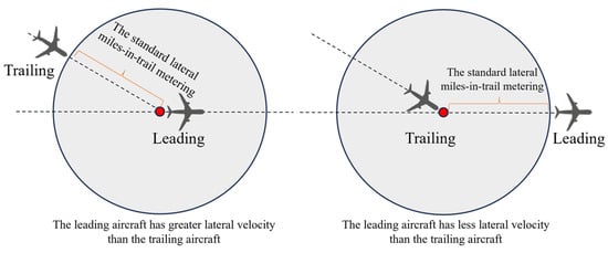
Figure 4.
Node conflict lateral separation.
If the leading aircraft has less lateral velocity than the trailing aircraft, the minimum node conflict time separation is obtained when the trailing aircraft reaches waypoint v:
By introducing a new auxiliary 0–1 variable and using Theorem A1 (in Appendix A) to express Constraints (37) and (38) linearly, we can get constraint sets as follows:
Constraint (39) shows that when is 0, it is the same as Constraint (37); when is 1, it is the same as Constraint (38). Let be an edge belonging to the routes of and . A link conflict violates the minimum lateral separation in time between two successive aircraft flying on the same link. We assume that aircraft enters the edge before , as shown in Figure 5. The lateral separation in time between the two aircraft at the edge entry waypoint must ensure no conflict at either the entry or exit waypoints while maintaining the same sequence. Thus, the following constraints need to be satisfied:
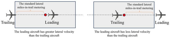
Figure 5.
Link conflict lateral separation.
By introducing an auxiliary 0–1 variable and , using Theory 2 (in Appendix A) to express Constraint (40) linearly allows us to derive the following constraint sets:
In summary, the MTMA scheduling model is represented by MILP mathematical programming formulations, including the objective function as defined in Equation (7). The constraints are specified by Equations (3), (6), (8), (11)–(22), (25), (26), (31)–(34), (36), (39), and (41). When only the nominal route is provided, i.e., , this MTMA scheduling model degenerates into a single-route TMA scheduling model.
3.2. MTMA-H Scheduling Model
Integrating the holding procedures of TMA interventions into the MTMA expands the scope of decision-making. As a result, the objective function and certain constraints are modified. The objective function must minimize the accumulated holding time for all aircraft at the AGP and TF, and Equation (7) is rewritten as follows:
By setting an auxiliary variable , the additional constraint sets are subject to the following:
This can be converted into a linear form:
Additionally, certain constraints must be revised. Initially, holding procedures are conducted at varying altitudes. If the preceding aircraft does not execute the holding procedure, the trailing aircraft is prohibited from overflying. Conversely, a trailing aircraft may overfly when the leading aircraft performs a holding procedure. Thus, Constraint (19) is modified as follows:
When is equal to 0, the constraint is equivalent to Constraint (19); when is equal to 1, the constraint allows overflight to occur. However, it is essential to ensure that any two aircraft passing the same approach segment and flying in the same direction do not overtake one another:
The travel time constraint is crucial for incorporating the supplementary holding time into the travel time between the TF waypoints. This time is calculated by summing the duration spent, subtracting the travel time, and adding any additional holding time if a holding procedure is executed at the TF waypoint. Constraints (25) to (26) will be modified as follows:
In addition, Constraints (49) and (50) ensure that the travel time between the AF waypoints is greater than the minimum possible travel time for the approach segment, and holding procedures are not permitted. Constraint (51) limits the minimum and maximum holding times for an aircraft to hold in the TF. Because controllers can apply radar vectoring for direct flights during holding procedures, the holding time constraint can be modeled as a continuous variable:
The maximum capacity constraint establishes that the holding procedure can accommodate a maximum of aircraft before leaves the waiting procedure at waypoint :
where is the indicator function, which means that if the holding time of the trailing aircraft at waypoint is exactly within interval , it is 1; otherwise, it is 0. By introducing as an auxiliary 0–1 variable, Constraint (52) can be relaxed into the following linear form constraint sets:
If is equal to 0, the capacity constraints are not applicable. Conversely, when is equal to 1 and is equal to 1, the sequential aircraft will execute the holding procedure in interval , adding 1 to the number of holds for that waypoint.
In summary, the MTMA scheduling model is represented by MILP mathematical programming formulations, including the objective function defined in Equation (42). The constraints are specified by Equations (3), (6), (8), (11)–(18), (20)–(22), (31)–(34), (36), (39), (41), (43), (45)–(50), (51), and (53). In addressing complex optimization problems, especially in the context of air traffic engineering applications, the choice of solution methods is critical to ensuring both performance and reliability. While heuristic methods such as ant colony optimization, quantum annealing, and genetic algorithms offer interesting alternatives [39,40], we have opted to integrate the CPLEX solver into our system for the advanced features for engineering optimization. Heuristic methods often require custom codes or specialized libraries, complicating system integration. Additionally, heuristic methods typically function as “black-box” algorithms, providing limited insight into the optimization process, which can make it difficult for engineers to trace or debug solutions. In contrast, CPLEX, as a standardized tool, facilitates data exchange and collaboration across engineering platforms, reducing the costs of rebuilding and maintaining complex systems.
3.3. Rolling Horizon Control Strategy
We use the CPLEX 20.1.0 solver, a commercially available software, to generate globally optimal solutions. However, this optimization problem is NP-hard, which suggests that computation times may increase exponentially as the problem size grows [41]. In practice, controllers need a solution that ensures safety and efficiency, though not necessarily one that is optimal. In the following, we propose the RHC strategy that balances solution quality with computational efficiency. The RHC provides a dynamic optimization strategy commonly used for managing complex scheduling problems. This approach involves the iterative resolution of a moving horizon for a set of aircraft. Large-scale pre-scheduling sequences are divided into intervals, with the number of aircraft considered in each interval forming manageable subsequences. For each subsequence, within a predefined finite window of aircraft sets, both the current state and predicted future conditions are considered. After implementing the initial decision, the optimized sequence is enacted, and the horizon “rolls backward”, and the process is repeated with updated interventions. Similar strategies have been successfully applied in air traffic flow management and operations research [12,19,35].
The specific flowchart of the RHC strategy designed is shown in Figure 6. The initial process of RHC decision-making can be divided into discrete aircraft pre-scheduling subsequences, each with a defined subsequence length and a freeze step of . In the RHC strategy, each subsequence consists of two groups of aircraft: the ongoing aircraft from the previous subsequence and the new aircraft arriving in the current subsequence. The arrival processes of the ongoing aircraft continue from the previous subsequence, while their interventions serve as constraints for the new aircraft. At n-th iteration, the optimization horizon is defined as , where is the first aircraft to be scheduled in the pre-scheduling sequence. Moreover, the supplementary constraints are formulated based on the freeze scheduling intervention, which replaces the pre-sequence aircraft scheduling decisions in the constraints with frozen information. Subsequently, an optimization CPLEX solver is employed to compute the optimal schedule interventions for aircraft within the specified time subsequence. Finally, aircraft are frozen in the order of runway STAs/STDs, and the subsequence is rolled backwards, repeating the process iteratively.
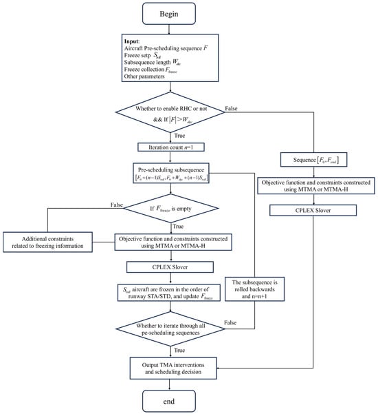
Figure 6.
The flowchart of the RHC strategy.
4. Evaluation and Results
This section presents the numerical simulations conducted to evaluate the performance of the proposed scheduling model for solving the multiple-route terminal maneuvering area scheduling problem. In order to demonstrate the universality and validity of the proposed MTMA and MTMA-H scheduling models, ZUTF within the Cheng-Yu Metroplex was selected for validation. Given the paramount importance of ensuring safety in civil aviation, prioritizing computer simulations over actual operations is essential.
4.1. Background
Chengdu Tianfu (ICAO Code: ZUTF) STARs, as outlined in the China Aeronautical Information Publication, are used to construct an airspace graph. As shown in Figure 7, the ZUUU TMA includes six AGP waypoints (MEXAD, BUPMI, AKOPI, ELDUD, IGNAK, and LADUP), two IAF waypoints (TT703 and TT904), and three RT waypoints (TT465, TT500, and TT610). Table 2 presents the complete set of routes from each AGP waypoint to the RT. For aircraft arriving from LADUP, IG-NAK, or ELDUD and destined for either TT500 or TT610, there is a single route. In contrast, AKOPI has two distinct routes, while BUPMI and MEXAD each have three.
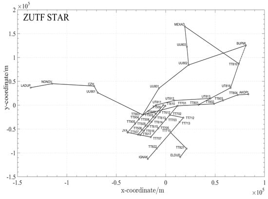
Figure 7.
The ZUTF STARs in the terminal maneuvering area.
Table 2.
Arrival routes in the ZUTF TMA.
ZUTF airport features a unique runway layout, consisting of three runways: RWY 1/19 (TT500), RWY 2/20 (TT610), and RWY 11/29 (DER 11). As shown in Figure 8, RWY 01/19 and RWY 02/20 are used for both arrivals and departures, while RWY 11 is used exclusively for departures. The runways are arranged in a “two-vertical-and-one-horizontal” configuration. Of the three runways, two are parallel to each other, and the third runway is V-shaped, opening towards the parallel runways. Specifically, the two parallel runways are separated by a distance of 2400 m, while the diverging runway has a centerline angled at 90 degrees. Eastward departures are exclusively conducted on the north runway. On RWY 01/19 and RWY 02/20, simultaneous operations can be implemented in the following modes: hybrid and semi-hybrid departures, parallel ILS approaches, and segregated arrivals/departures. During peak operations, ZUTF handles 1.20 operations per minute for arrivals and departures.
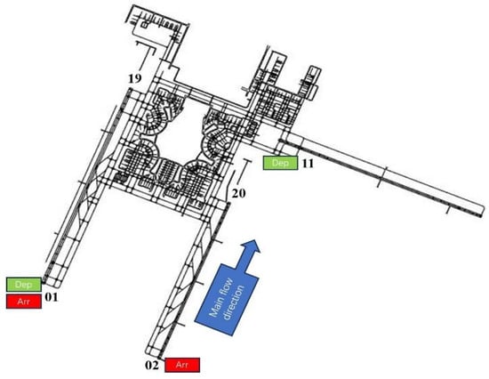
Figure 8.
Runway traffic mode for ZUTF.
It is essential to acknowledge that the scheduling problem is inherently NP-hard, implying the existence of numerous feasible solutions. To enable meaningful comparisons and ensure consistency across different experiments, it is critical to fix the experimental parameters, the selection of which is based on actual operational control rules and the level of acceptability for flight crews. Weights are attached to the first and second term in the objective function . The maximum allowable delay for the runway is s, while the terminal boundary maximum delay is s. The average speed at the TF and AF is 180 knots and 145 knots, respectively. The speed factor is 1%, 5%, 10%, and 20%, which are the minimum and maximum limits of the average speed adjustment. The maximum holding capacity is sorties, and the maximum holding time is s. The standard lateral miles-in-trail metering is . Arriving aircraft reach AGP waypoints with an estimated time that includes a random error ranging from 0 to 100 s. The maximum solution execution time is set to 60 s. The scheduling model used in the simulation presented in this paper is outlined in Table 3. The simulation data is provided by the Second Research Institute of the Civil Aviation Administration of China. The experiments were executed on a personal computer, with one Intel Core 2 Duo 2.10 GHz CPU and a 4.00 GB of RAM laptop using the CPLEX solver.
Table 3.
Introducing the simulation scheduling model.
4.2. Scheduling Results for a Test Instance
In the test instance, focusing on the pre-scheduling sequence enables a more straightforward comparison of the scheduling models without the RHC. Table 4 presents the flight plan for the test instance, which shows the scheduling of 15 aircraft (comprising 3 departing and 12 arriving aircraft) over a 14 min period, with an average of 1.07 sorties per minute. When the speed factor is , the sequencing and timing of arriving aircraft at each waypoint are as shown in Figure 9. The horizontal coordinate represents the timestamps that have undergone a day–time transformation, while the vertical coordinates are the names of the waypoints. The time separation between consecutive aircraft can be calculated as the difference between the horizontal coordinates of adjacent marks on the horizontal axis. Similarly, the travel time between waypoints can be expressed as the difference between the horizontal coordinates of the same mark. According to Constraints (39) and (41), when and , the leading and trailing aircraft crossing the same AGP and TF waypoints must satisfy the time separation of 53.55 s, and the aircraft crossing the same AF waypoint must satisfy the wake turbulence separation in Table 1. As illustrated in Figure 9A–D, all leading and trailing aircraft passing through the same waypoint comply with either the lateral or wake turbulence separation in time. Additionally, when the MTMA and MTMA-H scheduling models are applied, some aircraft arrival routes are selected as non-nominal STAR routes. Similarly, as shown in Figure 10A–D, all aircraft meet the minimum wake turbulence separation on the same runway. Furthermore, all arriving and departing aircraft adhere to the constraint of not arriving earlier than their estimated times and do not exceed the maximum allowable runway delays.
Table 4.
Test instance flight plan.
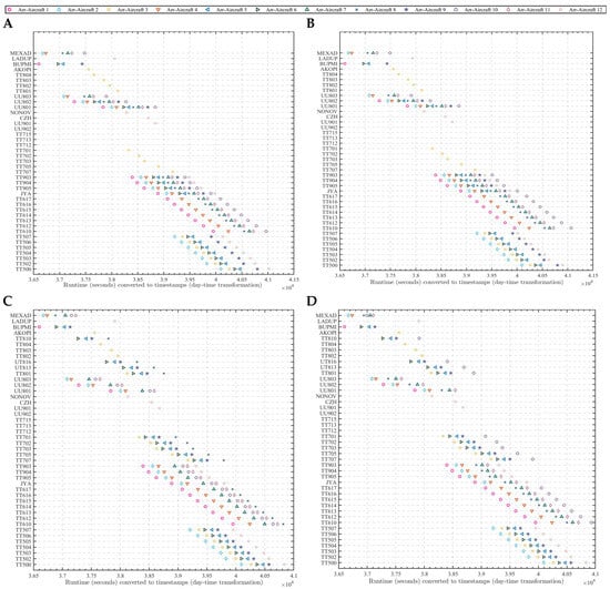
Figure 9.
The sequencing and timing of arriving aircraft at waypoints, speed factor . (A) TMA scheduling model; (B) TMA-H scheduling model; (C) MTMA scheduling model; (D) MTMA-H scheduling model.
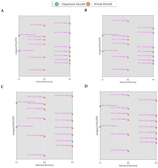
Figure 10.
The sequencing and timing of arriving and departing aircraft on runways. (A) TMA scheduling model; (B) TMA-H scheduling model; (C) MTMA scheduling model; (D) MTMA-H scheduling model.
The objective function, scheduling deviation, and accumulated holding time for the test instances are illustrated in Figure 11 to compare the scheduling performance of different scheduling models represented by distinct stacked bar segments. The objective function values for TMA and TMA-H are approximately 1488.2 s and 1469.2 s, respectively. Both models exhibit similar distributions across the metrics, with accumulated holding times () of 748 s and 738.5 s and scheduling deviations () of 740.2 s and 730.7 s, respectively. The MTMA and MTMA-H models demonstrate a significant reduction in objective function values, with values of 604.4 s and 595.1 s, respectively. Moreover, there is a noticeable decrease in the accumulated holding times (162.7 s and 126.6 s) and scheduling deviations (441.7 s and 468.5 s), indicating improved scheduling efficiency. Overall, the MTMA-H model performs best, achieving the lowest objective function value.
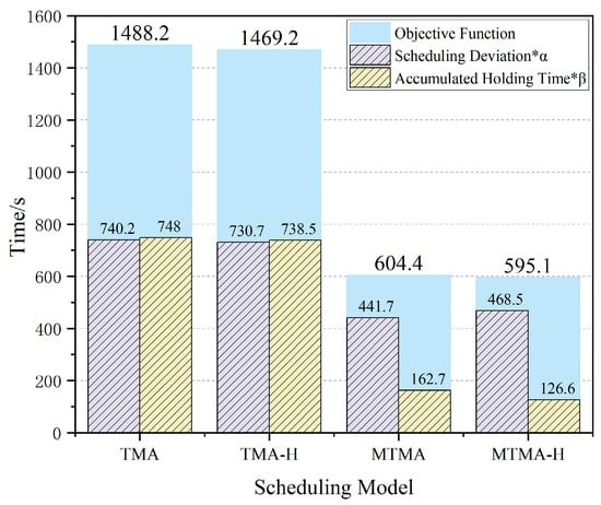
Figure 11.
Comparison of the performance of test instances for different scheduling models.
The simulation results for the test instances validate the effectiveness of the proposed models through various TMA interventions at the AGP, TF, AF, and RT waypoints. Key findings include the following: First, the TMA, TMA-H, MTMA, and MTMA-H models effectively manage the sequencing and timing of arriving aircraft to meet both lateral separation and wake turbulence separation in time constraints by utilizing interventions at the AGP, TF, AF, and RT waypoints, ensuring compliance with operational requirements. Second, the MTMA-H model demonstrates superior performance. Among the four simulation models, MTMA-H achieves the lowest objective function value, reflecting its optimal performance. The superior performance of the MTMA-H and MTMA models can be attributed to their ability to minimize prolonged holding at the AGP by selecting alternative arrival routes, thereby optimizing traffic flow and reducing delays.
4.3. Performance Analysis for Multiple Instances
To ensure the reliability of the results, the simulation is conducted in multiple instances, thereby minimizing the influence of occasional anomalies. It is worth noting that overloaded traffic conditions rarely occur in practical operations due to air traffic flow control restrictions. The purpose of this approach is to thoroughly compare the execution performance of the algorithm. The simulation has 12 operational instances, each with a set speed factor of , 5%, 10%, and 20% for a total of 48 sets of experiments. Table 5 shows that ZUTF experiences peak operations, with an average of 1.20 sorties per minute. Instances 1–2, with an average aircraft density of fewer than 0.80 sorties per minute, are classified as normal traffic states. Instances 3–7, with an average aircraft density ranging from 0.80 to 1.20 sorties per minute, are designated as saturated traffic states. Finally, instances 8–12, with an average aircraft density exceeding 1.20 sorties per minute, are categorized as overloaded traffic states. The average aircraft density in these instances exceeds that of typical operations, with most instances configured as saturated or overloaded, thus providing more opportunities to test the scheduling models’ performance. A higher proportion of medium-sized aircraft is included to better reflect actual operations. Additionally, some instances model scenarios where specific AGP points are closed due to traffic management initiatives. In instance 6, the arriving aircraft are from LADUP; in instances 5, 7, and 8, they are from MEXAD or BUPMI; and in instance 12, they are from AKOPI or BUPMI. In Figure 12, we present a comparison of the objective function values and speed factor variations across all instances for the TMA-I, TMA, TMA-H, MTMA, and MTMA-H scheduling models.
Table 5.
Instance description.
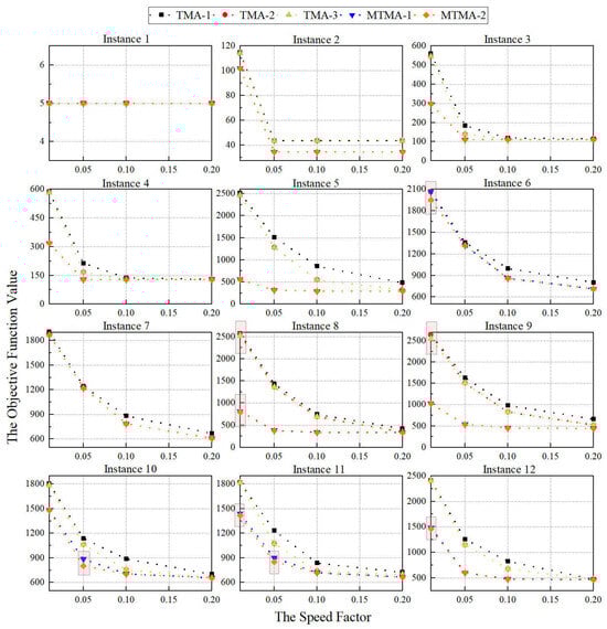
Figure 12.
Comparison results of objective function value and speed factor variation across scheduling models.
Each subplot corresponds to a specific instance, with the x-axis representing variations in the speed factor and the y-axis showing the corresponding objective function values. Several key observations can be made. First, scheduling performance improves with higher speed factors. The objective function values consistently decrease across all instances as the speed factor increases. However, higher speed factors also lead to increased control workloads. Second, the TMA-1 model demonstrates the worst performance because it restricts speed decisions to only the AGP and IAF waypoints. In contrast, other models offer more flexibility by allowing speed decisions at specific waypoints, facilitating a more effective reallocation of slot resources from leading to trailing aircraft. Third, multiple-route scheduling performs better under saturated or overloaded traffic states. In normal traffic states, the TMA and TMA-H models perform similarly to the MTMA and MTMA-H models. However, in saturated or overloaded traffic states, the TMA-H and MTMA-H models show superior performance to the TMA and MTMA models, respectively.
Interestingly, in instance 6, where all arriving aircraft are from LADUP, the performances of the TMA and MTMA models are identical, as are the performances of the TMA-H and MTMA-H models. These results align with the practical realities of air traffic control.
Furthermore, several metrics were introduced, including “Accumulated Scheduling Deviation”, “Accumulated Holding Time”, and “Airborne Time”, to quantitatively evaluate the performance of the scheduling models. In total, 48 experiments were carried out, each comprising four speed factor variations across 12 instances. As shown in Figure 13 and Figure 14, both the accumulated scheduling deviation and holding time exhibit a consistent upward trend as the number of experiments increases for all models. The TMA-I model consistently results in the highest accumulated deviation and holding time. MTMA reduced the scheduling deviation by approximately 20.49% compared to TMA-H, while MTMA-H reduced the deviation by an additional 0.57% compared to MTMA. On the other hand, MTMA-H reduced the holding time by approximately 53.5% compared to TMA and by 2.84% compared to MTMA. This comparison highlights that while MTMA-H leads to incremental improvements in reducing scheduling deviation, its impact on minimizing the holding time is far more significant. This is because the leading aircraft can stop at the TF waypoints without stopping at the AGP, and the trailing aircraft can absorb delays or deviations through other interventions. Furthermore, the scheduling deviations observed for TMA and TMA-H, as well as for MTMA and MTMA-H, are smaller, likely because a more significant number of interventions prioritize speed control instead of TF holding.
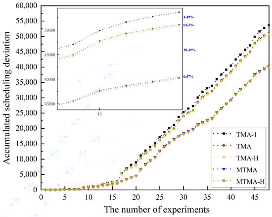
Figure 13.
Comparison of scheduling deviation for different scheduling models.
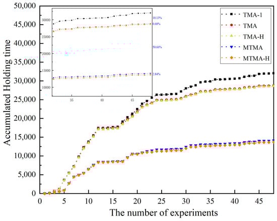
Figure 14.
Comparison of accumulated holding time for different scheduling models.
Airborne time consists of the AGP hold time and travel time, where travel time refers to the flight duration of aircraft arriving from the AGP to the RT, excluding the time spent in the AGP holding procedure. As shown in Figure 15, the mean values for the different models show little variation. The mean difference in travel time between the TMA-1 and MTMA-H models is 162.9 s, indicating that the model has a minimal effect on travel time. In contrast, as shown in Figure 16, the AGP holding time exhibits significant variation across different models. TMA-1 generally shows higher holding times than other models, while MTMA-H achieves relatively low values across all instances. With speed factor , the difference between the TMA-1 and MTMA-H holding time at the AGP is 876.46 s. With speed factor , the difference between the TMA-1 and MTMA-H holding time at the AGP is 502.08 s. Therefore, MTMA and MTMA-H have a similar travel time performance to the other models but can perform fewer holding times in the AGP, so they have less airborne time.
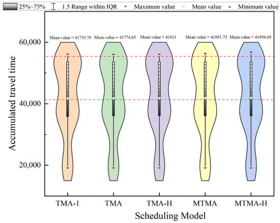
Figure 15.
Comparison of accumulated travel time for different scheduling models.
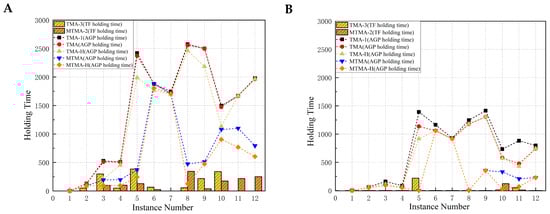
Figure 16.
AGP and TF holding times of various models in different instances. (A) Speed factor ; (B) speed factor .
As shown in Figure 16A,B, an increase in the speed factor from 1% to 5% leads to a significant reduction in AGP holding times across all scheduling models, as well as a reduction in TF holding times for both TMA-H and MTMA-H. This outcome highlights the critical role of speed factor adjustments in enhancing the efficiency of aircraft scheduling. The reduction in holding times can be attributed to the use of speed control, which frees up time slot resources.
4.4. Analysis for CPU Computing Time
We analyzed the CPU execution times of different scheduling models across all instances, including in nominal, saturated, and oversaturated traffic states, as shown in Figure 17. The maximum allowed execution time is set to 60 s, which is sufficient given that TMA scheduling occurs 15 to 30 min prior to tactical control implementation. For each instance, we performed 50 Monte Carlo simulations and recorded the average execution time. In the nominal traffic state, the execution time for all models remains under three seconds, indicating efficient performance in typical traffic conditions. However, as traffic density increases, the execution times for all models increase, with MTMA and MTMA-H exhibiting the most significant increases, especially in the oversaturated traffic state. This suggests that the introduction of multiple-route scheduling increases the complexity of the models, resulting in longer computation times. However, they still performed well within the specified time limit.
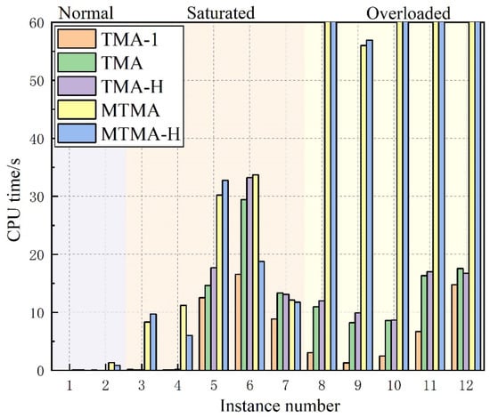
Figure 17.
Comparison of CPU computation time in different instances.
Overall, the results underscore the trade-off between model complexity and computational efficiency. While more complex route scheduling models may provide better performance in certain cases, they require significantly more computational time to converge under conditions of overloaded traffic. It is worth noting that saturated and overloaded traffic conditions rarely occur in actual operations; we set this assumption to fully compare the models’ performance.
4.5. Scheduling Results Using Rolling Horizon Control
Fortunately, for large-scale scheduling problems, the advantage of using an RHC for models that cannot achieve a globally optimal solution within the execution time is that it allows the problem to be broken down into manageable subproblems, thereby enhancing computational efficiency. However, performance is sensitive to and , with different parameter settings yielding varying results. As shown in Table 6, the findings can be categorized into the following. In instances 8 and 9, the objective function increases, indicating a decrease in performance when using an RHC. Since only a subset of the RHC is considered for decision-making, the decisions are based on incomplete information about the pre-scheduling sequence, which can lead to suboptimal solutions. In instance 10, the RHC does not significantly improve or degrade performance, possibly because the decision variables are not highly interdependent. As a result, optimizing over a short horizon has a minimal effect and does not lead to significant deviations from the global optimal solution. In instance 12, the utilization of an RHC enhances scheduling performance. This improvement may stem from the fact that, without the RHC, the model could struggle with large-scale problems, potentially becoming trapped at a local optimum or failing to converge due to the complexity of the constraints. Conversely, in instance 12, the RHC reduces the problem size, making it easier to find a superior solution. Furthermore, using instance 11 as an example, the scheduling times for both the MTMA and MTMA-H models exceeded 180 s without the RHC. However, with the implementation of the RHC, there was a remarkable reduction in scheduling time, with times decreasing to 14.64 and 19.43 s, respectively, for and . Similar conclusions were observed in other instances. These results indicate that the RHC substantially reduces computational load.
Table 6.
Scheduling results using an RHC in different instances. (The best performance indicators are in bold).
Overall, in overloaded instances, the RHC helps by reducing the problem size, making it easier to solve and improving the likelihood of finding a solution. However, the RHC is highly sensitive to the pre-scheduling sequence, leading to potential instability in solution quality. When decision variables are not highly interdependent, the RHC has little effect on performance—optimizing over a short horizon does not significantly deviate from the optimal solution.
5. Conclusions
To optimize TMA interventions, this paper presents MILP formulations for two scheduling models, MTMA and MTMA-H. To demonstrate the universality and validity of the proposed model, the hub airport ZUTF, within the Cheng-Yu Metroplex, was selected for validation. The key findings are summarized as follows.
- (1)
- The proposed models effectively manage aircraft sequencing and timing to meet lateral and wake turbulence separation in time constraints by leveraging interventions.
- (2)
- The MTMA-H model outperforms the other models, achieving incremental improvements in reducing scheduling deviation, holding time, and airborne time.
- (3)
- In the nominal traffic state, the execution times of the MTMA and MTMA-H models exhibit strong real-time computational performance. As traffic density increases, the CPU execution time for both models grows significantly. Fortunately, our proposed model continues to find better solutions than traditional methods within the time limit.
- (4)
- The performance of the RHC is highly sensitive to the specific pre-scheduling sequence and scheduling parameters. However, it is undeniable that the RHC still offers positive benefits in reducing computational time.
Our research provides comprehensive formulations for TMA scheduling. Despite these findings, inherent limitations remain, and further development is needed. Future work will extend these models to multi-airport terminal areas and explore potential operational conflicts due to shared resource preemption among airports. Meanwhile, the runway and taxiway scheduling model will be integrated into the proposed model in order to develop an IADS scheduling system capable of adapting to the dynamic nature of the TMA.
Author Contributions
C.X.: Methodology and writing—original draft; M.H.: English polishing and review editing; X.Z.: Formal analysis; Y.W.: Writing—review and editing; J.W.: Visualization; C.H.: Funding acquisition and data curation. All authors have read and agreed to the published version of the manuscript.
Funding
Special thanks go to the National Key Research and Development Program, Grant No.: 2022YFB2602400, and the Sichuan Provincial Science and Technology Support Program, Grant No.: 2022YFG0212. Furthermore, this work was supported by the Chengdu Municipal Science and Technology Program, Grant No.: 2024-YF06-00016-JH.
Data Availability Statement
The data are available from the corresponding author on reasonable request.
Acknowledgments
The authors would like to express their sincere gratitude to the Civil Aviation Administration of China Second Research Institute and the Southwest Air Traffic Management Bureau for providing the experimental data that supported this study. Their valuable contributions have greatly facilitated our research. During the preparation of this work, the authors used Grammarly software (Version 2.55) in order to check the grammar. After using this service, we reviewed and edited the content as needed and take full responsibility for the content of the publication.
Conflicts of Interest
The authors declare no conflicts of interest.
Nomenclature
| The set of aircraft, where and denote arriving and departing aircraft. | |
| The set of waypoints in the TMA airspace network model. | |
| The set of edges in the TMA airspace network model. | |
| The set of predefined routes for aircraft . | |
| The estimated time of arrival of aircraft . | |
| The estimated time of departure of aircraft . | |
| The runway maximum delay for arriving and departing aircraft. | |
| The estimated time of arrival at the terminal boundary of aircraft . | |
| The terminal boundary maximum delay for arriving aircraft. | |
| The standard lateral miles-in-trail metering between aircraft at the TF. | |
| The minimum wake turbulence separation time between aircraft (leading —trailing ) operating from the AF and RT. | |
| The weights attached to the first and second term in the objective function. | |
| The length of the edge . | |
| The minimum\maximum holding time for execution of the TF holding procedure. | |
| The maximum holding capacity taking into account controller workload. | |
| The scheduling sub-time window duration of the rolling horizon control. | |
| The step of rolling horizon control. | |
| The minimum speed for aircraft choosing the q-th route at the waypoint, where is the speed limit at the TF and is the speed at the AF. | |
| The maximum speed for aircraft choosing the q-th route at the waypoint, where is the speed limit at the TF and is the speed at the AF. | |
| Variable | |
| The binary variable: 1 if aircraft chooses the route; 0 otherwise. | |
| The binary variable: 1 if aircraft reaches the waypoint before aircraft ; 0 otherwise. | |
| The scheduled time for arrival of aircraft is chosen for the q-th route at waypoint . | |
| The scheduled time for departure of aircraft at the RT. | |
| The minimum separation between aircraft (leading —trailing ) at waypoint . | |
| The inverse of scheduled speed for aircraft is chosen for the q-th route at waypoint . | |
| The holding time for aircraft is chosen for the q-th route at waypoint . | |
Appendix A. Fundamental Theory and Lemma
Theorem A1.
where
is the auxiliary 0–1 variable and M is the arbitrarily large number.
For the original problem, if
, then
; otherwise,
, where
,
, and
are continuous variables, with
being a constant. The above constraints can be expressed linearly using the big-M method. The following set of inequalities is equivalent to the constraints:
Theorem A2.
where and
are the auxiliary 0–1 variable and M is the arbitrarily large number.
For the original problem, , where
,
, and
are continuous variables. The following set of inequalities is equivalent to the constraints:
Lemma A1.
Consider a constraint where
is a binary decision variable and A, B, C are continuous variables or constants, with
being a constant. The following linearization is equivalent to the constraint:
Proof Lemma A1.
Given that M is a sufficiently large positive integer and is a constant, the above expression can be equal to
It is not difficult to obtain,
□
Since is a binary decision variable, the following equation always holds by applying the big-M method:
Extension Lemma A1.
Consider a constraint
where
is a binary decision variable and A, B, C are continuous variables or constants, with
being a constant. The following linearization is equivalent to the constraint:
Lemma A2.
Consider a constraint
, where
,
, and
are binary decision variables and A, B are continuous variables, with
being a constant. The following linearization is equivalent to the constraint:
Proof Lemma A2.
and,
Since , , and are binary decision variables, obviously, when , this constraint always holds. When , by introducing a sufficiently large positive integer M and relaxing the constraints, Equation (A8) can be transformed into
Meanwhile, by means of Equations (9) and (10), it follows that the lower bound of satisfies the following:
When , we can get the original equation:
□
References
- Gui, X.; Zhang, J.; Tang, X.; Bao, J.; Wang, B. A data-driven trajectory optimization framework for terminal maneuvering area operations. Aerosp. Sci. Technol. 2022, 131, 108010. [Google Scholar] [CrossRef]
- Liu, W.; Delahaye, D.; Cetek, F.A.; Zhao, Q.; Notry, P. Comparison of performance between PMS and trombone arrival route topologies in terminal maneuvering area. J. Air Transp. Manag. 2024, 115, 102532. [Google Scholar] [CrossRef]
- Metzger, U.; Parasuraman, R. Automation in future air traffic management: Effects of decision aid reliability on controller performance and mental workload. In Decision Making in Aviation; Routledge: London, UK, 2017; pp. 345–360. [Google Scholar]
- Swenson, H.; Robinson, J.E., III; Winter, S. NASA’s ATM Technology Demonstration-1: Moving NextGen Arrival Concepts from the Laboratory to the Operational NAS. J. Air Traffic Control 2013, 55, 27–37. [Google Scholar]
- Swieringa, K.A.; Wilson, S.R.; Baxley, B.T.; Roper, R.D.; Abbott, T.S.; Levitt, I.; Scharl, J. Flight test evaluation of the ATD-1 interval management application. In Proceedings of the 17th AIAA Aviation Technology, Integration, and Operations Conference, Denver, CO, USA, 5–9 June 2017; p. 4094. [Google Scholar]
- Schuster, W.; Ochieng, W. Performance requirements of future Trajectory Prediction and Conflict Detection and Resolution tools within SESAR and NextGen: Framework for the derivation and discussion. J. Air Transp. Manag. 2014, 35, 92–101. [Google Scholar] [CrossRef]
- Hird, J.; Hawley, M.; Machin, C. Air traffic management security research in SESAR. In Proceedings of the 2016 11th International Conference on Availability, Reliability and Security (ARES), Salzburg, Austria, 31 August–2 September 2016; pp. 486–492. [Google Scholar]
- Bae, S.; Shin, H.S.; Lee, C.H.; Tsourdos, A. A new multiple flights routing and scheduling algorithm in terminal manoeuvring area. In Proceedings of the 2018 IEEE/AIAA 37th Digital Avionics Systems Conference (DASC), London, UK, 23–27 September 2018; pp. 1–9. [Google Scholar]
- Hong, Y.; Choi, B.; Lee, K.; Kim, Y. Dynamic robust sequencing and scheduling under uncertainty for the point merge system in terminal airspace. IEEE Trans. Intell. Transp. Syst. 2017, 19, 2933–2943. [Google Scholar] [CrossRef]
- Lee, S.; Hong, Y.; Kim, Y. Optimal scheduling algorithm in point merge system including holding pattern based on mixed-integer linear programming. Proc. Inst. Mech. Eng. Part G J. Aerosp. Eng. 2020, 234, 1638–1647. [Google Scholar] [CrossRef]
- Hong, Y.; Choi, B.; Kim, Y. Two-stage stochastic programming based on particle swarm optimization for aircraft sequencing and scheduling. IEEE Trans. Intell. Transp. Syst. 2018, 20, 1365–1377. [Google Scholar] [CrossRef]
- Ji Ma, D.; Delahaye, M.; Sbihi, P.; Scala, M.A.M. Mota, Integrated optimization of terminal maneuvering area and airport at the macroscopic level. Transp. Res. Part C Emerg. Technol. 2019, 98, 338–357. [Google Scholar]
- Ma, Y.; Hu, Y.; Li, H.; Yan, Y.; Yin, J. Aircraft rerouting and rescheduling in multi-airport terminal area under disturbed conditions. In MATEC Web of Conferences; EDP Sciences: Les Ulis, France, 2020; Volume 309, p. 03021. [Google Scholar]
- Barea, A.; de Celis, R.; Cadarso, L. Integration of airport terminal arrival route selection, runway assignment and aircraft trajectory optimisation. Transp. Res. Procedia 2020, 47, 299–306. [Google Scholar] [CrossRef]
- Desai, J.; Prakash, R. An optimization framework for terminal sequencing and scheduling: The single runway case. In Proceedings of the Complex Systems Design & Management Asia: Smart Nations–Sustaining and Designing, Proceedings of the Second Asia-Pacific Conference on Complex Systems Design & Management, CSD&M Asia 2016, Singapore, 24–26 February 2016; Springer International Publishing: Berlin/Heidelberg, Germany, 2016; pp. 195–207. [Google Scholar]
- Huo, Y.; Delahaye, D.; Sbihi, M. A probabilistic model based optimization for aircraft scheduling in terminal area under uncertainty. Transp. Res. Part C Emerg. Technol. 2021, 132, 103374. [Google Scholar] [CrossRef]
- Huo, Y. Optimization of Arrival Air Traffic in the Terminal Area and in the Extended Airspace. Ph.D. Thesis, Université Paul Sabatier-Toulouse III, Toulouse, France, 2022. [Google Scholar]
- Çeçen, R.K.; Cetek, C.; Kaya, O. Aircraft sequencing and scheduling in TMAs under wind direction uncertainties. Aeronaut. J. 2020, 124, 1896–1912. [Google Scholar] [CrossRef]
- Liang, M.; Delahaye, D.; Maréchal, P. Integrated sequencing and merging aircraft to parallel runways with automated conflict resolution and advanced avionics capabilities. Transp. Res. Part C Emerg. Technol. 2017, 85, 268–291. [Google Scholar] [CrossRef]
- Liang, M.; Delahaye, D.; Marechal, P. Conflict-free arrival and departure trajectory planning for parallel runway with advanced point-merge system. Transp. Res. Part C Emerg. Technol. 2018, 95, 207–227. [Google Scholar] [CrossRef]
- Gui, D.; Le, M.; Huang, Z.; D’Ariano, A. A Decision Support Framework for Aircraft Arrival Scheduling and Trajectory Optimization in Terminal Maneuvering Areas. Aerospace 2024, 11, 405. [Google Scholar] [CrossRef]
- Gui, D.; Le, M.; Huang, Z.; Zhang, J.; D’Ariano, A. Optimal aircraft arrival scheduling with continuous descent operations in busy terminal maneuvering areas. J. Air Transp. Manag. 2023, 107, 102344. [Google Scholar] [CrossRef]
- Ng, W.; Ribeiro, N.A.; Jorge, D. An optimization approach for the terminal airspace scheduling problem. Transp. Res. Part C Emerg. Technol. 2024, 169, 104856. [Google Scholar] [CrossRef]
- Capozzi, B.; Atkins, S.; Choi, S. Towards optimal routing and scheduling of metroplex operations. In Proceedings of the 9th AIAA Aviation Technology, Integration, and Operations Conference (ATIO) and Aircraft Noise and Emissions Reduction Symposium (ANERS), Hilton Head, SC, USA, 21–23 September 2009; p. 7037. [Google Scholar]
- Capozzi, B.; Atkins, S. A hybrid optimization approach to air traffic management for metroplex operations. In Proceedings of the 10th AIAA Aviation Technology, Integration, and Operations (ATIO) Conference, Fort Worth, TX, USA, 13–15 September 2010; p. 9062. [Google Scholar]
- Samà, M.; D’aRiano, A.; D’aRiano, P.; Pacciarelli, D. Optimal aircraft scheduling and routing at a terminal control area during disturbances. Transp. Res. Part C Emerg. Technol. 2014, 47, 61–85. [Google Scholar] [CrossRef]
- Samà, M.; D’Ariano, A.; Pacciarelli, D.; Palagachev, K.; Gerdts, M. Optimal aircraft scheduling and flight trajectory in terminal control areas. In Proceedings of the 2017 5th IEEE International Conference on Models and Technologies for Intelligent Transportation Systems (MT-ITS), Naples, Italy, 26–28 June 2017; pp. 285–290. [Google Scholar]
- Samà, M.; D’aRiano, A.; D’aRiano, P.; Pacciarelli, D. Scheduling models for optimal aircraft traffic control at busy airports: Tardiness, priorities, equity and violations considerations. Omega 2017, 67, 81–98. [Google Scholar] [CrossRef]
- Ng, K.K.H.; Lee, C.K.M.; Chan, F.T.S. An alternative path modelling method for air traffic flow problem in near terminal control area. In Proceedings of the 2019 2nd International Conference on Intelligent Autonomous Systems (ICoIAS), Singapore, 28 February–2 March 2019; pp. 171–174. [Google Scholar]
- Ng, K.H. Robust Optimisation Approaches to Airside Operations in Terminal Manoeuvring Areas. Ph.D. Thesis, Hong Kong Polytechnic University, Hong Kong, China, 2019. [Google Scholar]
- Ng, K.K.H.; Chen, C.H.; Lee, C.K.M. Mathematical programming formulations for robust airside terminal traffic flow optimisation problem. Comput. Ind. Eng. 2021, 154, 107119. [Google Scholar] [CrossRef]
- Ng, K.K.; Lee, C.K.; Chan, F.T.; Chen, C.H.; Qin, Y. A two-stage robust optimisation for terminal traffic flow problem. Appl. Soft Comput. 2020, 89, 106048. [Google Scholar] [CrossRef]
- Vié, M.S.; Zufferey, N.; Leus, R. Aircraft landing planning under uncertain conditions. J. Sched. 2022, 25, 203–228. [Google Scholar] [CrossRef]
- Xia, C.; Wen, Y.; Hu, M.; Yan, H.; Hou, C.; Liu, W. Microscopic-Level Collaborative Optimization Framework for Integrated Arrival-Departure and Surface Operations: Integrated Runway and Taxiway Aircraft Sequencing and Scheduling. Aerospace 2024, 11, 1042. [Google Scholar] [CrossRef]
- Ma, J.; Delahaye, D.; Sbihi, M.; Mongeau, M. Merging flows in terminal moneuvering area using time decomposition approach. In Proceedings of the ICRAT 2016, 7th International Conference on Research in Air Transportation, Philadelphie, PA, USA, 20–24 June 2016. [Google Scholar]
- Ikli, S.; Mancel, C.; Mongeau, M.; Olive, X.; Rachelson, E. The aircraft runway scheduling problem: A survey. Comput. Oper. Res. 2021, 132, 105336. [Google Scholar] [CrossRef]
- Xia, C.; Wu, Z.; Yang, C.; Hou, C.; Guo, C. Combining Arrival-Departure Scheduling with Runway Configuration Mode Switches. In Proceedings of the 2023 IEEE 5th International Conference on Civil Aviation Safety and Information Technology (ICCASIT), Dali, China, 11–13 October 2023; pp. 399–403. [Google Scholar]
- Yang, C.; Zhang, J.; Gui, X.; Peng, Z.; Wang, B. A data-driven method for flight time estimation based on air traffic pattern identification and prediction. J. Intell. Transp. Syst. 2024, 28, 352–371. [Google Scholar] [CrossRef]
- Haba, R.; Mano, T.; Ueda, R.; Ebe, G.; Takeda, K.; Terabe, M.; Ohzeki, M. Routing and scheduling optimization for urban air mobility fleet management using quantum annealing. Sci. Rep. 2025, 15, 4326. [Google Scholar] [CrossRef] [PubMed]
- Song, J.; Chen, C.; Heidari, A.A.; Liu, J.; Yu, H.; Chen, H. Performance optimization of annealing salp swarm algorithm: Frameworks and applications for engineering design. J. Comput. Des. Eng. 2022, 9, 633–669. [Google Scholar] [CrossRef]
- Samà, M.; D’Ariano, A.; Pacciarelli, D. Rolling horizon approach for aircraft scheduling in the terminal control area of busy airports. Procedia-Soc. Behav. Sci. 2013, 80, 531–552. [Google Scholar] [CrossRef]
Disclaimer/Publisher’s Note: The statements, opinions and data contained in all publications are solely those of the individual author(s) and contributor(s) and not of MDPI and/or the editor(s). MDPI and/or the editor(s) disclaim responsibility for any injury to people or property resulting from any ideas, methods, instructions or products referred to in the content. |
© 2025 by the authors. Licensee MDPI, Basel, Switzerland. This article is an open access article distributed under the terms and conditions of the Creative Commons Attribution (CC BY) license (https://creativecommons.org/licenses/by/4.0/).