Pressure Characteristics Analysis of the Deflector Jet Pilot Stage Under Dynamic Skewed Velocity Distribution

Abstract

The velocity distribution at the deflector jet outlet significantly influences the pressure characteristics of the pilot stage, thereby affecting the dynamic performance of the servo valve. Conventional mathematical models fail to account for the influence of dynamic velocity distribution on pilot stage pressure characteristics, resulting in significant deviations from actual situations. As the deflector shifts, the secondary jet velocity distribution transitions from a symmetric to an asymmetric dynamic profile, altering the pressure within the receiving chambers. To address this, a dynamic skewed velocity distribution model is proposed to more accurately capture the pressure characteristics. The relationship between the skewness coefficient and deflector displacement is established, and the pressure calculation method for the receiving chambers is refined accordingly. A comparative analysis shows that the proposed model aligns most closely with computational fluid dynamics results, achieving a 98% match in velocity distribution and a maximum pressure error of 1.43%. This represents an improvement of 84.98% over the normal model and 82.35% over the uniform model, confirming the superior accuracy of the dynamic skewed model in pilot stage pressure calculation.

1. Introduction

As a core part of a hydraulic system, the deflector jet servo valve (DJSV) has the advantages of strong anti-pollution, high precision, and fast dynamic response. It is widely used in aerospace, national defence, and industrial production. Therefore, improving the performance of the DJSV is of great significance [1,2,3,4]. The dynamic performance of the DJSV is significantly influenced by the pilot stage pressure characteristics. However, the pilot stage flow field is often accompanied by cavitation [5,6,7], noise [8], pressure fluctuations [9,10], self-excited oscillation [11], and other phenomena [12,13,14]. In particular, the velocity distribution at the deflector plate outlet strongly influences the pilot stage pressure characteristics. Therefore, it is necessary to establish a mathematical model based on the velocity distribution to analyse the intrinsic pressure characteristics of the pilot stage. This approach enhances understanding of pilot stage flow dynamics and provides a theoretical foundation for servo valve manufacturing, performance prediction, and the mitigation of pressure-induced instabilities.

The analysis of the pilot stage flow field in a DJSV is fundamentally based on jet flow theory. Kang et al. [15] proposed a mathematical model of the servo valve. This model assumed that the velocity distribution of the jet outlet was uniform at any deflector displacement. The only influence of the receiver pressure was the receiving area, and the pressure characteristics of the servo valve were also analysed by a finite element simulation to support the mathematical model. Li [16] developed a mathematical model of the servo valve based on the free jet theorem and equivalent piston theorem. The idea of an equivalent piston not only ensures the pressure calculation accuracy of the receiving chamber, but also greatly simplifies the calculation method. At the same time, this model also analysed the influence of critical parameters in the flow field and derived the optimal size of the DJSV, providing a reference for production and manufacturing. However, it did not consider the influence of velocity distribution on the pressure characteristics. Li [17] introduced a mathematical model of the flow field in three-dimensional space and revealed the velocity distribution characteristics and pressure characteristics of the pilot stage in three-dimensional space. However, this model assumes that the velocity distribution at the deflector outlet is uniform and does not change with the deflector displacement. Yan et al. [18,19] divided the flow field into several regions according to the flow features and then analysed each region to obtain the entire flow field characteristics. This method theoretically constructed the mathematical pressure model and systematically analysed the flow field characteristics, and the details about the pressure feature of the pilot stage were presented. But the velocity distribution of the deflector outlet was still assumed to be uniform. Liu [20] applied the same method to construct a mathematical model of the pilot stage and used the free jet theorem to analyse the deflector outlet velocity distribution. This method segmented the outlet velocity into the jet core region and the shear region; however, the impact of deflector displacement on the velocity distribution was not considered. Saha [21] studied the influence of the flow state on the pilot stage and established mathematical models under laminar and turbulent conditions. The results showed that the turbulent conditions were more violent, with cavitation and noise. However, the velocity distribution was considered to be uniform and did not change with the deflector displacement, which was inconsistent. Chen [22] studied the effect of the boundary layer on the pilot stage flow field and used a piecewise function to describe the velocity distribution. The model supposed that the outlet velocity distribution was normal, which was more reasonable when the deflector was in the null position. However, this method failed to capture the dynamic changes in velocity as the deflector shifts. In summary, the above studies analysed the pressure characteristics of the pilot stage from area calculations, the flow state, the boundary layer, etc. They consistently assumed that the velocity distribution at the deflector outlet is symmetrical, such as uniform distribution or normal distribution, and ignored the influence of deflector displacement on the velocity distribution.

In practical conditions, deflector displacement leads to a transition in the outlet velocity distribution from symmetric to asymmetric, with asymmetry intensifying as displacement increases. This shift significantly affects the pilot stage pressure characteristics [23,24]. To capture this effect, a pressure model based on a dynamically skewed velocity distribution is developed. The skew distribution theory is used to characterise the outlet velocity distribution, and the relationship between the skewness coefficient and deflector displacement is established. To overcome the negative effective receiving area due to displacement, the deflector outlet area is adopted as a substitute. The proposed model is compared with conventional symmetric models and validated through CFD simulations, demonstrating improved accuracy and reliability and highlighting its effectiveness in overcoming the shortcomings of existing models.

In this paper, Section 2 introduces the working principle of the DJSV and divides the pilot stage flow field based on its flow characteristics. Section 3 presents a mathematical model for pilot stage pressure under dynamically skewed velocity distribution and introduces and refines the method for calculation pressure in the receiving chamber. Section 4 compares the dynamic skewed model with those based on normal and uniform distributions, analysing their differences and validating the results through CFD simulations. The results confirm that the dynamic skew model provides superior accuracy in predicting pilot stage pressure characteristics.

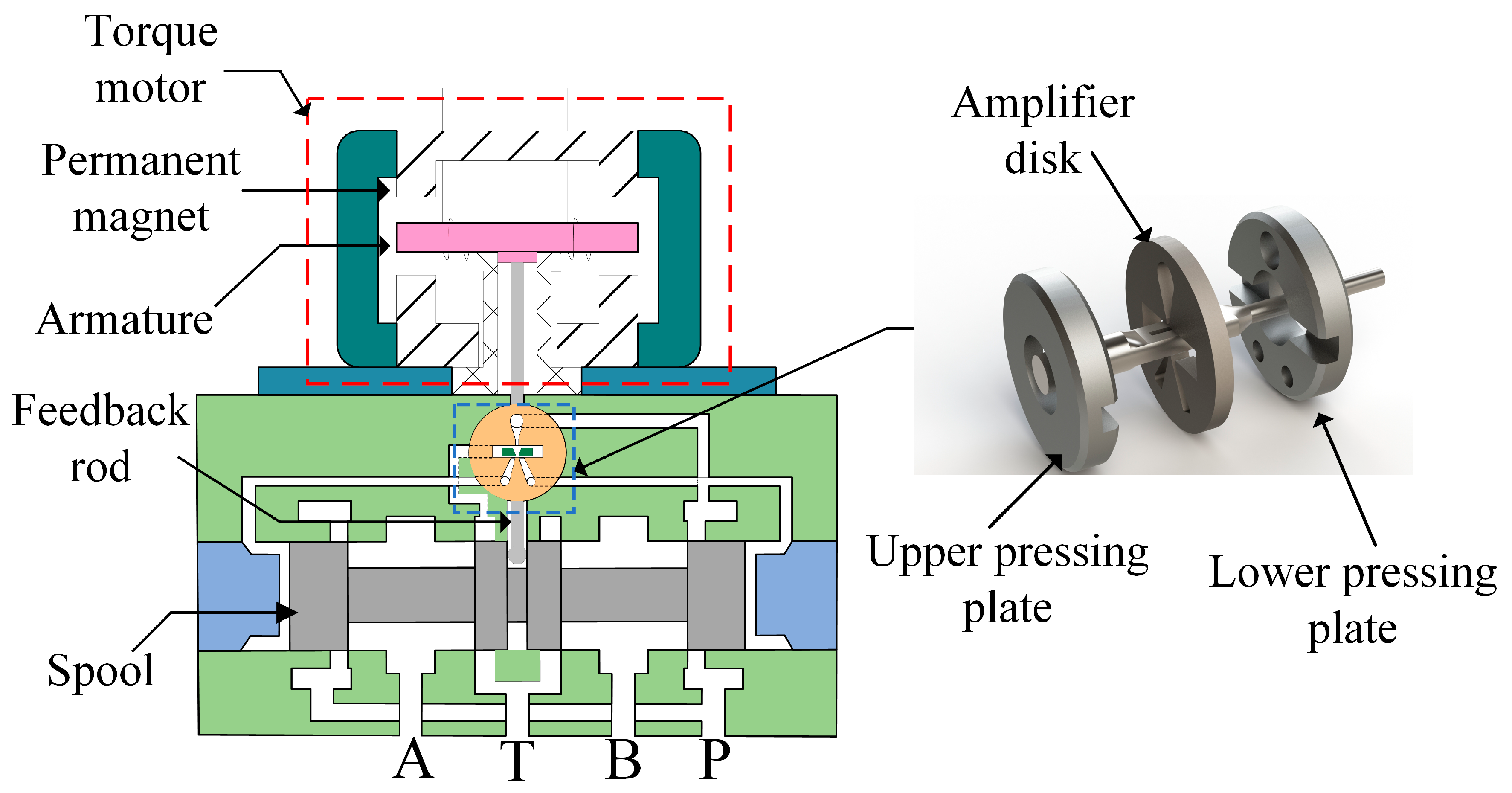
2. The Flow Field of the Pilot Stage

The DJSV is a typical pilot stage servo valve. The pilot stage mainly comprises an electromagnet, deflector plate, jet amplifier, and feedback rod. Its working principle is illustrated in Figure 1. High-pressure oil enters the jet amplifier and is deflected by the flapper into the left and right receiving chambers, where its kinetic energy is converted into pressure energy. An oil path at the bottom of the receiving chambers is connected to the spool; the spool moves left and right under the pressure difference. The spool is mechanically linked to a feedback rod, which is coupled to the electromagnet, forming a closed-loop control system. In the absence of a current, the deflector plate remains centred, and the oil momentum entering both receiving ports is equal; thus, the pressure at both ends is equal, and the spool is in the null position. When a current is applied, assuming that the electromagnet is deflected to the right, the electromagnet drives the deflector to the right. Hence, the oil momentum in the right receiving port is greater than the left, resulting in the pressure on the right side being higher than the left. Thus, the spool moves to the left, pressure port P connects to port A, and tank port T connects to port B. At the same time, the feedback rod is deformed. The deformed feedback rod generates feedback force and acts on the electromagnet. Until the feedback force is equal to the electromagnetic force, the spool will stop moving and remain in its current position. As the current disappears, the spool returns to the null position, closing the ports and isolating P from A and T from B.

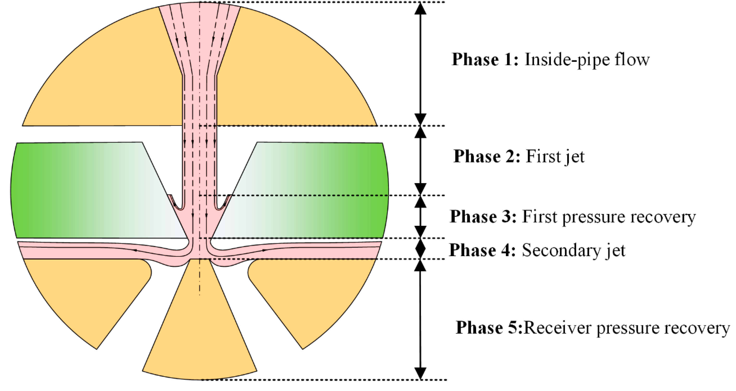
2.1. Flow Field Division

The jet amplifier is a crucial part of the pilot stage and influences the pressure characteristics. The structure of the jet amplifier is shown in Figure 2, and the structural parameters are shown in

Table 1. Parameters of the amplifier.

Parameter	Valve
$\mathrm{Thickness}\mathrm{of}\mathrm{the}\mathrm{jet}\mathrm{pan}{b}_r$	0.54 mm
Thickness of the deflector $D$	0.75 mm
$\mathrm{Distance}\mathrm{from}\mathrm{the}\mathrm{nozzle}\mathrm{outlet}\mathrm{to}\mathrm{the}\mathrm{deflector}\mathrm{top}\mathrm{surface}{L}_j$	0.11 mm
$\mathrm{Width}\mathrm{of}\mathrm{the}\mathrm{outlet}\mathrm{of}\mathrm{the}\mathrm{nozzle}{b}_0$	0.15 mm
$\mathrm{Width}\mathrm{of}\mathrm{the}\mathrm{inlet}\mathrm{of}\mathrm{the}\mathrm{V}-\mathrm{groove}{b}_1$	0.54 mm
$\mathrm{Width}\mathrm{of}\mathrm{the}\mathrm{outlet}\mathrm{of}\mathrm{the}\mathrm{V}-\mathrm{groove}{b}_2$	0.14 mm
$\mathrm{Width}\mathrm{of}\mathrm{the}\mathrm{shunt}\mathrm{wedge}{S}_w$	0.1 mm
$\mathrm{Length}\mathrm{of}\mathrm{the}\mathrm{receiver}{R}_w$	0.17 mm
$\mathrm{Effective}\mathrm{length}\mathrm{of}\mathrm{the}\mathrm{receiver}\mathrm{inlet}{R}_s$	0.15 mm
$\mathrm{Inclination}\mathrm{angle}\mathrm{of}\mathrm{the}\mathrm{inside}\mathrm{pipe}\mathrm{sidewall}{\theta }_i$	13°
$\mathrm{Inclination}\mathrm{angle}\mathrm{of}\mathrm{the}\mathrm{V}-\mathrm{groove}\mathrm{sidewall}{\theta }_d$	17°
$\mathrm{Inclination}\mathrm{angle}\mathrm{of}\mathrm{the}\mathrm{receiver}{\theta }_r$	19°
$\mathrm{Jet}\mathrm{diffusion}\mathrm{angle}{\alpha }_1$	11°
$\mathrm{Jet}\mathrm{core}\mathrm{collection}\mathrm{angle}{\alpha }_2$	5.54°
$\mathrm{Oil}\mathrm{viscosity}\rho$	850 kg/m3
$\mathrm{Oil}\mathrm{density}\mu$	0.0085 N-s/m2

.

In order to facilitate the analysis of the flow field, the pilot stage can be divided into five phases (phase I~V) [25], as shown in Figure 3.

• Phase I: Inside flow phase

The inside flow phase consists of a convergent section and a straight section. When the oil is through the convergent section, the oil velocity increases significantly, and then a stable jet is formed in the straight section and enters the first jet phase.

2.

Phase II: First jet phase

In the first jet phase, the fluid exhibits free jet characteristics, which can be analysed using the free jet theory. This flow region is typically divided into the initial and main jet sections. The initial jet section can be divided into potential core and shear sections. The velocity in the core section is equal everywhere, and the velocity gradient in the shear section is enormous. Due to the interaction between the jet and the surrounding flow, the shear section will diffuse along the jet direction, and the core section will be narrow until it disappears. Then, the jet goes into the main section. The main section has the characteristic of velocity similarity, and the main jet section velocity distribution can be solved based on this theorem.

3.

Phase III: First jet pressure recovery phase

Since the deflector plate is V-shaped and the jet area gradually spreads along the jet direction, the jet will collide with the deflector plate. At the collision point, some parts of the oil will flow out of the V-shaped deflector, and others will continue to flow downward along the groove.

4.

Phase IV: Secondary jet phase

The secondary jet phase, situated at the deflector outlet, exhibits velocity distributions that are strongly influenced by the deflector movement. When the deflector is in the null position, the velocity is symmetrically distributed, and when the deflector shifts, the oil will be affected by the unbalanced force of the V-shaped groove. Hence, the velocity changes to an asymmetrical distribution, affecting the oil momentum in the left and right receiving ports, thus influencing the pilot stage pressure characteristics.

5.

Phase V: Receiver pressure recovery phase

The oil will split into two parts in the receiver pressure recovery phase and enter the left and right receiving ports. Under the pressure model, the receiving port can be considered to be sealed, and the impact of the jet on the oil can be assumed to be the impact of the equivalent piston. The pressure in the receiving port can be obtained by solving the force on the piston.

2.2. Flow Field Assumptions

Since the pilot stage flow situation is complex, to analyse the main factors, it is necessary to make several assumptions [22]:

(I)

The flow field is two-dimensional.

(II)

The oil is incompressible.

(III)

There are no-slip boundary conditions at the walls.

3. Mathematical Model of the Pilot Stage Pressure

Based on the characteristics of the pilot stage flow field, mathematical models are developed for its five phases. (1) In phase 1, the velocity distribution at the nozzle is derived from Bernoulli’s equation; (2) in phase 2, the primary jet region is modelled based on the free jet theory to capture the velocity distribution; (3) in phase 3, the average velocity at the secondary jet outlet is obtained according to the momentum conservation theorem; (4) in phase 4, a dynamic skewed distribution model is employed to describe the velocity distribution under varying deflector displacements; (5) in phase 5, the pressure in the receiving chamber is calculated using the equivalent piston principle. The mathematical models of each region are shown below.

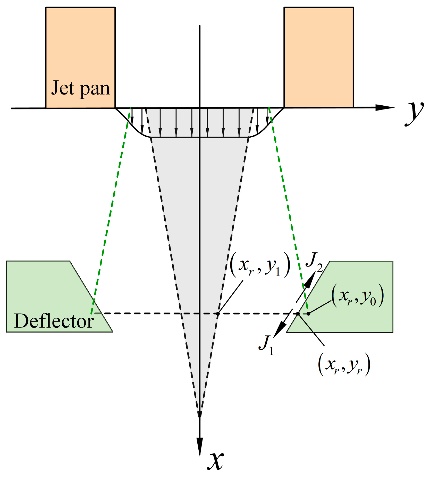
3.1. Velocity Distribution in the Inside Flow Phase

According to the structural characteristics of the pilot stage, energy loss occurs as the oil moves through the convergent section and straight section. Based on the Bernoulli equation, the average velocity at the exit of the nozzle is

$$\begin{array}{c}{\overline{u}}_0=\sqrt{{\displaystyle \frac{2\left(P_s-P_0\right)}{\rho \left(1+{\xi }_P\right)}}}\end{array}$$

(1)

where $P_s$ is the inlet pressure, $P_0$ is the outlet pressure, $\rho$ is the oil density, and ${\xi }_P$ is the energy loss coefficient, which is related to the structure dimensions of the nozzle and the Reynolds number.

The velocity distribution of the fluid is influenced by the flow state and boundary layer effects. When the pilot stage flow is turbulent, transverse fluctuations of fluid micro-elements lead to a more uniform velocity profile across the pipe cross-section. This velocity distribution can be expressed as

$$\begin{array}{c}{u}_0=\sqrt{{\displaystyle \frac{2\left(P_s-P_0\right)}{\rho }}}\end{array}$$

(2)

Owing to the symmetry of the oil velocity profile at the nozzle, this analysis is limited to one side. Within the boundary layer, the velocity follows an exponential distribution [22,26]. Thus, the outlet velocity profile can be expressed as

$$\begin{array}{c}{u}_F=\left\{\begin{array}{c}{u}_0\left(0\le x<b_0/2-\sigma \right)\\ u_0{\eta }_0{e}^{{\displaystyle \frac{1}{k_0}}\left(1-{{\eta }_0}^{k_0}\right)}\left(b_0/2-\sigma \le x\le b_0/2\right)\end{array}\right.\end{array}$$

(3)

where $u_F$ is the nozzle velocity distribution, $u_0$ is the turbulent flat velocity, $\sigma$ is the boundary layer, ${\eta }_0$ is the dimensionless distance from fluid particles within the boundary layer to the wall, ${\eta }_0=\left(b_0/2-x\right)/\sigma$, and $k_0$ is the shape coefficient of the velocity distribution in the boundary layer, which is 0.7.

Based on the average velocity, the momentum passing through the nozzle exit per unit of time can be calculated as follows:

$$\begin{array}{c}{E}_0=\rho {\overline{u}}_0^3{b}_0/2\end{array}$$

(4)

Taking the boundary layer into account, the momentum flux through the nozzle exit per unit time is expressed as

$$\begin{array}{c}{E}_1=\rho {\int }_0^{b_0/2}{u}_F^3\left(x\right)dx\end{array}$$

(5)

Assuming the momentum passing through the nozzle per unit of time remains unchanged regardless of whether the boundary layer is considered, the following relation holds:

$$\begin{array}{c}{E}_0=E_1\end{array}$$

(6)

Substituting Equations (4) and (5) into Equation (6), we get

$$\begin{array}{c}{\overline{u}}_0^3{b}_0/2={\int }_0^{b_0/2}{u}_F^3\left(x\right)\mathrm{d}x\end{array}$$

(7)

Substituting Equation (3) into Equation (7), the boundary layer thickness $\mathrm{\sigma }$ can be given by

$$\begin{array}{c}\sigma =2.342{\displaystyle \frac{\left(u_0^3-{\overline{u}}_0^3\right)}{u_0^3}}{b}_0/2\end{array}$$

(8)

Substituting Equations (1) and (2) into Equation (8), we can have

$$\begin{array}{c}\sigma =2.342\left[1-{\left(1+{\xi }_P\right)}^{-{\displaystyle \frac{3}{2}}}\right]b_0/2\end{array}$$

(9)

By substituting Equation (9) into Equation (3), the nozzle outlet velocity distribution accounting for the boundary layer is obtained.

Figure 4a compares the calculated results under five pressure conditions with and without the boundary layer against CFD simulations. The CFD setup is detailed in Section 4.2 of this paper. The model incorporating the boundary layer shows strong agreement with the CFD results, whereas the uniform model exhibits notable discrepancies. To further assess these differences, Figure 4b presents the velocity deviation between each model and the CFD results. Near the wall, the boundary layer model shows significantly lower deviation compared to the uniform model. Away from the wall, the boundary layer results closely follow the zero-error line, while the uniform model consistently underestimates the velocity. These findings confirm that the boundary layer model provides a more accurate representation of the velocity field across the domain.

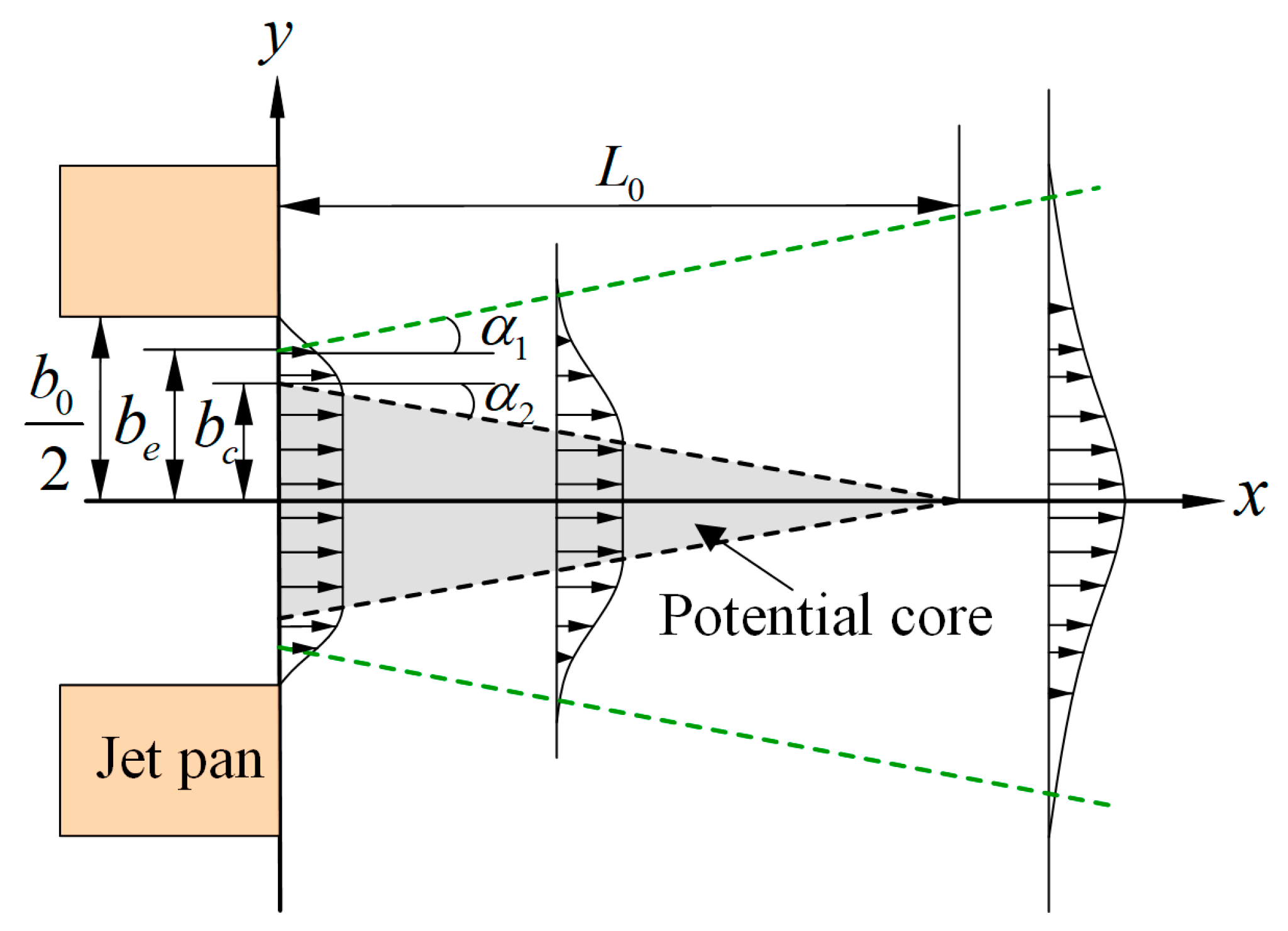
3.2. First Jet Velocity Distribution

The primary jet region can be analysed using the free jet theory, as illustrated in Figure 5. The free jet consists of the potential core and main jet sections. Within the potential core, the velocity remains uniform, and its length is related to the nozzle diameter, given by L₀ = 5.2b₀ [22]. Beyond this region, the jet enters the main section, where the velocity profiles exhibit self-similarity. The velocity distribution in this region can be derived using this theory.

The velocity distribution in the main jet section satisfies in the following form:

$$\begin{array}{c}{\displaystyle \frac{u}{u_{01}}}=\exp \left[-{\left({\displaystyle \frac{y}{b_e}}\right)}^2\right]\end{array}$$

(10)

where $u$ is the velocity distribution of the main section, $u_{01}$ is the axial velocity of the main section, and $b_e$ is the characteristic thickness. The characteristic thickness is usually selected when $u/u_{01}=1/e$. Experiments have found that the characteristic thickness expands linearly along the jet direction, and the relationship is

$$\begin{array}{c}{b}_e=\epsilon x\end{array}$$

(11)

Thus, the velocity distribution can be obtained as

$$\begin{array}{c}u=u_{01}\exp \left[-{\left({\displaystyle \frac{y}{\epsilon x}}\right)}^2\right]\end{array}$$

(12)

The momentum entering the first jet phase is

$$\begin{array}{c}{M}_{00}=2{\int }_0^{b_0}\rho u_F^{2}dy=1.57\rho u_0^2{b}_0\end{array}$$

(13)

The momentum at any cross-section in the main jet section is

$$\begin{array}{c}{M}_{01}={\int }_{-\infty }^{+\infty }\rho u^{2}dy\end{array}$$

(14)

Substituting Equation (12) into (14), we get

$$\begin{array}{c}{M}_{01}=\rho \sqrt{{\displaystyle \frac{\pi }{2}}}{u}_{01}^2\epsilon x\end{array}$$

(15)

According to the law of momentum conservation, the relationship between the velocity of the axis in the main jet section and the velocity in the potential core can be obtained as

$$\begin{array}{c}{\displaystyle \frac{u_{01}}{u_0}}={\left(\sqrt{{\displaystyle \frac{2}{\pi }}}{\displaystyle \frac{1}{\epsilon }}\right)}^{{\displaystyle \frac{1}{2}}}{\left({\displaystyle \frac{1.57b_0}{x}}\right)}^{{\displaystyle \frac{1}{2}}}\end{array}$$

(16)

Since the characteristic thickness expands linearly along the jet direction, the coefficient is $\epsilon =0.348$, so Formula (16) can be simplified to

$$\begin{array}{c}{u}_{01}=1.51{\left({\displaystyle \frac{1.57b_0}{x}}\right)}^{{\displaystyle \frac{1}{2}}}{u}_0\end{array}$$

(17)

Substituting Equation (17) into (12), the velocity distribution in the main jet section is

$$\begin{array}{c}u=1.51{\left({\displaystyle \frac{1.57b_0}{x}}\right)}^{{\displaystyle \frac{1}{2}}}{u}_0\exp \left[-{\left({\displaystyle \frac{y}{0.348x}}\right)}^2\right]\end{array}$$

(18)

3.3. First Jet Pressure Recovery Phase

As the jet area gradually expands along the flow direction while the deflector channel narrows, the oil will collide with the deflector plate at a certain point, denoted as $M_r(x_r,y_r)$. This collision causes a drastic change in the flow field. First, the kinetic energy of the oil will decrease at this point, and the pressure will increase. Second, the impact causes part of the oil to flow back along the wall and eventually flow out of the deflector. The remaining oil will continue to flow downward along the deflector, as shown in Figure 6.

The oil momentum before the collision is $J_0$, the momentum of the oil returning after the collision is $J_2$, and the momentum of the oil continuing to flow downward is $J_1$. According to the law of momentum conservation, we get

$$\begin{array}{c}{J}_{0}cos{\alpha }_1=J_1-J_2\end{array}$$

(19)

$$\begin{array}{c}{J}_0=J_1+J_2\end{array}$$

(20)

$$\begin{array}{c}{J}_0={\displaystyle \frac{M_{01}}{2}}\end{array}$$

(21)

Integrating $J_1$ and $J_2$, we get

$$\begin{array}{c}{J}_1={\int }_0^{y_r}\rho u_{j0}^{2}dy={\int }_0^{y_1}\rho u_0^{2}dy+{\int }_{y_1}^{y_r}\rho u_{j0}^2\exp \left[-{\displaystyle \frac{{\left(y-\left(L_0-x\right)\mathrm{t}\mathrm{a}\mathrm{n}{\alpha }_2\right)}^2}{{\left(b_{ej0}-\left(L_0-x\right)\mathrm{t}\mathrm{a}\mathrm{n}{\alpha }_2\right)}^2}}\right]dy\end{array}$$

(22)

$$\begin{array}{c}{J}_2={\int }_{y_r}^{y_0}\rho u_{j0}^{2}dy={\int }_{y_r}^{y_0}\rho u_0^2\exp \left[-{\displaystyle \frac{{\left(y-\left(L_0-x\right)\mathrm{t}\mathrm{a}\mathrm{n}{\alpha }_2\right)}^2}{{\left(b_{ej0}-\left(L_0-x\right)\mathrm{t}\mathrm{a}\mathrm{n}{\alpha }_2\right)}^2}}\right]dy\end{array}$$

(23)

where $y_0$ is the distance from the jet diffusion zone boundary to the centre and $y_1$ is the distance from the jet core zone boundary to the centre:

$$\begin{array}{c}{y}_0=b_{e0}+x_r\tan {\alpha }_1\end{array}$$

(24)

$$\begin{array}{c}{y}_1=\left(L_0-x_r\right)\tan {\alpha }_2\end{array}$$

(25)

$$\begin{array}{c}{y}_r=-\tan \left(x_r-\left(L_{c1}-L_w\right)\right)+b_1\end{array}$$

(26)

Combining Equations (19)–(26), we can obtain the coordinates of the collision point, $M_r$, $J_1$, and $J_2$.

After passing the collision point, some oil flows toward the deflector outlet. Since this part is still in the deflector, the V-shaped structure will cause local pressure loss. It is assumed that the local pressure loss coefficient is ${\xi }_1^{’}$. According to energy conservation, the average velocity at the outlet of the secondary jet is

$$\begin{array}{c}{\overline{u}}_2=u_0\sqrt[3]{{\displaystyle \frac{1-{\xi }_1^{’}}{b_1}}\left[y_1+{\int }_{y_1}^{y_r}exp\left(-{\displaystyle \frac{3{\left(y-\left(L_{j0}-x_r\right)\mathrm{t}\mathrm{a}\mathrm{n}{\alpha }_1\right)}^2}{{\left(y_0-\left(L_{j0}-x_r\right)\mathrm{t}\mathrm{a}\mathrm{n}{\alpha }_1\right)}^2}}\right)dy\right]}\end{array}$$

(27)

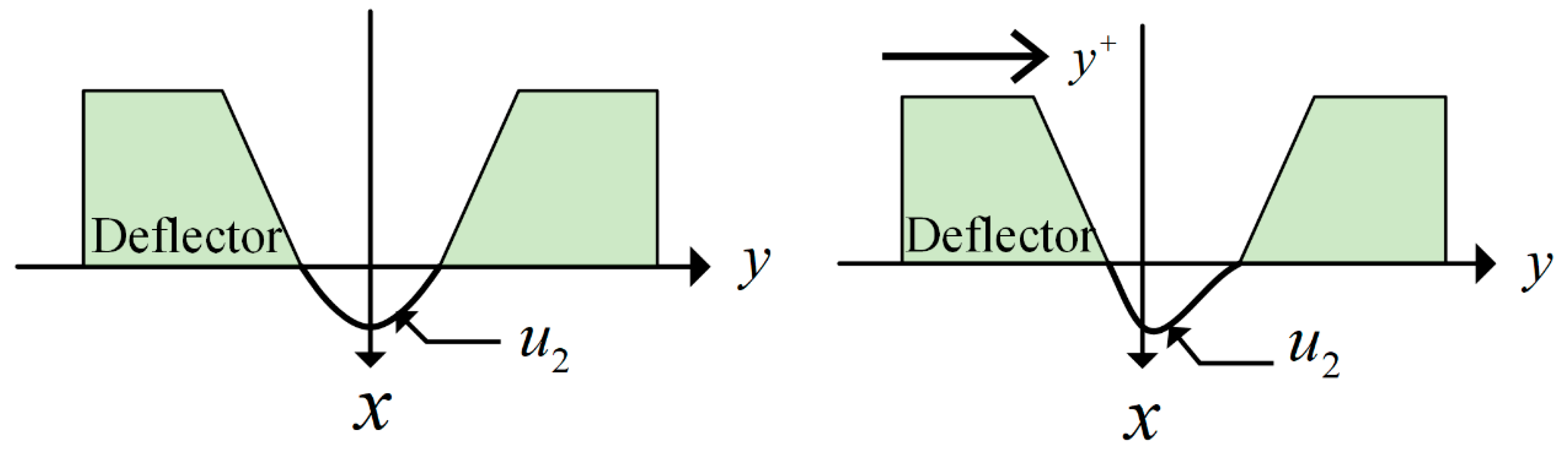
3.4. Secondary Jet Velocity Distribution

The velocity distribution at the deflector outlet is referred to as secondary jet velocity distribution, which directly affects the pressure characteristics of the pilot stage. Studies have shown that this distribution varies with the deflector displacement. When the deflector is in the null position, the velocity distribution is symmetric. As the deflector shifts, the distribution becomes increasingly asymmetric, with greater displacement leading to more pronounced asymmetry. The velocity distribution diagrams are shown in Figure 7.

The secondary velocity distribution is analysed using the skewness function, and the probability density function of the skewed distribution is [27]

$$\begin{array}{c}f\left(x\right)=2\varphi \left(x\right)·\Phi \left(\lambda x\right)\end{array}$$

(28)

where $\lambda$ is the skewness parameter, $\varphi \left(x\right)$ is the standard normal distribution probability density function, and $\Phi \left(x\right)$ is the standard normal distribution function.

The skewness parameter $\lambda$ reflects the skewness. When the skewness parameter is zero, the skewed distribution degenerates to a normal distribution and presents a symmetrical characteristic. When the skewness parameter deviates from zero, the skewed distribution presents an asymmetric characteristic, and the larger the skewness parameter, the more pronounced the asymmetric characteristic. Therefore, the relationship between the displacement and the skewness parameter can be established, and the appropriate $\lambda$ can be selected.

Equation (28) is normalised to obtain the normalised skew distribution function, and we get

$$\begin{array}{c}F\left(x\right)={\displaystyle \frac{f\left(x\right)}{f_{\mathrm{m}\mathrm{a}\mathrm{x}}\left(x\right)}}\end{array}$$

(29)

According to the normalised skew distribution function, the velocity distribution of the secondary jet can be expressed as

$$\begin{array}{c}{u}_2=u_{2\mathrm{m}\mathrm{a}\mathrm{x}}·F\left(x\right)\end{array}$$

(30)

where $u_{2\mathrm{m}\mathrm{a}\mathrm{x}}$ is the maximum velocity at the secondary jet outlet.

Since the maximum velocity at the secondary jet outlet varies with deflector displacements, it must be recalculated for each displacement. Based on Equation (27), the average velocity at the outlet can be determined, and applying the continuity equation, the maximum velocity is given by

$$\begin{array}{c}{\int }_0^{b_2}{u}_{2\mathrm{m}\mathrm{a}\mathrm{x}}·F\left(x\right)dy={\overline{u}}_2·b_2\end{array}$$

(31)

Combining Equations (28)–(31), the secondary velocity distribution can be obtained at each displacement.

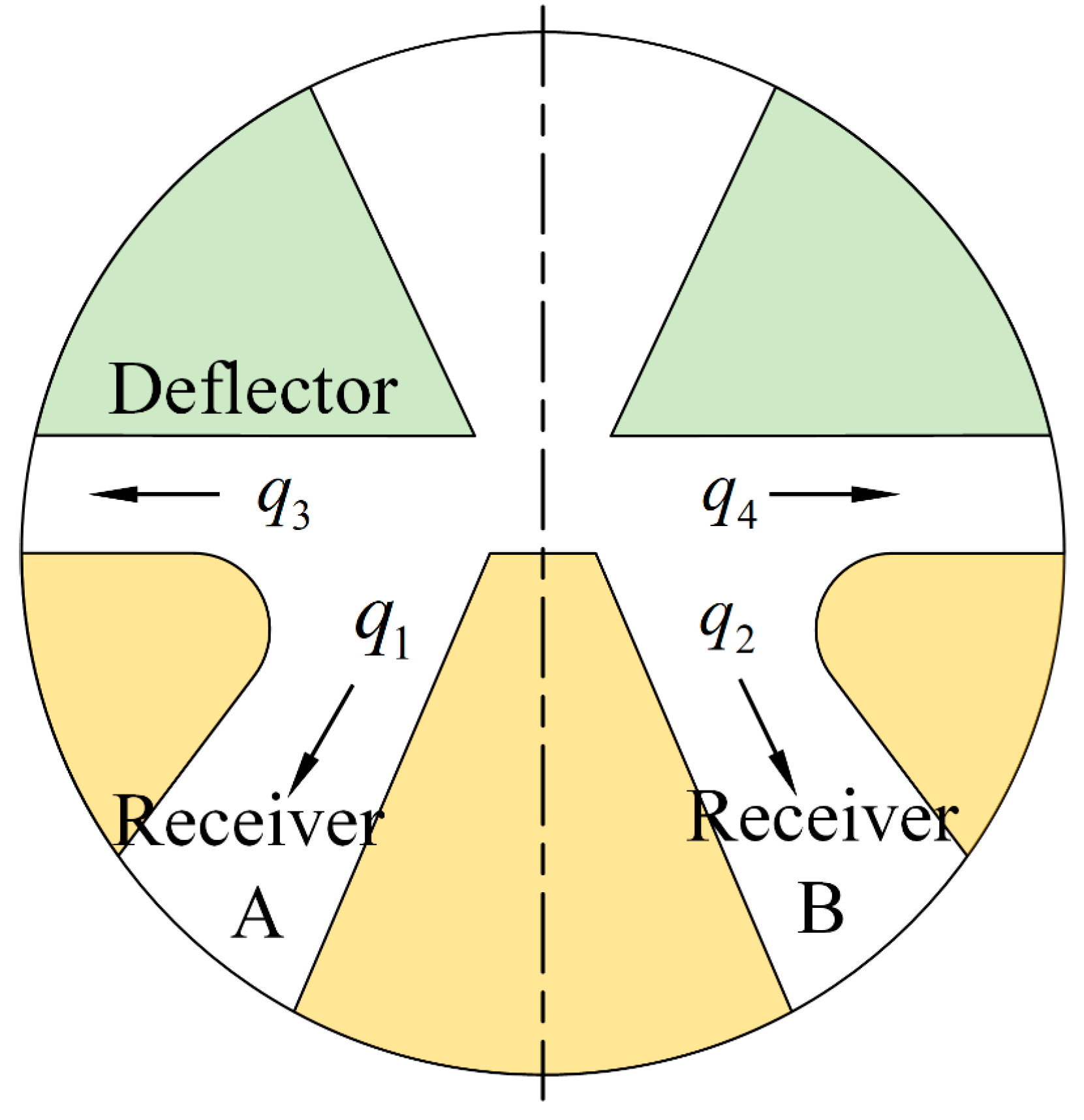
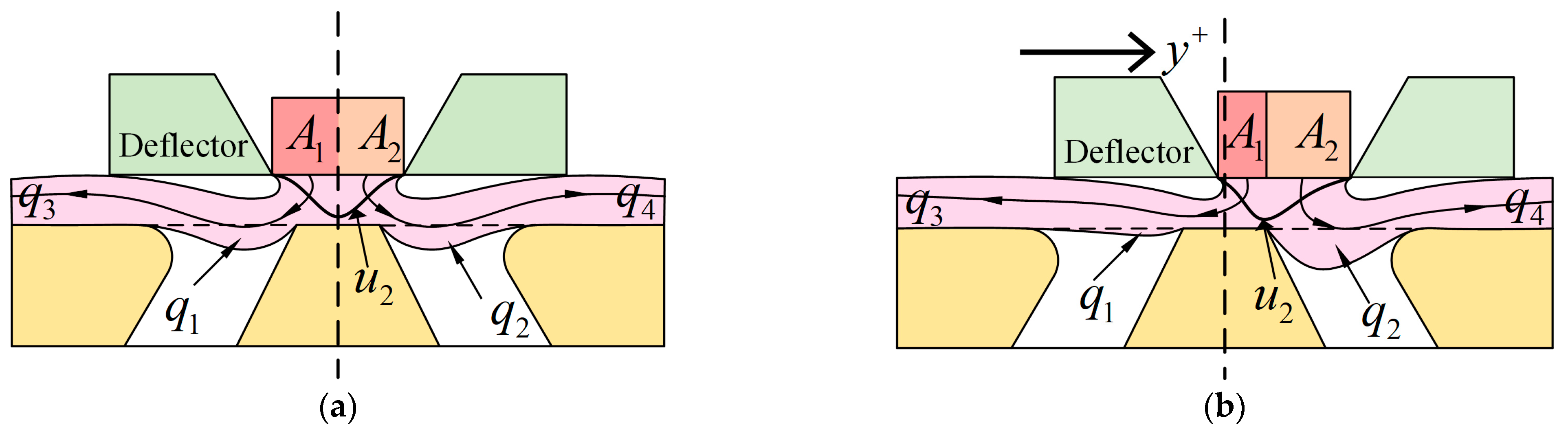
3.5. Receiving Port Pressure Calculation

The receiving port pressure can be calculated using the concept of an equivalent piston theorem, where the jet impact on the fluid is treated as an impact on the non-mass piston. The pressure exerted on the piston surface corresponds to the receiving port pressure. Therefore, it is necessary to calculate the momentum of the fluid entering the receiver. The oil flow at the receiving port is shown in Figure 8.

Due to the collision between the oil and the wedge, part of the oil enters the receiving port at a certain angle, while the remainder exits without entering. In the figure, $q_1$ and $q_2$ represent the oil entering the left and right receivers, and $q_3$ and $q_4$ represent the oil flowing out of the receiving port. When the deflector is in the null position, $q_1$ is equal to $q_2$, and when the deflector is moved, $q_1$ is not equal to $q_2$.

The outlet of the secondary jet is narrow and only slightly larger than the wedge. It is always thought that the outlet of the secondary jet overlaps with the inlet of the receiving port as the effective receiving area. However, when the deflector shifts to the right, the effective receiving area on the left side will inevitably be negative. Negative means the oil collides with the wedge and cannot pass through, resulting in negative pressure in the receiving port, which is inconsistent with the actual situation. This paper uses the secondary outlet area instead of the original receiving area to solve this problem. This approach not only avoids the situation where the receiving area is negative but also reflects the influence of the dynamic distribution of the oil velocity distribution after the deflector moved. This change can effectively improve the calculation accuracy of the receiving port. The influence of the receiving area and the secondary jet velocity distribution are shown in Figure 9.

The receiving area is related to the deflector displacement. When the deflector displacement is zero, the outlet area of the secondary jet is equally divided into the left and right receiving ports. When the deflector is moved, the outlet area is divided into two unequal parts on the left and right, according to the displacement. After the fluid impinges on the splitter tip, the flow direction of the fluid changes, forming angles ${\theta }_1$ and ${\theta }_2$ with the left and right receiving surface, respectively. These angles vary with deflector displacement. Based on this, the flow rates into the left and right receiving ports can be expressed as

$$\begin{array}{c}{q}_1=A_1{u}_{21}\cos {\theta }_1;q_2=A_2{u}_{22}\cos {\theta }_2\end{array}$$

(32)

$$\begin{array}{c}{A}_1=0.5\left(1+{\displaystyle \frac{x_f}{x_{f\mathrm{m}\mathrm{a}\mathrm{x}}}}\right)b_2{b}_r;A_2=0.5\left(1-{\displaystyle \frac{x_f}{x_{f\mathrm{m}\mathrm{a}\mathrm{x}}}}\right)b_2{b}_r\end{array}$$

(33)

where $A_1$ is the left receiving area, $A_2$ is the right receiving area, $u_{21}$ is the velocity distribution of the oil entering the left chamber, $u_{22}$ is the velocity distribution of the oil entering the right chamber, ${\theta }_1$ is the angle between the oil velocity and the left receiving surface, ${\theta }_2$ is the angle between the oil velocity and the right receiving surface, $x_f$ is the deflector displacement, and $x_{f\mathrm{m}\mathrm{a}\mathrm{x}}$ is the maximum displacement. At the maximum displacement, it is assumed that the entire jet enters the corresponding receiving port.

In the receiving port, the kinetic energy of the oil is converted into pressure energy, as shown in Figure 10. The oil mass entering the left receiver per unit time is given by

$$\begin{array}{c}d{m}_1=\rho A_1{u}_{21}\cos {\theta }_{1}dt\end{array}$$

(34)

According to Newton’s second law, the force acting on the piston is

$$\begin{array}{c}{F}_A={\displaystyle \frac{d\left(m_1{u}_{21}\mathrm{c}\mathrm{o}\mathrm{s}{\theta }_1\right)}{dt}}=m_1{\displaystyle \frac{d{u}_{21}\mathrm{c}\mathrm{o}\mathrm{s}{\theta }_1}{dt}}+{\displaystyle \frac{d{m}_1}{dt}}{u}_{21}cos{\theta }_1\end{array}$$

(35)

For steady-state flow, Equation (35) can be simplified as

$$\begin{array}{c}{F}_A={\displaystyle \frac{d\left(m_1{u}_{21}\mathrm{c}\mathrm{o}\mathrm{s}{\theta }_1\right)}{dt}}={\displaystyle \frac{d{m}_1}{dt}}{u}_{21}\mathrm{c}\mathrm{o}\mathrm{s}{\theta }_1\end{array}$$

(36)

Substituting Equation (35) into (36), we can get

$$\begin{array}{c}{F}_A=\rho A_1{\left(u_{21}\mathrm{c}\mathrm{o}\mathrm{s}{\theta }_1\right)}^2\end{array}$$

(37)

Combining Equation (37) with the equivalent piston theorem, the pressure in the left receiving port can be obtained as

$$\begin{array}{c}{P}_A={\displaystyle \frac{F_A}{R_s{b}_r}}{\left(u_{21}\mathrm{c}\mathrm{o}\mathrm{s}{\theta }_1\right)}^2\end{array}$$

(38)

where $R_s$ is the effective length at the entrance of the receiving cavity and $b_r$ is the thickness of the receiving port.

Similarly, the other side receiver pressure can be obtained as

$$\begin{array}{c}{P}_B={\displaystyle \frac{\rho A_2}{R_s{b}_r}}{\left(u_{22}\mathrm{c}\mathrm{o}\mathrm{s}{\theta }_2\right)}^2\end{array}$$

(39)

The load pressure is

$$\begin{array}{c}{P}_L=P_A-P_B={\displaystyle \frac{\rho }{R_s{b}_r}}\left[A_1{\left(u_{21}\mathrm{c}\mathrm{o}\mathrm{s}{\theta }_1\right)}^2-A_2{\left(u_{22}\mathrm{c}\mathrm{o}\mathrm{s}{\theta }_2\right)}^2\right]\end{array}$$

(40)

The dimensionless load pressure is

$$\begin{array}{c}{P}_L^{’}={\displaystyle \frac{P_L}{P_s}}={\displaystyle \frac{\rho }{{P_{s}R}_s{b}_r}}\left[A_1{\left(u_{21}\mathrm{c}\mathrm{o}\mathrm{s}{\theta }_1\right)}^2-A_2{\left(u_{22}\mathrm{c}\mathrm{o}\mathrm{s}{\theta }_2\right)}^2\right]\end{array}$$

(41)

4. Numerical Simulation and Model Validation

Due to the wide pressure range of the servo valve, five representative pressure levels are selected to evaluate the pressure characteristics of the pilot stage, which are 7, 14, 21, 28, and 35 MPa. To assess the improvement by the dynamic skewed model, its results are compared with those obtained from the conventional uniform and normal distribution models. The differences among the three models are analysed, followed by validation using CFD simulations.

4.1. Mathematical Model Calculation

Based on the mathematical models presented in Section 3, the computational procedure for the pilot stage pressure model is illustrated in Figure 11. While the procedures for the uniform and normal distribution models are similar, the key distinction lies in the velocity distribution at the deflector outlet. The dynamic skew model adopts a skewed distribution whose asymmetry varies with deflector displacement. In contrast, the uniform and normal models assume fixed velocity profiles that do not vary with displacement.

As the outlet velocity distribution is symmetric for both left and right deflector displacements, analysing displacement on one side suffices to characterise its behaviour. Based on the above calculations, the velocity distributions at the deflector outlet for the three models are show in Figure 12.

Figure 12a–e show the velocity distributions at the deflector outlet under different displacements for pressures from 7 MPa to 35 MPa. The uniform and normal distribution models exhibit constant, symmetric velocity profiles regardless of displacement. Conversely, the dynamic skew model displays significant asymmetry that increases with deflector displacement. Figure 12f illustrates the skewness coefficient variation across pressures and displacements, revealing that skewness is nearly identical at different pressures for the same displacement and rises with increasing displacement.

4.2. Numerical Simulation

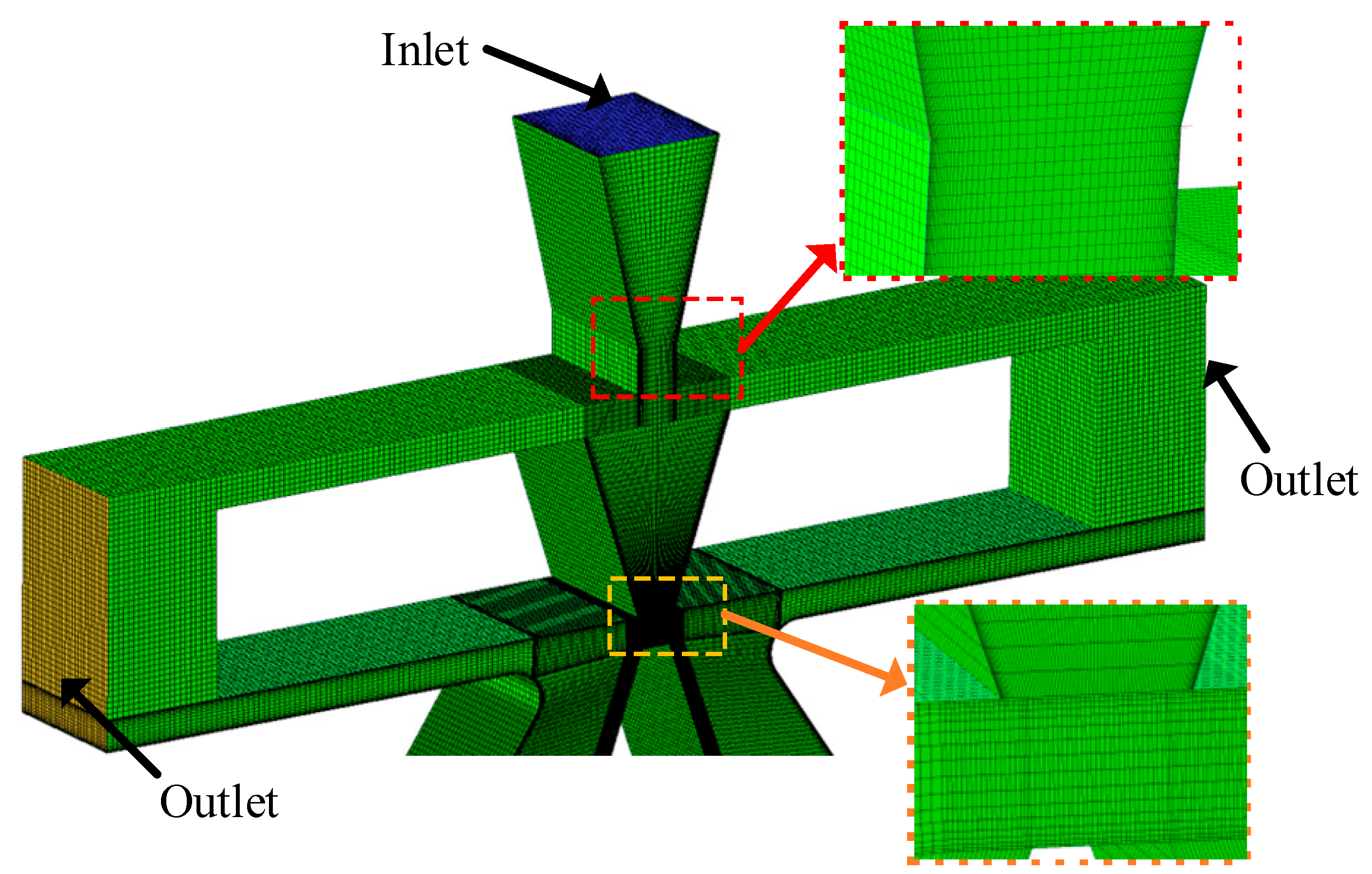
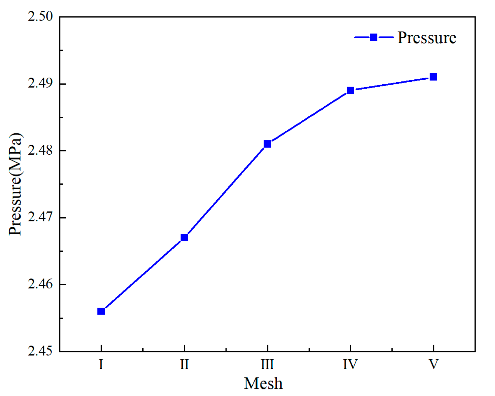
4.2.1. Flow Domain and Mesh Independence Test

The development of computational fluid dynamics has made flow analysis more scientific and efficient. The process generally involves creating a finite element model, setting boundary conditions, and selecting an appropriate solver. In this study, ICEM software (2022 R2) was employed to generate a fully hexahedral mesh, improving computational accuracy and efficiency [28]. To capture boundary layer effects, mesh refinement was applied near the walls, and the finite element mesh is illustrated in Figure 13.

The number of meshes also affects the accuracy of the results. Too few meshes will lead to rough results and a loss of considerable flow information, while too many meshes will significantly increase the calculation time, but the accuracy of the results will not improve. Hence, choosing an appropriate mesh is essential. A mesh independence study was conducted using receiver chamber pressure as the evaluation metric. Five mesh configurations were tested, as detailed in

Table 2. Mesh number and receiver chamber pressure.

Mesh	Number of Cells	Number of Mesh	Pressure (MPa)
Mesh I	1,458,106	1,376,955	2.456
Mesh II	1,825,374	1,730,680	2.467
Mesh III	2,279,004	2,168,576	2.481
Mesh IV	2,922,988	2,791,800	2.489
Mesh V	3,772,624	3,616,614	2.491

, and the corresponding pressure results are illustrated in Figure 14.

Figure 14 shows that the receiver chamber pressure increases with the number of cells before mesh IV, and the pressure changes slightly with the increase in the number of cells after mesh IV. The result indicates that mesh IV is suitable for this simulation.

4.2.2. Boundary Condition

The computational model employs three boundary conditions: inlet, outlet, and wall. The inlet is specified as a pressure inlet, with five representative pressure levels, which are 7 MPa, 14 MPa, 21 MPa, 28 MPa, and 35 MPa, selected to reflect the full operating range of the servo valve. The outlet is defined as a pressure outlet with a fixed value of 0.5 MPa. Wall boundaries are modelled using a no-slip condition to accurately capture near-wall flow behaviour. A low Reynolds number turbulence model is adopted to account for transitional and viscous effects, and the SIMPLE algorithm is used for pressure–velocity coupling [29,30]. The working fluid is specified as No. 10 aviation hydraulic oil, with a density of 850 kg/m³ and a dynamic viscosity of 0.0085 N·s/m². The deflector plate displacement ranges from −0.06 mm to +0.06 mm, with an increment of 0.01 mm, allowing detailed resolution of the flow field response to varying deflector plate positions.

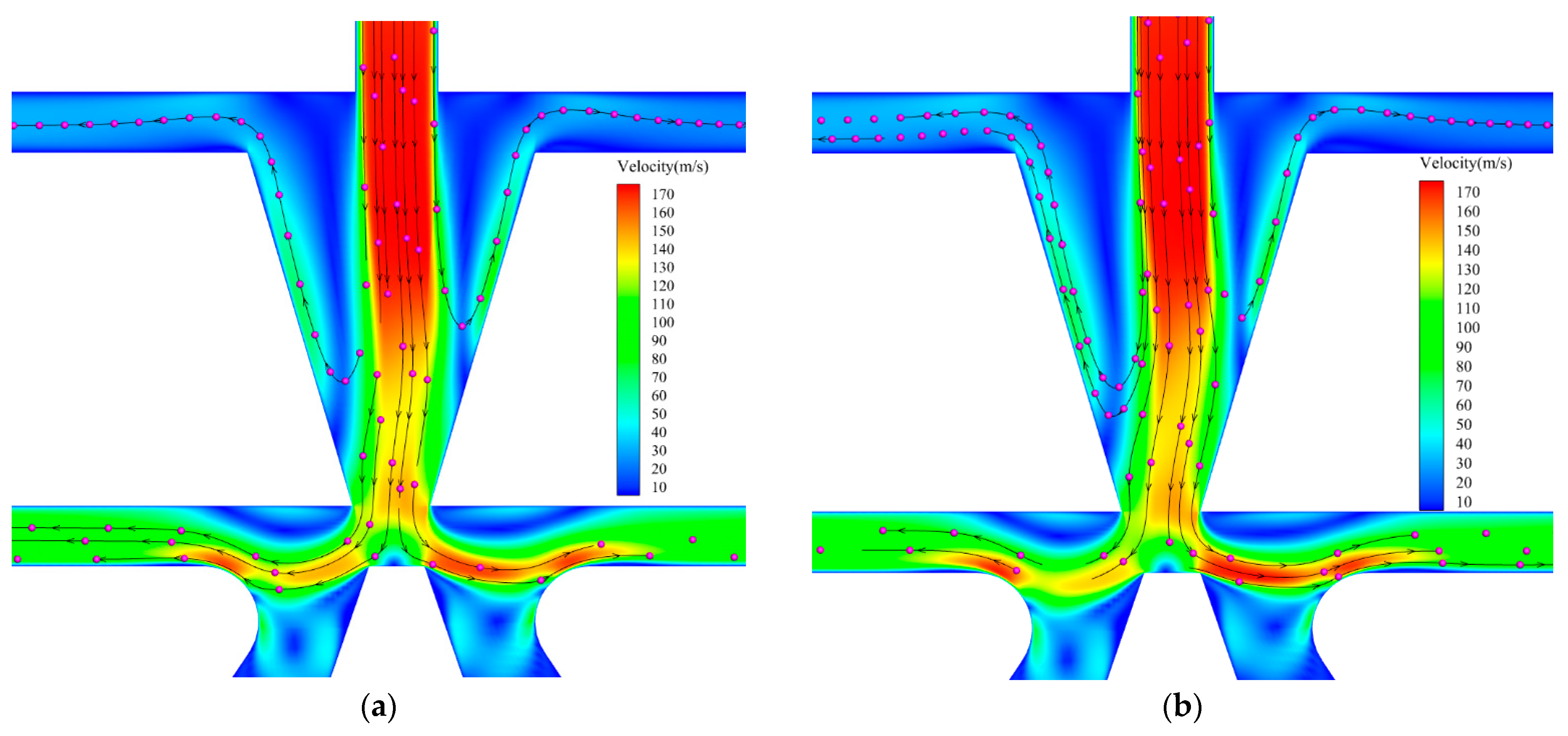
4.2.3. CFD Simulation Results

The CFD results clearly illustrate the flow behaviour within the pilot stage. Figure 15 presents the flow field at an inlet pressure of 14 MPa with leftward deflection. The oil impacts the deflector wall, causing partial backflow, while the remaining flow exits through the outlet.

The exiting jet then strikes the wedge tip and divides into two streams, entering the left and right receiving chambers. The deflector displacement alters the velocity distribution at the secondary jet outlet, thereby affecting the momentum entering each chamber. Figure 15a–f shows the flow evolution as the deflection increases from 0.01 mm to 0.06 mm. The results reveal increasing asymmetry in the velocity distribution with greater displacement, indicating that deflector displacement significantly influences jet skewness and flow division.

4.3. Results and Discussion

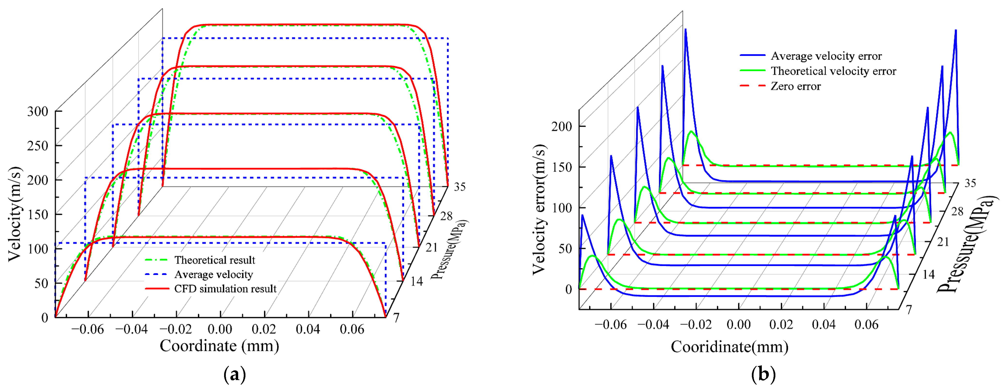
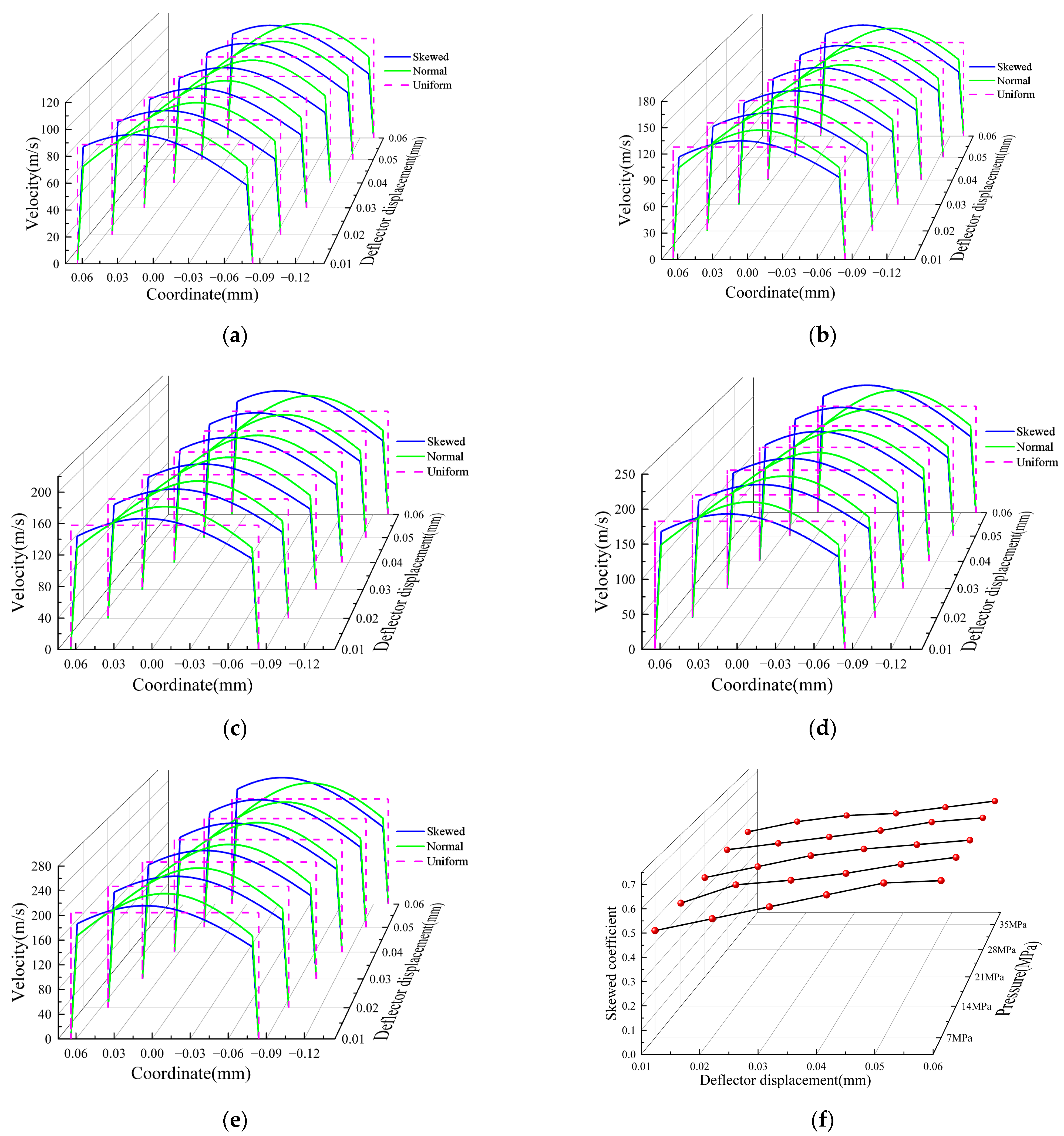
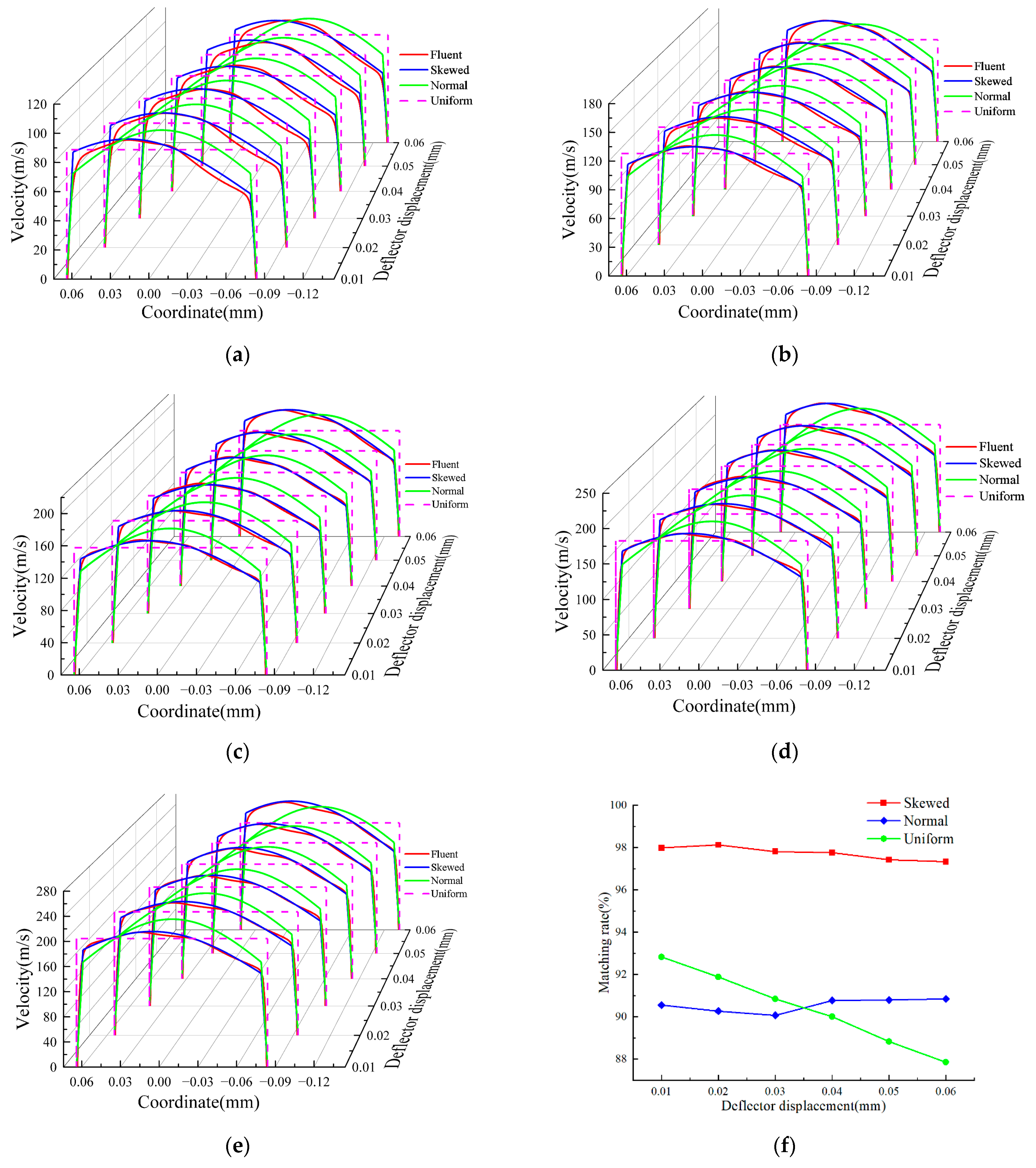
4.3.1. Comparison of Secondary Jet Velocity Distribution

To validate the accuracy of the dynamic skew model, its results are compared against those derived from normal and uniform distributions, as well as Fluent simulations. The differences and underlying causes among the three velocity profiles are analysed. Figure 16 presents the comparison under various pressure conditions.

Fluent simulations indicate that when the deflector shifts leftward, the velocity distribution becomes distinctly asymmetric across all pressure levels, with the peak velocity of the secondary jet shifting to the right, as shown in Figure 16a–e. The dynamic skew distribution model demonstrates strong agreement with the Fluent results, indicating its capability to accurately capture the velocity distribution characteristics during deflector displacement. In contrast, the uniform and normal distribution models fail to reflect this asymmetry and thus are inadequate in representing the true behaviour of the secondary jet flow.

To quantitatively evaluate the deviation between each velocity distribution model and the Fluent results, matching rates were used, as shown in Figure 16f. The dynamic skew velocity matching rate achieved a conformity rate of 98% across all displacements. The normal distribution showed lower accuracy, with 90% at small displacements to 91% at larger ones. The uniform distribution performed worst, with conformity decreasing from 93% at 0.01 mm to 88% at 0.06 mm. This trend confirms that velocity asymmetry increases with deflector displacement, aligning with the growing skewness in the dynamic model. Overall, the dynamic skew distribution more accurately captures the secondary jet characteristics than the uniform and normal models.

The velocity distribution is governed by the combined effects of the pilot stage geometry and deflector displacement, fundamentally linked to the force balance on fluid micro-elements. In channel flow, viscous forces dominate near the wall, while inertial forces dominate away from it [31], resulting in a symmetric trapezoidal profile under parallel boundaries. However, the V-shaped narrowing of the deflector induces transverse velocities in the flow. When the deflector is in the null position, the jet symmetrically interacts with both walls, producing a symmetric velocity distribution. With leftward deflection, the jet first contacts the right wall, generating a greater transverse velocity and velocity gradient on that side. This leads to an asymmetric velocity profile, which becomes more pronounced as the deflection increases, reflecting stronger disparities in velocity gradients across the channel.

The normal distribution is symmetric, with a peak at the centre and lower values on both sides, and remains unchanged with deflector displacement. At small displacements, the velocity distribution exhibits low skewness and a relatively flat profile. With displacement increases, the skewness becomes more evident, shifting the peak velocity position. This shift leads to a slightly higher fit rate under larger displacements compared to smaller ones.

In the uniform distribution model, the secondary jet velocity is assumed constant across the outlet and independent of deflector displacement. In practice, however, velocity skewness increases with displacement, leading to a growing mismatch between the uniform and actual distributions. As a result, the matching rate of the uniform model decreases with increasing deflector displacement.

The preceding analysis confirms that the dynamic skewed distribution accurately characterises the variation in secondary jet velocity profiles, outperforming both the normal and uniform distribution models.

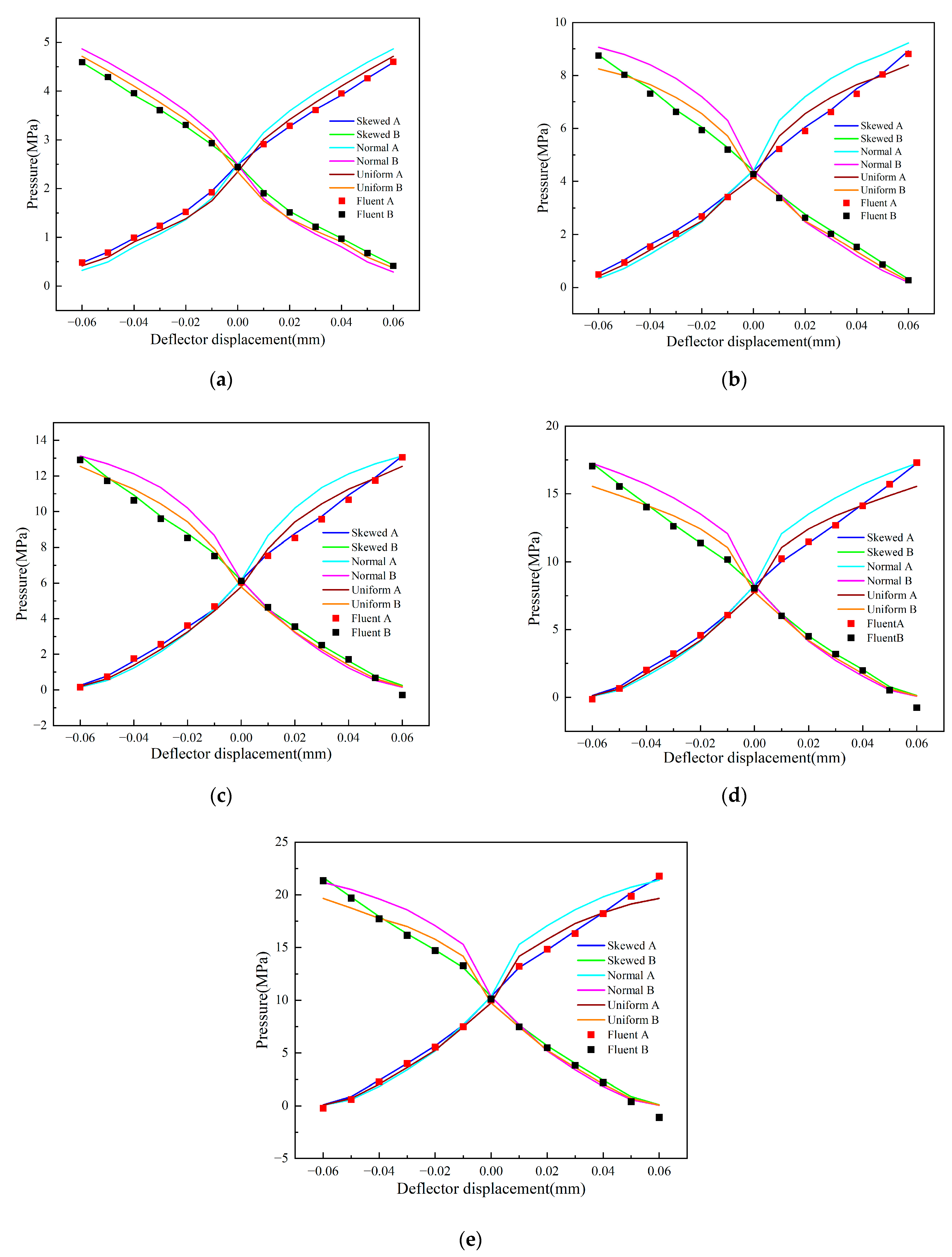
4.3.2. Comparison of Pressure Model Results

As previously discussed, the displacement of the deflector alters the velocity distribution at the outlet, which in turn affects the momentum of the fluid entering the receiving chambers, leading to variations in chamber pressure. To quantify this effect, the pressure results under three different velocity distributions are compared with those obtained from the Fluent simulations. The pressure characteristics at various inlet pressures are analysed, as illustrated in Figure 17, where A and B represent the left and right receiving chambers, respectively.

Given the symmetry in the pressure variation of the left and right receiving chambers regardless of the deflector’s displacement direction, the analysis focuses on the case where the deflector is displaced to the left. Figure 17a shows that at an inlet pressure of 7 MPa, the pressure predicted using the normal distribution is highest, followed by the uniform and then the skewed distribution. The differences between them remain nearly constant across varying deflection distances.

At higher inlet pressures, the normal distribution continues to yield the highest pressure. However, the difference between the normal and skewed distributions first increases and then decreases with larger deflection distances. In contrast, for the uniform and skewed distributions, the uniform model predicts higher pressure at small deflections, while the skewed model surpasses it at larger deflections. Thus, the difference between these two distributions first decreases and then increases with deflection distance, as illustrated in Figure 17b–e. Among the three velocity distributions, only the skewed distribution produces a pressure curve that closely matches the Fluent simulation results.

The pressure in the right receiving chamber show that the skewed velocity distribution yields slightly higher values than the uniform and normal distributions, which exhibit minimal difference. The skewed distribution also shows the best agreement with the Fluent simulations.

Bernoulli’s principle indicates that kinetic energy of the fluid within the receiving chambers is converted into pressure energy, with the former governed by the velocity distribution at the deflector outlet. When the deflector is shifted to the left, the skewed velocity distribution results in a higher peak velocity on the right side, leading to a greater average inflow velocity into the right chamber. This asymmetry varies dynamically with deflector displacement. For a normal distribution, the velocity profile is symmetric, with average velocities in both chambers varying with displacement. In contrast, a uniform distribution assumes constant velocity across the outlet, resulting in equal average velocities into both chambers, regardless of deflector position.

The comparison of the skewed and normal distributions shows that, at small deflections, the skewed distribution has a lower skewness coefficient, resulting in a lower average velocity than the normal distribution. As deflection increases, the average velocity of the skewed distribution increases, while that of the normal distribution decreases, leading to a gradual reduction in the pressure difference between them. Similarly, compared with the uniform distribution, the skewed distribution initially produces a lower average velocity. However, with increasing deflection, its average velocity surpasses that of the uniform distribution. Therefore, the skewed distribution yields lower pressure at small deflections but higher pressure at larger deflections.

The analysis of the right receiving chamber indicates that the average velocity under the skewed distribution marginally exceeds that of the normal and uniform distributions, resulting in correspondingly higher pressure. This similarly accounts for the pressure characteristics when the deflector shifts right.

To further compare the pressure characteristics of the three velocity distributions in the pilot stage, their dimensionless load pressures were calculated and compared with the Fluent results, as shown in Figure 18. The results indicate that the skewed distribution aligns most closely with the Fluent data, while the uniform and normal distributions exhibit significant deviations. The maximum errors for the skewed, normal, and uniform distributions are 1.43%, 9.52%, and 8.10%, respectively. The skewed model improves accuracy by 84.98% and 82.35% compared to the normal and uniform models. These results confirm that the skewed distribution provides a more accurate and robust representation of pressure characteristics than conventional models.

5. Conclusions

This study investigates the influence of velocity distribution on the pressure characteristics of the pilot stage. A mathematical model of pilot stage pressure under a dynamically skewed velocity distribution was developed and compared with normal and uniform distributions, as well as CFD simulation results. The velocity profile of the secondary jet and corresponding pressure behaviour were analysed in detail. The main conclusions are as follows:

• The secondary jet velocity distribution changes with the deflector displacement. The skewed distribution effectively represents this variation. At the null position, the outlet velocity resembles a normal distribution. With increasing deflector displacement, the distribution becomes increasingly asymmetric, reflected by a rising skewness coefficient.
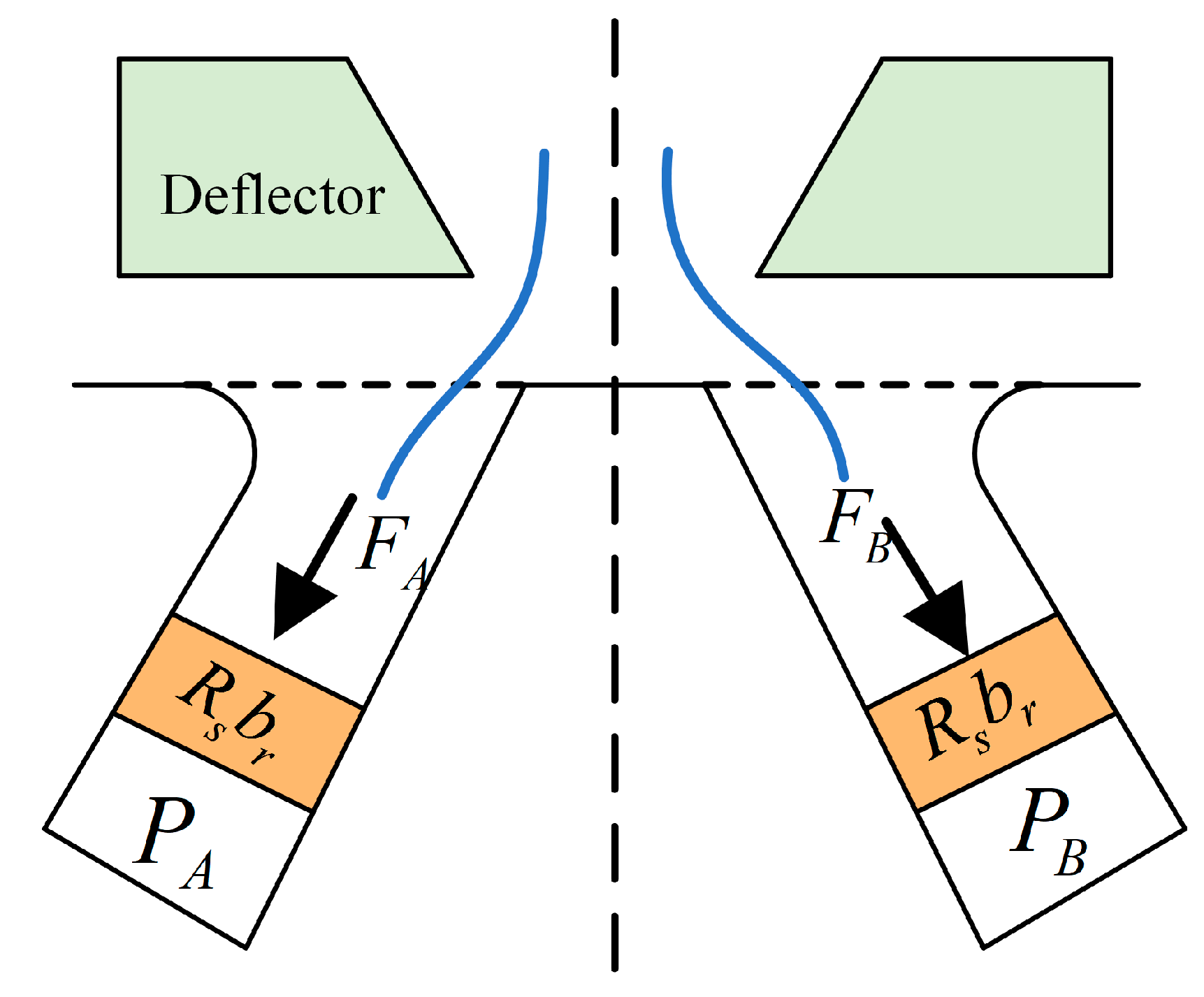
• The pressure within the receiving chambers is affected both by their receiving areas and the velocity distribution of the secondary jet. Deflector displacement alters the velocity distribution result in the differing fluid momentum entering the left and right chambers. The chamber with the smaller receiving area experiences a higher jet velocity than the one with the larger area.
• Substituting the original receiving area with the secondary jet outlet area prevents negative effective areas, aligning the results more closely with actual conditions. This method also captures the effect of velocity distribution on receiver chamber pressure, providing deeper insight into pilot stage flow characteristics.
• The dynamic skewed distribution model precisely represents the secondary jet velocity profile and pilot stage pressure characteristics, demonstrating superior accuracy compared to traditional normal and uniform distribution models.

This study offers a comprehensive analysis of the pilot stage flow in a deflector jet servo valve, addressing the issue of significant deviations in pressure characteristics. The findings offer a theoretical foundation for the development, performance prediction, and structural optimisation of high-performance servo valves and contribute to potential strategies for mitigating pressure fluctuations, cavitation, and related issues.

References

1. Tamburrano, P.; Plummer, A.R.; Distaso, E.; Amirante, R. A review of electro-hydraulic servovalve research and development. Int. J. Fluid Power 2018, 20, 1–23. [Google Scholar] [CrossRef]
2. Wang, Y.; Yin, Y. Performance reliability of jet pipe servo valve under random vibration environment. Mechatronics 2019, 64, 102286. [Google Scholar] [CrossRef]
3. Xu, B.; Shen, J.; Liu, S.; Su, Q.; Zhang, J. Research and Development of Electro-hydraulic Control Valves Oriented to Industry 4.0: A Review. Chin. J. Mech. Eng. 2020, 33, 29. [Google Scholar] [CrossRef]
4. Zhang, L.; Huang, Z.; Fu, C.; Xu, Y.; Wang, Y.; Kong, X. Design and Verification of Two-Stage Brake Pressure Servo Valve for Aircraft Brake System. Processes 2021, 9, 979. [Google Scholar] [CrossRef]
5. Yang, H.; Wang, W.; Lu, K. Cavitation and flow forces in the flapper-nozzle stage of a hydraulic servo-valve manipulated by continuous minijets. Adv. Mech. Eng. 2019, 11, 1687814019851436. [Google Scholar] [CrossRef]
6. Ma, L.; Yan, H.; Ren, Y.; Li, L.; Cai, C. Numerical Investigation of Flow Force and Cavitation Phenomenon in the Pilot Stage of Electrical-Hydraulic Servo Valve under Temperature Shock. Machines 2022, 10, 423. [Google Scholar] [CrossRef]
7. Saha, B.K.; Peng, J.; Li, S. Numerical and Experimental Investigations of Cavitation Phenomena Inside the Pilot Stage of the Deflector Jet Servo-Valve. IEEE Access 2020, 8, 64238–64249. [Google Scholar] [CrossRef]
8. Ren, Y.; Yan, H.; Cai, C. Numerical Study on Flow-Induced Noise of Deflector Jet Servo Valve Based on LES/Lighthill Hybrid Method. Shock Vib. 2022, 2022, 8379245. [Google Scholar] [CrossRef]
9. Hang, J.; Li, Y.; Yang, L. A novel low pressure-difference fluctuation electro-hydraulic large flowrate control valve for fuel flowrate control of aeroengine afterburner system. Chin. J. Aeronaut. 2022, 35, 363–376. [Google Scholar] [CrossRef]
10. Abdallah, H.K.; Peng, J.; Li, S. Analysis of pressure oscillation and structural parameters on the performance of deflector jet servo valve. Alex. Eng. J. 2023, 63, 675–692. [Google Scholar] [CrossRef]
11. Chen, M.; Aung, N.Z.; Li, S.; Zou, C. Effect of Oil Viscosity on Self-Excited Noise Production Inside the Pilot Stage of a Two-Stage Electrohydraulic Servovalve. J. Fluids Eng. 2018, 141, 011106. [Google Scholar] [CrossRef]
12. Yan, H.; Li, J.; Cai, C.; Ren, Y. Numerical Investigation of Erosion Wear in the Hydraulic Amplifier of the Deflector Jet Servo Valve. Appl. Sci. 2020, 10, 1299. [Google Scholar] [CrossRef]
13. Liang, N.; Yuan, Z.; Zhang, F. Oil Particle-Induced Erosion Wear on the Deflector Jet Servo Valve Prestage. Aerospace 2023, 10, 67. [Google Scholar] [CrossRef]
14. Chu, Y.; Yuan, Z.; He, X.; Dong, Z. Model Construction and Performance Degradation Characteristics of a Deflector Jet Pressure Servo Valve under the Condition of Oil Contamination. Int. J. Aerosp. Eng. 2021, 2021, 8840084. [Google Scholar] [CrossRef]
15. Kang, S.; Kong, X.; Zhang, J.; Du, R. Research on Pressure-Flow Characteristics of Pilot Stage in Jet Pipe Servo-Valve. Sensors 2023, 23, 216. [Google Scholar] [CrossRef] [PubMed]
16. Li, Y. Mathematical modelling and characteristics of the pilot valve applied to a jet-pipe/deflector-jet servovalve. Sens. Actuators A Phys. 2016, 245, 150–159. [Google Scholar] [CrossRef]
17. Li, S.L.; Yin, Y.B.; Yuan, J.Y.; Guo, S.R. Three-dimensional flow field mathematical model inside the pilot stage of the deflector jet servo valve. J. Zhejiang Univ.-Sci. A 2022, 23, 795–806. [Google Scholar] [CrossRef]
18. Yan, H.; Bai, L.; Kang, S.; Dong, L.; Li, C. Theoretical model and characteristics analysis of deflector-jet servo valve’s pilot stage. J. Vibroeng. 2017, 19, 4655–4670. [Google Scholar] [CrossRef]
19. Yan, H.; Wang, F.J.; Li, C.C.; Huang, J. Research on the jet characteristics of the deflector–jet mechanism of the servo valve. Chin. Phys. B 2017, 26, 256–264. [Google Scholar] [CrossRef]
20. Liu, X.; Yin, Y.; Wang, Y.; Wang, W.; Wang, X.; Wang, H. The flow field modeling and performance analysis method for the pilot stage of deflector jet servo valve. Flow Meas. Instrum. 2025, 103, 102851. [Google Scholar] [CrossRef]
21. Saha, B.K.; Li, S.; Lv, X. Analysis of pressure characteristics under laminar and turbulent flow states inside the pilot stage of a deflection flapper servo-valve: Mathematical modeling with CFD study and experimental validation. Chin. J. Aeronaut. 2020, 33, 1107–1118. [Google Scholar] [CrossRef]
22. Chen, Z.; Ge, S.; Jiang, Y.; Lin, W.; Zhu, Y. Mathematical modeling of pressure characteristics of the deflector-jet pilot stage considering boundary layer flow. Flow Meas. Instrum. 2023, 90, 102312. [Google Scholar] [CrossRef]
23. Beltaos, S.; Rajaratnam, N. Impingement of axisymmetric developing jets. J. Hydraul. Res. 1977, 15, 311–326. [Google Scholar] [CrossRef]
24. Yan, H.; Mao, Q.; Ren, Y.; Yao, L. Mechanism Analysis of the Secondary Jet of Jet Deflector Servo Valve. In Proceedings of the 2019 IEEE 8th International Conference on Fluid Power and Mechatronics (FPM), Wuhan, China, 10–13 April 2019; pp. 826–832. [Google Scholar]
25. Yan, H.; Ren, Y.; Yao, L.; Dong, L. Analysis of the Internal Characteristics of a Deflector Jet Servo Valve. Chin. J. Mech. Eng. 2019, 32, 31. [Google Scholar] [CrossRef]
26. Tang, S.-J.; LI, M.-J. An Optimum Approximate Analytical Solution for Laminarboundary Layer Velocity with Flat Distribution. J. Xiangtan Univ. (Nat. Sci. Ed.) 2013, 35, 18–20. [Google Scholar]
27. Azzalini, A. A class of distributions which includes the normal ones. Scand. J. Stat. 1985, 12, 171–178. [Google Scholar]
28. Katz, A.; Sankaran, V. Mesh quality effects on the accuracy of CFD solutions on unstructured meshes. J. Comput. Phys. 2011, 230, 7670–7686. [Google Scholar] [CrossRef]
29. Jones, W.P.; Launder, B.E. The calculation of low-Reynolds-number phenomena with a two-equation model of turbulence. Int. J. Heat Mass Transf. 1973, 16, 1119–1130. [Google Scholar] [CrossRef]
30. Ren, Y.; Yan, H.; Bai, L.; Zhang, Y.; Li, C. Simulation on Flow Field Characteristics of Deflector Jet Servo Valve Pre-Stage Under Different Turbulence Models. J. Beijing Jiaotong Univ. 2018, 42, 127–133+140. [Google Scholar]
31. Li, Z.; He, L.; Zhou, J.; Zuo, Y.; Yin, Y.; Zhang, P.; Meng, B. Numerical study on influence of protrusion heights on Reynolds stress and viscous stress variations in turbulent vortical structures. Chin. J. Aeronaut. 2024, 37, 59–71. [Google Scholar] [CrossRef]
Figure 1. Internal structure of the DJSV.
Aerospace 12 00638 g001
Figure 2. The jet amplifier structure.
Aerospace 12 00638 g002
Figure 3. Division of the flow process with the pilot stage.
Aerospace 12 00638 g003
Figure 4. Flow velocity distribution at the nozzle. (a) Five types pressure velocity distribution; (b) Five types pressure Velocity distribution error.
Aerospace 12 00638 g004
Figure 5. Velocity distribution at the first jet phase.
Aerospace 12 00638 g005
Figure 6. Deflector pressure recovery phase.
Aerospace 12 00638 g006
Figure 7. Velocity distribution at the secondary jet.
Aerospace 12 00638 g007
Figure 8. Oil flow in the receiving port.
Aerospace 12 00638 g008
Figure 9. Effective area with zero displacements and moved displacement: (a) null displacement; (b) moved displacement.
Aerospace 12 00638 g009
Figure 10. Receiving port pressure recovery.
Aerospace 12 00638 g010
Figure 11. Calculation process of the pressure characteristics.
Aerospace 12 00638 g011
Figure 12. Comparison of secondary jet velocity distribution under different pressures in three types of mathematical models and skewed coefficient. Subfigures (ae) represent the secondary velocity distribution and the inlet pressures, which are 7 MPa, 14 MPa, 21 MPa, 28 MPa, and 35 MPa, respectively; (f) Skewed coefficient under different inlet pressures and deflector displacements.
Aerospace 12 00638 g012
Figure 13. Meshing model.
Aerospace 12 00638 g013
Figure 14. Relationship between the mesh and the receiver chamber pressure.
Aerospace 12 00638 g014
Figure 15. Velocity distribution under different deflector displacements at 14 MPa. Subfigures (af) represent the deflector displacements, which are 0.01 mm, 0.02 mm, 0.03 mm, 0.04 mm, 0.05 mm, and 0.06 mm respectively.
Aerospace 12 00638 g015aAerospace 12 00638 g015b
Figure 16. Comparison of CFD results and three types of mathematical models on secondary velocity distribution under different pressure and velocity matching rates under different pressures. Subfigures (ae) represent the secondary velocity distributions and the inlet pressures, which are 7 MPa, 14 MPa, 21 MPa, 28 MPa, and 35 MPa, respectively. (f) Three types of velocity matching rates under different displacements.
Aerospace 12 00638 g016
Figure 17. Comparison of CFD results and three types of mathematical models in pilot stage pressure characteristics under different inlet pressures. Subfigures (ae) represent the inlet pressures, which are 7 MPa, 14 MPa, 21 MPa, 28 MPa, and 35 MPa respectively.
Aerospace 12 00638 g017
Figure 18. Comparison of dimensionless load pressure characteristics of three types of mathematical models.
Aerospace 12 00638 g018