Predicting Electromagnetic Performance Under Wrinkling in Thin-Film Phased Arrays

Abstract

Deployable thin-film antennas deliver large aperture gains and high stowage efficiency for spaceborne phased arrays but suffer wrinkling-induced planarity loss and radiation distortion. To bridge the lack of electromechanical coupling models for tensioned thin-film patch antennas, we present a unified framework combining structural deformation and electromagnetic simulation. We derive a coupling model capturing the increased bending stiffness of stepped-thickness membranes, formulate a wrinkling analysis algorithm to compute tension-induced displacements, and fit representative unit-cell deformations to a dual-domain displacement model. Parametric studies across stiffness ratios confirm the framework’s ability to predict shifts in pattern, gain, and impedance due to wrinkling. This tool supports the optimized design of wrinkle-resistant thin-film phased arrays for reliable, high-performance space communications.

1. Introduction

Spacecraft increasingly demand high-gain, beam-steerable antennas that fit within tight volume and mass budgets. Deployable reflectors typically fall into three main categories: rigid-surface designs such as Sunflower and SSDA (Solid Surface Deployable Antenna) [1,2,3], MESH-surface antennas [4], and thin-film approaches. Among these, tensioned thin-film antennas have emerged as promising candidates for next-generation satellite platforms, offering lightweight, compact configurations and large stowage-to-deployment ratios.

Phased array antennas, in particular, are seeing rapid development across satellite communications, microwave remote sensing, and Earth observation [5]. For spaceborne synthetic aperture radar (SAR), the increasing demands for wider bandwidths and finer resolution have led to the adoption of large-scale active planar phased arrays [6,7]. Compared with conventional rigid-shell structures, flexible thin-film phased arrays enable higher aperture efficiency and lighter weight, offering advantages for stowage and on-orbit deployment.

Nevertheless, wrinkling in thin membranes is a ubiquitous structural phenomenon that severely affects both mechanical accuracy and electromagnetic performance [8]. To address this, researchers have proposed a range of analytical, numerical, and experimental models to investigate wrinkle formation mechanisms [9,10,11]. Mainstream approaches include stress/strain-based criteria and energy competition models [12]. However, most prior studies focus on homogeneous membranes [6,13,14,15], and few explicitly consider the impact of spatially varying stiffness due to surface reinforcement. Yan et al. [16] examined wrinkling in membranes with embedded rigid squares, but a general modeling approach for reinforced thin-film structures remains underdeveloped.

In parallel, antenna electrical performance under structural disturbance has been widely studied through electromechanical–thermal coupling models [17,18,19]. These efforts include applications of topology optimization, multiphysics finite element modeling, and electromechanical co-simulation frameworks to improve deployable antenna systems [20,21,22]. Several compensation schemes have been proposed to mitigate radiation distortion due to fabrication or mechanical errors, including those based on Fast Fourier Transforms (FFTs) and advanced computational electromagnetic tools like all-dielectric superstructures and EBG-enhanced designs (Electromagnetic Band Gap-enhanced designs) [23,24,25,26]. However, these methods are often tailored to rigid or mesh-based antennas, while integrated electromechanical modeling of thin-film patch antennas remains scarce. In most cases, experimental verification dominates, and predictive modeling for deformed flexible surfaces is lacking [27].

To bridge this gap, we propose a wrinkle-aware electromechanical coupling model that captures the effect of non-uniform stiffness in stepped-thickness membrane structures. Specifically, we formulate a wrinkling analysis framework for tensioned membranes with embedded reinforcements, derive the resulting displacement field, and extract representative unit-cell deformation patterns. These are then fitted into a dual-domain displacement model, in which the antenna patch is decomposed into a stiffened region (e.g., copper-coated layer) and the surrounding compliant membrane. A key parameter introduced is the stiffness ratio, defined as the ratio of bending stiffness between the reinforced and base regions. This model is integrated into full-wave electromagnetic simulations to evaluate antenna performance under various wrinkling conditions. By systematically varying the stiffness ratio, we analyze its influence on out-of-plane deformation, wrinkle suppression, and gain preservation, thus providing a unified framework for structure–electromagnetic performance prediction in flexible thin-film phased array systems.

2. Wrinkling of Step-Stiffness Structure and Dual-Domain Displacement Mod

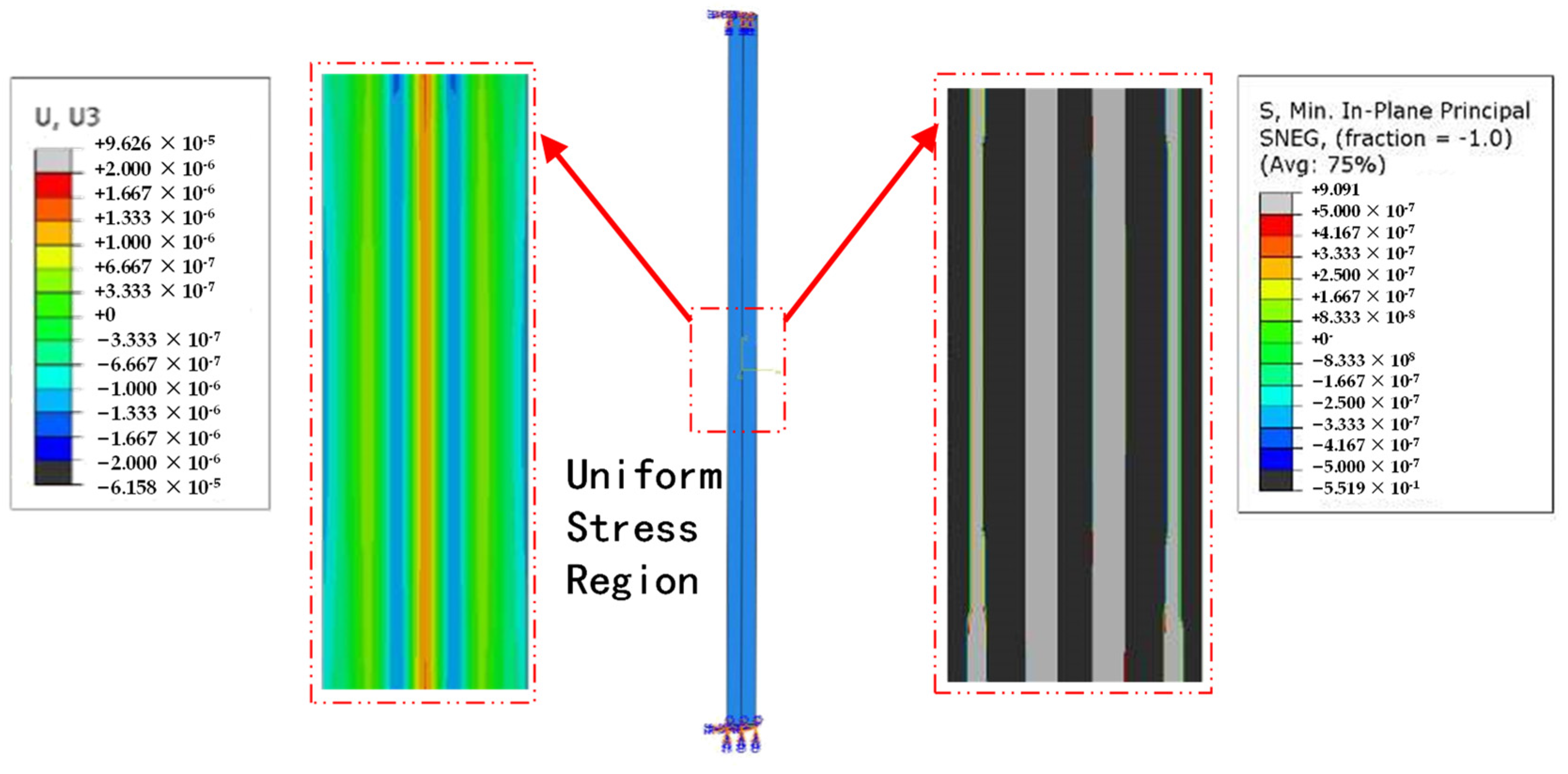
2.1. Wrinkling Mechanism of Step-Stiffness Structure

Several methods are widely used to analyze wrinkling in uniform thin films, including stress analysis, initial imperfection buckling simulations, and energy competition mechanisms. In this section, the wrinkling deformation of stiffness-stepped film structures is analyzed based on the energy competition mechanism [12].

To analyze wrinkling deformation induced by buckling, the film should not be treated as a membrane with zero bending stiffness, but rather as a thin plate considering bending stiffness, the film as a thin-plate (its thickness being much smaller than the other dimensions), and satisfying the Kirchhoff–Love hypotheses and the small-deflection assumption.

The analysis of a single wrinkle stripe is performed using an energy-based formulation, calculating the energy associated with stretching along the wrinkle direction and bending along the wrinkle wavelength direction. Considering wrinkle patterns in Figure 1.

$$U_b={\displaystyle \frac{1}{2}}{\displaystyle \underset{\mathsf{\Omega }}{\int }D\left[{\left(\frac{{\partial }^{2}w}{\partial x^2}\right)}^2+{\left(\frac{{\partial }^{2}w}{\partial y^2}\right)}^2+2\upsilon \frac{{\partial }^{2}w}{\partial x^2}\frac{{\partial }^{2}w}{\partial y^2}\right]}d\mathsf{\Omega }$$

(1)

In the equation, $U_b$ denotes the bending energy of the film, w denotes the out-of-plane deformation (which can often be expressed as a polynomial or trigonometric function; for the wrinkle problem, w is also a function of the wrinkle wavelength λ and amplitude A, and the function mode of w could be $w\left(x,y,\lambda ,A\right)$), D denotes the stiffness matrix $D={\displaystyle \frac{E{t}^3}{12\left(1-{\nu }^2\right)}}$, $l,\lambda$ represent the length and width of the wrinkle strip, υ is Poisson’s ratio, E is Young’s modulus, and t is the structure thickness.

$$U_s={\displaystyle \underset{\mathsf{\Omega }}{\int }{\sigma }_x{\epsilon }_x+{\sigma }_y{\epsilon }_y}d\mathsf{\Omega }={\displaystyle \frac{1}{2}}{{\displaystyle \underset{\mathsf{\Omega }}{\int }{T}_x\left(\frac{\partial w}{\partial x}\right)}}^2+T_y{\left({\displaystyle \frac{\partial w}{\partial y}}\right)}^{2}d\mathsf{\Omega }$$

(2)

In the equation, $U_s$ represents the bending energy of the film, $T_x$ is the tensile force in the x-direction, and $T_y$ is the tensile force in the y-direction.

Based on Equations (1) and (2), one obtains

$$\mathsf{\Pi }=U_s+U_b$$

(3)

In the equation, $\mathsf{\Pi }$ denotes the total potential energy of the film.

Based on the energy method, to solve for the unknowns in the above expression, one takes its partial derivatives and sets them equal to zero. For example, let ${\displaystyle \frac{\partial \prod }{\partial \lambda }}=0$.

Because the tensile load in an infinitely long film structure is uniformly distributed, it can be assumed that there is no bending strain along the long-edge direction, then the out-of-plane deformation trial function can be assumed as follows:

$$w\left(x,y,A,\lambda \right)=A\sin \left({\displaystyle \frac{2\pi y}{\lambda }}\right)$$

(4)

Assume an infinitely long film structure whose wrinkling can be considered as strips of wavelength λ uniformly distributed along the short-edge direction. The corresponding energy can then be calculated using the following formula:

$$U_b={\displaystyle \frac{1}{2}}{\displaystyle \underset{\mathsf{\Omega }}{\int }D{\left(\frac{{\partial }^{2}w}{\partial y^2}\right)}^2}d\mathsf{\Omega }={\displaystyle \underset{0}{\overset{L}{\int }}{\displaystyle \underset{0}{\overset{W}{\int }}\frac{1}{2}}}D{\left({\displaystyle \frac{{\partial }^{2}w}{\partial y^2}}\right)}^{2}dxdy$$

(5)

$$U_s={\displaystyle \frac{1}{2}}{{\displaystyle \underset{\mathsf{\Omega }}{\int }{T}_y\left(\frac{\partial w}{\partial y}\right)}}^{2}d\mathsf{\Omega }$$

(6)

Therefore, the total potential energy can be expressed as

$$\prod ={\displaystyle \underset{0}{\overset{L}{\int }}{\displaystyle \underset{0}{\overset{W}{\int }}\left[\frac{1}{2}D{\left(\frac{{\partial }^{2}w}{\partial y^2}\right)}^2+T_y{\left(\frac{\partial w}{\partial y}\right)}^2\right]}}dydx$$

(7)

In this expression, A denotes the wrinkle amplitude, and λ denotes the wavelength, which can also be written as $\lambda ={\displaystyle \frac{W}{n}}$.

By substituting (7) into (6), one obtains

$$\prod ={\displaystyle \frac{1}{2}}LW{A}^2\left[D{\left({\displaystyle \frac{2\pi }{\lambda }}\right)}^4+T_y{\left({\displaystyle \frac{2\pi }{\lambda }}\right)}^2\right]$$

(8)

To determine the wavelength λ, the equation is

$${\displaystyle \frac{\partial \mathsf{\Pi }}{\partial \lambda }}=LW{A}^2\left[-2D{\left({\displaystyle \frac{2\pi }{\lambda }}\right)}^5-T_y{\left({\displaystyle \frac{2\pi }{\lambda }}\right)}^3\right]$$

(9)

Moreover, the force in the y-direction is generated by the Poisson effect, yielding $T_y<0$, which could be expressed as $T_y=-\upsilon T_x=-\upsilon F$. If the force in the x-direction is F and Poisson’s ratio of the infinitely long film structure is υ, then

$${\displaystyle \frac{\partial \mathsf{\Pi }}{\partial \lambda }}=LW{A}^2\left[-2D{\left({\displaystyle \frac{2\pi }{\lambda }}\right)}^5+\upsilon F{\left({\displaystyle \frac{2\pi }{\lambda }}\right)}^3\right]$$

(10)

By setting Equation (10) equal to 0, the wavelength is obtained as

$$\lambda =2\pi \sqrt{{\displaystyle \frac{2D}{\upsilon F}}}$$

(11)

The wavenumber can be determined from the ratio of the film structure’s width to the wavelength.

To validate the analytical results, finite element simulations were conducted. In ABAQUS 2020, a film with a large aspect ratio of 1000:40 was modeled (the length was set to 1000 mm and the width was set to 40 mm), the mesh length was set at 1 mm, element type was set as S4R. Buckle analysis was analyzed firstly, and the keywords “*imperfection” were used to set the buckle mode to analyze the wrinkle results. The central region of the film was used to analyze the uniform wrinkle patterns. As shown in Figure 2, three full wrinkle wavelengths appear at the center of the sheets. Figure 2 (left) presents the out-of-plane displacement U, U3 of the tensioned membrane under axial loading, highlighting the wrinkle amplitude across the central region. Figure 2 (right) shows the distribution of the minimum in-plane principal stress (SNEG), which captures the compressive stress concentrations induced by wrinkling. Using the material parameters—a film thickness of 50 µm and Young’s modulus of 3 Gpa—as well as the loading boundary, a tensile load of 58 N, Equation (11) predicts a wavelength of 11.89 mm. Since the specimen width is 40 mm, only three complete wrinkle wavelengths can be accommodated across the membrane. This geometric constraint directly fixes the number of wrinkles at n = 3. This result matches the simulation results and confirms the validity of the approach (10.96 mm in ABAQUS results). For an infinitely long film, the amplitude A can only be determined by substituting the deflection profile into the energy expression to find its extremum, since in Equation (8), any choice of A does not affect the derivative’s root.

Because the tensile load on the thin-film stirp is relatively small, the bending moment induced by the copper foil and the tensile load’s effect on the film deformation can be treated independently. So, the step-stiffness structure can be regarded as a pure thin-film under tensile and bending load (ignoring the surface interfacing problem, since the loading leads to a small strain distribution). In other words, the boundary condition of the film can be represented as a superposition of (1) the bending deformation imposed by the copper foil and (2) the original tensile load acting on the film. Summing these two effects yields the wrinkle analysis model for the stiffness-stepped film structure.

The generation of the bending moment can then be derived from the copper foil’s structural parameters, and the expression is as follows:

$$U_{bc}={\displaystyle \frac{1}{2}}{\displaystyle \underset{\mathsf{\Omega }}{\int }{M}_x{\kappa }_x+M_y{\kappa }_y+M_{xy}{\kappa }_{xy}}d\mathsf{\Omega }$$

(12)

In the equation, $U_{bc}$ represents the bending strain energy introduced by the copper foil, and $M_i,{\kappa }_i\left(i=x,y,xy\right)$ denote the bending moments and curvatures in the respective directions. The curvature can be obtained from the thin-plate deflection formula in elasticity theory, i.e., by taking the second derivative of the assumed deflection function.

In summary, the energy-based wrinkling analysis model for the stiffness-stepped film structure can be expressed as follows:

$$\prod =U_s\left({\epsilon }_x,{\epsilon }_y,A,\lambda \right)+U_b\left({\epsilon }_x,{\epsilon }_y,A,\lambda \right)+U_{bc}\left(F,t,w_c\left(x,y\right)\right)$$

(13)

In the above equation, $w_c\left(x,y\right)$ denotes the out-of-plane deflection distribution function arising from bending, which does not contain the influence of wrinkling (λ and A). For the stiffness-stepped film, the copper foil is only effectively subjected to bending moments (under small loading), while the four edges carry asymmetric in-plane loads, so the bending moment magnitudes at each edge differ. This spatial variation in moment makes it challenging to obtain the numerical solution of the model. For such complex cases, the finite element method is recommended for analysis.

For an infinitely long film, assuming that the bending moment $M_x$ induces curvature deformations ${\kappa }_{xb}$, ${\kappa }_{yb}$, the new strain energy can be expressed as

$$\prod ={\displaystyle \frac{1}{2}}LW{A}^2\left[D{\left({\left({\displaystyle \frac{2\pi }{\lambda }}\right)}^2+{\displaystyle \frac{{\kappa }_{yb}^2}{A^2}}\right)}^2+T{\left({\displaystyle \frac{2\pi }{\lambda }}\right)}^2\right]+{\displaystyle \frac{1}{2}}DLW{\kappa }_{xb}^2$$

(14)

By taking the partial derivatives, one obtains

$${\displaystyle \frac{\partial \mathsf{\Pi }}{\partial \lambda }}=LW{A}^2\left[-2D{\left({\displaystyle \frac{2\pi }{\lambda }}\right)}^5-4D{\displaystyle \frac{{\kappa }_{yb}^2}{A^2}}{\left({\displaystyle \frac{2\pi }{\lambda }}\right)}^3+\upsilon F{\left({\displaystyle \frac{2\pi }{\lambda }}\right)}^3\right]$$

(15)

By setting Equation (15) equal to zero, the wrinkle parameter for the wrinkled region of an infinitely long film under the influence of a bending moment is given by

$$\lambda =2\pi \sqrt{{\displaystyle \frac{2D}{\upsilon F-4D\frac{{\kappa }_{yb}^2}{A^2}}}}$$

(16)

In the above expression, ${\kappa }_{yb}$ denotes the curvature in the y-direction obtained from the independent bending–coupled strain calculation. The amplitude A is determined by substituting the deflection function w into the potential-energy expression for an infinitely long film without bending moments and finding its extremum. Analysis of Equation (16) shows that as the denominator decreases, the wavelength λ increases; when the denominator reaches zero, wrinkle deformation disappears, and the structural response degenerates to a pure bending, biaxially coupled deformation mode without wrinkling. Assuming an infinitely long film is subjected to a uniform 1° rotation deformation about the x-axis, the resulting wrinkle wavelength can be calculated as 14.3 mm. The finite element simulation results yielded an approximate wavelength of 15.9 mm, demonstrating the validity of the FEM method. The subsequent analysis was carried out using the finite element method verified in this section because the analytical solution is difficult to obtain due to the complexity of the boundary conditions.

The approximately 8% deviation in wrinkle amplitude is primarily caused by the numerical initial imperfection imposed via the buckling eigenmode: this seeding mechanism generates a non-uniform wrinkle pattern that amplifies boundary wrinkle growth and biases the predicted amplitudes. A secondary contribution stems from localized stress concentrations around the clamping fixtures, which induce additional non-uniform wrinkles that propagate inward and further perturb the membrane’s central region.

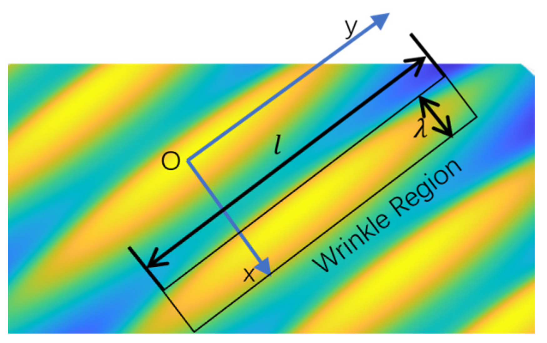
2.2. Surface Deformation of STMA

The typical shape of a Space Tensioned-Membrane Antenna (STMA) includes two layers: phased array patches are set on the up layer, and a ground patch is set on the down layer. The stiffness step structure easily causes out-of-plane deformation, such as wrinkling deformation and bending deformation. Both the deformations lead to changes in the spacing of the two layers. The spacing of two layers is a design parameter required for electromagnetic performance, so determining the extent to which deformation influences electromagnetic performance is essential for tensioned-membrane antenna.

Figure 3 shows the possible deformation types of the up layer. As the membrane antenna is stretched at corners, the stress concentration easily leads to wrinkling deformation. Futhermore, fabrication errors also cause changes. To determine reliable results of out-of-plane deformation of STMA, a simulation and experiment were carried out.

Because the effectiveness of the finite-element approach was confirmed in the previous section, we employed finite-element analysis to compute the surface deformation of the more complex structure. The model was built in ABAQUS 2020.

To ensure numerical accuracy, the 7 × 3 suspension-cable configuration (m × n cables represent the number of complete catenaries in the horizontal and vertical directions) uses the following mesh counts: the array-layer film has 105,974 elements, and the radiator layer has 100,252 elements; the supporting frame has 66,474 elements; each support beam has 6534 elements × 2 beams; and each connection flange has 4629 elements × 4 flanges.

The 5 × 3 suspension-cable configuration uses 104,211 elements for the array-layer film and 99,886 elements for the radiator layer; its supporting frame again has 66,474 elements, each support beam is 6534 × 2, and each flange is 4629 × 4. The tension cables are modeled with connector elements, and the copper foil antenna on the film is implemented via a composite lamination.

All elements’ length settings were verified by increasing the number of elements until the simulation results converged. All membrane regions used the S4R element, and the support beam, frame, and connection flange used the S3 element. The material properties are shown in

Table 1. Antenna’s material parameters.

Part	Material Parameters
	Material	Young’s Modulus	Poisson Ratio
Membrane	Polymide	3 GPa	0.33
Beam/Frame/Connection flange	Alumimum	206 GPa	0.3
Truss	Carbon Fiber	110 GPa	0.32

.

The loading method of the structure uses the cooling method on the tension cable, that is, giving a thermal expansion coefficient and calculating the temperature change range corresponding to a given tension force. This method can be used to apply tension to the rope finite element structure. We applied a post-buckling finite-element analysis based on the initial buckling-mode defect method. First, a stress analysis was performed; next, the buckling modes were computed; finally, the primary buckling mode was introduced into the model as an initial imperfection via keyword modification in ABAQUS. This procedure yields the wrinkling pattern analysis of the thin-film structure.

Based on existing references, it can be determined that different thicknesses of the membrane were set to analyze material parameters’ influence on out-of-plane deformation. Both the thickness and patch size are essential factors for out-of-plane deformation types [27].

Figure 4 shows the out-of-plane displacement contours for the 7 × 3 suspension-cable configuration. On the left is the array-layer film contour: as the prestress increases, the zones of maximum deformation expand from the four corner tension points to all tension points. The deformation in the copper foil-plated area of the array antenna becomes progressively more pronounced, with its peak value rising from 0.05 mm to 0.19 mm. Near the boundaries, the copper foil region exhibits even larger displacements, a consequence of the composite structure’s edge constraints. The deformation pattern of the copper foil patch clearly reflects the growing tension–bending coupling effect under higher tensile loads.

On the right of Figure 4 is the radiator-layer film contour: with increasing prestress, the region of maximum deformation consistently occurs at the inner suspension cables, and its extreme value increases from 0.36 mm to 0.66 mm. Deformation in the copper-clad region also becomes more evident, with its peak rising from 0.38 mm to 0.70 mm. The maximum and minimum value information is summarized in

Table 2. Maximum deformation vs. prestress.

Prestress/N	Maximum Deformation/mm
	5 × 3 Suspension Cable Configuration		7 × 3 Suspension Cable Configuration
	Radiator Layer	Ground Layer	Radiator Layer	Ground Layer
1.0	0.6332	−0.4000	0.3698	−0.3807
2.1	1.117	−0.8091	0.6395	−0.6479

.

Figure 5 presents the out-of-plane displacement contours for the 5 × 3 configuration. The left panel (array layer) exhibits a deformation pattern similar to that of the 7 × 3 case but with larger magnitudes: the copper foil region’s peak displacement increases from 0.10 mm to 0.30 mm. The right panel (radiator layer) shows that the maximum deformation remains centered on the internal suspension cables, growing from 0.63 mm to 1.10 mm as prestress rises, while the copper foil region’s peak displacement increases from 0.40 mm to 0.88 mm.

Combining the thin-film antenna deformation characteristics shown in Figure 4 and Figure 5, it can be seen that the upper antenna exhibits more pronounced local deformations with the periodic features of the repeating array units. In contrast, the patch area of the lower antenna shows small-amplitude, uniformly distributed deformations. Therefore, to analyze how structural deformation affects the antenna’s electrical performance, one can focus on a representative unit—namely, a single patch element of the antenna. Furthermore, given the deformation magnitude of the upper film, the out-of-plane deformation of the lower film may be neglected for a simplified analysis.

2.3. Dual-Domain Displacement-Driven Function

The out-of-plane deformation characteristics of the upper film and out-of-plane deformation characteristics of the upper film, and the deformation behavior of the step-stiffness thin-film structure is jointly influenced by both the film’s and the patch’s stiffness [27]. Thus, deformation is composed of two parts—one is the patch area and the other is the membrane area. The deformation of the patch area mainly shows bending deformation. The deformation of the membrane area is of the Fourier type. So, extracting ABAQUS simulation result data (as shown in Figure 4 and Figure 5) with a typical patch area (as shown in Figure 6), MATLAB 2019b can be used for complex function construction and fitting in a two-region domain.

This treatment is consistent with existing research findings, namely, that the material stiffness of the film and patch regions influences the structure’s deformation morphology.

$$f\left(x,y\right)=cfz1{\displaystyle \sum _{i,j}^n{x}^i{y}^j}+cfz2{\displaystyle \sum _{k,l}^n\cos (kx)\mathrm{s}\mathrm{i}\mathrm{n}(kx)+\cos (ly)\mathrm{s}\mathrm{i}\mathrm{n}(ly)}$$

(17)

Different material parameters lead to different forms of out-of-plane deformation of stiffness step films, but the overall picture can be abstracted into two variables—film and patch stiffness. Therefore, in this study, a two-domain displacement model is adopted to approximate characterize the deformation of the stiffness-step thin-film shaped surface.

The antenna unit deformation patterns corresponding to the 20th-order fitting results are given in Figure 7 The center patch region deformation and the outer film region wrinkle deformation were independently controlled using two parameters. Using this function, antenna deformation could be approximate estimated. In the following sections, electromechanical coupling modeling of the antenna is performed based on this function to analyze the electrical properties of unit and phased array antennas.

3. Structural–Electromagnetic Coupling Model

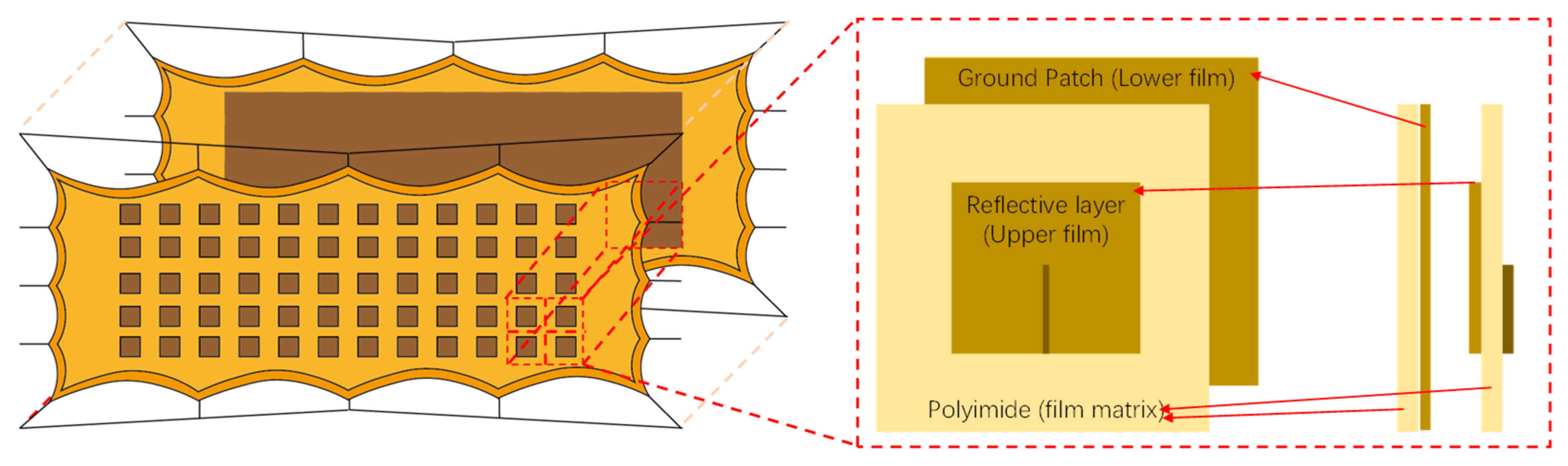
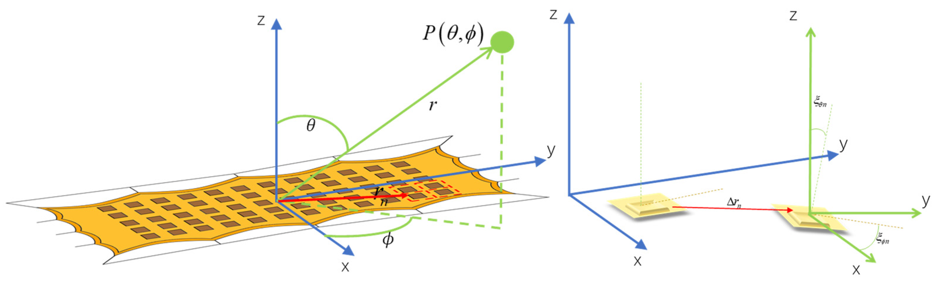
3.1. Electromechanical Coupling Model

The coordinate system used for analyzing the far-field electrical performance of the phased array antenna is given in Figure 8. According to the theory of antenna design and analysis, the formula for calculating the field strength at point P is shown in the following equation [18].

$$E\left(r,\theta ,\varphi \right)={\displaystyle \frac{-j\omega {\mu }_0}{4\pi r}}{\displaystyle \underset{dS}{\int }{J^{\prime }}_n\left(x,y\right)e^{-jkr\cdot }\cos \theta dS}$$

(18)

In the equation, $J_n(n=1,2,\dots ,\mathrm{N})$ denotes the current density of the nth patch, ω is the angular frequency, ${\mu }_0$ is the vacuum permeability, $\theta ,\varphi$ is the observation direction at point P in space, k is the propagation constant (wavenumber), and $\stackrel{⌢}{r}={\displaystyle \frac{\mathrm{r}}{r}}=$ $(\sin \theta \cos \varphi ,\sin \theta$$\sin \varphi ,\cos \theta )$ is the unit vector in the radial (r) direction.

According to the antenna design theory, the change in patch area displacement affects the spacing between the radiating patch and ground plane of the thin-film antenna, thus affecting the electrical performance of the antenna. And the effect of fold deformation in the film region represents the deformation in the medium region. In the equation, this deformation has an effect on antenna performance, but the effect of this deformation on the electrical performance has not been analyzed in previous studies.

The formula for calculating the nth patch antenna’s electrical performance, accounting for deformation, is as follows:

$$E\left(r,\theta ,\varphi \right)={\displaystyle \frac{-j\omega {\mu }_0}{4\pi \left(r+\Delta r\right)}}{\displaystyle \underset{dS}{\int }{J}_n\left(x,y\right)e^{-jkr\cdot }{e}^{j\Delta \phi \left(x,y\right)}\cos \theta dS}$$

(19)

In the formula, $\Delta r$ and $\Delta \phi$, respectively, denote the effects introduced by the structural deformation. Here, $\Delta r$ and $\Delta \phi$ represent the deformation errors in displacement and rotation, respectively. $\Delta r$ and $\Delta \phi$ are, respectively, extracted from the overall antenna displacement function. $\Delta r$ and $\Delta \phi$ can be expressed as

$$\begin{array}{l}\left\{\begin{array}{c}\Delta r={\displaystyle \frac{1}{S_{\mathrm{patch}}}}{\displaystyle \underset{S_{\mathrm{patch}}}{\iint }{f}_{patch}\left(x,y\right)dS}\begin{array}{cc}& \end{array}{f}_{patch}\left(x,y\right)=c_{fz1}{\displaystyle \sum _i{x}^i{y}^i}\\ \Delta \phi \left(x,y\right)=\arccos \left[\widehat{n}\left(x,y\right)\cdot {\widehat{r}}_0\right]=\arccos \left({\displaystyle \frac{1}{\sqrt{1+{\left({\partial }_{x}f\right)}^2+{\left({\partial }_{y}f\right)}^2}}}\right)\approx {\displaystyle \frac{{\left({\partial }_{x}f\right)}^2+{\left({\partial }_{y}f\right)}^2}{2}}\end{array}\right.\\ \end{array}$$

(20)

Equation (20) follows directly from the small-slope geometry sketched in Figure 8. Denoting the local surface profile by f(x,y), the height change of each patch, Δr, is obtained by averaging the patch deflection over the patch area $S_{patch}$. The phase shift $\Delta \phi$ is then the angle between the deformed normal ${\widehat{n}}_i$ and the reference normal ${\widehat{n}}_0$, where the final approximation is valid for $\partial f\ll 1$.

When the electrical performance of a single patch unit is obtained, the electrical performance of the entire antenna can be obtained through Equation (21).

$$E_{Ant}={\displaystyle \underset{n,m}{\iint }E\left(n,m\right)e^{j(k_x{x}_{mn}+k_y{y}_{mn})}}$$

(21)

In this equation, n and m represents the number of rows and columns. The sum represents the vector sum.

In this paper, the effects of two typical deformations on the electrical properties of the patch antenna unit are investigated separately by varying the parameters of the two dual-domain displacement patterns.

Since the film scale of thin-film antennas is particularly small compared to the area, direct modeling in simulation software results in a huge amount of computation. In this paper, we adopt the mode of importing the results of unit calculation by Ansys HFSS into MATLAB for superposition calculation to predict the performance of a phased array antenna. In Equation (21), E(n,m) is the complex far-field contribution of the (n,m) patch and is indeed obtained from Equation (19). In our workflow, a full-wave HFSS simulation is first performed on a single deformed patch to evaluate E(n,m) in Equation (19). From this, the complex amplitude E(n,m) (magnitude and phase) is extracted. These per-element values are then exported to MATLAB, where Equation (21) is implemented to compute the array sum $E_{Ant}$ and thus predict the phased array pattern under the given deformation. This two-step procedure ensures that the element-level HFSS results feed directly into the array-level MATLAB post-processing.

All HFSS simulations use a single representative patch to enable rapid, order-of-magnitude estimates of gain and impedance errors; inter-element coupling is omitted because full-array simulations would incur excessive computational cost and significantly longer run times.

3.2. Patch Electro-Magnetic Performance Simulation

The simulation analysis first focuses on a single antenna unit; the array antenna analysis is then conducted by exporting the data and performing superposition calculations in MATLAB based on formula (21) and patch results from HFSS. For a patch size of 98 mm × 98 mm and a film spacing of 12.7 mm, analysis of a representative patch unit yields the antenna’s reflection coefficient and its E and H plane gain patterns. Simulation was carried out using Ansys HFSS. A patch length of 98 mm was selected, corresponding to approximately 0.425λ at the center frequency of 1.3 GHz. This dimension provides a practical trade-off between structural rigidity, radiation efficiency, and integration requirements within our deployable membrane antenna platform. It is also consistent with the patch configurations used in related institutional engineering projects.

It is worth noting that several simplifications were adopted in the current electromagnetic simulation framework. First, mutual coupling effects between adjacent antenna elements were not considered in the array-level analysis. The radiation pattern was obtained through the superposition of isolated element responses, assuming negligible interaction. This approach is commonly used in preliminary parametric studies, but may overestimate the array performance in practical scenarios with strong inter-element coupling.

Second, the structural deformation used in the electromechanical coupling model was derived under static assumptions. The influence of dynamic factors such as deployment vibrations, thermal-induced fluctuations, or time-varying disturbances was not incorporated. While the static assumption provides a tractable means of evaluating the deformation-induced gain degradation, it may not fully capture transient behavior encountered in orbit.

Third, the material properties of the membrane and conductive layers were treated as ideal and invariant during simulation. Effects due to temperature variations, radiation aging, or material nonlinearity were not included. These assumptions simplify the model and reduce computational cost but may introduce discrepancies in long-term or extreme-environment conditions.

Despite these simplifications, the current framework provides valuable insight into the sensitivity of antenna gain and beam steering to structural deformations. Future work will consider mutual coupling effects, dynamic structural responses, and realistic material behavior to enhance the fidelity of the model.

The antenna model was constructed in HFSS with standard microstrip patch geometry using sheets and PEC (Perfect Electric Conductor) material for the patch and ground, along with a dielectric substrate modeled using the membrane with solids with polymide parameters. Radiation boundaries were applied to enclose the entire simulation domain, with a minimum distance of λ/4 from the structure. A lumped port was used for excitation. The frequency sweep was set from 1.2 GHz to 1.6 GHz using a discrete sweep with a 10 MHz step.

Regarding meshing, the default adaptive meshing strategy in HFSS was used. This includes a convergence criterion of ΔS = 0.02 and a minimum of 2 and a maximum of 15 adaptive passes. Since the deformation was quite small compared with the patch length, no manual mesh operations were applied, and the software automatically refined the mesh near edges and the feed region. These settings were sufficient to ensure accurate convergence and are consistent with the best practices for planar antenna modeling.

The simulation results are shown in Figure 9. It can be seen that the reflection coefficient S11 achieves a good matching depth at 1.3 GHz, with approximately −12 dB. In both the E-plane and H-plane, the antenna attains a gain level of approximately 7.5 dB.

Next, a hypothetical independent deformation analysis of the film and patch regions was performed, first identifying the extent to which each region impacts the electrical performance of the patch.

As shown in the S-parameter (S11) curves in Figure 10, when $d_{pch}$ = 0 mm, the antenna achieves its best match around 1.28 GHz, with the minimum S11 reaching approximately −12 dB, indicating optimal resonance and impedance matching. As $d_{pch}$ is reduced in 0.2 mm steps from 0 to −1 mm, the resonant frequency first shifts downward to 1.24 GHz, then returns to the 1.28–1.30 GHz range. Over this range, the S₁₁ minimum oscillates between −9 dB and −16 dB, showing that matching gradually degrades as the patch is translated downward. Moreover, at $d_{pch}$ = −0.4 mm, a small additional dip appears near 1.6 GHz, suggesting the excitation of a parasitic mode and potential multi-band behavior that could interfere with single-band operation in the 1.24–1.30 GHz band.

In the gain radiation patterns shown in Figure 10, $d_{pch}$ = 0 mm yields the highest main lobe gain of about 6.5 dB, with low sidelobe levels and a symmetric pattern. As $d_{pch}$ decreases from −0.2 mm to −1 mm, the main lobe gain drops noticeably, falling to around 5 dB at $d_{pch}$= −1 mm and shifting off-axis from θ = 0°. At the same time, the sidelobe levels around θ ≈ ±150° rise by about 0.2 dB, and the pattern’s symmetry degrades. This indicates that shifting the patch alters the current distribution and thereby distorts the far-field radiation pattern, affecting both the main and sidelobes. In a phased array application, such unit-level misalignments can degrade overall beam-scanning accuracy and increase sidelobe interference.

Based on the phase change analysis theory [28], the phenomenon of the gain main lobe splitting into two in Figure 10 can be explained by the following process.

When each patch is laterally translated by $d_{pch}$, its radiated field acquires an extra path-length phase shift $\Delta \varphi \left(\theta \right)=k{d}_{pch}\cos \theta$. For $d_{pch}$ = 0, the aperture phase front remains planar, yielding a single boresight beam. As soon as $d_{pch}$ ≠ 0, this uniform phase ramp tilts each element’s pattern off broadside. If the phase gradient places a null at θ = 0, the main beam splits into two symmetric lobes. Since every element undergoes the same translation, the array reproduces two lobes around broadside for all non-zero $d_{pch}$.

According to the equivalent-circuit model [29], a slight variation (±1 mm) in the probe-to-ground-plane spacing significantly alters the probe’s series inductance, causing shifts of tens of ohms in both the real and imaginary parts of the input impedance. This leads to a sudden rise in VSWR and severe mismatch, ultimately distorting the patch current distribution and producing beam splitting with a dual-peak radiation pattern. Furthermore, Mohammed et al. [30] emphasize that minute perturbations in feed-geometry parameters such as probe length and substrate thickness can excite parasitic modes or feedline radiation, thereby elevating sidelobe levels and flattening the main beam.

In summary, as the patch position shifts from 0 mm to −1 mm, not only does the resonant frequency oscillate and matching degrade, but the main lobe gain also falls, and the radiation pattern deteriorates. Therefore, in phased array antenna design and fabrication, patch-position deviations must be tightly controlled to ensure uniform matching and gain across all elements, thereby achieving optimal beam patterns and array performance.

As shown in the S-parameter (S11) curves in Figure 11, as $d_{zm}$ increases, the antenna’s matching characteristics change noticeably. At $d_{zm}$ = 0 mm (no translation), the resonant frequency is near 1.28 GHz with S11 ≈ −12 dB, indicating good matching. However, when $d_{zm}$ increases to −5 mm, the resonant frequency shifts toward 1.30 GHz, and S₁₁ becomes smaller. This behavior shows that the film’s vertical position alters the antenna’s effective dielectric constant and electric-field distribution, thereby changing the resonance and matching.

As shown in the gain radiation patterns in Figure 11, at $d_{zm}$ = 0 mm, the main lobe gain is highest and sidelobe levels are relatively low, indicating optimal radiation performance. As $d_{zm}$ increases, the pattern symmetry degrades, exhibiting a double peak near the main lobe, while sidelobe levels remain largely unchanged. This reduces the beamforming resolution.

In summary, translation of the film ($d_{zm}$) significantly affects the antenna’s resonant frequency and matching and influences the symmetry and sidelobe characteristics of the gain pattern. In phased array applications, large variations in $d_{zm}$ between elements can lead to pattern distortion and increased beam scan errors. Therefore, during design and fabrication, film positioning must be tightly controlled to ensure consistent element matching and beamforming accuracy, preventing performance degradation due to film displacement.

4. Discussion

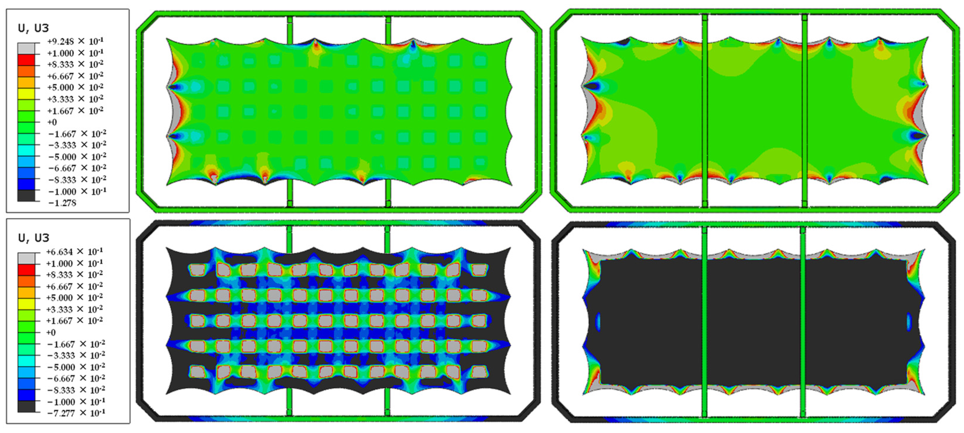
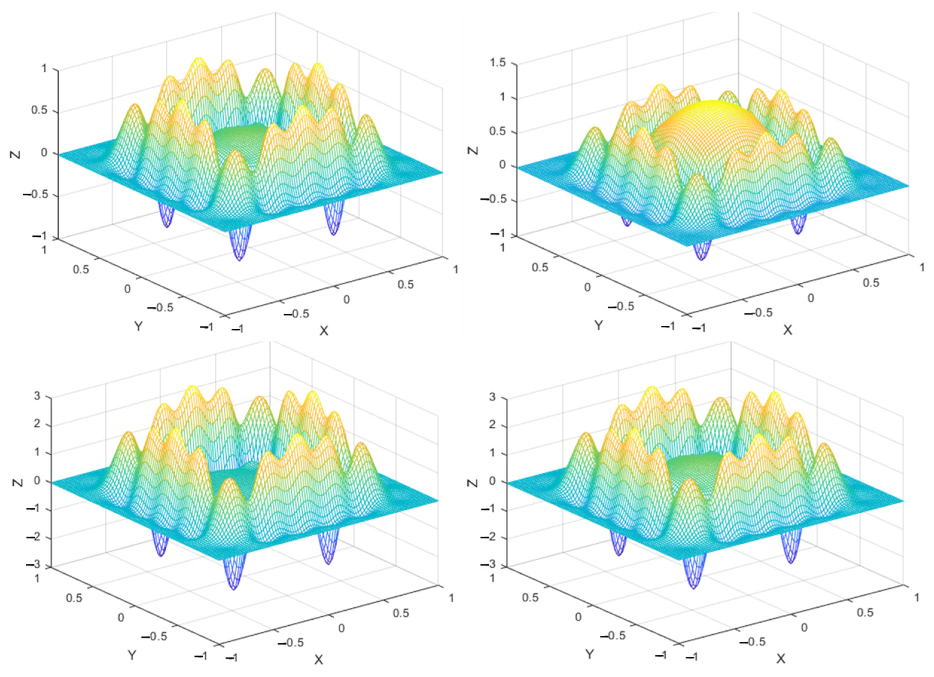
4.1. Dual-Domain Displacement Patch Analysis

Firstly, we performed the analysis of Equation (17) under the condition $c_{fz1}$ = $c_{fz2}$, thereby predicting the effect of local deformation of the patch antenna on its electrical performance.

The impact of local film deformation ($c_{fz1}$) on antenna performance was analyzed separately via S-parameter (S11) curves and gain radiation patterns. As shown in Figure 12, the S11 curves depict how the antenna’s reflection coefficient varies with frequency for different $c_{fz1}$ values. Figure 12 shows the antenna gain versus θ at 1.4 GHz under the same $c_{fz1}$ conditions.

In Figure 12, changing $c_{fz1}$ causes clear shifts in both the resonant frequency and matching depth: for certain $c_{fz1}$ values, the resonance moves to higher frequencies, and the S11 minimum degrades from about −12 dB to −6.7 dB. This indicates that local deformation alters the patch’s effective electrical length and impedance environment, worsening matching or shifting the resonance. At $c_{fz1}$ = 0.003, no S11 response appears between 1 GHz and 2 GHz, implying the resonance has moved outside this band or become unmatched.

The gain patterns in Figure 12 illustrate the far-field behavior at 1.4 GHz for each $c_{fz1}$. The blue curve ($c_{fz1}$ = 0.003) shows an unreasonably low main lobe gain and uneven sidelobe distribution, indicating that this deformation severely distorts the current distribution and polarization, effectively degrading radiation performance. Other cases (e.g., the green and orange curves) maintain smoother patterns, though with a reduced peak gain.

The phenomenon that the gain decreases first and then increases can be qualitatively analyzed using the following equations.

When the surface distortion increases to $c_{fz1}$ = 0.003, due to the geometric changes in the patch-ground gap and the current path, the equivalent capacitance and inductance of the antenna increase simultaneously, causing the resonant frequency to shift out of the original design frequency band in the low-frequency direction; at the same time, the distortion enhances the excitation of high-order modes and the patch–film coupling, significantly reducing the quality factor, making the original S₁₁ matching valley shallow and wide, and making it difficult to distinguish within a given scanning range. This mechanism can qualitatively explain why no obvious matching point can be seen at 0.003.

Based on the previous section’s analysis, among the three offset errors, the $c_{fz1}$ error has the most significant impact on resonant frequency drift. As the $c_{fz1}$ offset increases, the resonant point shifts the furthest and may even fall outside the matching band, preventing the antenna from operating normally at its design frequency and undermining system stability. It also inflicts the greatest direct damage to gain—distorting the pattern and even exceeding the ideal peak—indicating that the form of local deformation represented by $c_{fz1}$ is the most severe. In high-precision applications (e.g., satellite communications or phased arrays), such frequency drift can cause element-to-element phase mismatches, thereby degrading overall directivity and gain balance.

In general, local deformation of the film leads to shifts in the resonant frequency and matching characteristics and causes varying degrees of distortion or sidelobe increase in the gain pattern. For a phased array antenna, if such deformation varies significantly between elements, it can degrade beam-forming precision and compromise pattern consistency. Therefore, during design and fabrication, the film’s local deformation must be strictly controlled to ensure each element’s matching and gain remain stable.

In contrast, the $d_{pch}$ error ranks second in severity. It not only shifts the resonant frequency but also significantly worsens matching and reduces far-field gain, leading to lower antenna efficiency and making it a primary contributor to electrical performance degradation. The $d_{zm}$ error has the mildest effect; as seen in the gain patterns and S11 curves, its main impact appears to be on the system’s radiation uniformity, with little effect on resonance or matching.

In summary, the $c_{fz1}$ error has the most direct impact on resonant frequency and should be prioritized to avoid system-level instability caused by frequency drift; the $d_{pch}$ error significantly affects matching and gain, requiring strict control of manufacturing precision; the $d_{zm}$ error poses relatively mild harm but still warrants attention for its effect on far-field radiation. During antenna design and fabrication, the impacts of these errors should be comprehensively considered to ensure system stability and reliable performance.

4.2. Phased Array Antenna Analysis

We now vary the values of $c_{fz1}$ and $c_{fz2}$ to predict the electrical performance of the phased array antenna; when $c_{fz1}$ = 0.001 and $c_{fz2}$ = 0.0012, the resulting structural deformation of the array layer most closely matches that shown in Figure 4.

The unit performance variations are shown in Figure 13. When studying the effects of the structural parameters $c_{fz1}$ and $c_{fz2}$ on the unit antenna gain, gain-versus-angle curves were plotted for the E-plane (ϕ = 0°) and H-plane (ϕ = 90°) for different $c_{fz1}$–$c_{fz2}$ combinations. The analysis indicates that variations in $c_{fz1}$ mainly affect the main lobe level of the radiation pattern; variations in $c_{fz2}$ primarily influence the pattern shape and sidelobe levels, with only a minor effect on main lobe gain.

In Figure 13′s four non-normalized unit gain plots, the first and third correspond to the E-plane, while the second and fourth correspond to the H-plane. Overall, when $c_{fz1}$ or $c_{fz2}$ increases, the main lobe gain typically fluctuates between 5 and 8 dB, but the sidelobe and null depths exhibit significant variation with parameter changes.

In the E-plane (Figure 13, first and third plots), the main lobe gain at θ ≈ 0° mostly remains at the 6–7 dB level, although in some cases, the gain decays more sharply ($c_{fz1}$ = 0.001, 0.002), and the sidelobes are mainly concentrated near θ ≈ ±50° and ±100°. As the parameter increases, some curves exhibit a 2–3 dB gain increase at those sidelobe positions or a shift in null locations, indicating that local film deformation or patch translation leads to an uneven current distribution, which, in turn, affects the E-plane sidelobe characteristics. If significant differences exist between elements, array synthesis may suffer amplitude and phase inconsistencies, raising the overall sidelobe level.

In the H-plane (Figure 13, second and fourth plots), the main lobe gain also lies between 5 and 8 dB, but the curves are more sensitive to changes, and certain parameter combinations (e.g., $c_{fz1}$ = 0.003 or $c_{fz2}$ = 0.002–0.003) cause only minor shifts in the main lobe peak, yet produce higher sidelobes near θ ≈ ±70° or deeper nulls near θ ≈ ±100°. Other combinations ($c_{fz2}$ = 0.002) lead to severe fluctuations, blurring the distinction between main and sidelobes. Compared to the E-plane, the H-plane patterns oscillate more strongly, showing that film deformation and local patch displacement more significantly modulate polarization and current distribution in this plane. In phased array applications, such inconsistencies accumulate as amplitude and phase errors in beamforming, degrading beam pointing and sidelobe performance.

In summary, variations in $c_{fz1}$ and $c_{fz2}$ lead to differing degrees of change in the main lobe, sidelobes, and null depths of the gain patterns in the E- and H-planes. While the main lobe gain remains generally stable, the sidelobe levels and null depths are more sensitive to film deformation, whereas copper foil deformation causes more pronounced attenuation of the main lobe. This implies that large $c_{fz1}$ and $c_{fz2}$ deviations between elements can degrade the phased array’s overall sidelobe-suppression capability and beam scanning accuracy. Therefore, in high-precision antenna design and fabrication, $c_{fz1}$ and $c_{fz2}$ must be strictly controlled or calibrated to ensure consistent element gain characteristics and maintain excellent radiation pattern performance.

The apparent discontinuity at θ = ±90° is a numerical artifact of discrete sampling and mesh-cell stitching at the spherical coordinate poles; it does not represent a physical gap and does not affect the main and side-lobe metrics.

As shown in the S-parameter (S11) curves (Figure 14, first plot), when $c_{fz1}$ varies between 0, 0.001, 0.002, and 0.003, the antenna’s matching in the 1.2–1.4 GHz band undergoes significant drift and change. Initially ($c_{fz1}$ = 0 mm), the resonant frequency is about 1.28 GHz, and the S11 minimum reaches approximately −12 dB; as $c_{fz1}$ increases to 0.003, the resonant point oscillates. Meanwhile, the S₁₁ matching depth also changes markedly, indicating that local film deformation shortens the effective electrical length and degrades matching. Furthermore, at $c_{fz1}$ = 0.003, three resonant points appear, the strongest near 1.6 GHz, suggesting excitation of parasitic modes. At $c_{fz1}$ = 0.002, a possible parasitic mode with about –5 dB depth is also seen, though it has limited impact on the main operating band.

As shown in the S-parameter curves (Figure 14, second plot), as $c_{fz2}$ increases from 0 to 0.003, the antenna’s resonant frequency and matching shift sequentially. According to the color legend, $c_{fz2}$ = 0 (red line) shows a main matching dip of about −12 dB near 1.28 GHz; at $c_{fz2}$ = 0.0012 (orange line), the resonance shifts to ≈1.32 GHz, with a minimum of ≈−11 dB; at $c_{fz2}$ = 0.002 (blue line), the resonance shifts most severely to ≈1.45 GHz, with the lowest point of ≈−9 dB; and at $c_{fz2}$ = 0.003 (green line), the main resonance shifts back to ≈1.28 GHz, with a minimum of ≈−8.5 dB. Secondary dips near 1.63, 1.83, and 1.95 GHz (≈−6 dB, −7 dB, −10 dB) appear at $c_{fz2}$ = 0.0012 and 0.003, indicating that local patch deformation excites new parasitic modes. Overall, increasing $c_{fz2}$ causes resonant-frequency oscillation, secondary dips, and a gradual weakening of matching.

As shown in the gain radiation patterns (Figure 14, third plot), at $c_{fz1}$ = 0, the main lobe gain peaks at 7.9 dB, with low sidelobe levels; when $c_{fz1}$ increases to 0.003, the main lobe gain amplitude changes little, but the angle of maximum gain shifts away from θ = 0°, and sidelobes near θ ≈ ±50° rise by about 2–3 dB, reducing pattern symmetry. This shows that local deformation alters the current distribution, boosting radiation at certain angles while causing sidelobe rise or shallower nulls. If such $c_{fz1}$ variations occur between phased array elements, amplitude and phase inconsistencies in beamforming may result, degrading overall beam pointing accuracy and sidelobe suppression. When $c_{fz1}$ = 0.001 mm and 0.002 mm, the gain curve shows significant attenuation at θ = 0°, with the peak gain still near θ = 0°, leading to poorer directivity.

In the gain radiation pattern (Figure 14, fourth plot), the curves for different $c_{fz2}$ values show main lobe gains at θ = 0° of roughly 5–7 dB: when $c_{fz2}$ = 0.0012 and 0.002 (orange and blue lines), the main lobe gain still reaches about 7 dB. However, when $c_{fz2}$ = 0.003 (green line), the main lobe gain only reaches 5–6 dB, and the sidelobes near θ ≈ ±50° and θ ≈ ±100° rise by 2–3 dB, causing noticeable distortion and null shifts in the pattern. This indicates that further increases in $c_{fz2}$ not only degrade matching but also alter the far-field current distribution, enhancing radiation at certain angles and increasing sidelobe energy. In a phased array antenna, if $c_{fz2}$ errors vary significantly between elements, amplitude and phase errors accumulate during beamforming, degrading overall beam pointing accuracy and sidelobe suppression.

In summary, as $c_{fz1}$ increases from 0 to 0.003, the resonant frequency begins to oscillate around 1.28 GHz, and the matching performance degrades slightly, while the gain radiation pattern shows a modest increase in the main lobe level, accompanied by elevated sidelobes. During this increase in $c_{fz2}$, the resonant point oscillates, the primary matching dip shifts from −12 dB to −8 dB, and additional parasitic modes appear at the high-frequency end; at the same time, the main lobe gain rises slightly, but sidelobes also climb, degrading the antenna’s directivity to some extent. In high-precision antenna or phased array applications, it is therefore critical to tightly control the $c_{fz2}$-induced local patch deformation and to employ matching-compensation techniques to minimize cumulative errors, thereby preserving the antenna’s operational bandwidth and radiation-pattern stability.

Adjustments of the structural parameters $c_{fz1}$ and $c_{fz2}$ primarily affect the antenna’s resonant frequency, input matching characteristics, and the sidelobe structure of the far-field radiation pattern. $c_{fz1}$ has a relatively small impact on the main lobe gain, whereas $c_{fz2}$ exerts a significant influence on it. In phased array applications, such variations can alter the phase relationships between elements and degrade beam-forming performance. Therefore, during the antenna design process, $c_{fz1}$ and $c_{fz2}$—that is, the stiffness matching between the copper patch and the film—must be judiciously tuned to optimize sidelobe behavior while preserving good matching, ensuring element-to-element consistency, and enhancing overall array performance.

In phased array antenna systems, element errors have a significant impact on the array’s overall gain and radiation pattern characteristics. To investigate how variations in structural parameters $c_{fz1}$ and $c_{fz2}$ affect the phased array gain, simulations were performed, and the effects of different error values were analyzed in both the E-plane (ϕ = 0°) and the H-plane (ϕ = 90°), as shown in Figure 15. The results indicate that, although individual element gains do not always change dramatically under these errors, the array’s overall sidelobe levels, null depths, and main beam direction are nonetheless influenced to some extent.

In the four phased array gain plots—showing the ϕ = 0° and ϕ = 90° planes for various values of $c_{fz1}$ and $c_{fz2}$—we observe the following: in the ϕ = 0° plane, as $c_{fz1}$ or $c_{fz2}$ increases, the main beam gain around θ ≈ 0° remains largely unchanged, but sidelobe levels at θ ≈ ± 60° and θ ≈ ± 100° rise, and some nulls become shallower, reflecting cumulative phase and amplitude inconsistencies during array synthesis. In the ϕ = 90° plane, these fluctuations are even more pronounced: increasing $c_{fz1}$ or $c_{fz2}$ not only raises sidelobes near θ ≈ ±60° but also introduces additional peaks or dips around θ ≈ ±120°, indicating that local deformation of the patch or film has a greater impact on the high-off-axis radiation.

Overall, the greater the deviation of $c_{fz1}$ and $c_{fz2}$ from their ideal values, the more prone the array’s sidelobe distribution and null-positioning are to distortion—a phenomenon that can degrade beam pointing accuracy and interference suppression in large-scale phased arrays. Therefore, to maintain both main-beam gain and sidelobe suppression, manufacturing and assembly processes must tightly control element deformation and patch-position offsets, and where necessary, employ amplitude- and phase-correction algorithms to mitigate the errors’ impact on the overall radiation pattern.

Combining the above analyses, we conclude that out-of-plane deformation of the copper/film patch antenna has a marked effect on electrical performance, making wrinkle suppression essential. Variations in $c_{fz1}$ and $c_{fz2}$ affect the phased array’s matching characteristics, resonant frequency, and pattern stability: $c_{fz1}$ influences the main-beam most strongly, whereas changes in $c_{fz2}$ have a larger effect on sidelobe structure and far-field radiation, potentially causing beam distortion and scan errors. Hence, to ensure stable phased array operation, structural deformation—particularly out-of-plane wrinkling—must be rigorously controlled to prevent radiation pattern distortion and gain degradation.

5. Conclusions

This study proposes a wrinkle-aware electromechanical coupling model for space-deployable membrane antennas with copper-coated patch elements. By incorporating angular distortion, displacement variation, and stiffness contrast into a unified framework, this model enables the performance prediction of phased array antennas under structural deformation.

A dual-domain displacement model was constructed to account for non-uniform stiffness across the membrane surface. The concept of the stiffness ratio—defined as the bending stiffness ratio between the reinforced and base regions—was introduced as a key parameter linking structural reinforcement to electromagnetic behavior. Based on this model, a series of simulations were performed to evaluate the influence of structural design parameters $c_{fz1}$ and $c_{fz2}$ on antenna performance.

The key findings are summarized as follows:

(1)

The proposed model accurately captures wrinkling-induced deformations and their effects on far-field radiation and impedance. It enables rapid evaluation of antenna behavior under varying $c_{fz1}$ and $c_{fz2}$ values.

(2)

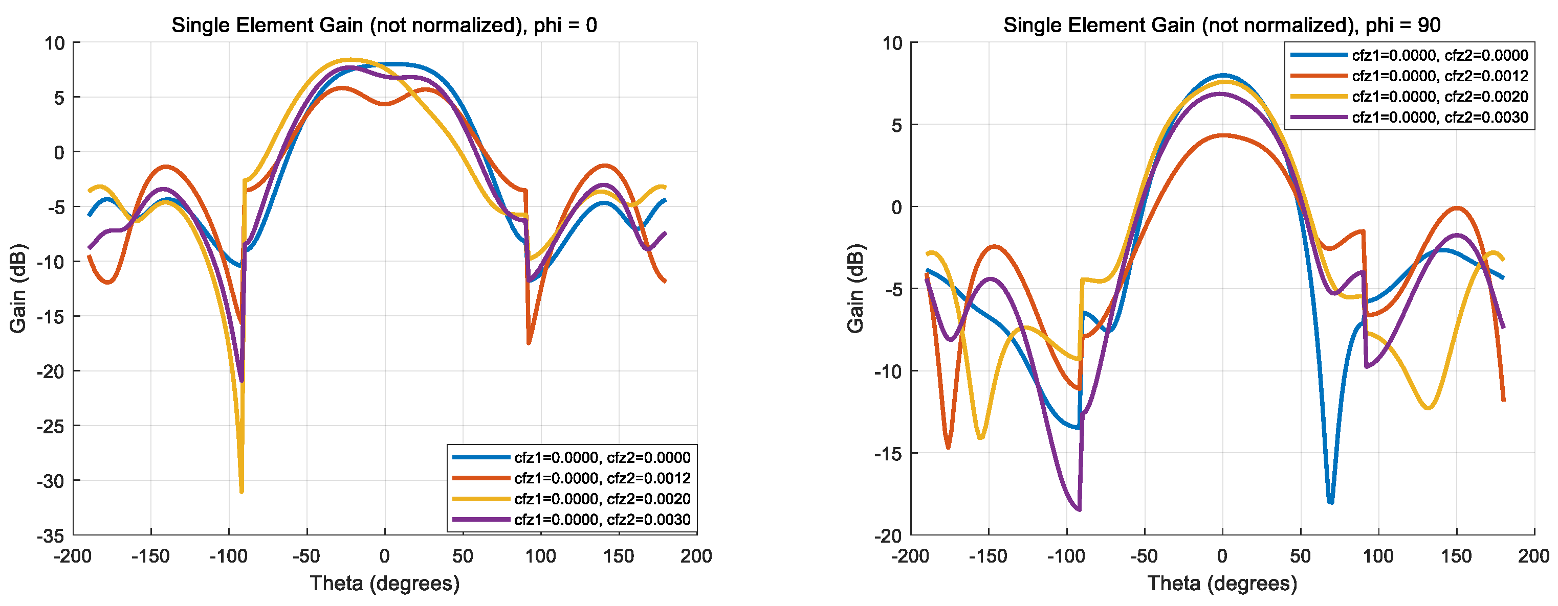
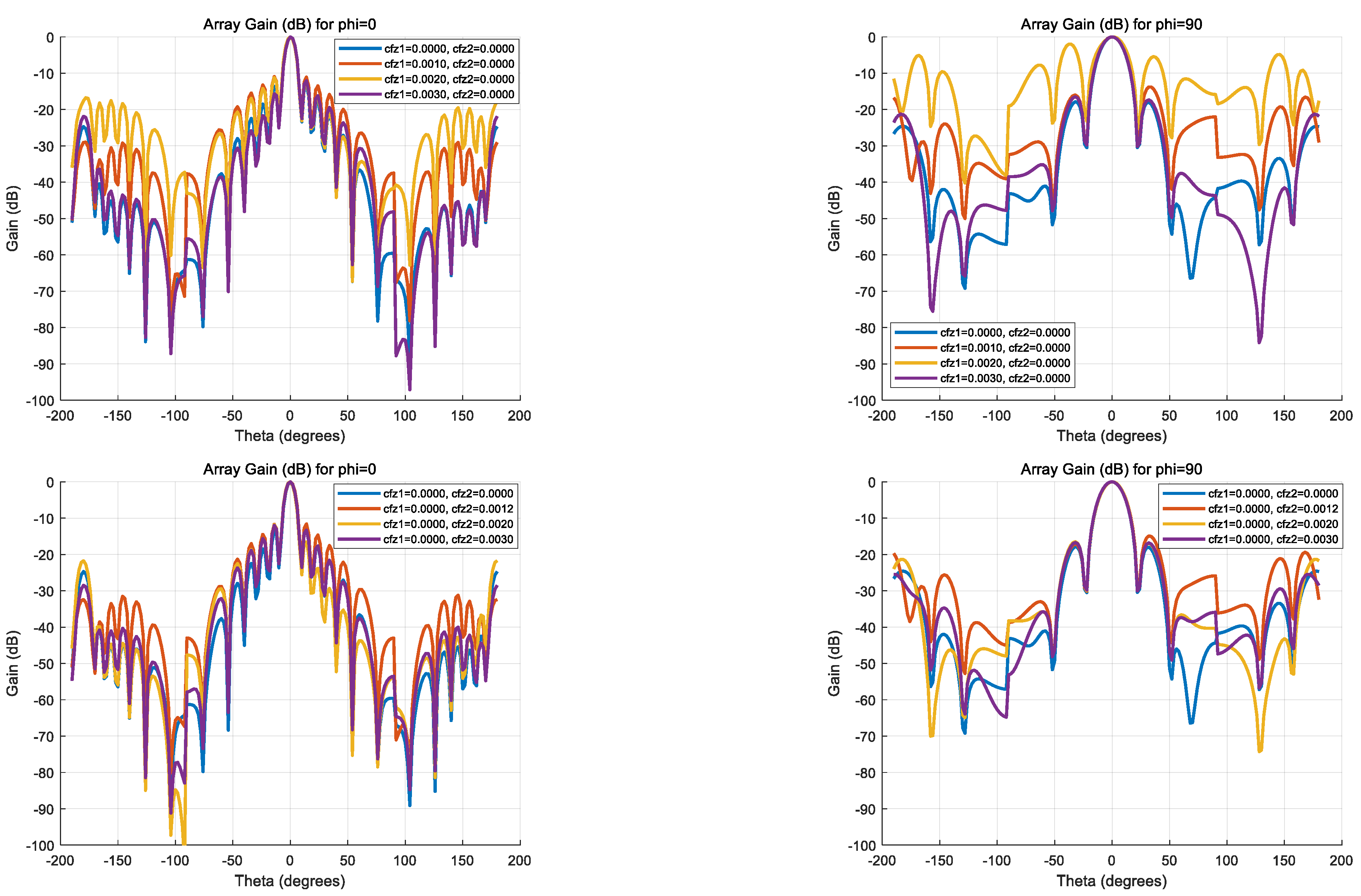
Variations in $c_{fz1}$ and $c_{fz2}$ lead to significant changes in membrane surface accuracy, which, in turn, affect the peak gain and sidelobe structure. Excessive structural modification in either parameter can degrade beam symmetry and increase sidelobe interference.

(3)

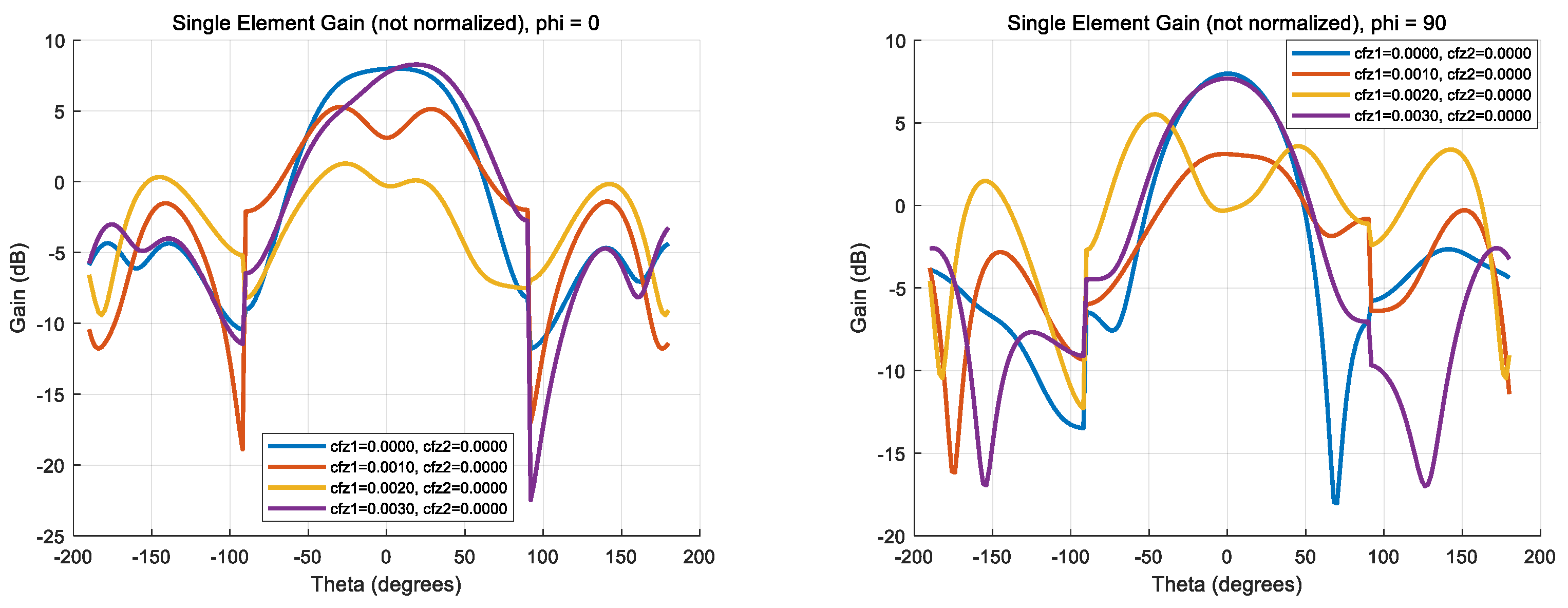
As $c_{fz2}$ increases (e.g., reaching 0.30), the main lobe gain decreases, and sidelobes intensify, indicating potential degradation in directional performance and an increased risk of interference.

(4)

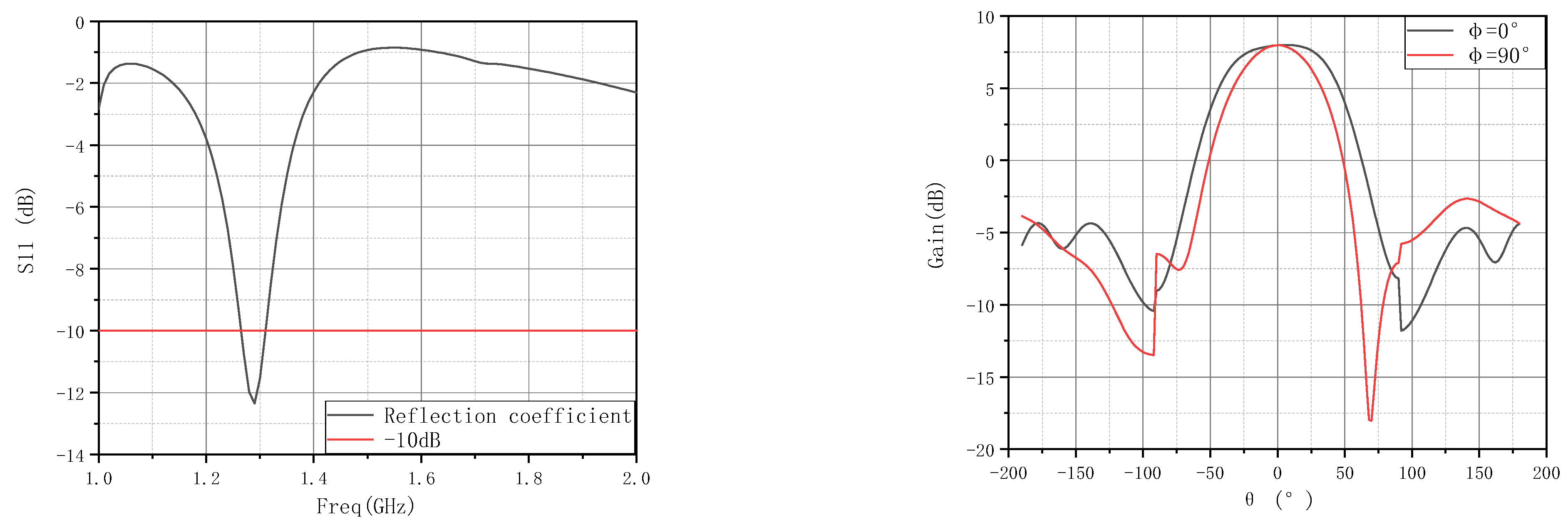
S-parameter analysis reveals that increasing $c_{fz1}$ and $c_{fz2}$ causes resonant frequency shifts and impedance mismatches. Notably, at $c_{fz2}$ = 0.30, the return loss significantly worsens, potentially compromising the antenna’s operational efficiency at 1.3 GHz.

(5)

Phased array simulations show that while the antenna maintains high gain at broadside (θ ≈ 0°), its radiation pattern becomes increasingly distorted at larger $c_{fz2}$ values. In particular, gain symmetry is preserved at φ = 0°, but deformation is more pronounced at φ = 90°, demonstrating directional sensitivity to the structural design.

In summary, this work provides a structural–electromagnetic co-simulation framework based on $c_{fz1}$ and $c_{fz2}$ parameterization, enabling rapid assessment of how structural design influences wrinkling, impedance, and radiation pattern. These findings offer valuable theoretical and simulation guidance for future design and optimization of thin-film phased array antennas.

References

- Ma, X.; Li, J.; Ma, J.; Wang, Z.; Shi, C.; Zheng, S.; Cui, Q.; Li, X.; Liu, F.; Guo, H.; et al. China’s Space Deployable Structures: Progress and Trends. Engineering 2020, 17, 207–219. [Google Scholar] [CrossRef]
- Ma, X.; An, N.; Cong, Q.; Bai, J.B.; Wu, M.; Xu, Y.; Jia, Q. Design, modeling, and manufacturing of high strain composites for space deployable structures. Commun. Eng. 2024, 3, 78. [Google Scholar] [CrossRef]
- Duan, B. Large spaceborne deployable antennas (LSDAs)—A comprehensive summary. Chin. J. Electron. 2020, 29, 1–15. [Google Scholar] [CrossRef]
- Liu, Z.Q.; Qiu, H.; Li, X.; Yang, S.L. Review of large spacecraft deployable membrane antenna structures. Chin. J. Mech. Eng. 2017, 30, 1447–1459. [Google Scholar] [CrossRef]
- Zhou, X.; Ma, X.; Li, H. Research status and development trends of flexible tensioned thin-film deployable space antennas. China Space Sci. Technol. 2022, 42, 15. (In Chinese) [Google Scholar]
- Shinde, S.D.; Upadhyay, S.H. Investigation on effect of tension forces on inflatable torus for rectangular multi-layer planar membrane reflector. Mater. Today Proc. 2023, 72, 1486–1489. [Google Scholar] [CrossRef]
- Li, M.J.; Li, M.; Liu, Y.F.; Geng, X.Y.; Li, Y.Y. A review on the development of spaceborne membrane antennas. Space Sci. Technol. 2022, 2022, 1–12. [Google Scholar] [CrossRef]
- Landis, C.M.; Huang, R.; Hutchinson, J.W. Formation of surface wrinkles and creases in constrained dielectric elastomers subject to electromechanical loading. J. Mech. Phys. Solids 2022, 167, 105023. [Google Scholar] [CrossRef]
- Mierunalan, S.; Dassanayake, S.P.; Mallikarachchi, H.M.Y.C.; Upadhyay, S.H. Simulation of ultra-thin membranes with creases. Int. J. Mech. Mater. Des. 2022, 19, 73–94. [Google Scholar] [CrossRef]
- Hakim, G.; Abramovich, H. Large deflections of thin-walled plates under transverse loading: Investigation of the generated in-plane stresses. Materials 2022, 15, 1577. [Google Scholar] [CrossRef]
- Yang, P.; Fang, Y.; Yuan, Y.; Meng, S.; Nan, Z.; Xu, H.; Gao, H. A perturbation force based approach to creasing instability in soft materials under general loading conditions. J. Mech. Phys. Solids 2021, 151, 104401. [Google Scholar] [CrossRef]
- Zhang, J.; Qiu, X.; Wang, C.; Liu, Y. A general theory and analytical solutions for post-buckling behaviors of thin sheets. J. Appl. Mech. 2022, 89, 061003. [Google Scholar] [CrossRef]
- Pamulaparthi Venkata, S.; Balbi, V.; Destrade, M.; Zurlo, G. Designing necks and wrinkles in inflated auxetic membranes. Int. J. Mech. Sci. 2024, 268, 109031. [Google Scholar] [CrossRef]
- Hao, Y.K.; Li, B.; Feng, X.Q.; Gao, H. Wrinkling–dewrinkling transitions in stretched soft spherical shells. Int. J. Solids Struct. 2024, 294, 112773. [Google Scholar] [CrossRef]
- Rammane, M.; Elmhaia, O.; Mesmoudi, S.; Askour, O.; Braikat, B.; Tri, A.; Damil, N. On the use of Hermit-type WLS approximation in a high order continuation method for buckling and wrinkling analysis of von-Kàrmàn plates. Eng. Struct. 2023, 278, 115498. [Google Scholar] [CrossRef]
- Yan, D.; Huangfu, D.; Zhang, K.; Hu, G. Wrinkling of the membrane with square rigid elements. EPL (Europhys. Lett.) 2016, 116, 24005. [Google Scholar] [CrossRef]
- Zhang, S.Q.; Lai, W.J.; Huang, C.Y.; Cai, C.S.; Lin, C.H.; Zhu, Q.H. Dynamic modeling and control of rigid-flexible-thermo-electrically coupled piezoelectric integrated smart spacecraft. Appl. Math. Model. 2025, 140, 115896. [Google Scholar] [CrossRef]
- Li, N.; Duan, B.; Zheng, F. Effect of the random error on the radiation characteristic of the reflector antenna based on two-dimensional fractal. Int. J. Antennas Propag. 2012, 2012, 543462. [Google Scholar] [CrossRef]
- Yu, D.; Yang, Y.; Hu, G.; Zhou, Y.; Hong, J. Energy harvesting from thermally induced vibrations of antenna panels. Int. J. Mech. Sci. 2022, 231, 107565. [Google Scholar] [CrossRef]
- Li, H.; Lyu, S.; Ma, X.; Lin, K.; Zhang, D.; Zhou, X.; Jin, X. Topology design of modular unit and cable network of on-orbit modular-assembled antenna. Int. J. Aerosp. Eng. 2024, 2024, 6385683. [Google Scholar] [CrossRef]
- Xu, P.; Wang, Y.; Xu, X.; Wang, L.; Wang, Z.; Yu, K.; Wang, C. Structural-electromagnetic-thermal coupling technology for active phased array antenna. Int. J. Antennas Propag. 2023, 2023, 2843443. [Google Scholar] [CrossRef]
- Jia, Y.; Wei, X.; Xu, L.; Wang, C.; Lian, P.; Xue, S.; Shi, Y. Multiphysics vibration FE model of piezoelectric macro fibre composite on carbon fibre composite structures. Compos. Part B Eng. 2019, 161, 376–385. [Google Scholar] [CrossRef]
- Wang, C.; Wang, Y.; Zhou, J.; Wang, M.; Zhong, J.; Duan, B. Compensation method for distorted planar array antennas based on structural–electromagnetic coupling and fast Fourier transform. IET Microw. Antennas Propag. 2018, 12, 954–962. [Google Scholar] [CrossRef]
- Zhang, S.; Zhang, Y.; Yang, D.; Song, L.; Zhang, X. Second-order sensitivity analysis of electromagnetic performance with respect to surface nodal displacements for reflector antennas and its benefits in integrated structural–electromagnetic optimisation. IET Microw. Antennas Propag. 2017, 11, 1530–1535. [Google Scholar] [CrossRef]
- Zeb, B.A.; Afzal, M.U.; Esselle, K.P. Performance analysis of classical and phase-corrected electromagnetic band gap resonator antennas with all-dielectric superstructures. IET Microw. Antennas Propag. 2016, 10, 1276–1284. [Google Scholar] [CrossRef]
- Hadarig, R.C.; de Cos, M.E.; Las-Heras, F. High-performance computational electromagnetic methods applied to the design of patch antenna with EBG structure. Int. J. Antennas Propag. 2012, 2012, 435890. [Google Scholar] [CrossRef]
- Zhou, X.; Li, H.; Ma, X. Analysis of structural boundary effects of copper-coated films and their application to space antennas. Coatings 2023, 13, 1612. [Google Scholar] [CrossRef]
- Balanis, C.A. Antenna Theory: Analysis and Design, 3rd ed.; Wiley: New York, NY, USA, 2005. [Google Scholar]
- Manteghi, M. Analytical Calculation of Impedance Matching for Probe-Fed Microstrip Patch Antennas. IEEE Trans. Antennas Propag. 2009, 57, 3972–3975. [Google Scholar] [CrossRef]
- Mohammed, A.S.B.; Yauri, A.R.; Kabir, A.M. Review of feeding techniques for microstrip patch antenna. Int. J. Comput. Appl. 2019, 178, 97–887. [Google Scholar]