Adaptive Neural Network-Based Fixed-Time Trajectory Tracking Control of Space Robot with Uncertainties and Input Nonlinearities

Abstract

In this paper, a fixed-time control strategy based on neural networks is proposed for a space robot with an input dead zone. First, a model-based control method is proposed based on the fixed-time convergence framework. Due to internal errors and external environmental disturbances, the inertial parameters of dynamic models generally exhibit uncertainties, and model-based control methods may exhibit deviations in trajectory tracking. In order to counteract the adverse effects of uncertain inertial parameters on the system and ensure the stability of the control system, an adaptive learning control method based on neural networks is further proposed. To enhance the learning rate of neural networks and achieve the convergence of neural weights within a fixed time, a neural network update rate combined with virtual control rate is proposed. In addition, considering the issue of the joint input dead zone affecting the precision and stability of the space robot, a novel adaptive law is proposed in conjunction with system error signal feedback to mitigate adverse effects. According to the Lyapunov stability theory, the stability of the closed-loop system is proven, with the trajectory tracking error converging to a small neighborhood around zero. Finally, numerical simulation results demonstrate the effectiveness of the control algorithm.

1. Introduction

With the growing urgency of on-orbit servicing for space devices, the space robot has become a focal point of research for major aerospace powers worldwide. The space-based manipulator, as one of the pivotal technologies in the aerospace field, plays a crucial role in on-orbit services such as the assembly, maintenance, and refueling of spacecraft [1,2,3]. The assembly, construction, maintenance, and application of the International Space Station have demonstrated that utilizing a space robot can assist or substitute astronauts in executing on-orbit operations under harsh conditions. Such tasks include maintaining and repairing malfunctioning spacecraft or satellites, replenishing fuel for space vehicles, and retrieving discarded launch objects [4,5]. This approach enhances efficiency, safety, and reduces the overall cost and risk associated with space exploration. In the microgravity environment of space, the base spacecraft exhibits non-fixed characteristics, leading to strong coupling between the manipulator and the base spacecraft. That is, the motion of the manipulator will, in turn, affect the motion state of the base spacecraft, causing pose disturbances to the base, which in turn impacts the accuracy and stability of the control, posing challenges to the design of the control system [6,7,8]. Therefore, the control of the space manipulator has attracted significant attention [9,10,11].

Given the importance of the space manipulator, precise control of them has been a focal research area for scholars [12,13]. In the control process of space manipulators, due to the limitations imposed by the operating time window, dynamic response, and workspace, the operational tasks must be completed within a fixed-time while ensuring that the end-effector meets physical constraints [14,15]. A fixed-time control strategy, addressing the aforementioned challenges and difficulties, has been proposed and implemented. Compared to traditional asymptotic convergence, fixed-time control offers faster convergence rates and enhanced robustness, ensuring that the system stabilizes within a fixed-time. In [16], for flexible air-breathing hypersonic vehicles operating under actuator saturation conditions, a robust fixed-time control technique featuring adaptive anti-saturation capabilities has been developed. To ensure the tracking error of the autonomous robotic manipulator converges within a fixed time, Ref. [17] introduces a unique globally integral terminal sliding mode surface. In [18], a nonlinear fixed-time H∞ controller was devised utilizing the backstepping method. Ref. [19] introduced a dual-arm humanoid space manipulator that employs a fixed-time state-dependent Riccati equation controller for regulating free flight.

Although fixed-time control algorithms have been successively developed and applied due to their advantages, the convergence time of trajectory tracking errors in fixed-time control is significantly dependent on the initial conditions of the system. This implies that the convergence time of the system state cannot be guaranteed when the initial condition values are not in the ideal state. In practical operating conditions, the initial states of the system are often complex and variable, which leads to the limitations of fixed-time control algorithms. Based on the research of fixed-time control, the fixed-time theory has been further proposed. Compared to traditional fixed-time control methods, fixed-time control overcomes the limitation of initial parameter values, does not rely on the initial state of the system, and provides a faster transition process and higher steady-state accuracy. In [20], an adaptive non-singular sliding-mode control system with a fixed-time under saturated actuator conditions is presented. Fixed-time sliding mode control was developed in [21] based on fixed-time sliding surfaces and fixed-time arrival strategies. In [22], the task-space tracking control problem of a free-floating space robot is tackled using a fixed-time control strategy, which is based on an extended state observer. In [23], fixed-time controllers and fixed-time perturbation observers are proposed simultaneously for fault-tolerant attitude tracking control of spacecraft, incorporating event-triggered mechanisms to enable autonomous spacecraft rendezvous and docking missions. In [24], an adaptive fixed-time controller, featuring seamless transitions between fractional and quadratic form feedback, is developed.

In the research of fixed-time convergence, linear systems predominantly garner attention. However, the space robot, as a prototypical nonlinear system, confronts the challenge of unavailable or inaccurate actual parameter values, complicating precise control and diminishing tracking performance. In addition, due to the interference of harsh environmental factors in space, uncertainty may exist in the model of the space robot. To address the issue of dynamic model uncertainty in nonlinear systems, neural networks have garnered significant attention from numerous scholars. Among them, the radial basis function neural network (RBFNN) stands out due to its straightforward structure, high fitting efficiency, exceptional nonlinear approximation capabilities, and advanced global approximation capabilities. It excellently compensates for unknown elements within dynamical models, making it one of the most commonly used methods for addressing nonlinear control model uncertainties. Ref. [25] investigated an end-to-end neural network controller for optimal control of a quadcopter. Ref. [26] proposed an adaptive neural network force tracking impedance control scheme based on a nonlinear observer. In Ref. [27], an adaptive law is proposed to estimate the local upper bounds of the subsystems of a non-complete mobile robot, based on the developed robust adaptive neural network tracking controller. In [28], for a flexible-joint free-floating space robot vibration suppression control orientated on error models, a reliable control technique based on an adaptive neural network is suggested. Ref. [29] use an acceleration feedback-based RBFNN control technique to stifle self-excited vibration and ensure position precision. A general motion planning framework based on deep reinforcement learning and artificial neural networks is proposed in [30] for a robot with arbitrary geometry. Ref. [31] investigates the neural network-based control problem for robotic systems with error constraints. Ref. [32] developed a nonsingular fixed-time adaptive neural control scheme via backstepping technique for a free-flying flexible-joint space robot when capturing a space target with unknown mass. Given the unique advantages of neural networks in approximating nonlinearities quickly and with high fitting efficiency, this paper eliminates the nonlinear effects of the space robot by designing a radial basis function neural network. Furthermore, compared to the traditional radial basis function neural network, the proposed update rate enhances the learning rate and iteration efficiency of the neural network.

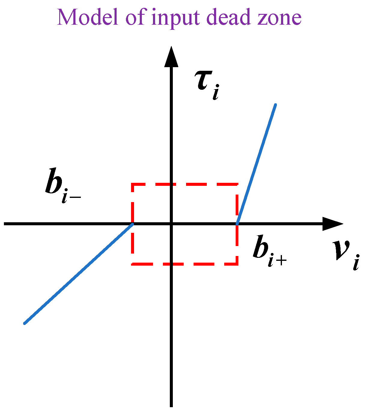
In space robots, joint dead zone characteristics are very common due to friction between the joints and the lack of sensitivity of sensors and actuators to subtle signals. The meaning of dead zone characteristics is that, until the input torque of the joint reaches the boundary value of the dead zone, the system’s output torque remains zero. In the control process of the space robot, the dead zone is a significant factor affecting the precision and stability of the control system and cannot be overlooked. Dead zone phenomena are commonly observed in the control systems of space robot actuators, where most of these phenomena are unpredictable and sporadically changing, exerting a profound impact on control precision, potentially causing system control failure and ultimately leading to the inability of the space robot to complete its space mission. Ref. [33] address the matter through the design of a compensator aimed at mitigating the impacts of uncertain non-linear systems characterized by dead zone input nonlinearities and unspecified dead zone parameters. Ref. [34] introduce converting the dead zone model into a nonlinear model that can be approximated by a fuzzy logic system to mitigate the impacts of the dead zone. In [35], the backstepping method and the obstacle Lyapunov function are used to examine an uncertain manipulator with complete state restrictions and input dead zone. In the presence of external disturbances and parameter uncertainties, Ref. [36] discusses the effects of a non-smooth dead zone during spacecraft attitude tracking operations. Inspired by the appeal work, the effect of the input dead zone on the space manipulator model must be fully considered during the system control process. Inspired by the aforementioned work, the impact of joint torque input dead zone on the space robot model must be fully considered during the system control process. Inadequate handling of a joint torque input dead zone may not only increase tracking errors but also cause limit oscillations in the system, leading to performance degradation or instability, thereby preventing the completion of pre-assigned tasks [37,38].

Based on the preceding discussion, the topics of fixed-time control, neural network compensation for uncertainties, and input dead zone remain pivotal in the field of space robot control, with substantial openness for further research. In [39,40,41], although these situations were considered simultaneously, they were not space robots, and their methods do not account for the microgravity environment, kinematic redundancy, and contact uncertainty inherent to space robots. This paper proposes a fixed-time control strategy based on neural networks for space robotic systems with an input dead zone. By integrating fixed-time convergence into the design of model-based and neural network control methods, a new neural network update rate is proposed, which enhances the learning rate of the neural network and ensures the convergence of the neural network weights within a fixed time. Considering joint input dead zone issues affecting the precision and stability of space robots, a new adaptive law is designed by integrating system error feedback and neural networks into the controller to compensate. By using the Lyapunov stability theory, the stability of the closed-loop system is proved, with trajectory tracking errors and the neural network weights converging to a small region near zero. This control strategy not only compensates for the system’s uncertain terms, ensuring convergence within fixed time, but also eliminates the destabilizing effects of the joint input dead zone. A comparison with traditional PD and SMC controllers reveals that the proposed control algorithm demonstrates superior trajectory tracking performance, validating the effectiveness of the control algorithm.

The main contributions of this paper are as follows:

(1)

For a space robot with an input dead zone, a fixed-time control algorithm based on neural networks was proposed on the basis of model-based control algorithms. This algorithm ensures the rapid tracking of desired trajectories by the manipulator and converges the error to a small neighborhood of zero within a fixed time.

(2)

The proposed neural network update rate ensures the convergence of the neural network weights within a fixed time, handles uncertain system inertia parameters, and simultaneously enhances the learning rate of the neural network.

(3)

A novel adaptive law was designed to compensate for an input dead zone based on feedback from the system’s error signal, thereby enhancing both the accuracy and stability of the system.

2. Dynamics Modeling

2.1. Space Manipulator Model

Figure 1 illustrates an n-link space manipulator system. By applying the law of momentum conservation of the system and the second kind of Lagrange equations, the dynamic equations governing the position and orientation of the payload, both of which are uncontrollable, can be derived [6]:

$$D(q)\ddot{q}+H(q,\dot{q})\dot{q}=\tau ,$$

(1)

In the aforementioned expressions, $\mathit{q}\in [\hspace{0.17em}{q}_1,\hspace{0.17em}{q}_2,\hspace{0.17em}{q}_3,\hspace{0.17em}\dots ,\hspace{0.17em}{q}_n]\in {\mathit{R}}^n$ represents the space manipulator’s generalized position, which takes into account the spacecraft base’s attitude and the manipulator’s joint angles, $\dot{\mathit{q}}$ and $\ddot{\mathit{q}}$ represent the first and second order derivatives of $\mathit{q}$ with respect to time. $\mathit{D}(\mathit{q})\in {\mathit{R}}^{n\times n}$ represents the symmetric positive definite mass matrix, $\mathit{H}(\mathit{q},\dot{\mathit{q}})\dot{\mathit{q}}\in {\mathit{R}}^{n\times n}$ is a column vector incorporating Coriolis and centrifugal forces, and $\mathit{\tau }\in [{\tau }_1,\hspace{0.17em}{\tau }_2,\hspace{0.17em}{\tau }_3,\hspace{0.17em}\dots ,\hspace{0.17em}{\tau }_n]\in {\mathit{R}}^n$ is the output column vector of the actuator torques at the two joints after passing through the dead zone. Details are provided in Appendix A.

2.2. Joint Torque Dead Zone Input Model

“Dead zone” refers to the relationship between input and output in a joint where the output remains zero until the input magnitude reaches a certain threshold. From the perspective of feedback control, the dead zone can be considered as a form of information loss. This paper contemplates the dead zone model illustrated in Figure 2, and the nonlinear description of the dead zone is expressed as where the input dead zone is denoted by $\mathit{v}\in {[\begin{array}{ccc}{v}_1& v_2& v_3\end{array}]}^T$ and the output by $\mathit{\tau }\in {[\begin{array}{ccc}{\tau }_1& {\tau }_2& {\tau }_3\end{array}]}^T$. The nonlinear description of the dead zone is expressed as [33]

$${\mathit{\tau }}_i=\left\{\begin{array}{l}{h}_{ri}(v_i-b_{i+}),\hspace{0.17em}\hspace{0.17em}\hspace{0.17em}\hspace{0.17em}\hspace{0.17em}\hspace{0.17em}v\ge b_{i+}\hfill \\ 0,\hspace{0.17em}\hspace{0.17em}\hspace{0.17em}\hspace{0.17em}\hspace{0.17em}\hspace{0.17em}\hspace{0.17em}\hspace{0.17em}\hspace{0.17em}\hspace{0.17em}\hspace{0.17em}\hspace{0.17em}\hspace{0.17em}\hspace{0.17em}\hspace{0.17em}\hspace{0.17em}\hspace{0.17em}{b}_{i-}<v<b_{r+}\hfill \\ h_{li}(v_i-b_{i-}),\hspace{0.17em}\hspace{0.17em}\hspace{0.17em}\hspace{0.17em}\hspace{0.17em}v\le b_{i-}\hfill \end{array}\right.,$$

(2)

In the equation, $b_{i+}$ and $b_{i-}$ are the left and right breakpoints of the dead zone, and $h_{ri}$ and $h_{li}$ are the left and right slopes of the dead zone. The above dead zone parameters are all bounded uncertainties. Set $b_{i+}>0$ and $b_{i-}<0$, $b_{i+}=5$, and $b_{i-}=-5$.

2.3. Neural Network Model

Neural networks are a type of computational model inspired by the biological nervous system, utilized in the fields of machine learning and artificial intelligence. It mimics the way information is transmitted between neurons through synaptic connections in the human brain, accomplishing sophisticated data processing and learning tasks via stacked neural networks. Specifically, a neural network consists of multiple layers, including an input layer, hidden layers, and an output layer. Each layer consists of multiple neurons, with each neuron receiving information from neurons in the previous layer or input data, transmitting the processed information to the next layer. The structure of the RBFNN is shown in Figure 3. Neurons convert input signals into output signals through activation functions, thereby performing nonlinear mapping and feature extraction on the input data. The radial basis function neural network (RBFNN) is a three-layer network that exhibits excellent approximation capabilities for a wide range of strongly nonlinear functions, taking the form of:

$$\mathit{f}(\mathit{Z})={\mathit{W}}^T\mathit{S}(\mathit{Z}),$$

(3)

where $\mathit{f}(\mathit{Z})$ represents a nonlinear function, $\mathit{Z}={\left[z_1,z_2,\dots ,z_n\right]}^T\in {\mathit{R}}^n$ denotes the input to the neural network, ${\mathit{W}}_i$ signifies the predetermined neural network weights, and $\mathit{S}(\mathit{Z})={\left[s_1,s_2,\dots ,s_n\right]}^T\in {\mathit{R}}^n$ denotes the collection of Gaussian basis functions. Select $\mathit{q},\dot{\mathit{q}}$ and $\mathit{e},\dot{\mathit{e}}$ as inputs for the neural network. The specific form is given by [29]:

$$s(z_i)=\exp \left[{\displaystyle \frac{-{(z_i-{\sigma }_i)}^T(z_i-{\sigma }_i)}{b^2}}\right],$$

(4)

$\mathit{\sigma }={\left[{\sigma }_1,{\sigma }_2,\dots ,{\sigma }_n\right]}^T\in {\mathit{R}}^n$ represents the Gaussian function’s central value, and $b$ represents the Gaussian function’s radial range width, $b$ is set to 5.

An approximation of the Gaussian function can be expressed as

$$\mathit{f}(\mathit{Z})={\mathit{W}}^{*T}\mathit{S}(\mathit{Z})+\Delta (\mathit{Z}),$$

(5)

$\Delta (\mathit{Z})$ stands for the error, and it is bounded in a compact set, with the weight vector defined as ${\mathit{W}}^{*}$ is:

$${\mathit{W}}^{*}=\arg {\min }_{\mathit{W}\in \mathit{R}}\left\{{\sup }_{\mathit{Z}\in \mathit{R}}\left|\mathit{f}(\mathit{Z})-{\mathit{W}}^T\mathit{S}(\mathit{Z})\right|\right\},$$

(6)

It can be known that ${\mathit{W}}^{*}$ minimizes the error.

Next, we introduce some of the fundamental inequalities in mathematical analysis that will provide the mathematical basis in subsequent stability proofs, helping us limit the interaction of key variables in the system, such as state errors and control inputs, thus avoiding over-confinements while guaranteeing the stability of the algorithm, ensuring that the resulting conclusions hold strictly mathematically.

Lemma 1 

([42]). For $a_1,a_2,\dots ,a_n$ and $x\in R,0\le x\le 1$, the following inequality is present ${(|a_1|+\dots +|a_n|)}^x\le |a_1{|}^x+\dots +|a_n{|}^x$

Lemma 2 

([43]). For $x_k>0,k=1,2,\dots ,n$ , The following inequality holds ${({\displaystyle \sum _{k=1}^n}{x}_k)}^2={({\displaystyle \sum _{k=1}^n}1\cdot x_k)}^2\le n\cdot {\displaystyle \sum _{k=1}^n}{x}_k^2$

Lemma 3 

([44]). For $x,y\in \mathrm{R}$ , the following inequality holds $xy\le {\displaystyle \frac{{\epsilon }^a}{a}}|x{|}^a+{\displaystyle \frac{1}{b{\epsilon }^b}}|y{|}^b$, where $\epsilon >0,a>1,b>1,(a-1)(b-1)=1$

Lemma 4 

([45]). For a general dynamical system  $\dot{x}(t)=f(t,x)$ , $x(0)=x_0$, assume that the origin is an equilibrium point and $x\in {\mathrm{R}}^{\mathrm{n}}$, $f_{+}:\mathrm{R}\times {\mathrm{R}}^{\mathrm{n}}\to \mathrm{R}$. Given a positive definite function $V(x)$, and for some $\alpha ,\beta >0,p>1,0<q<1$, there are $\dot{V}(x)\le -\alpha V^p(x)-\beta V^q(x)$. A time function is a mathematical expression or algorithm that defines how a system’s output or state evolves with respect to time. The origin of the system is stable within a fixed time, where the time function can be set as

$$T_{fd}\le T_{\max }={\displaystyle \frac{1}{\alpha (p-1)}}+{\displaystyle \frac{1}{\beta (1-q)}},$$

(7)

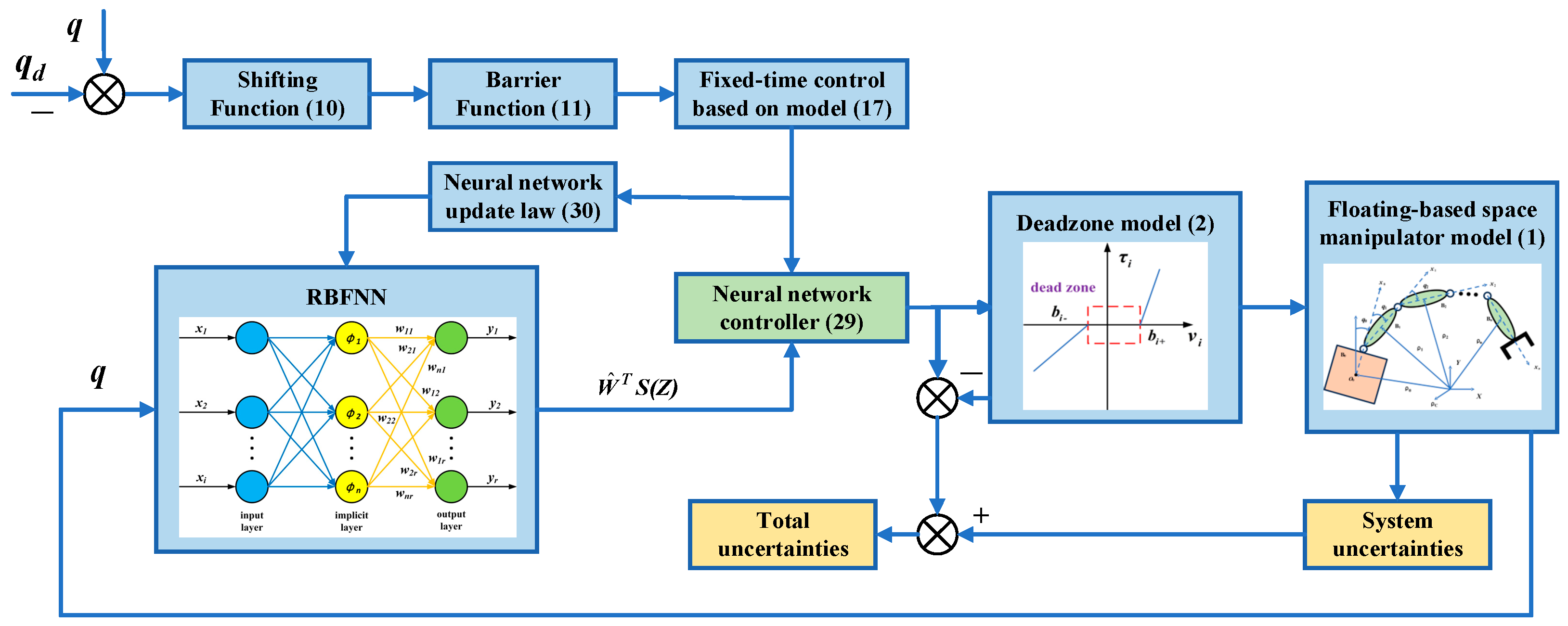
3. Controller Design

For the free-floating base space manipulator system, define ${\mathit{q}}_{\mathit{d}}={\left[q_{d0},q_{d1},q_{d2}\right]}^T$ as the expected trajectory of the system, the tracking error being

$${\mathit{e}}_1=\mathit{q}-{\mathit{q}}_{\mathit{d}},$$

(8)

$${\mathit{e}}_2=\dot{\mathit{q}}-\mathit{\alpha },$$

(9)

$\mathit{\alpha }$ serves as a virtual control law designed for the subsequent sections, and additionally, a time-varying switching function is to be designed as follows:

$${\xi }_i(t)=\left\{\begin{array}{l}{\mathrm{e}}^{-{\displaystyle \frac{{(\tan (\frac{\pi (T_s-t)}{2T_s}))}^{2n}}{2{\sigma }^{2n}}}},\hspace{0.17em}\hspace{0.17em}\hspace{0.17em}\hspace{0.17em}0\le t<T_s\hfill \\ 1,\hspace{0.17em}\hspace{0.17em}\hspace{0.17em}\hspace{0.17em}\hspace{0.17em}\hspace{0.17em}\hspace{0.17em}\hspace{0.17em}\hspace{0.17em}\hspace{0.17em}\hspace{0.17em}\hspace{0.17em}\hspace{0.17em}\hspace{0.17em}\hspace{0.17em}\hspace{0.17em}\hspace{0.17em}\hspace{0.17em}\hspace{0.17em}\hspace{0.17em}\hspace{0.17em}\hspace{0.17em}\hspace{0.17em}\hspace{0.17em}\hspace{0.17em}\hspace{0.17em}{T}_s\le t\hfill \end{array}\right.,$$

(10)

where $\sigma$ is a normal constant, $n$ is the order of the system, $\mathrm{e}$ is the base of the natural logarithm function, and $T_s$ is a custom time.

Let ${\kappa }_i={\xi }_i(t)e_{1i}$ with $e_{1i}$ being the ith element of ${\mathit{e}}_1$, introducing the barrier function:

$${\eta }_i={\displaystyle \frac{{{\rm Y}}_{ui}{{\rm Y}}_{li}{e}_{1i}}{({{\rm Y}}_{li}+{\kappa }_i)({{\rm Y}}_{ui}-{\kappa }_i)}},$$

(11)

where ${{\rm Y}}_{ui}$ and ${{\rm Y}}_{li}$ are positive functions that depend on the time of the bounded variable $e_{1i}$, with ${{\rm Y}}_{li}$ denoting the lower bound and ${{\rm Y}}_{ui}$ denoting the upper bound.

Remark 1. 

If $0\le t\le T_s$, $\sigma$ will establish the rate of convergence of the shift function (11), when $\sigma$ is sufficiently small, as ${\xi }_i(t)$ tends to 1, ${\kappa }_i$ will converge rapidly to $e_{1i}$ . If $t\ge T_s$ , ${\xi }_i(t)=1$ can be obtained through Equation (11), then ${\kappa }_i=e_{1i}$ . Thus, ${\eta }_i\to \pm \infty$ if and only if $e_{1i}\to {{\rm Y}}_{ui}$ or $e_{1i}\to -{{\rm Y}}_{li}$ . If we can prove that ${\eta }_i$ is bounded, then $-{{\rm Y}}_{li}<{\kappa }_i<{{\rm Y}}_{ui},i=1,\dots ,n$ can be guaranteed. This also implies that, by employing the barrier function (11), the originally constrained system is transformed into an unconstrained one. It should further be noted that when $T_s=0\hspace{0.17em}\hspace{0.17em}\mathrm{s}$ is applied, the system transitions to a conventional control type, with constraints imposed at the onset of operation.

Expanding the derivative for a yields

$${\dot{\eta }}_i={\rho }_i{\dot{e}}_{1i}+{\varphi }_i{\dot{\xi }}_i-{ϵ}_i{\dot{{\rm Y}}}_{ui}+{\varsigma }_i{\dot{{\rm Y}}}_{li}$$

(12)

The elements of the above equation are

$$\begin{gathered} {\rho }_i={\displaystyle \frac{{{\rm Y}}_{li}{{\rm Y}}_{ui}({{\rm Y}}_{li}{{\rm Y}}_{ui}+{\kappa }_i^2)}{{({{\rm Y}}_{li}+{\kappa }_i)}^2{({{\rm Y}}_{ui}-{\kappa }_i)}^2}}, {\varphi }_i=-{\displaystyle \frac{{{\rm Y}}_{li}{{\rm Y}}_{ui}{e}_{1i}^2({{\rm Y}}_{ui}-{{\rm Y}}_{li}-2{\kappa }_i)}{{({{\rm Y}}_{li}+{\kappa }_i)}^2{({{\rm Y}}_{ui}-{\kappa }_i)}^2}} \\ {ϵ}_i={\displaystyle \frac{{{\rm Y}}_{li}{\kappa }_i{e}_{1i}({{\rm Y}}_{li}+{\kappa }_i)}{{({{\rm Y}}_{li}+{\kappa }_i)}^2{({{\rm Y}}_{ui}-{\kappa }_i)}^2}}, {\varsigma }_i={\displaystyle \frac{{{\rm Y}}_{ui}{\kappa }_i{e}_{1i}({{\rm Y}}_{ui}-{\kappa }_i)}{{({{\rm Y}}_{li}+{\kappa }_i)}^2{({{\rm Y}}_{ui}-{\kappa }_i)}^2}} \end{gathered}$$

3.1. Model-Based Fixed-Time Control

Substituting (8) into the above Equation (12), we obtain

$$\dot{\mathit{\eta }}=\mathit{\rho }\dot{\mathit{q}}-\mathit{\rho }{\dot{\mathit{q}}}_{\mathit{d}}+\mathit{\varphi }\dot{\mathit{\xi }}-\mathit{ϵ}{\dot{\mathit{{\rm Y}}}}_{\mathit{u}}+\mathit{\varsigma }{\dot{\mathit{{\rm Y}}}}_{\mathit{l}},$$

(13)

Bringing (9) into the above equation yields, $\mathit{\alpha }$ is the virtual control law designed in (17), which can be obtained as

$$\dot{\mathit{\eta }}=\mathit{\rho }{\mathit{e}}_2+\mathit{\rho }\mathit{\alpha }-\mathit{\rho }{\dot{\mathit{q}}}_{\mathit{d}}-\mathit{\varphi }\dot{\mathit{\xi }}-\mathit{ϵ}{\dot{\mathit{{\rm Y}}}}_{\mathit{u}}+\varsigma {\dot{\mathit{{\rm Y}}}}_{\mathit{l}},$$

(14)

Constructing the Lyapunov function candidate

$$V_1={\displaystyle \frac{1}{2}}{\mathit{\eta }}^T\mathit{\eta },$$

(15)

Then, calculating the time derivative of $V_1$, ${\dot{V}}_1={\mathit{\eta }}^T\mathit{\eta }$, therefore

$${\dot{V}}_1={\mathit{\eta }}^T(\mathit{\rho }{\mathit{e}}_2+\mathit{\rho }\mathit{\alpha }-\mathit{\rho }{\dot{\mathit{q}}}_{\mathit{d}}-\mathit{\varphi }\dot{\mathit{\xi }}-\mathit{ϵ}{\dot{\mathit{{\rm Y}}}}_u+\mathit{\varsigma }{\dot{\mathit{{\rm Y}}}}_{\mathit{l}}),$$

(16)

Design the virtual control rate $\mathit{\alpha }$ as

$$\mathit{\alpha }={\mathit{\rho }}^{-1}(-{\mathit{K}}_1{\displaystyle \frac{\mathit{\eta }}{{\mathit{\eta }}^T\mathit{\eta }}}{({\mathit{\eta }}^T\mathit{\eta })}^{{\displaystyle \frac{1}{2}}}-{\mathit{K}}_2\mathit{\eta }{\mathit{\eta }}^T\mathit{\eta }+\mathit{\varphi }\dot{\mathit{\xi }}+\mathit{ϵ}{\dot{\mathit{{\rm Y}}}}_{\mathit{u}}-\mathit{\varsigma }{\dot{\mathit{{\rm Y}}}}_{\mathit{l}})+{\dot{\mathit{q}}}_{\mathit{d}},$$

(17)

where ${\mathit{K}}_1$, ${\mathit{K}}_2$ are positive definite matrices.

Remark 2. 

According to the configuration, there are no singular points in the virtual control rate (17), and for the term ${\displaystyle \frac{\mathit{\eta }}{{\mathit{\eta }}^T\mathit{\eta }}}$, it is necessary to apply a smooth approximation to this function. A normal constant $c$ can be chosen to satisfy condition ${\mathit{\eta }}^T\mathit{\eta }<c$, with adjustments made to the value of $c$ to accommodate the system feedback, thereby achieving optimal results—adjusted to adapt to the system feedback to obtain the best result.

Substituting (17) into (16) yields the desired outcome

$${\dot{V}}_1=-{\mathit{K}}_1{({\mathit{\eta }}^T\mathit{\eta })}^{{\displaystyle \frac{1}{2}}}-{\mathit{K}}_2{({\mathit{\eta }}^T\mathit{\eta })}^2+{\mathit{\eta }}^T\mathit{\rho }{\mathit{e}}_2,$$

(18)

According to (9) and the kinetic (1), it can be obtained that

$${\dot{\mathit{e}}}_2=\ddot{\mathit{q}}-\dot{\mathit{\alpha }}={\mathit{D}}^{-1}(\mathit{\tau }-\mathit{H}{\mathit{x}}_2)-\dot{\mathit{\alpha }}={\mathit{D}}^{-1}(\mathit{\tau }-\mathit{C}{\mathit{x}}_2-\mathit{H}\dot{\mathit{\alpha }}),$$

(19)

The transformed form, which is

$${\mathit{e}}_2^T\mathit{D}\hspace{0.17em}{\dot{\mathit{e}}}_2={\mathit{e}}_2^T(\mathit{\tau }-\mathit{H}{\mathit{x}}_2-\mathit{D}\dot{\mathit{\alpha }}),$$

(20)

Therefore, based on the appeal derivation, the Lyapunov function is then constructed as

$$V_2=V_1+{\displaystyle \frac{1}{2}}{\mathit{e}}_2^T\mathit{D}{\mathit{e}}_2,$$

(21)

Putting (20) into (21) and solving for the derivative, the time derivative of (22) can be obtained as

$${\dot{V}}_2=-{\mathit{K}}_1{({\mathit{\eta }}^T\mathit{\eta })}^{{\displaystyle \frac{1}{2}}}-{\mathit{K}}_2{({\mathit{\eta }}^T\mathit{\eta })}^2+{\displaystyle \frac{1}{2}}{\mathit{e}}_2^T\dot{\mathit{D}}{\mathit{e}}_2+{\mathit{\eta }}^T\mathit{\rho }{\mathit{e}}_2+{\mathit{e}}_2^T(\mathit{\tau }-\mathit{H}{\mathit{x}}_2-\mathit{D}\dot{\mathit{\alpha }}),$$

(22)

According to the literature [44], ${\displaystyle \frac{1}{2}}\dot{\mathit{D}}-2\mathit{H}$ is a matrix with skew symmetry and its definition shows that ${\mathit{e}}_2^T({\displaystyle \frac{1}{2}}\dot{\mathit{D}}-2\mathit{H}){\mathit{e}}_2=0$ holds for ${\mathit{e}}_2\in {\mathit{R}}^n$. Based on this property, the aforementioned equation can be rewritten as

$${\dot{V}}_2=-{\mathit{K}}_1{({\mathit{\eta }}^T\mathit{\eta })}^{{\displaystyle \frac{1}{2}}}-{\mathit{K}}_2{({\mathit{\eta }}^T\mathit{\eta })}^2+{\mathit{\eta }}^T\mathit{\rho }{\mathit{e}}_2+{\mathit{e}}_2^T(\mathit{v}+\mathsf{\Delta }\mathit{u}-\mathit{H}\mathit{\alpha }-\mathit{D}\dot{\mathit{\alpha }}),$$

(23)

where $\mathit{\tau }=\mathit{v}+\mathsf{\Delta }\mathit{u}$, within the fixed-time convergence framework, we can propose control rates.

$$\mathit{\nu }=-{\mathit{\rho }}^T\mathit{\eta }-{\mathit{K}}_3{\mathit{e}}_2{({\mathit{e}}_2^T{\mathit{e}}_2)}^{-{\displaystyle \frac{1}{2}}}-{\mathit{K}}_4{\mathit{e}}_2{\mathit{e}}_2^T{\mathit{e}}_2+\mathit{H}\mathit{\alpha }+\mathit{D}\dot{\mathit{\alpha }}-\mathsf{\Delta }\mathit{u}$$

(24)

where ${\mathit{K}}_3$, ${\mathit{K}}_4$ are positive definite matrices.

Taking the controller (24) into (23), we get

$${\dot{V}}_2=-{\mathit{K}}_1{({\mathit{\eta }}^T\mathit{\eta })}^{{\displaystyle \frac{1}{2}}}-{\mathit{K}}_2{({\mathit{\eta }}^T\mathit{\eta })}^2-{\mathit{K}}_3{({\mathit{e}}_2^T{\mathit{e}}_2)}^{{\displaystyle \frac{1}{2}}}-{\mathit{K}}_4{({\mathit{e}}_2^T{\mathit{e}}_2)}^2,$$

(25)

Let ${\chi }_1=\min ({\lambda }_{\min }({\mathit{K}}_1),{\displaystyle \frac{{\lambda }_{\min }({\mathit{K}}_3)}{\sqrt{{\lambda }_{\max }(\mathit{D})}}})$, ${\chi }_2=\min ({\lambda }_{\min }({\mathit{{\rm K}}}_2),{\displaystyle \frac{{\lambda }_{\min }({\mathit{{\rm K}}}_4)}{{\lambda }_{\max }^2(\mathit{D})}})$, combining Lemma 1 and Lemma 2. yields

$${\dot{V}}_2\le -\sqrt{2}{\chi }_1{V}_2^{{\displaystyle \frac{1}{2}}}-\sqrt{2}{\chi }_2{V}_2^2,$$

(26)

Theorem 1. 

With regard to the space manipulator (1), the proposed controller (24) enables fixed-time convergence of the closed-loop system, where the settling time function satisfies condition

$$T_{fd}\le T_{\max }={\displaystyle \frac{1}{\sqrt{2}{\chi }_2}}+{\displaystyle \frac{2}{\sqrt{2}{\chi }_1}}$$

(27)

Proof. 

From (26), we can assign $\alpha =-\sqrt{2}{\chi }_1$, $p={\displaystyle \frac{1}{2}}$, $\beta =-\sqrt{2}{\chi }_2$, $q=2$, put these values into (7) in Lemma 4, and (27) is proved. □

3.2. Fixed-Time Control Based on Neural Networks

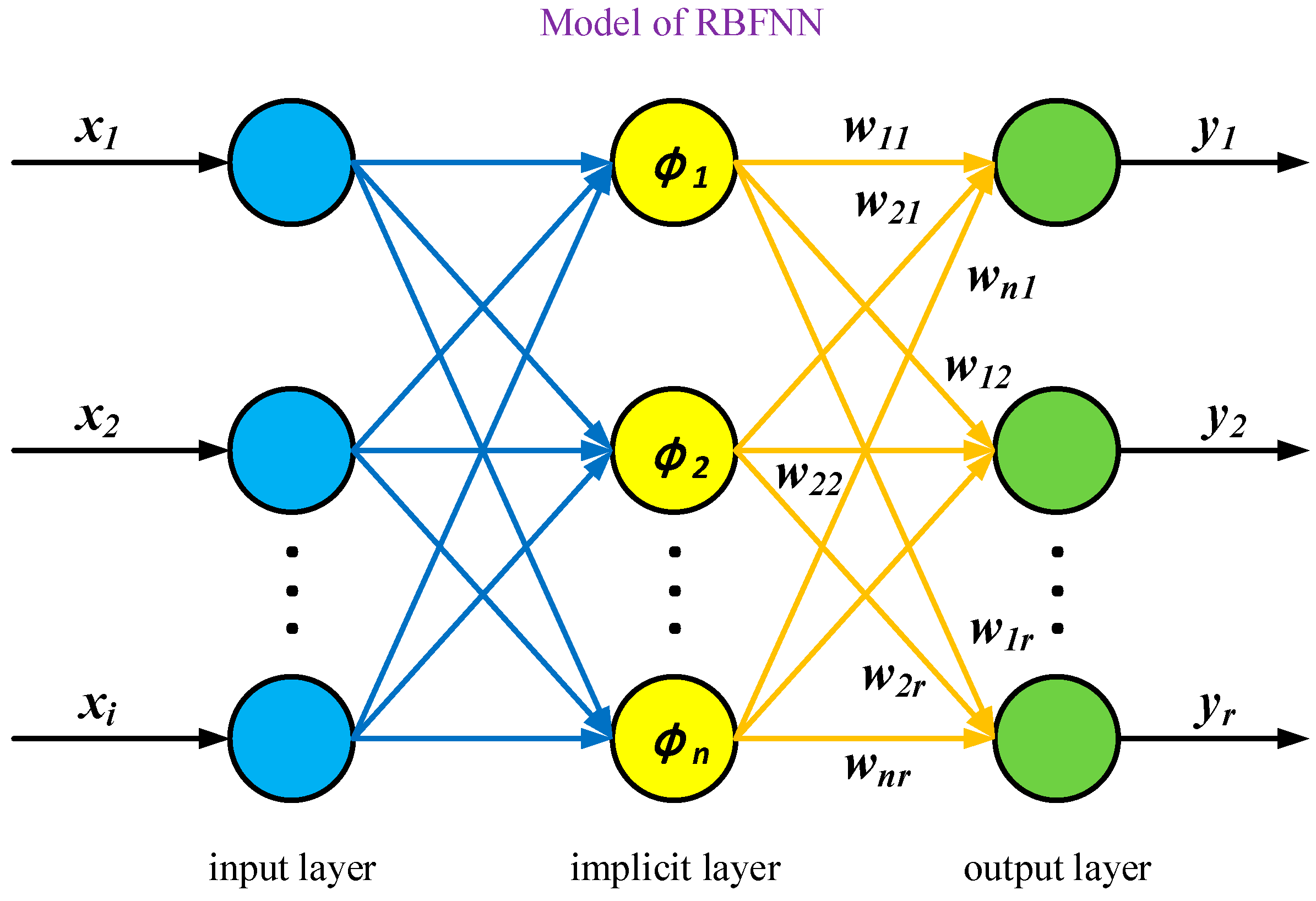
Uncertainty in the model arises from nonlinearities and dead zone effects in the space manipulator, precluding the direct application of the previously mentioned control strategies. Consequently, a neural network is introduced. Neural networks serve as effective tools for addressing model uncertainties, with approximations as shown below:

$${\mathit{W}}^{\ast T}\mathit{S}(\mathit{Z})=\mathit{D}\dot{\mathit{\alpha }}+\mathit{H}\mathit{\alpha }-\mathsf{\Delta }\mathit{u}+ϵ(\mathit{Z})$$

(28)

where $ϵ(\mathit{Z})$ shows the approximate error that satisfies $‖ϵ(\mathit{Z})‖\le \overline{ϵ}$ with $\overline{ϵ}\in R$ and $\overline{ϵ}>0$ which is unknown, $\mathit{Z}={\left[z_1,z_2,\dots ,z_n\right]}^T\in {\mathit{R}}^n$ represents the input of the neural network, ${\mathit{W}}^{\ast }$ denoting the weights of the defined neural network, and $\mathit{S}(\mathit{Z})={\left[s_1,s_2,\dots ,s_n\right]}^T\in {\mathit{R}}^n$ representing the combination of Gaussian basis functions.

Define $\widehat{\mathit{W}}$ as an estimate of ${\mathit{W}}^{\ast }$, $\tilde{\mathit{W}}=\widehat{\mathit{W}}-{\mathit{W}}^{\ast }$. The control rate can be expressed as follows when using the neural network approximation:

$$\mathit{\nu }=-{\mathit{\rho }}^T\mathit{\eta }-{\displaystyle \frac{1}{2}}{\mathit{e}}_2-{\mathit{K}}_3{\mathit{e}}_2{({\mathit{e}}_2^T{\mathit{e}}_2)}^{-{\displaystyle \frac{1}{2}}}\hspace{0.17em}-{\mathit{K}}_4{\mathit{e}}_2{\mathit{e}}_2^T{\mathit{e}}_2\hspace{0.17em}+{\widehat{\mathit{W}}}^T\mathit{S}(\mathit{Z})$$

(29)

The design update rate is $\widehat{\mathit{W}}$:

$$\dot{\widehat{\mathit{W}}}=-\Gamma (\mathit{S}(\mathit{Z}){\mathit{e}}_2+\widehat{\mathit{W}}{\widehat{\mathit{W}}}^T\widehat{\mathit{W}}+\mathit{\sigma }\widehat{\mathit{W}})$$

(30)

$\mathit{\Gamma }\in {\mathit{R}}^{n\times n}$ is a constant gain matrix, the role of the constant gain matrix lies in weighting the gradients of the neural network, facilitating adjustments that accelerate convergence during the weight update process. In certain cases, the gain matrix mitigates issues such as the explosion or disappearance of gradients. $\mathit{\sigma }$ is a positive robustness term; positive robust factors help neural networks control parameter updates during training by providing additional constraints or stability mechanisms. This not only improves the robustness of the model in the face of uncertainty and noise but also helps accelerate convergence and avoid training instability. The diagram of the NNFT controller is shown in Figure 4.

Then, the Lyapunov function is designed as

$$V_3=V_2+\sum _{i=1}^n{\tilde{\mathit{W}}}_i^T{\Gamma }_i^{-1}{\tilde{\mathit{W}}}_i,$$

(31)

Considering (22) and (29), the time derivatives of (31) are

$$\begin{array}{l}{\dot{V}}_3\le -{\mathit{K}}_1{({\mathit{\eta }}^T\mathit{\eta })}^{{\displaystyle \frac{1}{2}}}-{\mathit{K}}_2{({\mathit{\eta }}^T\mathit{\eta })}^2-{\mathit{K}}_3{({\mathit{e}}_2^T{\mathit{e}}_2)}^{{\displaystyle \frac{1}{2}}}-{\mathit{K}}_4{({\mathit{e}}_2^T{\mathit{e}}_2)}^2\\ \hspace{0.17em}\hspace{0.17em}\hspace{0.17em}\hspace{0.17em}\hspace{0.17em}\hspace{0.17em}\hspace{0.17em}\hspace{0.17em}\hspace{0.17em}\hspace{0.17em}-{\displaystyle \frac{1}{2}}{\mathit{e}}_2^T{\mathit{e}}_2+{\mathit{e}}_2^T{\tilde{\mathit{W}}}^T\mathit{S}(\mathit{Z})\hspace{0.17em}+{\mathit{e}}_2^T\mathit{ϵ}(\mathit{Z})+\sum _{i=1}^n{\tilde{\mathit{W}}}_i^T{\Gamma }_i^{-1}{\dot{\widehat{\mathit{W}}}}_i\end{array},$$

(32)

where, ${\mathit{e}}_2^T\mathit{ϵ}(\mathit{Z})\le {\displaystyle \frac{1}{2}}{\mathit{e}}_2^T{\mathit{e}}_2+{\displaystyle \frac{1}{2}}{\overline{ϵ}}^2$, the update rate (30) is brought into (32) to obtain

$$\begin{array}{l}{\dot{V}}_3\le -{\mathit{K}}_1{({\mathit{\eta }}^T\mathit{\eta })}^{{\displaystyle \frac{1}{2}}}-{\mathit{K}}_2{({\mathit{\eta }}^T\mathit{\eta })}^2-{\mathit{K}}_3{({\mathit{e}}_2^T{\mathit{e}}_2)}^{{\displaystyle \frac{1}{2}}}-{\mathit{K}}_4{({\mathit{e}}_2^T{\mathit{e}}_2)}^2\\ \hspace{0.17em}\hspace{0.17em}\hspace{0.17em}\hspace{0.17em}\hspace{0.17em}\hspace{0.17em}\hspace{0.17em}\hspace{0.17em}\hspace{0.17em}\hspace{0.17em}-\sum _{i=1}^n{\tilde{\mathit{W}}}_i^T({\mathit{S}}_i(\mathit{Z})e_{2i}+{\widehat{\mathit{W}}}_i{\widehat{\mathit{W}}}_i^T{\widehat{\mathit{W}}}_i+{\sigma }_i{\widehat{\mathit{W}}}_i)\hspace{0.17em}+{\mathit{e}}_2^T{\tilde{\mathit{W}}}^T\mathit{S}(\mathit{Z})+{\displaystyle \frac{1}{2}}{\overline{ϵ}}^2\end{array},$$

(33)

It is worth noting that ${\mathit{e}}_2^T{\tilde{\mathit{W}}}^T\mathit{S}(\mathit{Z})=\sum _{i=1}^n{\tilde{\mathit{W}}}_i^T{\mathit{S}}_i(\mathit{Z})e_{2i}$.

Therefore, given the equation that will be shown later, first determine a few of its elements:

$$\hspace{0.17em}-{\sigma }_i{\tilde{\mathit{W}}}_i^T{\widehat{\mathit{W}}}_i=-{\sigma }_i{\tilde{\mathit{W}}}_i^T{\tilde{\mathit{W}}}_i-{\sigma }_i{\tilde{\mathit{W}}}_i^T{\mathit{W}}_i^{\ast }\le -{\displaystyle \frac{{\sigma }_i}{2}}{\tilde{\mathit{W}}}_i^T{\tilde{\mathit{W}}}_i+{\displaystyle \frac{{\sigma }_i}{2}}{\mathit{W}}_i^{\ast T}{\mathit{W}}_i^{\ast }\hspace{0.17em}\le -{\sigma }_i{({\tilde{\mathit{W}}}_i^T{\tilde{\mathit{W}}}_i)}^{{\displaystyle \frac{1}{2}}}+{\displaystyle \frac{{\sigma }_i}{2}}({\mathit{W}}_i^{\ast T}{\mathit{W}}_i^{\ast }+1)$$

${\tilde{\mathit{W}}}_i^T{\widehat{\mathit{W}}}_i{\widehat{\mathit{W}}}_i^T{\widehat{\mathit{W}}}_i$ can be broken down into

$$\begin{array}{l}{\tilde{\mathit{W}}}_i^T{\widehat{\mathit{W}}}_i{\widehat{\mathit{W}}}_i^T{\widehat{\mathit{W}}}_i=-\parallel {\tilde{\mathit{W}}}_i{\parallel }^4\hspace{0.17em}-\hspace{0.17em}\parallel {\mathit{W}}_i^{\ast }{\parallel }^2(\parallel {\tilde{\mathit{W}}}_i{\parallel }^2+{\tilde{\mathit{W}}}_i^T{\mathit{W}}_i^{\ast })\\ \hspace{0.17em}\hspace{0.17em}\hspace{0.17em}\hspace{0.17em}\hspace{0.17em}\hspace{0.17em}\hspace{0.17em}\hspace{0.17em}\hspace{0.17em}\hspace{0.17em}\hspace{0.17em}\hspace{0.17em}\hspace{0.17em}\hspace{0.17em}\hspace{0.17em}\hspace{0.17em}\hspace{0.17em}\hspace{0.17em}\hspace{0.17em}-3\parallel {\tilde{\mathit{W}}}_i{\parallel }^2{\tilde{\mathit{W}}}_i^T{\mathit{W}}_i^{\ast }-2\parallel {\tilde{\mathit{W}}}_i^T{\mathit{W}}_i^{\ast }{\parallel }^2\end{array}$$

(34)

According to Lemma 3, it can be obtained that

$$\begin{array}{l}-3\parallel {\tilde{\mathit{W}}}_i{\parallel }^2{\tilde{\mathit{W}}}_i^T{\mathit{W}}_i^{\ast }\le 3\parallel {\tilde{\mathit{W}}}_i{\parallel }^3\parallel {\mathit{W}}_i^{\ast }\parallel \le 3({\displaystyle \frac{3}{4}}{\kappa }_{1i}^{{\displaystyle \frac{4}{3}}}{(\parallel {\tilde{\mathit{W}}}_i{\parallel }^3)}^{{\displaystyle \frac{4}{3}}}+{\displaystyle \frac{1}{4{\kappa }_{1i}^4}}\parallel {\mathit{W}}_i^{\ast }{\parallel }^4),\\ -\parallel {\tilde{\mathit{W}}}_i{\parallel }^2{\tilde{\mathit{W}}}_i^T{\mathit{W}}_i^{\ast }\le \parallel {\tilde{\mathit{W}}}_i{\parallel }^3\parallel {\mathit{W}}_i^{\ast }\parallel \le ({\displaystyle \frac{3}{4}}{\kappa }_{1i}^{{\displaystyle \frac{4}{3}}}{(\parallel {\tilde{\mathit{W}}}_i{\parallel }^3)}^{{\displaystyle \frac{4}{3}}}+{\displaystyle \frac{1}{4{\kappa }_{1i}^4}}\parallel {\mathit{W}}_i^{\ast }{\parallel }^4),\\ -\parallel {\mathit{W}}_i^{\ast }{\parallel }^2\parallel {\tilde{\mathit{W}}}_i{\parallel }^2\le -\parallel {\mathit{W}}_i^{\ast }{\parallel }^2(2\parallel {\tilde{\mathit{W}}}_i\parallel -1)\end{array}$$

where ${\kappa }_{1i}>0$, ${\kappa }_{2i}>0$, can be obviously seen in $-2\parallel {\tilde{\mathit{W}}}_i^T{\mathit{W}}_i^{\ast }{\parallel }^2<0$. Therefore, (34) can be rewritten as

$${\tilde{\mathit{W}}}_i^T{\widehat{\mathit{W}}}_i{\widehat{\mathit{W}}}_i^T{\widehat{\mathit{W}}}_i\le -(1-{\displaystyle \frac{9}{4}}{\kappa }_{1i}^{{\displaystyle \frac{4}{3}}}-{\displaystyle \frac{1}{4{\kappa }_{2i}^4}})\parallel {\tilde{\mathit{W}}}_i{\parallel }^4-2\parallel {\mathit{W}}_i^{\ast }{\parallel }^2{({\tilde{\mathit{W}}}_i^T{\tilde{\mathit{W}}}_i)}^{{\displaystyle \frac{1}{2}}}+({\displaystyle \frac{3}{4{\kappa }_{1i}^4}}+{\displaystyle \frac{3}{4}}{\kappa }_{2i}^{{\displaystyle \frac{4}{3}}})\parallel {\mathit{W}}_i^{\ast }{\parallel }^4+\parallel {\mathit{W}}_i^{\ast }{\parallel }^2$$

From the derivation of the equation above it is known that

$$\begin{array}{l}{\dot{V}}_3\le -{\mathit{K}}_1{({\mathit{\eta }}^T\mathit{\eta })}^{{\displaystyle \frac{1}{2}}}-{\mathit{K}}_2{({\mathit{\eta }}^T\mathit{\eta })}^2-{\mathit{K}}_3{({\mathit{e}}_2^T{\mathit{e}}_2)}^{{\displaystyle \frac{1}{2}}}-{\mathit{K}}_4{({\mathit{e}}_2^T{\mathit{e}}_2)}^2\\ \hspace{0.17em}\hspace{0.17em}\hspace{0.17em}\hspace{0.17em}\hspace{0.17em}\hspace{0.17em}-{\displaystyle \sum _{i=1}^n}({\sigma }_i+2\parallel {\mathit{W}}_i^{\ast }{\parallel }^2){({\tilde{\mathit{W}}}_i^T{\tilde{\mathit{W}}}_i)}^{{\displaystyle \frac{1}{2}}}\hspace{0.17em}-{\displaystyle \sum _{i=1}^n}(1-{\displaystyle \frac{9}{4}}{\kappa }_{1i}^{{\displaystyle \frac{4}{3}}}-{\displaystyle \frac{1}{4{\kappa }_{2i}^4}})\parallel {\tilde{\mathit{W}}}_i{\parallel }^4\\ \hspace{0.17em}\hspace{0.17em}\hspace{0.17em}\hspace{0.17em}\hspace{0.17em}\hspace{0.17em}+{\displaystyle \sum _{i=1}^n}[({\displaystyle \frac{3}{4{\kappa }_{1i}^4}}+{\displaystyle \frac{3}{4}}{\kappa }_{2i}^{{\displaystyle \frac{4}{3}}})\parallel {\mathit{W}}_i^{\ast }{\parallel }^4+(1+{\displaystyle \frac{{\sigma }_i}{2}})\parallel {\mathit{W}}_i^{\ast }{\parallel }^2+{\displaystyle \frac{{\sigma }_i}{2}}]\end{array}$$

(35)

Let ${\chi }_3=\min ({\lambda }_{\min }({\mathit{K}}_1),{\displaystyle \frac{{\lambda }_{\min }({\mathit{K}}_2)}{\sqrt{{\lambda }_{\max }(\mathit{D})}}},{\min }_{i=1,\dots ,n}{\displaystyle \frac{{\sigma }_i+2\parallel {\mathit{W}}_i^{\ast }{\parallel }^2}{\sqrt{{\lambda }_{\max }(\mathit{\Gamma })}}})$,

${\chi }_4=\min ({\lambda }_{\min }({\mathit{K}}_2),{\displaystyle \frac{{\lambda }_{\min }({\mathit{K}}_4)}{\sqrt{{\lambda }_{\max }(\mathit{D})}}},{\min }_{i=1,\dots ,n}{\displaystyle \frac{1-\frac{9}{4}{\kappa }_{1i}^{\frac{4}{3}}-\frac{1}{4{\kappa }_{2i}^4}}{{\lambda }_{\max }^2(\mathit{\Gamma })}})$, (35) above becomes ${\dot{V}}_3\le -\sqrt{2}{\chi }_3{V}_3^{{\displaystyle \frac{1}{2}}}-\sqrt{2}{\chi }_4{V}_3^2+C$, where $C={\displaystyle \sum _{i=1}^n}[({\displaystyle \frac{3}{4{\kappa }_{1i}^4}}+{\displaystyle \frac{3}{4}}{\kappa }_{2i}^{{\displaystyle \frac{4}{3}}})\parallel {\mathit{W}}_i^{\ast }{\parallel }^4+(1+{\displaystyle \frac{{\sigma }_i}{2}})\parallel {\mathit{W}}_i^{\ast }{\parallel }^2+{\displaystyle \frac{{\sigma }_i}{2}}]$.

Based on Lemma 4 and the design above, the following theorem can be provided.

Theorem 2. 

For the space manipulator described by (1), the closed-loop system achieves fixed-time convergence under the control (29) with the updating law (30), and the settling time function is satisfied

$$T_{fd}\le T_{\max }={\displaystyle \frac{1}{\sqrt{2}{\chi }_4}}+{\displaystyle \frac{2}{\sqrt{2}{\chi }_3}}$$

(36)

Prove  when   $V_3^2\ge {\displaystyle \frac{C}{\sqrt{2}{\chi }_4}}$, ${\dot{V}}_3\le -\sqrt{2}{\chi }_3{V}_3^{{\displaystyle \frac{1}{2}}}<0$. Hence it can be concluded that $V_3$ is bounded and $V_3^2\le {\displaystyle \frac{C}{\sqrt{2}{\chi }_4}}$. Considering $V_3$ in (31), it follows that $\mathit{\eta }$, ${\mathit{e}}_2$, and ${\tilde{\mathit{W}}}_i,i=1,2,\dots ,n$ converge in a specified amount of time to the compact set. Next, two instances are examined to demonstrate convergence of the errors in fixed-time $\mathit{\eta }$, ${\mathit{e}}_2$, and ${\tilde{\mathit{W}}}_i,i=1,2,\dots ,n$. They are defined as

$$O_{\eta }:=\left\{\eta |\hspace{0.17em}\hspace{0.17em}\hspace{0.17em}\parallel \eta \parallel \le \sqrt{2\sqrt{{\displaystyle \frac{C}{\sqrt{2}{\chi }_4\omega }}}}\right\}$$

$$O_{e_2}:=\left\{e_2|\hspace{0.17em}\hspace{0.17em}\hspace{0.17em}\parallel e_2\parallel \le \sqrt{2\sqrt{{\displaystyle \frac{C}{\sqrt{2}{\chi }_4\omega }}}}\right\}$$

$$\left.O_{\tilde{\mathit{W}}}:=\left\{\begin{array}{c}{\tilde{\mathit{W}}}_i|\hspace{0.17em}\hspace{0.17em}\hspace{0.17em}\parallel {\tilde{\mathit{W}}}_i\parallel \le \sqrt{2\sqrt{{\displaystyle \frac{C}{{\lambda }_{\min }({\Gamma }_i)\sqrt{2}{\chi }_4\omega }}}},i=1,2,\dots ,n.\end{array}\right.\right\}$$

Case 1. 

For $V_3^2<{\displaystyle \frac{C}{\sqrt{2}{\chi }_4\omega }}$, when $0<\omega <1$, ${\dot{V}}_3<0$, and therefore always satisfy $V_3^2<{\displaystyle \frac{C}{\sqrt{2}{\chi }_4\omega }}$. By the definition of $V_3$, it follows that $\mathit{\eta }$, ${\mathit{e}}_2$, and ${\tilde{\mathit{W}}}_i,i=1,2,\dots ,n$ converge in fixed time and ultimately to the compact collection $O_{\eta }$, $O_{e_2}$, and $O_{\tilde{\mathit{W}}}$, respectively.

Case 2. 

For $V_3^2\ge {\displaystyle \frac{C}{\sqrt{2}{\chi }_4\omega }}$, there is $C\le V_3^2\sqrt{2}{\chi }_4\omega$. By (31), we have ${\dot{V}}_3\le -\sqrt{2}{\chi }_3{V}_3^{{\displaystyle \frac{1}{2}}}-\sqrt{2}{\chi }_4(\omega +1)V_3^2<0$, it follows from Lemma 4 that converges to the set at a fixed-time, and the following inequality applies to the set time function $T_{fd}$,$T_{fd}\le T_{\max }={\displaystyle \frac{1}{\sqrt{2}{\chi }_4}}+{\displaystyle \frac{2}{\sqrt{2}{\chi }_3}}$. Due to ${\displaystyle \frac{1}{2}}{\eta }^T\eta \le V_3\le \sqrt{{\displaystyle \frac{C}{\sqrt{2}{\chi }_4\omega }}}$, it follows that $\parallel \eta \parallel \le \sqrt{2\sqrt{{\displaystyle \frac{C}{\sqrt{2}{\chi }_4\omega }}}}$, $\parallel e_2\parallel \le \sqrt{2\sqrt{{\displaystyle \frac{C}{\sqrt{2}{\chi }_4\omega }}}}$, $\parallel {\tilde{W}}_i\parallel \le \sqrt{2\sqrt{{\displaystyle \frac{C}{{\lambda }_{\min }(\mathit{\Gamma })\sqrt{2}{\chi }_4\omega }}}}$. This shows that $\eta$ converge in time $T_{fd}$ to the compact set $O_{\eta }$, which is assured to converge. Similarly, ${\mathit{e}}_2$ and ${\tilde{W}}_i$ will converge to $O_{e_2}$ in a fixed-time press, completing the proof.

Remark 3. 

As a result of Theorem 2, the virtual control rate (17) is bounded due to the boundedness of  $\mathit{\eta }$, ${\mathit{e}}_2$, and ${\tilde{W}}_i,i=1,2,\dots ,n$. Since the neural network ${\widehat{\mathit{W}}}^T\mathit{S}(\mathit{Z})$ is bounded, the actual controller $\mathit{v}$ given in (29) is also bounded.

Remark 4. 

The setting of fixed time is independent of initial conditions. According to (36), it is obvious that the setup time $T_{fd}$ can be defined by using the control gains ${\mathit{K}}_3$ and ${\mathit{K}}_4$ without the initial state change. According to Theorem 2, the control gains ${\mathit{K}}_3$ and ${\mathit{K}}_4$ also affect the sizes of $O_{\eta }$, $O_{e_2}$ and $O_{\tilde{\mathit{W}}}$

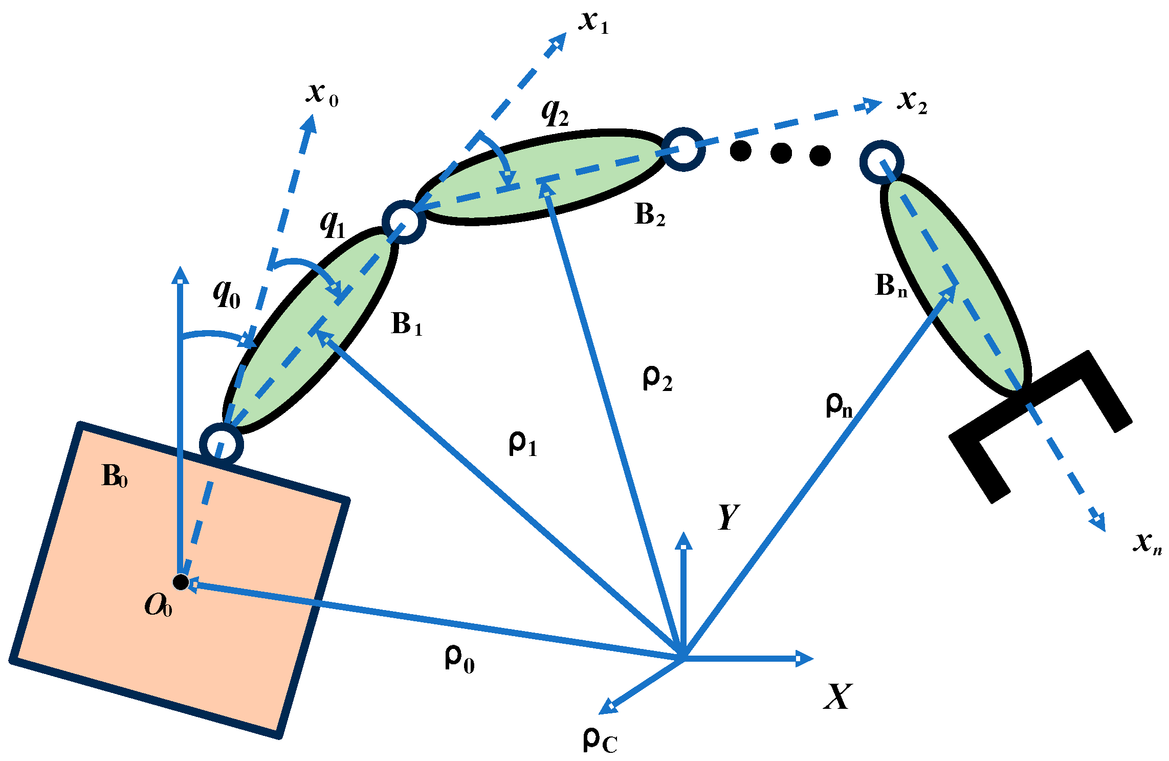
4. Numerical Simulations

To verify the effectiveness of the designed control algorithm, a system simulation is conducted using the space manipulator model depicted in Figure 1. The following system inertia parameters are taken:

$$\begin{array}{l}{m}_0=40\hspace{0.33em}\mathrm{kg}, m_1=4\hspace{0.33em}\mathrm{kg}, m_2=3\hspace{0.33em}\mathrm{kg}; l_0=1\hspace{0.33em}\mathrm{m}, l_1=1\hspace{0.33em}\mathrm{m}, l_2=1\hspace{0.33em}\mathrm{m}; J_0=16.67\hspace{0.33em}\mathrm{k}\mathrm{g}\cdot {\mathrm{m}}^2,\\ J_1=1.5\hspace{0.33em}\mathrm{k}\mathrm{g}\cdot {\mathrm{m}}^2, J_2=1.5\hspace{0.33em}\mathrm{k}\mathrm{g}\cdot {\mathrm{m}}^2; d_0=0.5\hspace{0.33em}\mathrm{m}, d_1=0.5\hspace{0.33em}\mathrm{m}, d_2=0.5\hspace{0.33em}\mathrm{m};\end{array}$$

The proposed simulation parameters are given as follows:

$$b_{i+}=5, b_{i-}=-5; h_{ri}=h_{li}=1; {\mathsf{{\rm Y}}}_{l1}{=\mathsf{{\rm Y}}}_{l2}{=\mathsf{{\rm Y}}}_{l3}=0.1+0.025\sin (t);$$

$${\mathsf{{\rm Y}}}_{u1}{=\mathsf{{\rm Y}}}_{u2}{=\mathsf{{\rm Y}}}_{u3}=0.1+0.02\sin (t); T_s=15; \sigma =0.5; \mathit{\Gamma }=diag[\begin{array}{ccc}1& 1& 1\end{array}];$$

The virtual control rate and the control gain of the controller are:

$${\mathit{K}}_1=diag\hspace{0.17em}[\begin{array}{ccc}2.5& 2.5& 2.5\end{array}]; {\mathit{K}}_2=diag\hspace{0.17em}[\begin{array}{ccc}0.1& 0.1& 0.1\end{array}];$$

$${\mathit{K}}_3=diag\hspace{0.17em}[\begin{array}{ccc}0.5& 1& 0.5\end{array}]; {\mathit{K}}_4=diag\hspace{0.17em}[\begin{array}{ccc}6& 2& 2\end{array}];$$

The parameters of the RBFNN are taken as follows: the number of base functions $i=5$, the parameter ${\sigma }_i$ of the center position of the basis function is taken according to the input range of the neural network, and its width $b$ is set to 5.

The initial state of the system is as follows: $q_0=1.5\hspace{0.17em}\hspace{0.17em}\mathrm{rad}$, $q_1=-1\hspace{0.17em}\mathrm{rad}$, and $q_2=-1\hspace{0.17em}\mathrm{rad}$; the second initial value is the following: $q_0=-1.2\hspace{0.17em}\hspace{0.17em}\mathrm{rad}$, $q_1=-0.8\hspace{0.17em}\hspace{0.17em}\mathrm{rad}$, and $q_2=-0.8\hspace{0.17em}\hspace{0.17em}\mathrm{rad}$; the third initial value is the following: $q_0=1\hspace{0.17em}\hspace{0.17em}\mathrm{rad}$, $q_1=-0.5\hspace{0.17em}\hspace{0.17em}\mathrm{rad}$, and $q_2=-0.5\hspace{0.17em}\hspace{0.17em}\mathrm{rad}$. The desired trajectory of the configuration is the following: $q_{d0}=\sin (t)$, $q_{d1}=\sin (t)$, and $q_{d2}=\sin (t)$. The simulation time is taken as 30 s.

4.1. Example 1

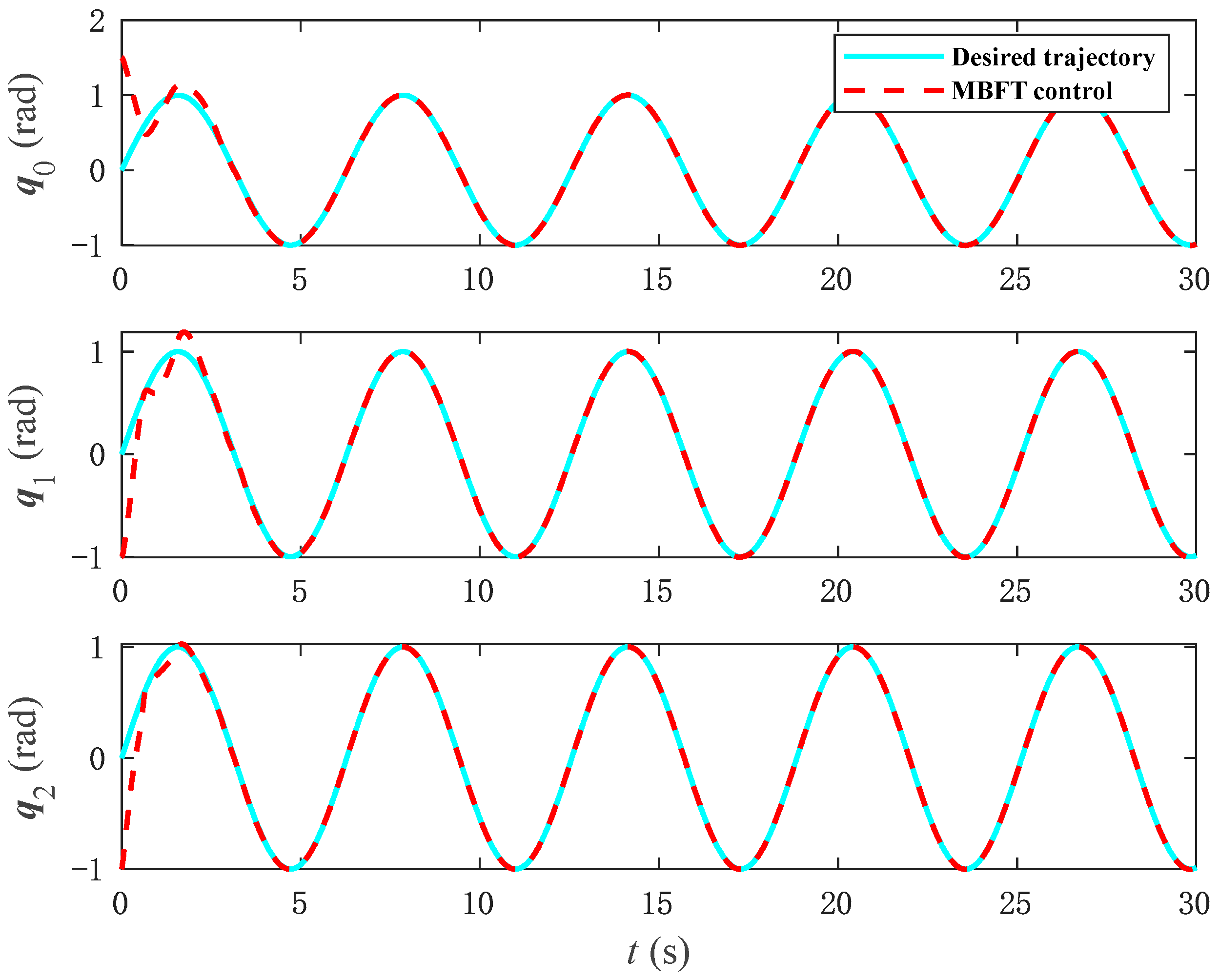
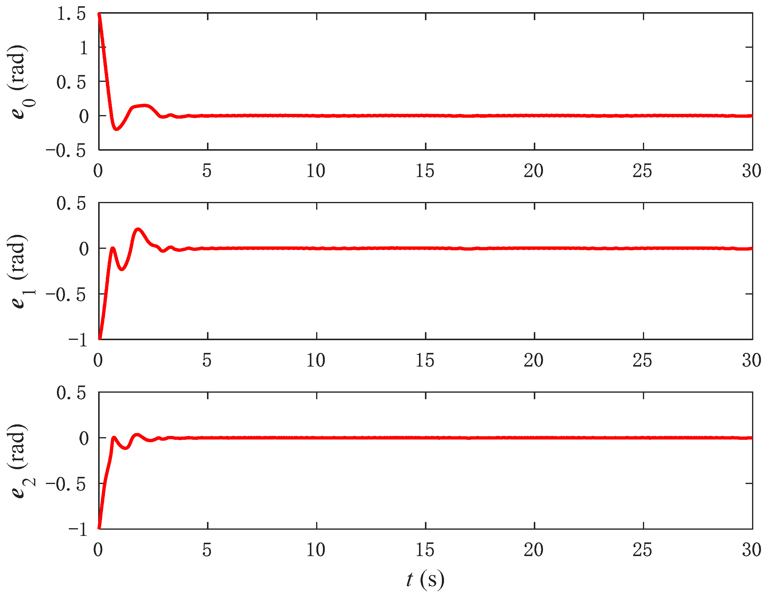
The simulation results of tracking performance based on model control are shown in Figure 5 and Figure 6. As illustrated in Figure 5, the model-based control method achieves rapid convergence within a fixed time period and demonstrates excellent tracking performance. Figure 6 illustrates the error conditions corresponding to the three joint angles. Based on the simulation results, it can be observed that, although the tracking errors of the three joint angles are small and eventually converge to a subset near zero, noticeable fluctuations still occur, particularly with significant error variation within the 0–3 s interval. From Figure 5 and Figure 6, it can be inferred that system uncertainty significantly impacts model-based control methods.

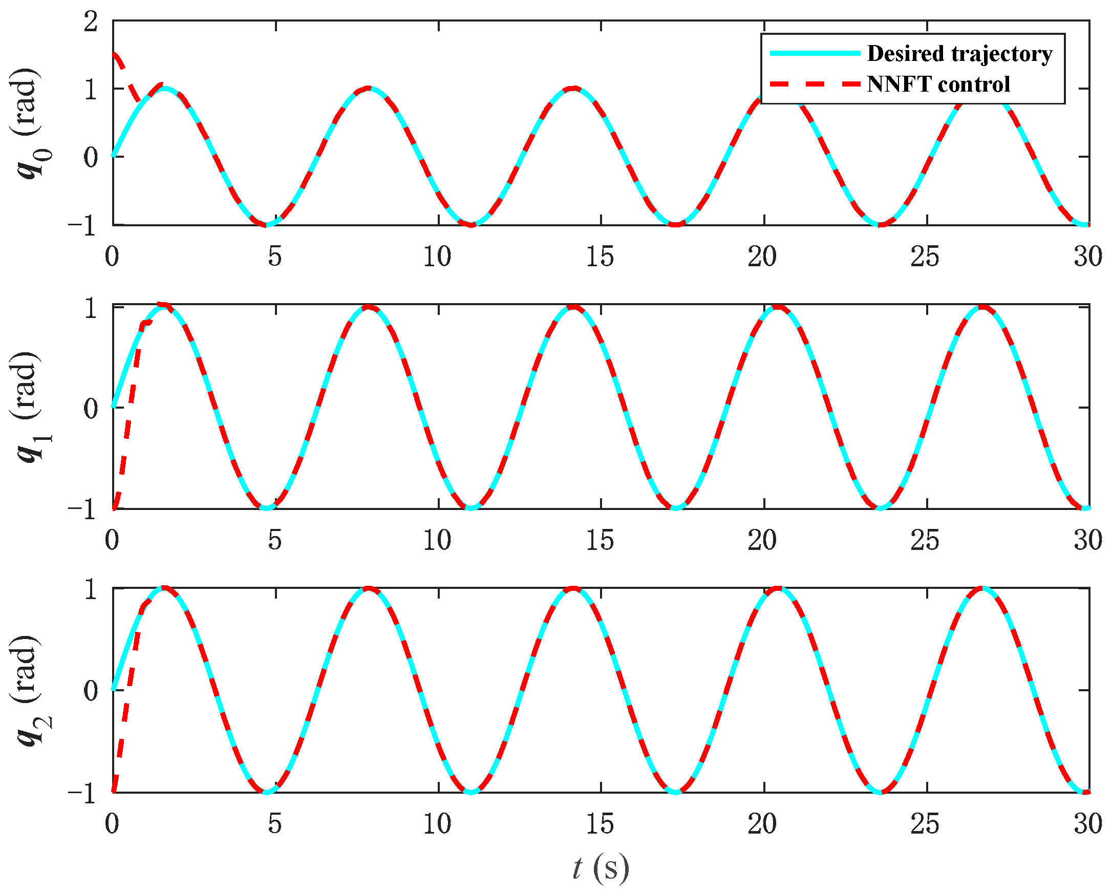
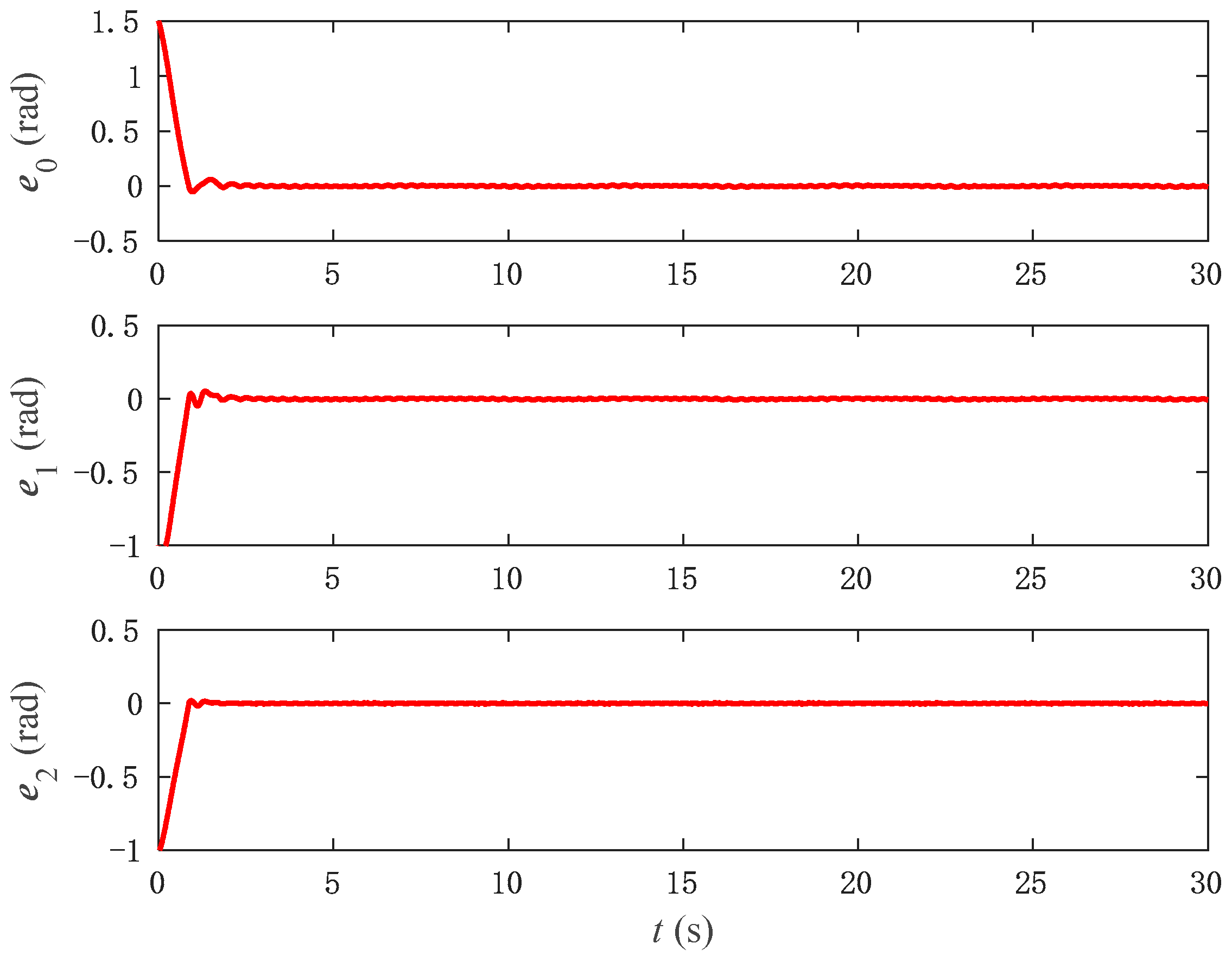
Between the existence of an input dead zone and the uncertainties inherent in the system, the MBFT control method exhibits limitations in accuracy. Consequently, NNFT is incorporated to enhance the control approach. The MBFT is also a type of adaptive sliding mode control. Figure 7, Figure 8 and Figure 9 depict the simulation outcomes of tracking performance under NNFT control. 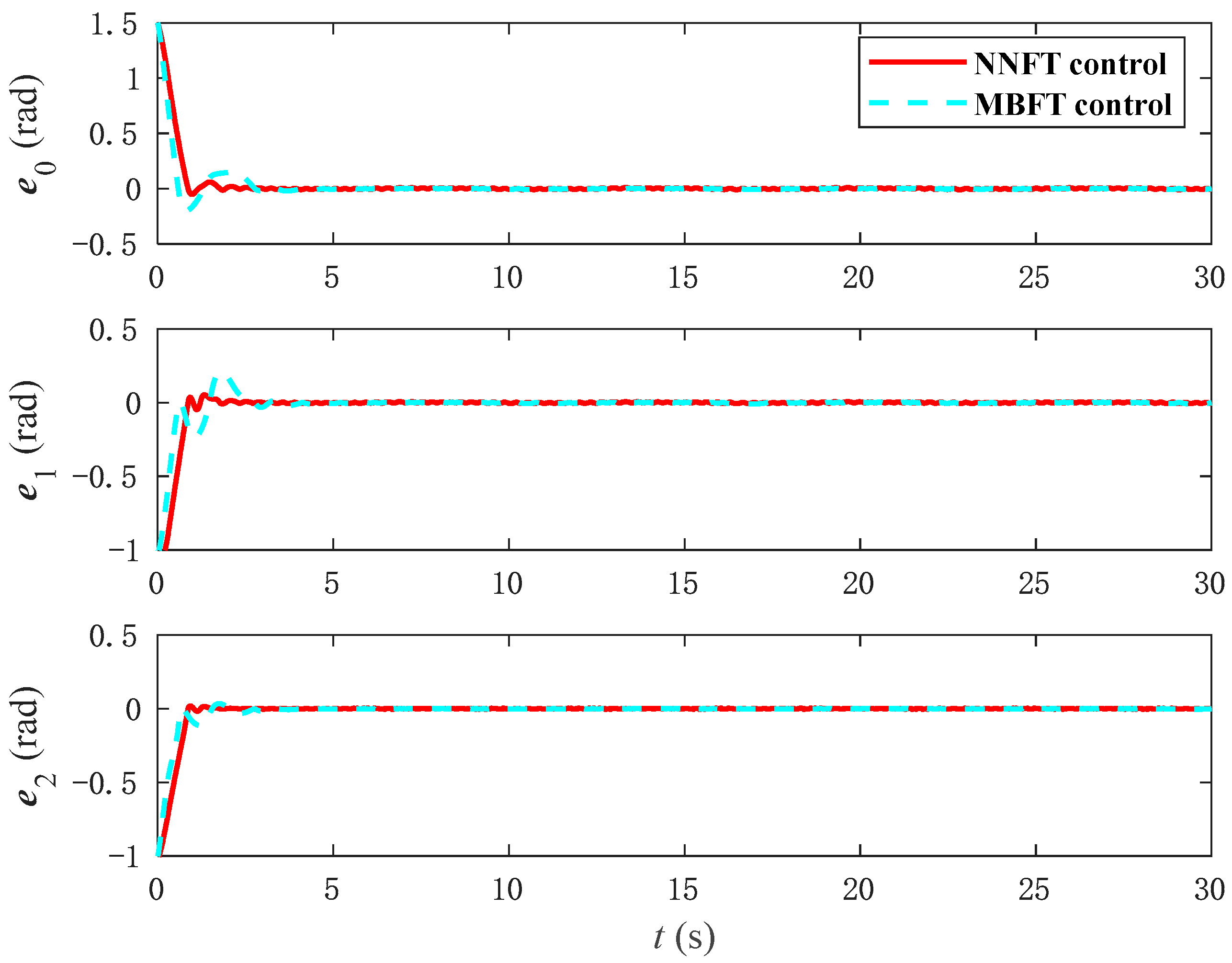Specifically, Figure 7 reveals that under neural network control, each joint angle of the space manipulator successfully attains the intended outcomes, as evidenced by Figure 8. It is evident that the tracking error of NNFT control is smaller than that of the previous model-based control, with a faster convergence speed that rapidly converges to zero and exhibits minimal fluctuations. For a clearer visual comparison, Figure 9 provides a comparison of the control errors between NNFT and MBFT. This underscores the superior performance of the NNFT control method compared to adaptive sliding mode control, where the neural network effectively compensates for the input dead zone and system uncertainties, resulting in stable tracking and improved accuracy.

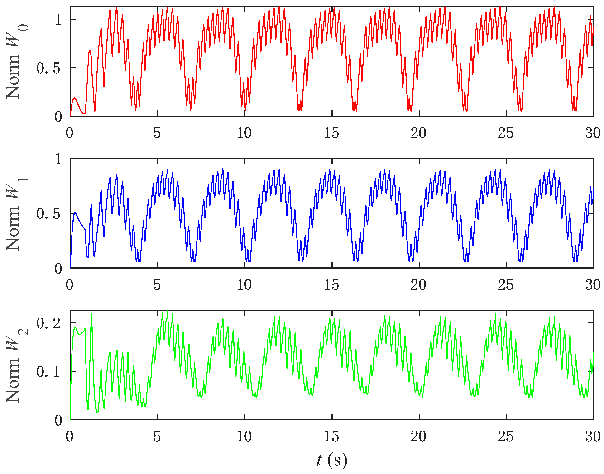
To further illustrate the effectiveness of the neural network, the updating of the weights of the neural network is analyzed. Figure 10 shows the process of updating the weights of the neural network. As can be observed, the neural network’s weights converge over time within a bound, demonstrating the ability of the neural network to compensate for the input dead zone and approximate the unknown dynamics of the system.

4.2. Example 2

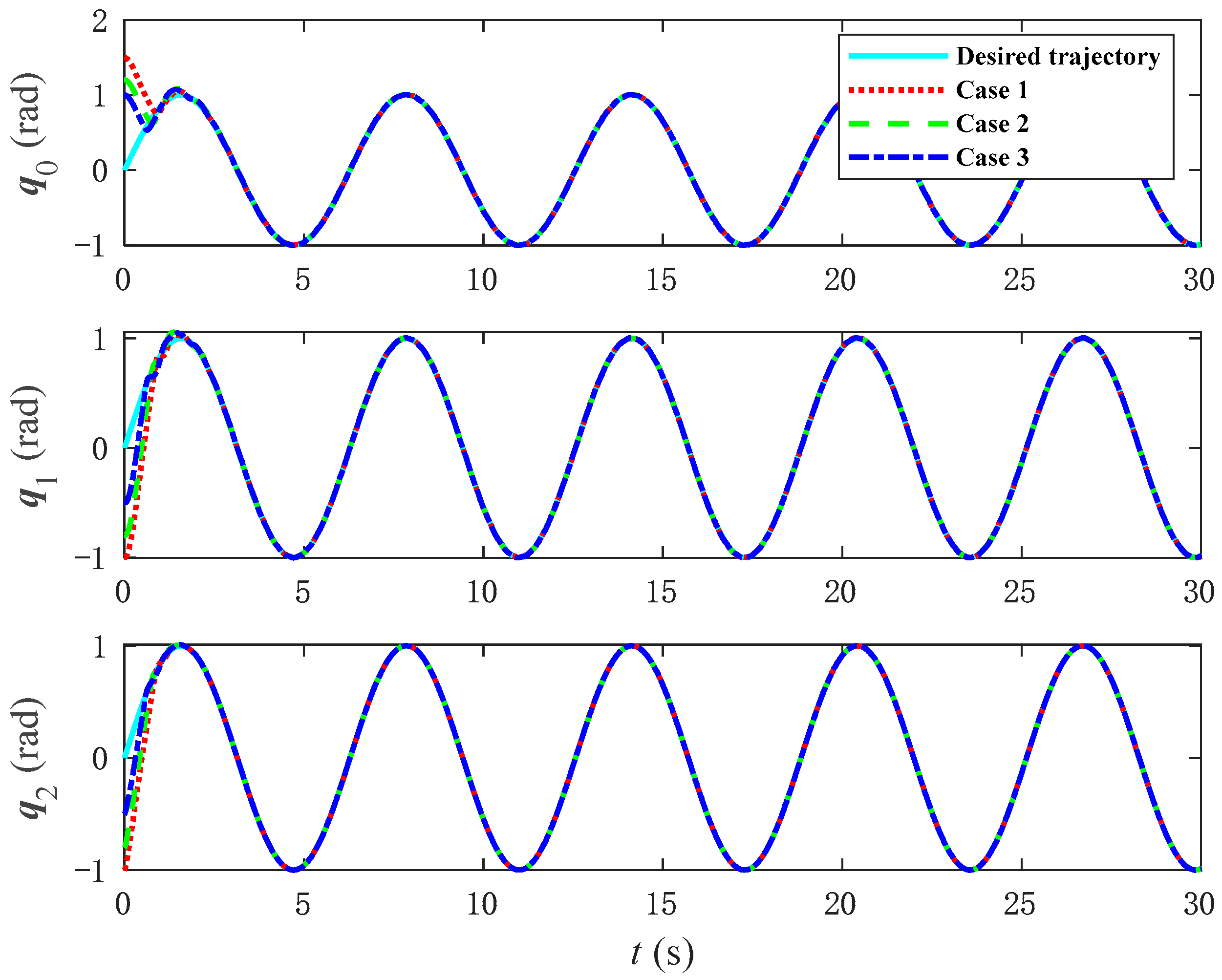
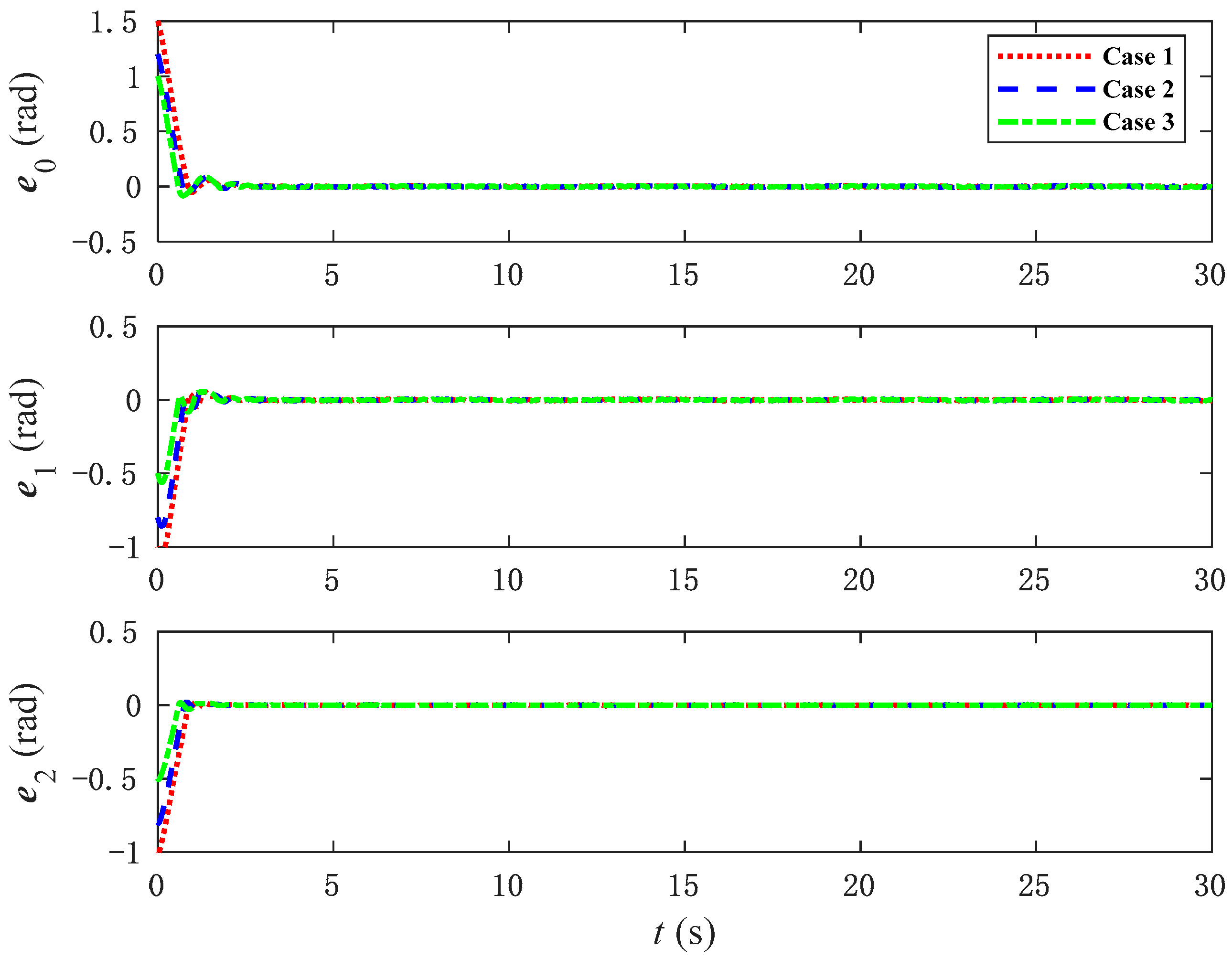
To verify the tracking performance of the NNFT control method, the initial values of the joint angles of the space manipulator are adjusted, and the tracking trajectories of the joint angles under different initial values are observed through simulation. Figure 11 shows the tracking trajectories of Case 1 ($q_0=1.5\hspace{0.17em}\mathrm{rad}$, $q_1=-1\hspace{0.17em}\mathrm{rad}$, $q_2=-1\hspace{0.17em}\mathrm{rad}$), Case 2 ($q_0=1.2\hspace{0.17em}\mathrm{rad}$, $q_1=-0.8\hspace{0.17em}\mathrm{rad}$, $q_2=-0.8\hspace{0.17em}\mathrm{rad}$), and Case 3 ($q_0=1\hspace{0.17em}\mathrm{rad}$, $q_1=-0.5\hspace{0.17em}\mathrm{rad}$,$q_2=-0.5\hspace{0.17em}\mathrm{rad}$) of the joint angles, respectively, and Figure 12 shows the corresponding tracking errors. It can be observed that, even with changes in the initial joint angle values, the proposed NNFT control method can still quickly track the trajectory with good control performance and fast convergence speed, while maintaining a small error. It compensates for both the joint dead zone and system uncertainties. Regardless of variations in the initial joint angles, as long as they are within a reasonable range and do not reach the maximum singular value of the joint angle, the proposed control method based on neural networks remains fully effective.

4.3. Example 3

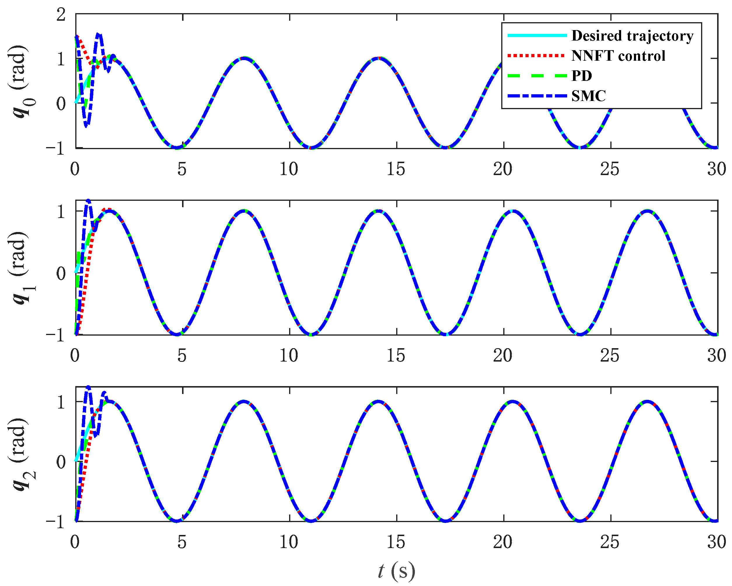
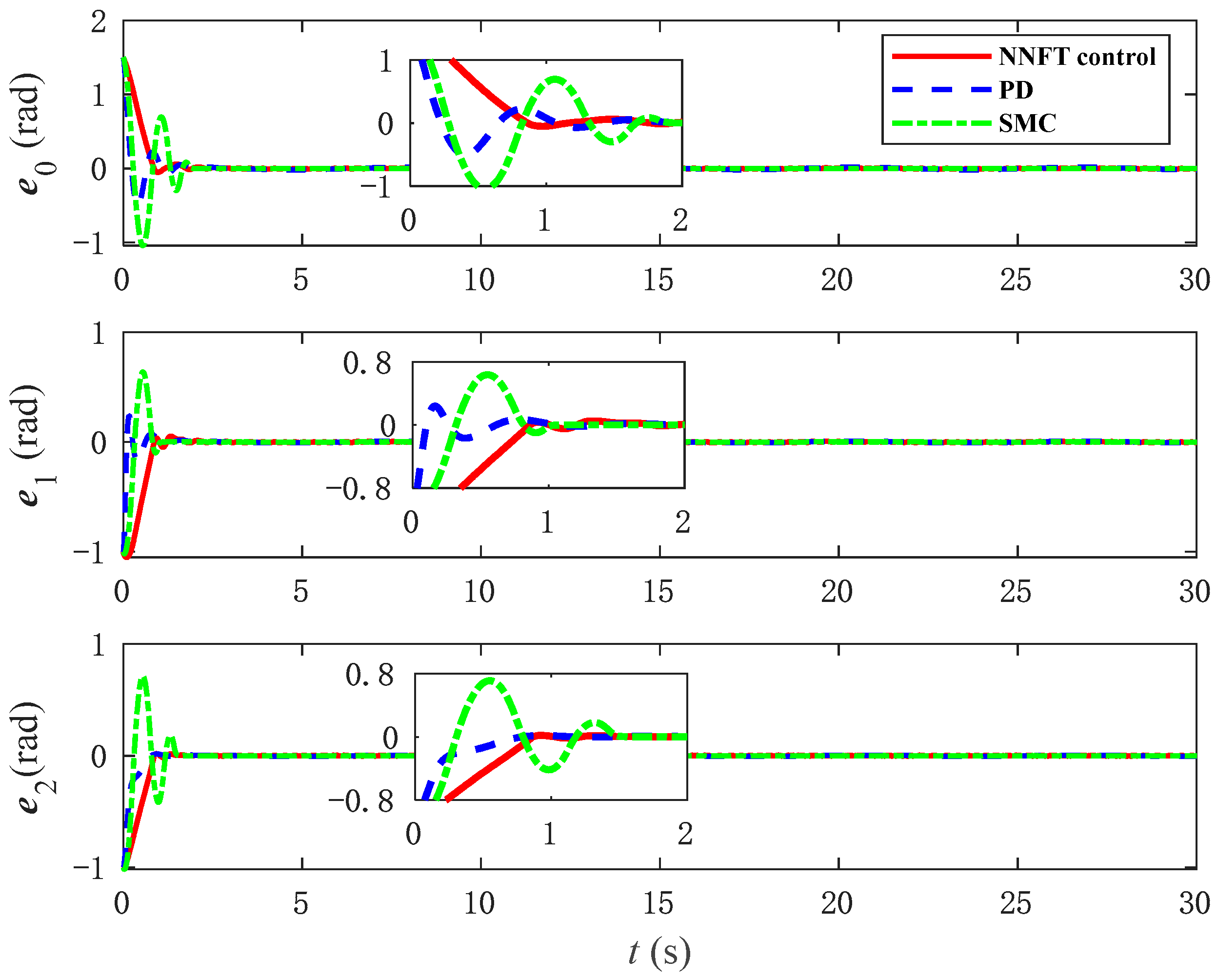
It is well known that traditional PD control offers high stability and is easy to implement, while sliding mode control has advantages such as higher precision, stronger robustness, better adaptability, and faster response speed. Therefore, the NNFT control method proposed in this paper is compared with these methods to verify the advantages of the proposed control approach. Figure 13 presents a comparative plot of joint angle trajectory tracking under three control methods, while Figure 14 displays the corresponding tracking error graphs. As evidenced by the two diagrams, the NNFT control method proposed in this paper enables a smoother approach to zero in terms of posture. 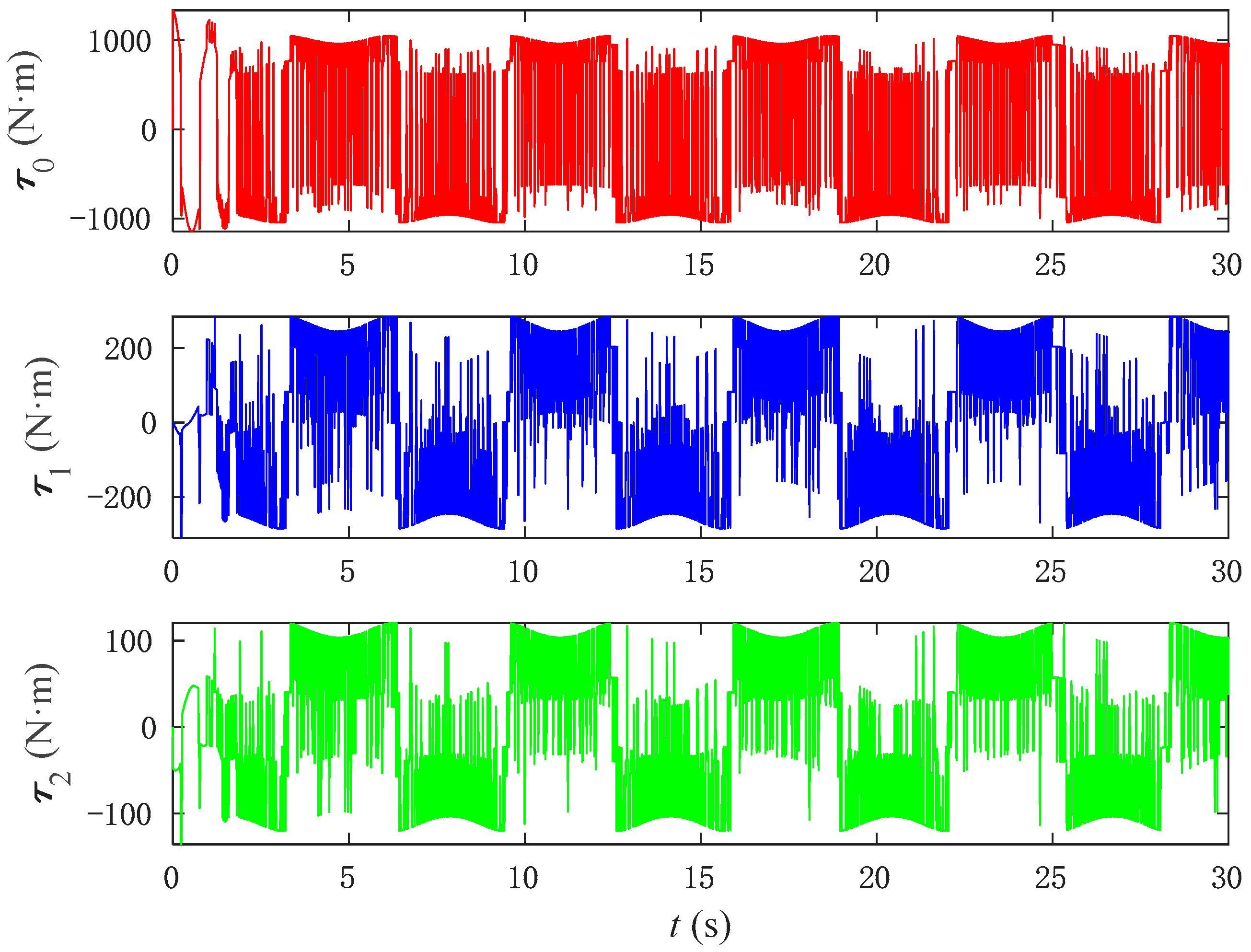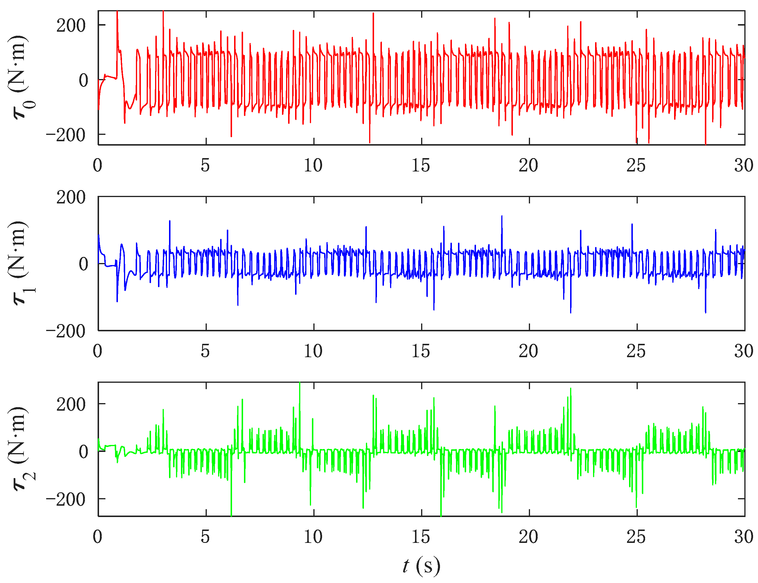In addition, as indicated in Figure 15, although the input torque of the PD control is relatively stable, it is excessively large, and such a large torque cannot be output in practical operating conditions. 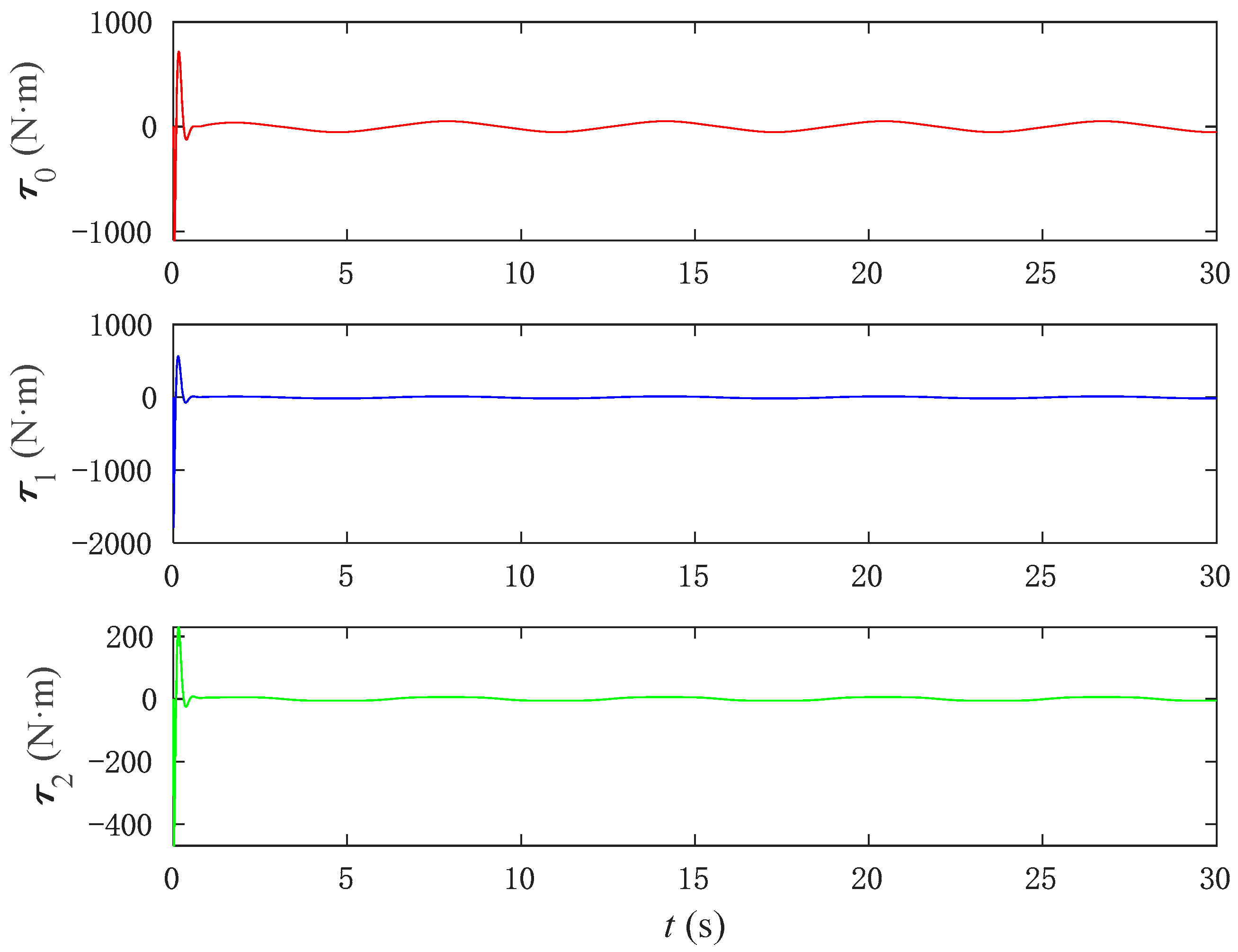In Figure 16, the input torque applied by the SMC to control the base joint angles is not only excessively large but also unstable across the joint angles. Compared to the NNFT control method shown in Figure 17, the output torque generated is smaller, remaining within an appropriate range, and exhibits stable performance. 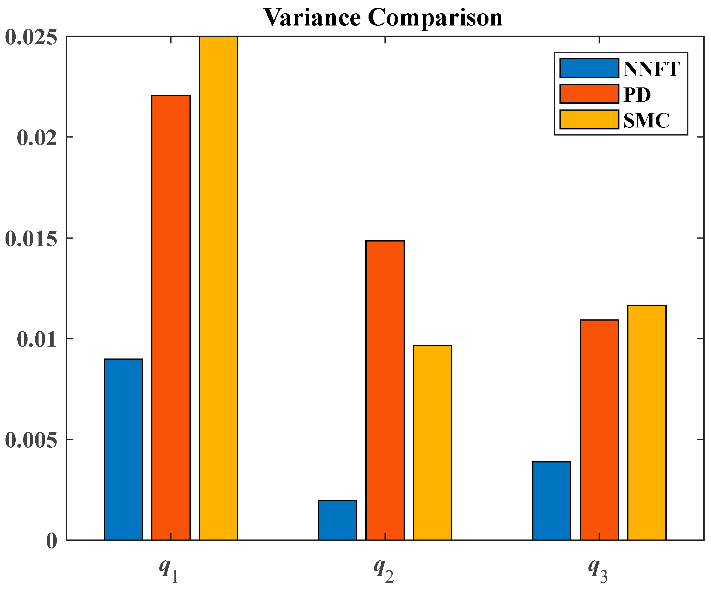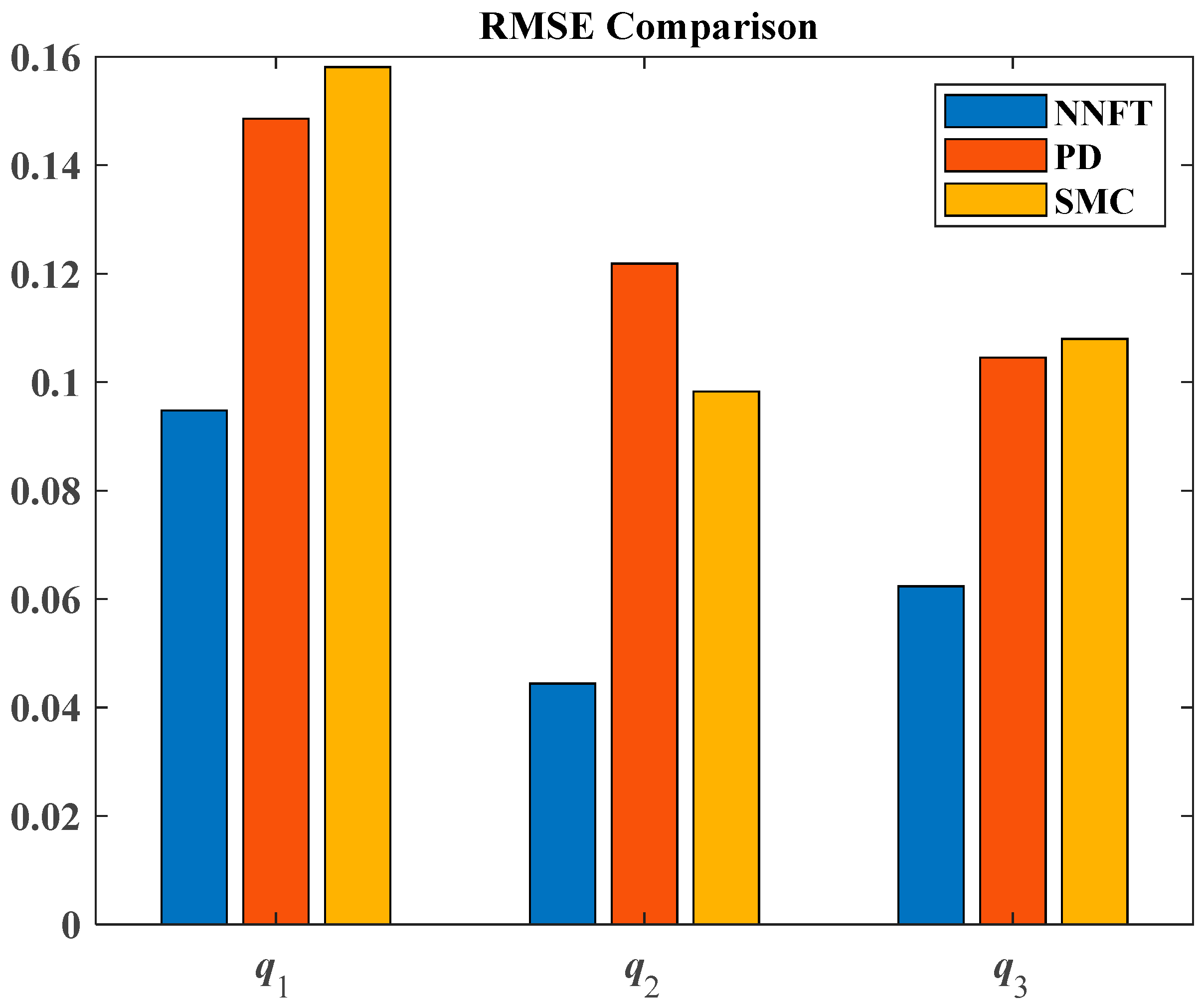Figure 18 and Figure 19 show the variances and root mean square errors of the three control methods, respectively. The bar charts indicate that the proposed control method has smaller error values, and has advantages. Based on the comparative analysis, the advantages of the fixed-time control method based on neural networks proposed in this paper are evident, demonstrating practical significance.

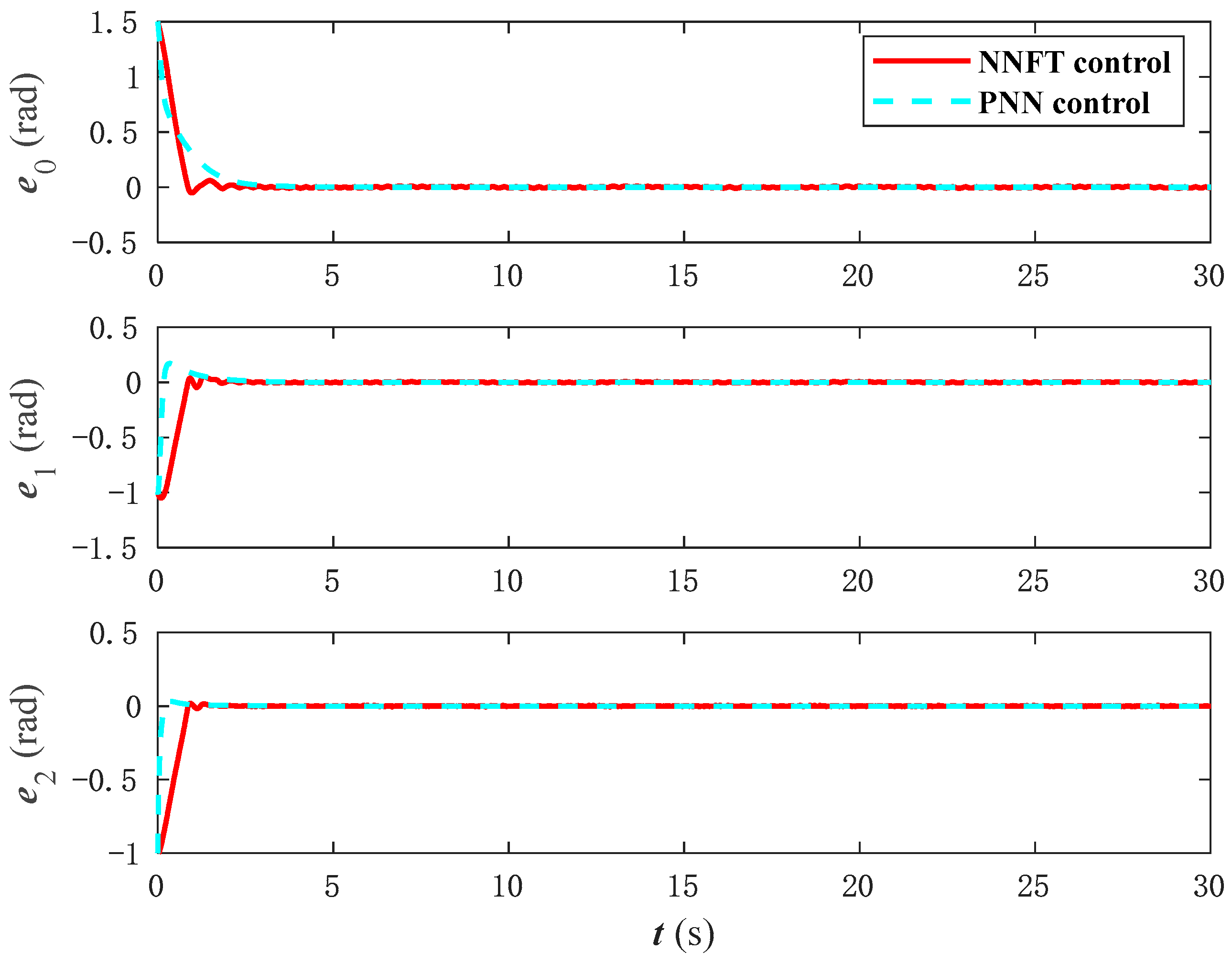
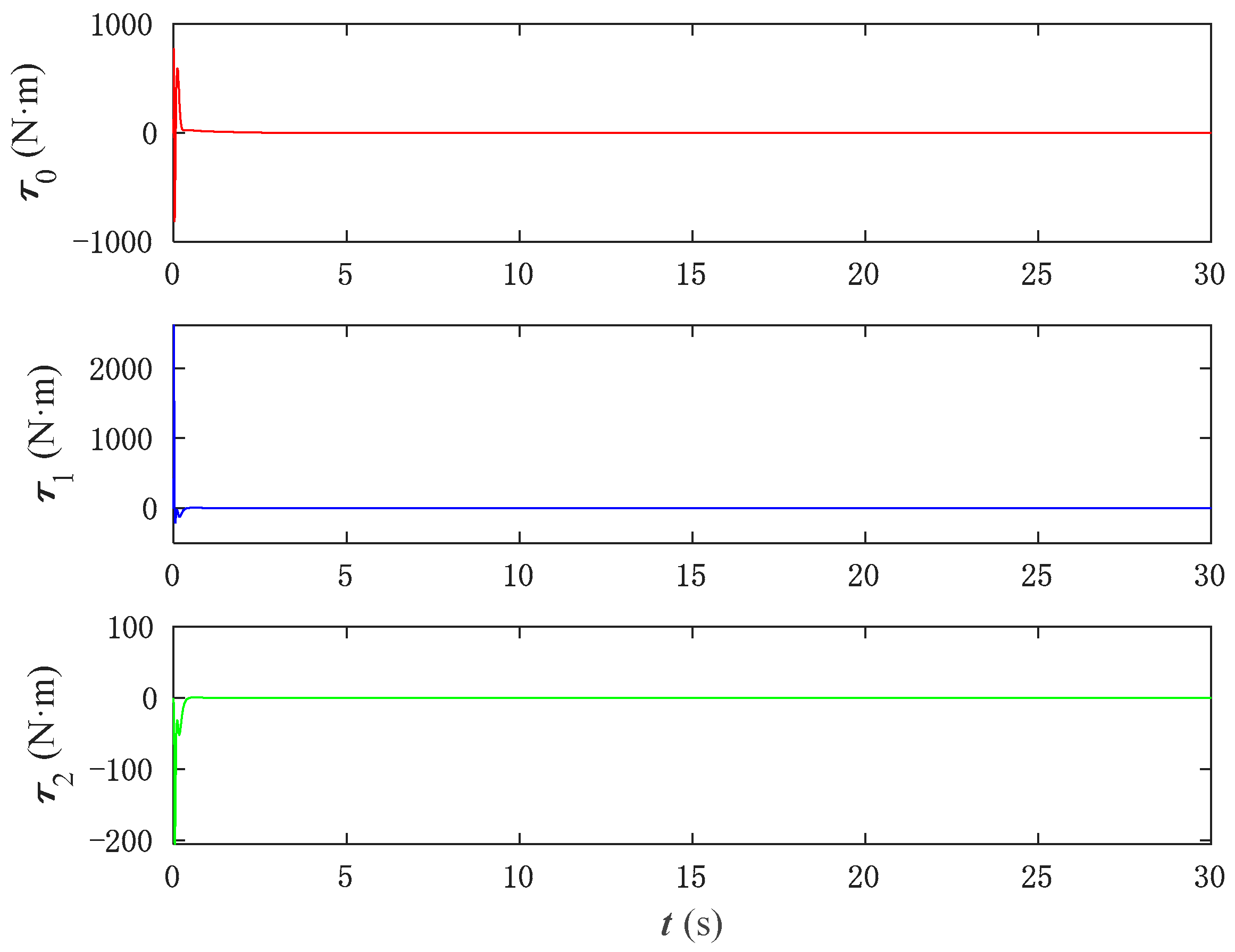
4.4. Example 4

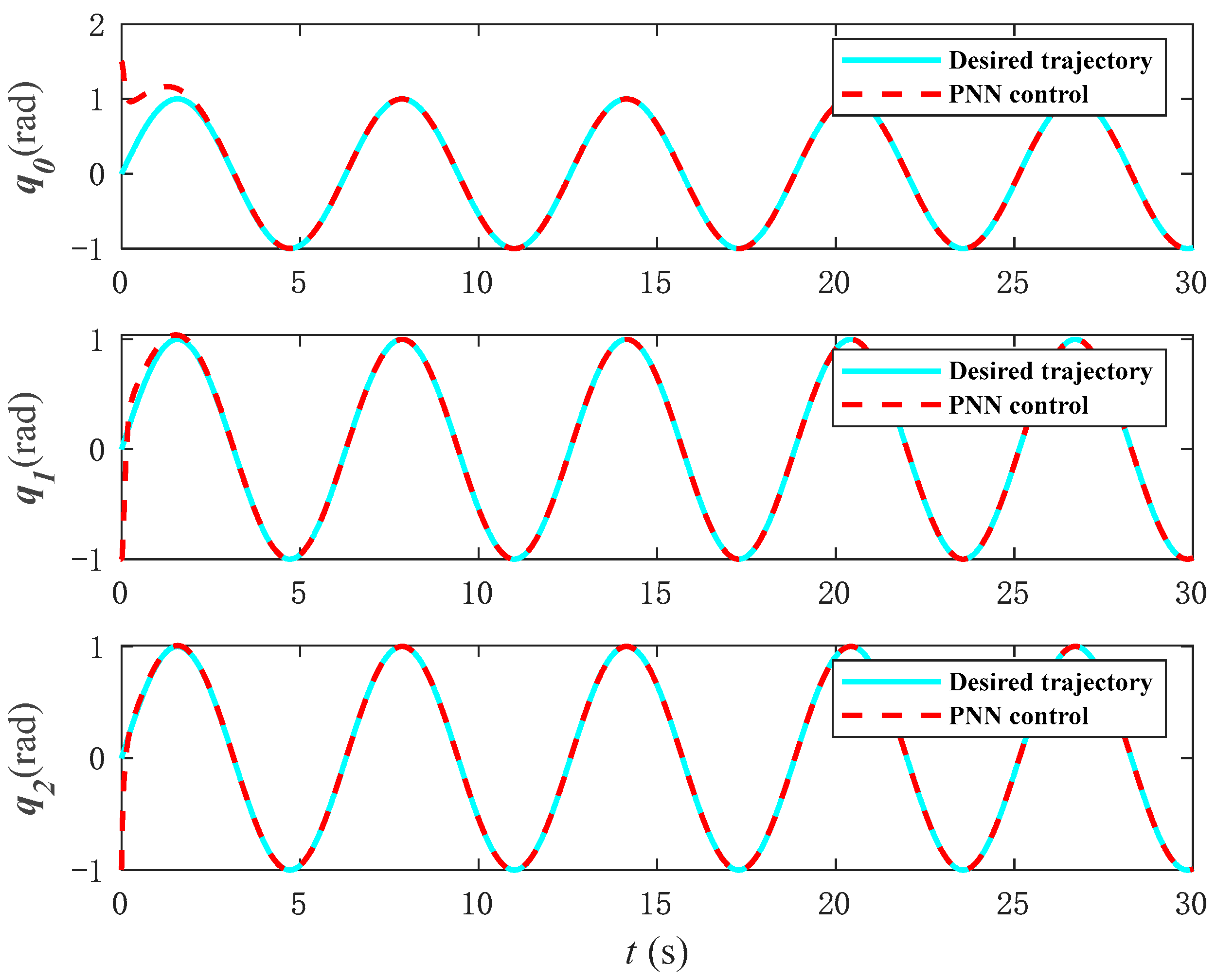
In order to highlight the superiority of the neural network and its update rate proposed in this paper, we compared it with the neural network proposed in Reference [46]. In Reference [46], the passivity-based neural network (PNN) control used is mainly used to compensate for disturbance terms in the slow variable subsystem of a flexible space manipulator. We apply its network structure and update rate to the system in this paper. Figure 20 shows the control performance of PNN control, and Figure 21 shows the error comparison between two control methods. It can be seen that the neural network control method proposed in this paper can converge and maintain stability in a faster time. However, from the torque input in Figure 22, it can be seen that the PNN control will exceed the limit of the actuator when the torque is too large in the initial stage of system control, which is not advisable. Therefore, the neural network and its update rate of the control algorithm proposed in this paper have better control performance.

5. Conclusions

In this paper, an adaptive neural network-based fixed-time control method is proposed to address the trajectory control problem of a space robot with uncontrollable position and attitude in the presence of an input dead zone. Within the framework of fixed-time convergence, a model-based control method is proposed. To address the adverse effects of uncertain system inertia parameters, an adaptive learning control method based on neural networks is further introduced. In order to enhance the learning rate of neural networks and achieve convergence of neural network weights within a fixed-time frame, a novel update rate method for neural networks is proposed. Additionally, addressing the issue of the joint input dead zone affecting the precision and stability of the space robot, a new adaptive law has been designed by integrating system error feedback and neural networks into the controller to compensate for these effects. Based on the Lyapunov stability theory, the stability of the closed-loop system is proven, and the trajectory tracking error is shown to converge to a small region around zero. Finally, the effectiveness of the control algorithm was validated through numerical simulation results. The presence of the input dead zone and associated uncertainties in a space robot is quite common in practical scenarios, underscoring the significance of studying such issues. In the future, new neural networks could be explored to address system uncertainties, and dead zone issues might be resolved using commentators, paving the way for more in-depth investigations into the control and trajectory tracking of space robots.

References

1. Cocuzza, S.; Pretto, I.; Debei, S. Least-Squares-Based Reaction Control of Space Manipulators. J. Guid. Control Dyn. 2012, 35, 976–986. [Google Scholar] [CrossRef]
2. Sandberg, A.; Sands, T. Autonomous Trajectory Generation Algorithms for Spacecraft Slew Maneuvers. Aerospace 2022, 9, 135. [Google Scholar] [CrossRef]
3. Yao, Q.; Li, Q.; Huang, M.; Jahanshahi, H. Predefined-time trajectory tracking control of free-flying space manipulator subject to uncertainties and disturbances. Robot. Auton. Syst. 2024, 177, 104699. [Google Scholar] [CrossRef]
4. Fu, X.; Ai, H.; Chen, L. Integrated sliding mode control with input restriction, output feedback and repetitive learning for space robot with flexible-base. Robotica 2023, 41, 370–391. [Google Scholar] [CrossRef]
5. Christidi-Loumpasefski, O.-O.; Papadopoulos, E. On the parameter identification of free-flying space manipulator systems. Robot. Auton. Syst. 2023, 160, 104310. [Google Scholar] [CrossRef]
6. Zhu, A.; Ai, H.; Chen, L. FSTSMC Compliance Control for Dual-Arm Space Robot with SDBD Capture Satellite Operation. J. Comput. Nonlinear Dyn. 2023, 18, 061006. [Google Scholar] [CrossRef]
7. Hu, Z.; Yuan, H.; Xu, W.; Yang, T.; Liang, B. Equivalent kinematics and pose-configuration planning of segmented hyper-redundant space manipulators. Acta Astronaut. 2021, 185, 102–116. [Google Scholar] [CrossRef]
8. Xu, R.; Luo, J.; Wang, M. Kinematic and dynamic manipulability analysis for free-floating space robots with closed chain con-straints. Robot. Auton. Syst. 2020, 130, 103548. [Google Scholar] [CrossRef]
9. Meng, Q.; Han, D.; Wang, Z. A model-free method for attitude estimation and inertial parameter identification of a noncoop-erative target. Adv. Space Res. 2023, 71, 1735–1751. [Google Scholar] [CrossRef]
10. Cao, Y.; Zhang, X.; Hao, Y.; Ge, X.; Cao, D. Coupled vibration analysis of the spacecraft with the flexible shaft and solar panels assembly. Aerosp. Sci. Technol. 2024, 151, 109259. [Google Scholar] [CrossRef]
11. Lu, H.; Wang, C.; Sun, C.; Li, A.; Zabolotnov, Y.M. Saturated Control of Space Tether System for Maneuvering Between Arbitrary Spinning Orientations. J. Guid. Control Dyn. 2024, 47, 2173–2181. [Google Scholar] [CrossRef]
12. Ullah, S.; Alsafran, A.S.; Harrison, A. A Uniform Robust Exact Differentiator Based Neuro-Fuzzy Fractional Order Sliding Mode Control for Optimal Standalone Solar Photovoltaic System. IEEE Access 2025, 13, 4411–4423. [Google Scholar] [CrossRef]
13. Ullah, S.; Khan, Q. Neuro-adaptive non-singular terminal sliding mode control for distributed fixed-time synchronization of higher-order uncertain multi-agent nonlinear systems. Inf. Sci. 2024, 659, 120087. [Google Scholar] [CrossRef]
14. Ullah, S.; Alghamdi, H.; Algethami, A.A. Robust Control Design of Under-Actuated Nonlinear Systems: Quadcopter Unmanned Aerial Vehicles with Integral Backstepping Integral Terminal Fractional-Order Sliding Mode. Fractal Fract. 2024, 8, 412. [Google Scholar] [CrossRef]
15. Chen, C.; Li, L.X.; Peng, H.P.; Yang, Y.X.; Mi, L.; Zhao, H. A new fixed-time stability theorem and its application to the fixed-time synchronization of neural networks. Neural Netw. 2020, 123, 412–419. [Google Scholar] [CrossRef] [PubMed]
16. Ding, Y.; Yue, X.; Liu, C.; Dai, H.; Chen, G. Finite-time controller design with adaptive fixed-time anti-saturation compensator for hypersonic vehicle. ISA Trans. 2022, 122, 96–113. [Google Scholar] [CrossRef]
17. Hu, J.; Zhang, X.; Zhang, D.; Chen, Y.; Ni, H.; Liang, H. Finite-time adaptive super-twisting sliding mode control for autonomous robotic manipulators with actuator faults. ISA Trans. 2024, 144, 342–351. [Google Scholar] [CrossRef]
18. Esmaeilzadeh, S.M.; Zeyghami, M.S. Nonlinear finite time attitude control of flexible spacecraft based on a novel output redefinition method. Chin. J. Aeronaut. 2023, 36, 373–385. [Google Scholar] [CrossRef]
19. Scalvini, A.; Suarez, A.; Nekoo, S.R.; Ollero, A. Finite-time state-dependent Riccati equation regulation of anthropomorphic dual-arm space manipulator system in free-flying conditions. Acta Astronaut. 2024, 216, 504–517. [Google Scholar] [CrossRef]
20. Sai, H.; Xu, Z.; He, S.; Zhang, E.; Zhu, L. Adaptive nonsingular fixed-time sliding mode control for uncertain robotic manipulators under actuator saturation. ISA Trans. 2022, 123, 46–60. [Google Scholar] [CrossRef]
21. Van, M.; Ceglarek, D. Robust fault tolerant control of robot manipulators with global fixed-time convergence. J. Frankl. Inst. 2021, 358, 699–722. [Google Scholar] [CrossRef]
22. Jin, R.; Rocco, P.; Geng, Y. Observer-based fixed-time tracking control for space robots in task space. Acta Astronaut. 2021, 184, 35–45. [Google Scholar] [CrossRef]
23. Zhang, H.; Zheng, Y.; Wang, Y. Event-triggered fault-tolerant attitude tracking control for spacecraft with fixed-time controller and disturbance observer under input constraints. Adv. Space Res. 2024, 73, 3148–3165. [Google Scholar] [CrossRef]
24. Shen, G.; Huang, P.; Zhang, F.; Ma, Z.; Xia, Y. Adaptive Fixed-Time Control for the Postcapture Tethered Spacecraft With Full-State Constraints. IEEE Trans. Aerosp. Electron. Syst. 2023, 59, 2702–2712. [Google Scholar] [CrossRef]
25. Ferede, R.; Croon, G.; Wagter, C.D.; Izzo, D. End-to-end neural network based optimal quadcopter control. Robot. Auton. Syst. 2024, 172, 0921–8890. [Google Scholar] [CrossRef]
26. Yang, Z.; Peng, J.; Liu, Y. Adaptive neural network force tracking impedance control for uncertain robotic manipulator based on nonlinear velocity observer. Neurocomputing 2019, 331, 263–280. [Google Scholar] [CrossRef]
27. Boukens, M.; Boukabou, A.; Chadli, M. Robust adaptive neural network-based trajectory tracking control approach for non-holonomic electrically driven mobile robots. Robot. Auton. Syst. 2017, 92, 30–40. [Google Scholar] [CrossRef]
28. Zhang, W.; Shen, J.; Ye, X.; Zhou, S. Error model-oriented vibration suppression control of free-floating space robot with flexible joints based on adaptive neural network. Eng. Appl. Artif. Intell. 2022, 114, 105028. [Google Scholar] [CrossRef]
29. Yu, L.; Qiu, Z.; Zhang, X. Radial basis function neural network vibration control of a flexible planar parallel manipulator based on acceleration feedback. J. Vib. Control 2022, 28, 351–363. [Google Scholar] [CrossRef]
30. Liu, H.; Li, X.; Dong, M. Robotic Motion Planning Based on Deep Reinforcement Learning and Artificial Neural Networks. IEEE Trans. Autom. Sci. Eng. 2025, 22, 8465–8479. [Google Scholar] [CrossRef]
31. Zhang, Y.; Xu, Z.; Chen, J. Neural networks-based composite learning control for robotic systems with predefined time error constraints. Neurocomputing 2024, 608, 128414. [Google Scholar] [CrossRef]
32. Liu, L.; Lu, Y.; Gu, X. Post-capture tracking control with fixed-time convergence for a free-flying flexible-joint space robot based on adaptive neural network. Neural Comput. Appl. 2024, 36, 4661–4667. [Google Scholar] [CrossRef]
33. Jia, X.; Xu, S.; Qi, Z.; Zhang, Z.; Chu, Y. Adaptive output feedback tracking of nonlinear systems with uncertain nonsymmetric dead-zone input. ISA Trans. 2019, 95, 35–44. [Google Scholar] [CrossRef]
34. Wang, Y.; Tao, F.; Fu, Z.; Wang, N.; Chen, Q. Adaptive fuzzy fixed-time dynamic surface control for stochastic nonstrict nonlinear systems with unknown dead-zones. J. Frankl. Inst. 2023, 360, 4091–4113. [Google Scholar] [CrossRef]
35. Xia, Y.; Liu, Y.; Sun, W. Disturbance observer-based full-state constrained control for robotic systems with dead zone. J. Frankl. Inst. 2022, 360, 14630–14644. [Google Scholar] [CrossRef]
36. Javaid, U.; Zhen, Z.; Shahid, S.; Ibrahim, D.S.; Ijaz, S. Observer-based attitude control of spacecraft under actuator dead zone and misalignment faults. Appl. Math. Comput. 2024, 465, 128406. [Google Scholar] [CrossRef]
37. Sankaranarayanan, V.; Banerjee, A.; Satpute, S.; Roy, S.; Nikolakopoulos, G. Adaptive control for a payload carrying spacecraft with state constraints. Control Eng. Pract. 2023, 135, 105515. [Google Scholar] [CrossRef]
38. Sankaranarayanan, V.; Satpute, S.; Roy, S.; Nikolakopoulos, G. Adaptive Control of Euler-Lagrange Systems under Time-varying State Constraints without a Priori Bounded Uncertainty. IFAC-PapersOnLine 2023, 56, 3360–3365. [Google Scholar] [CrossRef]
39. Ni, J.; Ahn, C.; Liu, L.; Liu, C. Prescribed performance fixed-time recurrent neural network control for uncertain nonlinear systems. Neurocomputing 2019, 363, 351–365. [Google Scholar] [CrossRef]
40. Wang, H.; Meng, Z. Fixed-time adaptive neural tracking control for high-order nonlinear switched systems with input saturation and dead-zone. Appl. Math. Comput. 2024, 480, 128904. [Google Scholar] [CrossRef]
41. Wu, Z.; Zou, Z.; Bu, X.; Zhang, J.; Ma, K. Fixed-time neural network composite learning control for uncertain nonlinear systems. Eng. Appl. Artif. Intell. 2025, 141, 109722. [Google Scholar] [CrossRef]
42. Zhu, Z.; Xia, Y.; Fu, M. Attitude stabilization of rigid spacecraft with finite-time convergence. Int. J. Robust Nonlinear Control 2015, 21, 686–702. [Google Scholar] [CrossRef]
43. Jin, X. Adaptive fixed-time control for MIMO nonlinear systems with asymmetric output constraints using universal barrier functions. IEEE Trans. Autom. Control 2019, 64, 3046–3053. [Google Scholar] [CrossRef]
44. Wang, H.; Bing, C.; Chong, L.; Bing, C.; Chong, L. Adaptive neural tracking control for a class of stochastic nonlinear systems. IEEE Trans. Neural Networks Learn. Syst. 2014, 25, 1262–1280. [Google Scholar] [CrossRef]
45. Zuo, Z.; Tian, B.; Defoort, M.; Ding, Z. Fixed-time consensus tracking for multiagent systems with high-order integrator dynamics. IEEE Trans. Autom. Control 2018, 63, 563–570. [Google Scholar] [CrossRef]
46. Ai, H.; Chen, L. Passivity-based neural network H∞ avoidance compliant control of space robot capturing spacecraft. Opt. Precis. Eng. 2020, 28, 717–726. [Google Scholar] [CrossRef]
Figure 1. Model of a space manipulator.
Aerospace 12 00593 g001
Figure 2. Model of input dead zone.
Aerospace 12 00593 g002
Figure 3. Model of RBFNN.
Aerospace 12 00593 g003
Figure 4. Diagram of the NNFT controller.
Aerospace 12 00593 g004
Figure 5. MBFT control tracking performances.
Aerospace 12 00593 g005
Figure 6. MBFT control tracking errors.
Aerospace 12 00593 g006
Figure 7. NNFT control tracking performances.
Aerospace 12 00593 g007
Figure 8. NNFT control tracking errors.
Aerospace 12 00593 g008
Figure 9. NNFT control and MBFT control errors.
Aerospace 12 00593 g009
Figure 10. Neural network weights for the NNFT control.
Aerospace 12 00593 g010
Figure 11. NNFT control tracking performances with different initial values.
Aerospace 12 00593 g011
Figure 12. NNFT control tracking errors with different initial values.
Aerospace 12 00593 g012
Figure 13. Tracking performance comparison of the NNFT control with PD and SMC.
Aerospace 12 00593 g013
Figure 14. Tracking error comparison of the NNFT control with PD and SMC.
Aerospace 12 00593 g014
Figure 15. Control input for the PD.
Aerospace 12 00593 g015
Figure 16. Control input for the SMC.
Aerospace 12 00593 g016
Figure 17. Control input for the NNFT control.
Aerospace 12 00593 g017
Figure 18. Variance comparison of NNFT, PD, and SMC.
Aerospace 12 00593 g018
Figure 19. RMSE comparison of NNFT, PD, and SMC.
Aerospace 12 00593 g019
Figure 20. PNN control tracking performances.
Aerospace 12 00593 g020
Figure 21. NNFT control and PNN control errors.
Aerospace 12 00593 g021
Figure 22. Control input for the PNN control.
Aerospace 12 00593 g022
Disclaimer/Publisher’s Note: The statements, opinions and data contained in all publications are solely those of the individual author(s) and contributor(s) and not of MDPI and/or the editor(s). MDPI and/or the editor(s) disclaim responsibility for any injury to people or property resulting from any ideas, methods, instructions or products referred to in the content.