Multi-Objective Optimization Method for Multi-Module Micro–Nano Satellite Components Assignment and Layout

Abstract

The assembly optimization design of satellite components is a crucial element in the overall design of satellites. In this paper, a novel three-dimensional assembly optimization design problem (3D-AODP) for multi-module micro–nano satellite components is proposed according to the engineering requirements, aiming at optimizing the satellite mass characteristics, and taking into account constraints such as space interference, space occupation and special location. Multi-module micro–nano satellites are a new type of satellite configuration based on the assembly of multiple U-shaped cube units. The 3D-AODP of its components is a challenging two-layer composite optimization task involving discrete variable optimization of component allocation and continuous variable optimization of component layout, which interact with each other. To solve the problem, a hybrid assembly optimization method based on tabu search (TS) and multi-objective differential evolutionary (MODE) algorithms is proposed, in which the assignment problem of the components is converted into a domain search problem by the TS algorithm. The space interference constraints and space occupancy constraints of the components are considered, and an assignment scheme with the minimum mass difference is obtained. On this basis, a bi-objective differential evolutionary algorithm is used to develop the layout optimization problem for the components, which takes into account the spatial non-interference constraints and special location constraints of the components, and obtains the Pareto solution set of the assembly scheme under the optimal mass characteristics (moment of inertia and product of inertia). Finally, the feasibility and effectiveness of the proposed method is demonstrated by an engineering case.

1. Introduction

In recent years, due to their advantages of small size, low cost and short cycle time, micro–nano satellites have been widely used in major universities and research institutions around the world, and have shown wide application prospects in the fields of scientific and technological validation, remote sensing and deep space exploration [1,2,3]. With the continuous expansion of satellite application scenarios and the upgrading of the complexity and diversity of missions, there is an increasingly urgent demand for effective and efficient satellite overall design methods [4,5,6]. The assembly optimization design of satellite components has become a key research area of satellite overall design, which aims to achieve better performance of satellites by reasonably planning the installation positions of components within the satellite. However, as the size of satellite configuration and the number of components increase, it brings great challenges to the optimal design of satellite assembly, especially for micro–nano satellites assembled by multiple modules; how to reasonably plan the integration position of components has become a key challenge [7,8,9].

The optimal design of satellite component assembly has a direct impact on its performance and lifetime, and most of the existing studies on satellite assembly optimization problems only focus on layout optimization problems, which is due to the fact that the assignment schemes of components and modules are determined in advance, which means that there is no need to consider to which module the component belongs to, and only the installation position of the component in the determined space needs to be taken into account. However, if the assignment scheme of the components itself is problematic, it will seriously restrict the further improvement of the optimized design level, and it is even impossible to find a feasible solution that meets the technical requirements [10]. Therefore, the optimization problem of component assignment for multi-module micro–nano satellites needs to be focused on. In fact, both the assignment problem and the layout problem of the components belong to the Non-deterministic Polynomial Hard (NP-Hard) problem, and the assembly optimization problem formed after the integration of the two is even more difficult to solve.

Early micro–nano satellites have simple functions and a small number of components, coupled with a very limited layout space; the satellite layout optimization problem is often solved by mathematical solutions combined with manual experience. However, these design methods are cumbersome and resource-consuming, and cannot fully utilize the potential of the design space, leading to a significant increase in the difficulty of satellite layout optimization design. To address these challenges, researchers have proposed a large number of novel mathematical methods and applied them to the solution of optimization problems, such as mathematical programming methods, graph theory and topology [11], which usually rely on accurate mathematical models. However, the optimization model in real engineering will be inevitably affected by a variety of uncertain conditions such as external interference and system coupling, while mathematical methods relying on accurate models have difficulty effectively and efficiently solving the assembly optimization design problems faced in real engineering. For this reason, researchers have begun to use mature computer technology to solve the satellite assembly optimization problem using intelligent algorithms, which are mainly based on heuristic algorithms, including genetic algorithms [12], ant colony algorithms [13], particle swarm algorithms [14], search algorithms [15], etc. These algorithms can avoid the excessive reliance on the precise optimization model, and make the layout optimization problem solution more efficient than ever before, which improves the efficiency unprecedentedly.

Grignon and Fadel [16] applied a genetic algorithm (GA) to the small satellite equipment layout optimization problem to obtain the optimal solution with the satellite’s compactness, load balance and maintainability as the optimization objectives. Teng [17] proposed a two-system cooperative co-evolutionary algorithm (known as Oboe-CCEA) to address the optimization problem of this system. Xu [18] proposed a genetic algorithm to accomplish the optimal layout of the components of the satellite section. Gamot [14] proposed a genetic algorithm based on the hidden variable mechanism to solve the design variable space problem of the spacecraft. Ye [19] gave a two-population genetic algorithm to improve and enhance the heat dissipation performance. ZHONG [10] obtained a better performance of the satellite by dynamically assigning components to the satellite in the optimization process. Xu [20] used a heuristic algorithm to accomplish the optimal assignment of components and solved the key indicators of the integrated satellite by an evolutionary algorithm. Chen [21] used an accelerated particle swarm optimization algorithm to search for the optimal layout scheme, which reduces the effect of residual magnetic field on the satellite’s attitude. Meller [22] introduced a simulated annealing algorithm to solve the problem of the facility layout. Liu [23] proposed a multi-objective particle swarm optimization algorithm to solve the layout problem of unequal area facilities. In order to explicitly express and deal with the constraints, Chen [24] proposed a phi function method for accurately describing the distances of components to prevent overlapping problems. With the birth of multi-module satellites, some researchers regarded the problem as a system optimization problem and used a system decomposition strategy to solve it. Cuco [25] designed a multi-objective optimization framework for the layout optimization problem and used a fast elite non-dominated sequential genetic algorithm (NSGA-II) to obtain its Pareto solution set. Fakoor [26], using the moment of inertia as the optimization objective, investigated the configuration design of a simplified communication satellite. In addition to non-interference and satellite stabilization, dispersion and aggregation of certain components were added as constraints. Fakoor [27] provided an optimization tool, Spacecraft Component Adaptive Layout Environment (SCALE), for the spacecraft component layout problem.

The component layout problem has been well studied in the above literature, but the component assignment problem has not been discussed. It is worth noting that although the satellites have multiple support surfaces, they have only one module in which the layout space for positioning the components is continuous. During the optimization process, components can move freely in this layout space. To ensure that all components are affixed to the support surfaces, they are affixed to the nearest support surface around them. In 2017, a layout design of a space station with six modules divided by three partitions was studied [13]. To deal with the component assignment problem, a tabu search for component assignments applied this method to a simplified satellite re-entry module layout design [25]. In addition to these algorithms, a grouped genetic algorithm with problem-oriented crossover and mutation for this problem was developed [15].

The above studies have conducted a lot of research on the assignment optimization and layout optimization of satellite components. However, most of the existing studies focus on segmented large satellites (e.g., communication satellites, return capsule satellites, etc.) or small satellites, and there are fewer studies on the assignment optimization and layout optimization of components for multi-module micro–nano satellites.

To solve this problem, this paper introduces the 3D component assignment and layout optimization (3D-RMSAO) problem for multi-module micro–nano satellites based on practical engineering requirements, which is used to optimize the mass difference and mass characteristics (moment of inertia (MOI) and product of inertial (POI)) of the satellites by strategically assigning the components to the appropriate modules and rationally planning the installation satellites for the components in the corresponding modules. It should be supplemented that this paper mainly takes the mechanical optimization of satellites as the design objective. Considering the functional requirements of components and the interrelationships between components, the constraints in 3D spatial layout optimization design are proposed and solved, including non-interference constraints, occupancy constraints and specific location constraints. These constraints play a key role in determining the precise location of components within modules. Additionally, while previous studies have primarily focused on component position optimization (continuous variable optimization), 3D-RMSAO also requires consideration of component assignment optimization (discrete variable optimization) at the same time.

In this paper, a hybrid algorithm based on tabu search (TS) and multi-objective differential evolution (MODE) is proposed to optimize the mass characteristics of a multi-module micro–nano satellite and to obtain the optimal layout scheme. The TS algorithm is used to achieve the optimal assignment of components and minimize the mass difference of the satellite, which is the basis for the layout optimization design. The TS algorithm is used to achieve the optimal assignment of components, which minimizes the mass difference of the satellite and lays the foundation for the layout optimization design. The optimal assignment scheme is used as the initial search space for component layout optimization, and the excellent global search capability of MODE is utilized to obtain the optimal layout scheme with the minimum MOI and the minimum POI as the optimization objectives. Finally, a 12U micro–nano satellite is used as an example to verify the feasibility and effectiveness of the proposed method.

The research in this paper is divided as follows: Section 2 presents the problem description of the assembly optimization design of multi-module micro–nano satellites, including the assumptions and requirement conditions, and then analyzes the inherent characteristics and challenges of the assembly optimization problem. Section 3 describes the mathematical modeling of 3D-RMSAO, including optimization variables, constraints, optimization objectives and layout optimization mathematical model. Section 4 introduces the solution methodology. Section 5 demonstrates the effectiveness and correctness of the proposed method through simulation cases. Section 6 gives the conclusion.

2. 3D-RMSAO Problem Statement and Analysis

This paper takes the assembly optimization problem of a 12U micro–nano satellite as an example to verify the validity of the proposed method. The 12U micro–nano satellite adopts a multi-module structure, and the 3D structure is shown in Figure 1. The satellite consists of eight transfer units assembled with six modules, where the transfer units are used to provide mechanical connections and transmission pathways for energy and signals to the modules. The modules are used to install the components, which consist of four mounting studs to fix the integrated boards of components. The position of the component can be further determined by adjusting the installation position of the integration plate within the module.

According to the above features, the assembly optimization problem of a multi-module micro–nano satellite can be described as follows: on the premise that the satellite configuration and the number of modules are determined, given a group of components whose parameters are known, the satellite can be made to have a better mass characteristic by planning assignment of components in the modules as well as the layout position within the modules. It can be seen that the assembly optimization problem of multi-module micro–nano satellites belongs to a complex NP-Hard problem in three-dimensional space.

The following assumptions are given for design purposes:

Assumption 1.

Both the satellite module and the transfer unit are regarded as cubic structures; the equivalent model of the component can be equated to a cubic or cylindrical structure according to its structure.

Assumption 2.

The center of gravity, center of mass and geometric center of components coinciding at the same point.

Assumption 3.

Both the module and the transfer unit are made of the same material and are in a uniform gravity field with their respective centers of mass, center of gravity and geometric center coinciding at the same point.

The assembly optimization of the satellite needs to satisfy the following requirements:

Requirement 1.

The optimal design of the assignment of the components results in a minimum mass difference between the modules, and the optimal design of the layout of the components results in a minimum MOI and POI.

Requirement 2.

No spatial interference is allowed between the components and the module; no spatial interference is allowed between the components.

Requirement 3.

The interior of the module needs to have a certain amount of space, so as to facilitate the installation and disassembly of the components.

Requirement 4.

Components with specific functions (e.g., star sensitizers, camera loads, etc.) need to meet the field of view constraints.

It should be noted that Requirement 1 does not apply to all satellites. However, when the research object is limited to micro satellites or micro–nano satellites, the reduction in the module mass difference and the reduction in the MOI and POI can effectively reduce the design cost and complexity of the ADCS.

3. Mathematical Formulation and Constraint Modeling for 3D-RMSAO

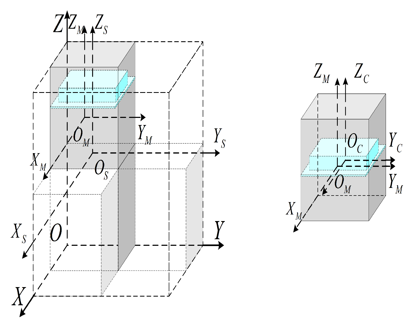
3.1. Coordinate System

The required coordinate system is shown in Figure 2, which includes reference coordinate system, satellite coordinate system, module coordinate system and component coordinate system.

(a) Reference coordinate system. O is the origin of the spatial coordinate system, which is located at the intersection of the bottom of the satellite assembly domain envelope; the $OZ$ axis is the longitudinal axis of the spatial coordinate system, which is vertically upward and positively oriented within the assembly domain composed of the satellite modules; the $OX$ axis, the $OY$ axis and the $OZ$ axis together form a right-handed coordinate system.

(b) Satellite coordinate system. $O_S$ is the origin of the satellite coordinate system, which is located at the geometric center of the outer envelope of satellite. The $O_S{Z}_S$ axis is the satellite’s longitudinal axis, which is vertically upward in the positive direction and parallel to the $OZ$ axis; the $O_S{X}_S$ axis is parallel to the $OX$ axis; the $O_S{Y}_S$ axis is parallel to the $OY$ axis and parallel to the $OX$ axis; the $O_S{X}_S$ axis and the $O_S{Y}_S$ axis form a right-handed coordinate system together with the $O_S{Z}_S$ axis.

(c) Module coordinate system. $O_M$ is the module coordinate system origin, located at the module geometric center. $O_M{Z}_M$ is the module coordinate system vertical axis, which is the same as the layout direction of the module. $O_M{X}_M$ and $O_M{Y}_M$, together with the $O_M{Z}_M$ axis, form a right-handed coordinate system.

(d) Component coordinate system. $O_C$ is the origin of the component coordinate system and is located at the center of mass of the component. $O_C{Z}_C$ is the component longitudinal axis, which is parallel to or coincides with the $O_M{Z}_M$ axis of the module in which it is located. $O_C{X}_C$ is parallel to the $O_M{X}_M$ axis, and $O_C{Y}_C$ is parallel to the $O_M{Y}_M$ axis.

3.2. Optimal Variables

The assembly optimization of a multi-module micro–nano satellite includes the assignment optimization and layout optimization of the components, and the design variables involve the position of the components, the installation angle and the number of the module to which they belong. Assuming that the number of modules is N and the number of components is n, setting $\mathrm{C}=\left\{c_1,c_2,\dots ,c_n\right\}$ to be represented by the optimization variables can be designed in the form of Equation (1):

$$\mathrm{C}=\left\{c_i=\left(x_i,y_i,z_i,{\theta }_i,{\tau }_j\right)|i=1,2\dots ,n,{\tau }_j\in \Gamma \right\}$$

(1)

where $\mathrm{C}$ denotes the set of design variables for the module, $c_i$ denotes the optimization variable for the ith module and $(x_i,y_i,z_i)$ is the positional variable of the component $c_i$ expressed in terms of the center of mass of the component $c_i$. ${\theta }_i$ is the angle variable of the component $c_i$, which is used to describe the mounting angle. The component adopts a rectangular or cylindrical structure. When regarding with the rectangular components, ${\theta }_i$ is taken to be 0 or $\pi /2$. When regarding with the cylindrical components, ${\theta }_i\equiv 0$ when placed vertically, and ${\theta }_i$ takes 0 or $\pi /2$ when placed horizontally. $\Gamma$ is a collection of modules and ${\tau }_{j}j\le N$ is the serial number of the module installed in the component $c_i$, which is described using discrete variables. It should be noted that all the modules involved in the assembly in the paper have unique module serial numbers corresponding to them.

3.3. Assembly Constraints of Components and Modules

(1) Component interference constraints

We do not only need to avoid spatial interference between the components, but we also need to avoid spatial interference between the components and modules. The spatial interference between components includes collision interference and inclusion interference, whose detection conditions are shown in Equation (2).

$$\left\{\begin{array}{c}{P}_{ij}=\left(x_i\le x_j+a_j\right)\left(x_i+a_i\ge x_j\right)\left(y_i\le y_j+b_j\right)\left(y_i+b_i\ge y_j\right)\\ T_{ij}=\left(x_i\le x_j\right)\left(y_i\le y_j\right)\left(x_i+a_i\ge x_j+a_j\right)\left(y_i+b_i\ge y_j+b_j\right)\end{array}\right.$$

(2)

where $\left(x_i,y_i\right)$ and $\left(x_j,y_j\right)$ are the geometric center coordinates of the rectangles $c_i$ and $c_j$, respectively. $\left(a_i,b_i\right)$ and $\left(a_j,b_j\right)$ are the lengths and widths of the rectangles $c_i$ and $c_j$, respectively. In particular, when the cross-section of the component is a circle, $a_i,b_i=2·r_i$ and $a_j,b_j=2·r_j$.

Based on the above detection conditions, the spatial interference constraints are given as Equation (3).

$$\Delta A_{ij}=\left\{\begin{array}{c}1,\mathit{if}{P}_{ij}=1\mathit{or}{T}_{ij}=1\hfill \\ 0,\mathit{otherwise}\hfill \end{array}\right.$$

(3)

where $\Delta A_{ij}=1$ when there is a collision or contained interference, otherwise, $\Delta A_{ij}=0$.

It is necessary to determine the interference between components within the same module, which is expressed by Equation (4):

$$h_{g1}\left(C\right)=\sum _{i=1}^{n-1}\sum _{j=i+1}^n\Delta A_{ij}$$

(4)

Similarly, the relationship of Equation (5) should satisfy the inclusion relationship, i.e., the component does not exceed the envelope of the module.

$$\Delta A_i=\left\{\begin{array}{c}1,\mathit{if}{T}_i=1\hfill \\ 0,\mathit{otherwise}\hfill \end{array}\right.$$

(5)

where the component is contained in the module, and $\Delta A_{ij}$ is 1; otherwise, $\Delta A_{ij}$ is 0.

At this point, it is necessary to determine the inclusion interference of any component with the module, which is expressed through Equation (6):

$$h_{g2}\left(C\right)=\prod _{i=1}^n\Delta A_i$$

(6)

where $h_{g2}\left(C\right)$ denotes the containment non-interference constraints of the component with the module. n denotes the number of components integrated within the module, and $\Delta A_i$ denotes the interference variables of the component with the module.

(2) Module Occupancy Constraints

The integration of components within a module extends along the module assembly direction. Assuming that the axial distance of the integratable space inside the module is $l_M$, the space occupancy constraint of the module can be described by Equation (7):

$$g_o\left(C\right)={\displaystyle \frac{{\displaystyle \sum _{i=1}^n}{d}_i}{l_M}}\times 100$$

(7)

where $g_o\left(C\right)$ denotes the space occupancy constraints within the module; $d_i$ denotes the occupancy space for the integration of the components within the module; and denotes the number of components.

(3) Components function constraints

For some components with specific functions, such as star sensors, sun sensors and payloads, they are required to be mounted in a position that does not affect the field of view. The function constraints can be expressed in Equation (8):

$$F_i=\left\{\begin{array}{c}1,\mathit{if}{p}_i\in P_s\\ 0,\mathit{otherwise}\end{array}\right.$$

(8)

where $F_i$ denotes the functional constraint variables of the component $c_i$; $p_i$ denotes the integration location of the component; and $P_s$ denotes the set of conforming component integration locations.

When the component $c_i$ is integrated to a certain position that meets the design requirements, the value of the functional constraint is 1; otherwise, the value is 0. According to the constraints, the components with specific functions in the satellite system are able to satisfy the functional constraints, which can be shown in Equation (9):

$$h_f\left(C\right)=\prod _{i=1}^n{F}_i$$

(9)

When all the special-function components satisfy the functional constraints, $h_f\left(C\right)=1$; otherwise, $h_f\left(C\right)=0$.

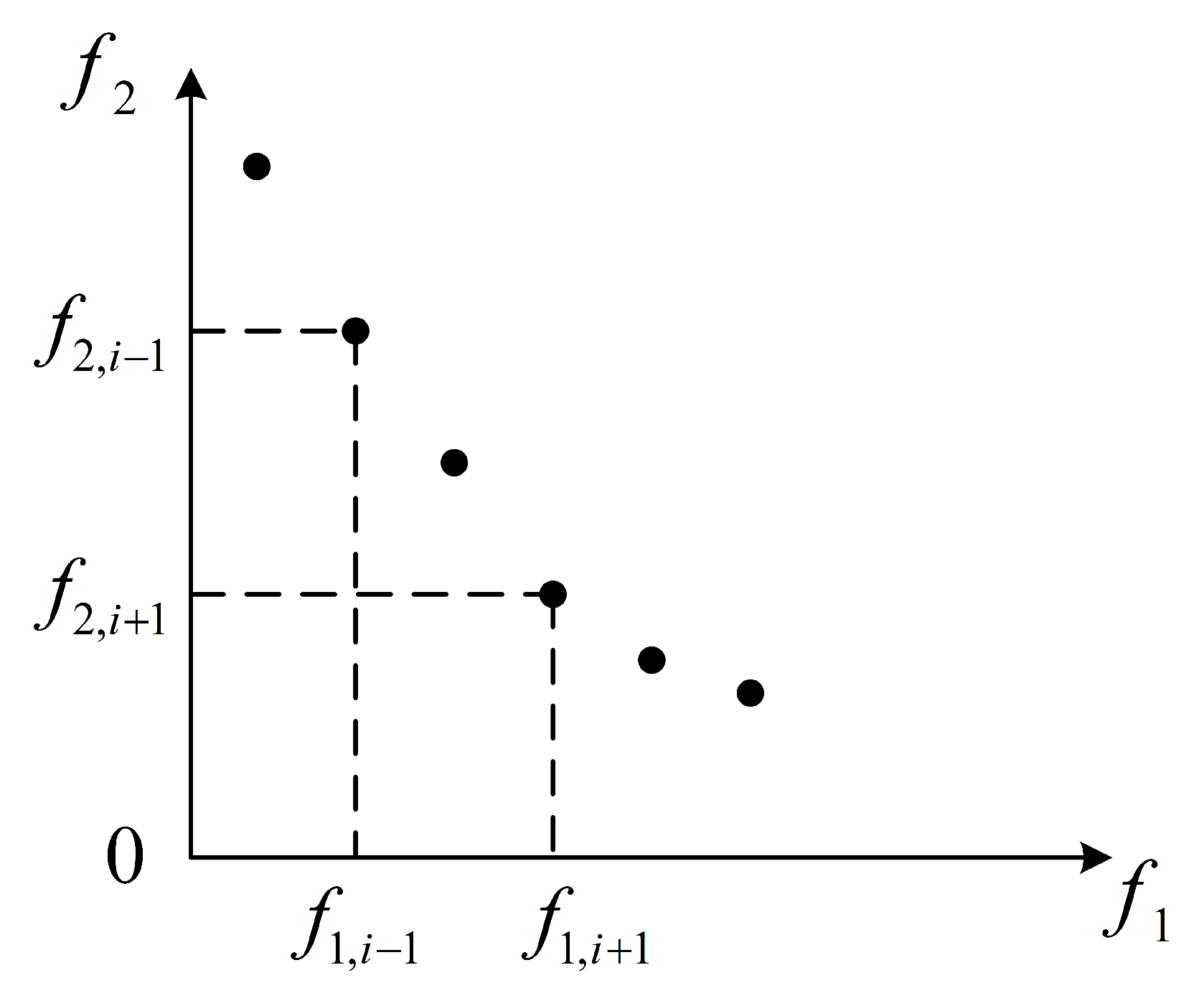
3.4. Objective Functions

The mass characterization objective function includes the mass difference (MD), moment of inertia (MOI) and product of inertia (POI).

(1) Center of mass of satellite

Before solving, the center-of-mass (COM) position of the satellite system needs to be obtained first. The COM of the satellite system is shown in Equation (10):

$$\left\{\begin{array}{c}{x}_m=\left({\displaystyle \sum _{j=1}^N}{M}_j{X}_j+{\displaystyle \sum _{i=1}^n}{m}_i{\widehat{x}}_i\right)/\left({\displaystyle \sum _{j=1}^N}{M}_j+{\displaystyle \sum _{i=1}^n}{m}_i\right)\\ y_m=\left({\displaystyle \sum _{j=1}^N}{M}_j{Y}_j+{\displaystyle \sum _{i=1}^n}{m}_i{\widehat{y}}_i\right)/\left({\displaystyle \sum _{j=1}^N}{M}_j+{\displaystyle \sum _{i=1}^n}{m}_i\right)\\ z_m=\left({\displaystyle \sum _{j=1}^N}{M}_j{Z}_j+{\displaystyle \sum _{i=1}^n}{m}_i{\widehat{z}}_i\right)/\left({\displaystyle \sum _{j=1}^N}{M}_j+{\displaystyle \sum _{i=1}^n}{m}_i\right)\end{array}\right.$$

(10)

where $x_m,y_m,z_m$ denote the COM coordinates of the satellite system; N denotes the number of modules; $M_j$ denotes the mass of the jth module; $X_j,Y_j,Z_j$ denote the center-of-mass coordinates of the module; n denotes the number of components; $m_i$ denotes the mass of the ith component; and $x_i,y_i,z_i$ denote the positional coordinates of the ith component.

(2) Mass difference

The component assignment scheme directly affects the mass difference between modules, which will not only lead to a large shift in the COM position of the satellite, but also interfer with the control torque of the satellite. To describe the mass difference between modules, the mass difference objective function will be expressed by the standard deviation of the module mass.

Considering that the mass of modules with different specifications is not the same, the mass of modules needs to be normalized, and the expression is shown in Equation (11).

$$\overline{M}={\displaystyle \frac{{\displaystyle \sum _{j=1}^N}{k}_j{M}_j}{N}}$$

(11)

where $\overline{M}$ denotes the mean value of the mass of the module; $M_j$ denotes the mass of the jth module; N denotes the number of modules; and $k_j$ denotes the normalization coefficients of the jth module, and according to the module specifications, the normalization coefficients of the 1U, 2U and 3U modules are linearized to configure the coefficients with the ratio of coefficients are 3, 2 and 1.

The standard deviation of the mass of the module can be obtained by solving Equation (12).

$$\tilde{M}\left(S\right)=\sqrt{{\displaystyle \frac{{\displaystyle \sum _{j=1}^N}{\left[k_j·M_j-\overline{M}\right]}^2}{N}}}$$

(12)

where $\tilde{M}S$ denotes the system quality standard deviation.

The mass difference objective function can be described by the mass standard deviation as shown in Equation (13).

$$f_M\left(S\right)=\tilde{M}\left(S\right)$$

(13)

(3) Moment of inertia

The moment of inertia objective function is shown in Equation (14).

$$I\left(S\right)=\sqrt{I_{xx}^2\left(S\right)+I_{yy}^2\left(S\right)+I_{zz}^2\left(S\right)}$$

(14)

The equations for the moment of inertia of components in three directions are shown in Equation (15):

$$\left\{\begin{array}{c}{I}_{xx}\left(S\right)=I_{xx}\left(M\right)+I_{xx}\left(C\right)\\ I_{yy}\left(S\right)=I_{yy}\left(M\right)+I_{yy}\left(C\right)\\ I_{zz}\left(S\right)=I_{zz}\left(M\right)+I_{zz}\left(C\right)\end{array}\right.$$

(15)

where $I\left(S\right)$ denotes the MOI of the satellite system; $I_{xx}\left(S\right),I_{yy}\left(S\right),I_{zz}\left(S\right)$ denote the components of the MOI of the satellite system in the three directions in the stellar coordinate system; $I_{xx}\left(M\right),I_{yy}\left(M\right),I_{zz}\left(M\right)$ denote the MOI of the module in three directions; $I_{xx}\left(C\right),I_{yy}\left(C\right),I_{zz}\left(C\right)$ denote the MOI of the components in the three directions.

The MOI of the module and the components can be obtained by calculating Equation (16) and Equation (17), respectively:

$$\left\{\begin{array}{c}{I}_{xx}\left(M\right)={\displaystyle \sum _{j=1}^N}\left(I_{Y^{\prime },j}+I_{Z^{\prime },j}\right)+{\displaystyle \sum _{j=1}^N}{M}_j\left(Y_j^2+Z_j^2\right)-\left(y_m^2+z_m^2\right){\displaystyle \sum _{j=1}^N}{M}_j\hfill \\ I_{yy}\left(M\right)={\displaystyle \sum _{j=1}^N}\left(I_{X^{\prime },j}+I_{Z^{\prime },j}\right)+{\displaystyle \sum _{j=1}^N}{M}_j\left(X_j^2+Z_j^2\right)-\left(x_m^2+z_m^2\right){\displaystyle \sum _{j=1}^N}{M}_j\hfill \\ I_{zz}\left(M\right)={\displaystyle \sum _{j=1}^N}\left(I_{X^{\prime },j}+I_{Y^{\prime },j}\right)+{\displaystyle \sum _{j=1}^N}{M}_j\left(X_j^2+Y_j^2\right)-\left(x_m^2+y_m^2\right){\displaystyle \sum _{j=1}^N}{M}_j\hfill \end{array}\right.$$

(16)

$$\left\{\begin{array}{c}{I}_{xx}\left(C\right)={\displaystyle \sum _{i=0}^n}\left(I_{x^{″},i}{cos}^2{\theta }_i+I_{y^{″},i}{sin}^2{\theta }_i\right)+{\displaystyle \sum _{i=0}^n}{m}_i\left({\widehat{y}}_i^2+{\widehat{z}}_i^2\right)-\left(y_m^2+z_m^2\right){\displaystyle \sum _{i=0}^n}{m}_i\hfill \\ I_{yy}\left(C\right)={\displaystyle \sum _{i=0}^n}\left(I_{y^{″},i}{cos}^2{\theta }_i+I_{x^{″},i}{sin}^2{\theta }_i\right)+{\displaystyle \sum _{i=0}^n}{m}_i\left({\widehat{x}}_i^2+{\widehat{z}}_i^2\right)-\left(x_m^2+z_m^2\right){\displaystyle \sum _{i=0}^n}{m}_i\hfill \\ I_{zz}\left(C\right)={\displaystyle \sum _{i=0}^n}{I}_{z^{″},i}+{\displaystyle \sum _{i=0}^n}{m}_i\left({\widehat{x}}_i^2+{\widehat{y}}_i^2\right)-\left(x_m^2+y_m^2\right){\displaystyle \sum _{i=0}^n}{m}_i\hfill \end{array}\right.$$

(17)

where $I_{X^{\prime },j},I_{Y^{\prime },j},I_{Z^{\prime },j}$ denote the MOI of the module about the modular coordinate system $O_M{X}_M,O_M{Y}_M,O_M{Z}_M$, respectively; $X_j,Y_j,Z_j$ denote the COM coordinates of the module j, respectively; $x_m,y_m,z_m$ denote the COM coordinates of the satellite system, respectively; $M_j$ denotes the mass of the module j; and N denotes the number of modules; $I_{x^{″},i},I_{y^{″},i},I_{z^{″},i}$ denote the MOI of components i with respect to the component coordinate system $O_C{X}_C,O_C{Y}_C,O_C{Z}_C$, respectively; $x_i,y_i,z_i$ denote the COM coordinates of component i, respectively; ${\theta }_i$ denote the integration direction angle of component; $m_i$ denotes the mass of component i; and n denotes the number of components.

The MOI of the module in the module coordinate system and of the components in the component coordinate system can be solved by using the existing model, and the expressions are shown in Equations (18) and (19).

$$\left\{\begin{array}{c}{I}_{x^{″},i}={\displaystyle \frac{m_i}{12}}\left(b_i^2+h_i^2\right)\\ I_{y^{″},i}={\displaystyle \frac{m_i}{12}}\left(a_i^2+h_i^2\right)\\ I_{z^{″},i}={\displaystyle \frac{m_i}{12}}\left(a_i^2+b_i^2\right)\end{array}\right.$$

(18)

$$\left\{\begin{array}{c}{I}_{x^{″},i}={\displaystyle \frac{m_i}{12}}\left(3r_i^2+h_i^2\right)\hfill \\ I_{y^{″},i}={\displaystyle \frac{m_i}{12}}\left(3r_i^2+h_i^2\right)\hfill \\ I_{z^{″},i}={\displaystyle \frac{m_i}{2}}{r}_i^2\hfill \end{array}\right.$$

(19)

where $m_i$ denotes the mass of component i; $a_i,b_i,h_i$ denote the length, width and height of rectangular component i, respectively; and $r_i,h_i$ denote the radius and height of cylindrical component i, respectively.

According to the above calculation process, the expression of the MOI objective function is obtained as shown in Equation (20).

$$f_I\left(S\right)=I\left(S\right)$$

(20)

(4) Product of inertia

To ensure that the inertia axis does not deviate, the moment of inertia is required to be as close to zero as possible.The product of inertia is shown in Equation (21).

$$\widehat{I}\left(S\right)=\sqrt{I_{xy}^2\left(S\right)+I_{yz}^2\left(S\right)+I_{xz}^2\left(S\right)}$$

(21)

where $\widehat{I}\left(S\right)$ denotes the product of inertia of the satellite system;

$$I_{xy}\left(S\right)I_{yz}\left(S\right)I_{xz}\left(S\right)$$

denote the amount of inertial integrals in different directions.

According to the above calculation process, the expression of the PD objective function is obtained, which is shown as follows:

$$f_P\left(S\right)=\widehat{I}\left(S\right)$$

The product of inertia in three directions are shown in Equation (22):

$$\left\{\begin{array}{c}{I}_{xy}={\displaystyle \sum _{j=1}^N}{M}_j\left(X_j-x_m\right)\left(Y_j-y_m\right)+{\displaystyle \sum _{i=1}^n}{m}_i\left(x_i-x_m\right)\left(y_i-y_m\right)\\ I_{yz}={\displaystyle \sum _{j=1}^N}{M}_j\left(Y_j-y_m\right)\left(Z_j-z_m\right)+{\displaystyle \sum _{i=1}^n}{m}_i\left(y_i-y_m\right)\left(z_i-z_m\right)\\ I_{xz}={\displaystyle \sum _{j=1}^N}{M}_j\left(X_j-x_m\right)\left(Z_j-z_m\right)+{\displaystyle \sum _{i=1}^n}{m}_i\left(x_i-x_m\right)\left(z_i-z_m\right)\end{array}\right.$$

(22)

where $I_{xy}\left(S\right),I_{yz}\left(S\right),I_{xz}\left(S\right)$ denote the products of inertia of the satellite system; N denotes the number of modules; $M_j$ denotes the mass of the module j; $X_j,Y_j,Z_j$ denote the spatial layout position of module j; $x_m,y_m,z_m$ denote the position of COM of the satellite system; n denotes the number of components; $m_i$ denotes the mass of the components; $x_i,y_i,z_i$ denote the spatial layout positions of the components.

3.5. Optimization Model

Combined with the optimal variables, optimization objectives and constraints given above, the satellite assembly optimization mathematical model is shown in Equation (23):

$$\begin{array}{cc}\hfill & min\left[f_M\left(S\right),f_I\left(S\right),f_P\left(S\right)\right]\hfill \\ \hfill & s.t.h_{g1}\left(C\right)=0\hfill \\ \hfill & h_{g2}\left(C\right)=1\hfill \\ \hfill & h_f\left(C\right)=1\hfill \\ \hfill & g_0\left(C\right)-{\tilde{h}}_0<0\hfill \end{array}$$

(23)

where $f_M\left(S\right),f_I\left(S\right),f_P\left(S\right)$ denote the mass difference objective function, the MOI objective function and the POI objective function of the satellite system, respectively. In addition, $h_{g1}\left(C\right)$, $h_{g2}\left(C\right)$, $h_f\left(C\right)$ represent the constraints of components, and $g_0\left(C\right)$ represents the constraints of modules, respectively.

4. Solution Approach

The solution used to solve the optimization of multi-module micro–nano satellite assembly is a hybrid optimization method based on a tabu search (TS) algorithm and a multi-objective differential evolutionary (MODE) algorithm. The optimal assignment scheme is obtained by first planning in which module the components should be integrated. On the basis of this, the installation position and angle of the components in the module are carried out to obtain the optimal layout scheme.

4.1. TS-Based Component Assignment Method

The assignment method matches components with modules and can be used to determine the assignment relationship between components and modules. Component assignment is used to obtain the minimum mass difference ($f_M\left(S\right)$), while satisfying the module space occupancy constraint ($g_0\left(C\right)$). The assignment method includes two stages: initial assignment and reassignment.

(1) Initialization assignment

Initialized assignment is used to generate the first feasible solution set of assignment schemes, which is performed as follows: when $\mathrm{C}=\left\{c_1,c_2,c_3,\dots ,c_n\right\}$ of the components in the assignment, there are N modules to choose from, which means that the above components will be independently assigned to all N modules, and any one assignment scheme will contain one assignment solution $\mathrm{P}=\left\{P_j|j=1,2\dots ,N\right\}$, where $P_j$ denotes the assignment solution of the module j. In this case, for any module j, the internally integrated components can be expressed as follows: $P_j=\left\{c_{ij}\right|i=1,2,\dots \dots n,j=1,2,\dots ,N\}$, where $c_{ij}$ denotes the component i integrated within the module j.

Before a component is assigned to a module, it is necessary to evaluate whether the component satisfies the constraints with the assigned components to decide whether the current assignment operation is still appropriate. For the components that satisfy the constraints, the current assignment solution is obtained and the current mass difference objective function is obtained.

(2) Reassignment

Reassignment is to adjust the attribution relationship between components and modules several times in order to obtain a smaller mass difference objective function. The redistribution of components adopts the form of random assignment, including two operations of component moving and component swapping, which can effectively expand the search scope of the optimal solution field. The realization process is as follows: on the basis of the initialized assignment scheme, one or two modules are randomly selected, and the number of randomly selected modules is used to determine whether the redistribution operation to be performed belongs to the component moving or component swapping.

a. Component moving. If module ${\tau }_j$ is randomly selected, the component moving operation is performed as follows: randomly select a component $c_i$ from any other module ${\tau }_s$ as the component to be moved, and move $c_i$ to the randomly selected module ${\tau }_j$ in it. By solving the satellite mass difference objective function value $f\left(m\right)$ to determine whether the current moving operation is valid, if $f\left(m\right)$ is reduced, then the current moving operation is retained; otherwise, it is necessary to re-select the components and target modules.

b. Component swapping: If module ${\tau }_s$ and ${\tau }_j$ are randomly selected, then the component swapping operation is performed as follows: randomly select one component $c_s$ from the module ${\tau }_s$, and randomly select one component $c_s$ from the module ${\tau }_j$. Component $c_j$ swaps $c_s$ with the module where $c_j$ is located. By solving the satellite mass difference objective function value $f\left(m\right)$ to determine whether the current swapping operation is valid, if $f\left(m\right)$ is reduced, the current swapping operation is retained; otherwise both two target modules and the components need to be re-selected.

It should be noted that each component moving or component swapping operation needs to strictly comply with the constraints; otherwise, the target modules and components need to be re-selected.

(3) Tabu table for component assignment

To prevent from falling into local optimization, the tabu table based on the TS algorithm is designed to save and release the assignment domain solution of components. The tabu table mainly consists of two parts: tabu object and tabu period. The Tabu object is the generated component assignment scheme, i.e., the neighboring domain solution formed after each component moving or swapping; The tabu period is used to specify the tabu algebra of the solutions in the tabu table, and the maximum tabu period is defined as the tabu length, and the minimum value is zero.

In the assignment optimization process, the neighborhood solution generated after each migration or swap operation is taken as a candidate solution and compared with the current optimal solution. If the candidate solution is better than the current solution, it is necessary to further determine whether the candidate solution belongs to the forbidden solution in the tabu table, and if it does not belong to the forbidden solution, the candidate solution is taken as the optimal solution and the tabu table is updated.

The tabu period and tabu length are both specified positive integers. The tabu period is automatically decremented by 1 during each iteration. When the tabu period reaches 0, the tabu solutions in the tabu table can be released.

4.2. MODE-Based Component Layout Method

After component assignment optimization is completed, the type and number of integrated components within the module are known. However, due to the lack of information on the installation location and orientation, it is still necessary to further determine the layout position of components within the module. Component layout optimization is used to solve the optimal MOI and PD objective functions ($f_I\left(S\right)$ and $f_P\left(S\right)$), while also considering the constraints ($h_{g1}\left(C\right)$, $h_{g2}\left(C\right)$, $h_f\left(C\right)$).

(1) Variable decomposition and reconstruction

The layout optimization design variables for the component are

$$X=\left\{X_i=\left(x_i,y_i,z_i,{\theta }_i,{\tau }_j\right)|i=1,2,\dots ,n;{\theta }_i=\left\{0\pi /2;\right\};j=1,2\dots ,N\right\}$$

where $x_i,y_i,z_i$ denote the position coordinates of the component, ${\theta }_i$ denotes the mounting angle of the component and ${\tau }_j$ denotes the module to which the component belongs.

It is easy to know that the layout optimization variables of the component include both continuous variables ($x_i,y_i,z_i$) and discrete variables (${\theta }_i$ and ${\tau }_j$), which are coupled with each other, making optimization solution difficult. To reduce the complexity of the algorithm, the optimization variables are decomposed and reconstructed, and the implementation of the decomposition and reconstruction of the optimization variables is shown in Figure 3.

The decomposed optimization variables can be formed into position variables (continuous variables), angle variables (discrete variables) and assignment variables (discrete variables). By reconstructing each of the three types of variables, the position variable solution set, the angle variable solution set and the distribution variable solution set can be generated. The reconstructed three variables are independent of each other and can be solved in different ways to improve the efficiency of the algorithm. It should be noted that the assignment variable solution set was determined during the assignment optimization design of the components, which is no longer designed during the layout optimization design.

(2) Layout optimization

Let us consider that continuous and discrete variables need to be designed at the same time and two objective functions, MOI and POI, are involved. Therefore, a multi-objective differential evolutionary algorithm is used to optimize the position variables, and a random mutation approach is used to optimize the angle variables. The implementation process of layout optimization for the components is presented as follows:

Step 1: Initialization Layout

The initialization layout is used to generate the initial position population and angle population of the component, and the spatial range of the initial population should cover the entire search area as much as possible. Therefore, randomly generated individuals are needed to generate the initial position population and the initial angle population, as shown in Equation (24) and Equation (25), respectively.

$$X_{i,0}^k=X_{min}^k+rand·(X_{max}^k-X_{min}^k)$$

(24)

$${\theta }_{i,0}^k=\left\{\begin{array}{c}90,\mathit{if}0.5\le P<1\\ 0,\mathit{if}0\le P<0.5\end{array}\right.$$

(25)

where $X_{i,0}^k$ denotes the position variable of individual i of the kth generation population, $X_{max}^k$ and $X_{min}^k$ denote the upper and lower bounds of the range of values of the population, and $rand$ denotes the random number between (0, 1). ${\theta }_{i,0}^k$ denotes the angle variable of the kth generation of population individual i, and P denotes the mutation rate, which takes values in the range of [0, 1].

Step 2: Layout position optimization of components

The position variable optimization of the components is solved using a multi-objective differential evolutionary algorithm, and the optimization process is divided into three stages: difference, crossover and selection. Different from the classical differential evolution algorithm, the multi-objective differential evolution algorithm also adds non-dominated sorting and congestion calculation to select the good individuals. The specific realization process is as follows:

a. Non-dominated ordering

Non-dominated sort is used to obtain the non-dominated relationships of individuals and the implementation process is as follows:

1st step: Set an individual $i=1$ within any population;

2nd step: For all individuals $j=1,2,\dots ,K,j\ne i$, compare the dominance and non-dominance relationships between individuals;

3rd step: If there does not exist any individual $x_j$ that is better than $x_i$, then $x_i$ is labeled as a non-dominated individual;

4th step: Make $i=i+1$ and go to the 2nd step to continue the judgment until all non-dominated individuals are found.

The set of non-dominant individuals obtained through the above steps is the first level of non-dominant stratum of the population. Then, by ignoring these labeled non-dominant individuals (i.e., these individuals are no longer subject to the next round of comparisons) and following the first step to the fourth step, the second level of non-dominant stratum will be obtained, and so on until the non-dominated ordering of the whole population is obtained.

b. Crowding distance calculation

Crowding distance is a reference index for comparing the same individuals of the non-dominated sort, which is expressed by using the distance between the two individuals neighboring each other before and after the individual in the direction of each objective function. The larger the crowding distance is, the greater the degree of adaptation is indicated, and the results obtained are more effective. Taking two objective functions as an example for illustration, the implementation of the crowding distance between these two objective functions is shown in Figure 4.

Assuming that the maximum and minimum values of the objective function $f_1$ in the set of individuals are $max\left(f_1\right)$ and $min\left(f_1\right)$, and the maximum and minimum values of the objective function $f_2$ are $max\left(f_2\right)$ and $min\left(f_2\right)$, then the crowding of the first individual is the same as that in the first individual $max\left(f_2\right)$ and $min\left(f_2\right)$, and the congestion distance of the first individual is calculated as shown in Equation (26):

$$d_i={\displaystyle \frac{f_{1,i+1}-f_{1,i-1}}{max\left(f_1\right)-min\left(f_1\right)}}+{\displaystyle \frac{f_{2,i+1}-f_{2,i-1}}{max\left(f_2\right)-min\left(f_2\right)}}$$

(26)

After the individuals in the population $R^t$ are given a non-dominated ordering and a congestion distance, the next generation of the population $P^{t+1}$ can be selected based on these two metrics. The selection of offspring individuals starts from the set of individuals $F_1$ with sequence value of 1 for the non-dominated ordering, and if the number of individuals in $F_1$ is less than K, all the individuals in $F_1$ are taken as offspring individuals. Subsequently, select the offspring individuals from the set of offspring individuals $F_2$ with sequence value 2; otherwise, the individuals in $F_1$ are sorted according to the crowding distance from the largest to the smallest, and the top K individuals are selected as the offspring individuals.

(3) Differential operator design

Assume that the population size is $Pop$ and the number of iterations is $t_D$. To illustrate the iteration process of the $\tau$ generation population ${\xi }^{\tau }$, the variation strategy adopted in this paper is DE/best/1, and the variation operator is shown in Equation (27).

$${\varsigma }_r^{\tau }={\xi }_{r_{best}}^{\tau }+F\left({\xi }_{r_1}^{\tau }-{\xi }_{r_2}^{\tau }\right)$$

(27)

where ${\varsigma }_r^{\tau }$ denotes the rth row vector of the variant population ${\varsigma }^{\tau }$; ${\xi }_{r_{best}}^{\tau }$ denotes the row vector with the optimal objective function in the population ${\varsigma }^{\tau }$; F is the coefficient of variation, which is determined artificially; ${\xi }_{r_1}^{\tau }$ and ${\xi }_{r_2}^{\tau }$ denote the row vectors of the randomly generated rows and rows, respectively, where $r_1,r_2\in {\mathbb{N}}^{+},r_1\ne r_2$.

(4) Crossover operator design

Perform the crossover operation on each element of ${\varsigma }_r^{\tau }$ and generate a new population after the crossover; the crossover formula is shown in Equation (28):

$${\zeta }_{r,c}^{\tau }=\left\{\begin{array}{c}{\chi }_{r,c}^{\tau },\mathrm{if}c=k\mathrm{or}\mathrm{rand}[0,1]\le P_r\hfill \\ {\xi }_{r,c}^{\tau },\mathrm{otherwise}\hfill \end{array}\right.$$

(28)

where ${\zeta }_{r,c}^{\tau }$, ${\chi }_{r,c}^{\tau }$ and ${\xi }_{r,c}^{\tau }$ denote the cth ${\zeta }_r^{\tau }$, ${\chi }_r^{\tau }$ and ${\xi }_r^{\tau }$ respectively. Column k denotes a randomly chosen column; $\mathrm{rand}[0,1]$ denotes a randomly generated decimal in the $[0,1]$ interval; and $P_r$ is the set crossover probability.

Note that the components are installed along the axial direction of the module, and when randomly selecting populations for crossover, the axial columns need to be selected in conjunction with the assembly direction of the components.

(5) Selection operator design

After completing the mutation and crossover operations, the objective function value of the new population is calculated and the population with a smaller objective function value is selected to participate in the next iteration; the selection operator of the population is shown in Equation (29):

$${\varsigma }_r^{\tau +1}=\left\{\begin{array}{c}{\zeta }_r^{\tau },\mathit{if}f\left({\zeta }_r^{\tau }\right)\le f\left({\varsigma }_r^{\tau }\right)\hfill \\ {\varsigma }_r^{\tau },\mathit{otherwise}\hfill \end{array}\right.$$

(29)

where ${\varsigma }_r^{\tau +1}$ denotes the generated new generation population.

To select good populations as much as possible, the implementation flow process of location layout optimization is specified as follows: (1) initialize the location populations; (2) non-dominated sorting; (3) congestion calculation to screen out the good individuals; (4) perform the difference operation to generate the differential population; (5) perform the crossover operation; and (6) perform the selection operation to screen out the optimal population as the next iteration of the population.

Step 3: Optimization of component mounting angle

The optimization of the angle variable adopts the form of a random mutation; considering that the installation angle is 0 or 90°, the value of the angle variable mainly depends on the range of the mutation rate P, and the specific value is shown in Equation (25).

For the above layout optimization method, the number of iterations is set at first, and the optimization is considered to end when and only when the iteration reaches the upper limit value, and the minimum mass characteristic obtained at this time is the optimal value of the objective function of the mass characteristic, and the corresponding layout scheme is the optimal layout scheme. Finally, the assignment variables, position variables and angle variables are fused to obtain the final optimal assembly optimization design scheme.

5. Case Study

A 12U micro–nano satellite with a defined configuration is used as a simulation case, and to verify the effectiveness of the proposed method.

5.1. Case Description

The 12U micro–nano satellite is an earth observation remote sensing satellite, which is assembled by two 1U modules, two 2U modules and two 3U modules, and the serial numbers of the modules and the corresponding spatial layout are shown in Figure 5.

The coordinates of the space position of each module in the space reference coordinate system are shown in

Table 1. Table of the module spatial location coordinates.

Module Specification	No.	Coordinates
module 1U	u1	(0.0500, 0.0500, 0.2800)
module 2U	u2	(0.1650, 0.1650, 0.2800)
module 3U	u3	(0.0500, 0.0500, 0.1075)
module 1U	u4	(0.1650, 0.1650, 0.1075)
module 2U	u5	(0.1650, 0.0500, 0.1650)
module 3U	u6	(0.0500, 0.1650, 0.1650)
Transfer module 1	u7	(0.1075, 0.0500, 0.2800)
Transfer module 2	u8	(0.1650, 0.1075, 0.2800)
Transfer module 3	u9	(0.1075, 0.1650, 0.2800)
Transfer module 4	u10	(0.0500, 0.1075, 0.2800)
Transfer module 5	u11	(0.0500, 0.0500, 0.2225)
Transfer module 6	u12	(0.1650, 0.1650, 0.2225)
Transfer module 7	u13	(0.1075, 0.0500, 0.1650)
Transfer module 8	u14	(0.1650, 0.1075, 0.1650)
Transfer module 9	u15	(0.1075, 0.1650, 0.1650)
Transfer module 10	u16	(0.0500, 0.1075, 0.1650)
Transfer module 11	u17	(0.1075, 0.0500, 0.0500)
Transfer module 12	u18	(0.1650, 0.1075, 0.0500)
Transfer module 13	u19	(0.1075, 0.1650, 0.0500)
Transfer module 14	u20	(0.0500, 0.1075, 0.0500)

. Considering that the configuration of the satellite has been determined and will not be changed again, it may be assumed that the top surfaces of modules u1, u3, u4 and u6 in the figure are pointing to space, while the bottom surfaces of modules u2, u3, u5 and u6 are oriented to the ground.

A total of 18 components need to be integrated in the satellite, and the parameters of the components are shown in

Table 2. Parameters of components.

No.	Component	Structure	Length/m	Width/m	Height/m	Mass/kg
1	OBC	Cuboid	0.08	0.08	0.04	0.80
2	Battery a	Cuboid	0.07	0.08	0.04	1.10
3	Battery b	Cuboid	0.07	0.08	0.04	1.10
4	Battery c	Cuboid	0.07	0.08	0.04	1.10
5	PCDU	Cuboid	0.07	0.06	0.04	1.00
6	Data storage	Cuboid	0.08	0.08	0.05	0.65
7	TT&C	Cuboid	0.08	0.08	0.05	0.75
8	Camera	Cylinder	0.09		0.09	2.00
9	Star sensor	Cylinder	0.05		0.05	0.45
10	Gyro	Cylinder	0.07		0.04	0.65
11	Sun sensor	Cuboid	0.07	0.08	0.04	0.35
12	Magnetometer	Cuboid	0.07	0.05	0.03	0.60
13	GNSS	Cuboid	0.07	0.06	0.04	0.70
14	Wheel x1	Cuboid	0.08	0.08	0.04	1.80
15	Wheel y1	Cuboid	0.08	0.08	0.04	1.80
16	Wheel z1	Cuboid	0.08	0.08	0.04	1.80
17	Wheel (Standby)	Cuboid	0.08	0.08	0.04	1.80
18	Magnetic torquer	Cuboid	0.05	0.05	0.03	0.50

. These components include 15 rectangular components and 3 cylindrical components. The satellite assembly scheme is required to optimize the mass balance, MOI and POI of the satellite on the basis of satisfying the constraints of space interference, space occupancy constraints and special location.

5.2. Simulation Parameter Setting

(1) TS setting: the number of neighborhood solutions is 200; the tabu length is 12; and the maximum number of iterations is 100. During the iteration process, the component moving and swapping operations are executed separately until the maximum number of iterations is reached.

(2) MODE setting: the population size is $Pop=200$; the variation probability is $F=1.0$; the crossover probability is $P_r=1.0$; the adopted strategy is DE/best/1, and the maximum number of iterations is $t_{Dmax}=5000$. During the iteration process, difference, crossover and selection operations are executed, respectively, until the iteration number is reached.

(3) Evaluation indexes: mass balance of modules $f\left(M\right)$ and Pareto front $f\left(S\right)$ of satellite system mass characteristics, while satisfying the above constraints.

(4) Hardware environment: Intel Core i5-10400F CPU 4.8GHz (Intel, Santa Clara, CA, USA); software operating environment: MATLAB 2023b.

5.3. Constraint Setting

The range of the constraints’ allowable value settings is shown in Table 3.

Table 3. Permitted range for assembly constraints.

Constraints	Description	Permitted Value
Constraints of components	$h_{g1}\left(C\right)={\displaystyle \sum _{i=1}^{n-1}}{\displaystyle \sum _{j=i+1}^n}\Delta A_{ij}$	0
	$h_{g2}\left(C\right)={\displaystyle \prod _{i=1}^n}\Delta A_i$	1
	$h_f\left(C\right)={\displaystyle \prod _{i=1}^n}{F}_i=1$	see Table 4
Constraints of modules	$g_o\left(C\right)={\displaystyle \frac{{\displaystyle \sum _{i=1}^n}{d}_i}{l_M}}\times 100\%$	$\le 80\%$

Table 3. Permitted range for assembly constraints.

Constraints	Description	Permitted Value
Constraints of components	$h_{g1}\left(C\right)={\displaystyle \sum _{i=1}^{n-1}}{\displaystyle \sum _{j=i+1}^n}\Delta A_{ij}$	0
	$h_{g2}\left(C\right)={\displaystyle \prod _{i=1}^n}\Delta A_i$	1
	$h_f\left(C\right)={\displaystyle \prod _{i=1}^n}{F}_i=1$	see Table 4
Constraints of modules	$g_o\left(C\right)={\displaystyle \frac{{\displaystyle \sum _{i=1}^n}{d}_i}{l_M}}\times 100\%$	$\le 80\%$

Table 4. Permitted range for component installation position constraints.

No.	Component	Layout Requirements
9	Camera	Located at the bottom surface of module u2, u3, u5 or u6
10	Star sensor	Located in the top surface of the u1, u3, u4 or u6 module
12	Sun sensor	Located in the top surface of the u1, u3, u4 or u6 module

Table 4. Permitted range for component installation position constraints.

No.	Component	Layout Requirements
9	Camera	Located at the bottom surface of module u2, u3, u5 or u6
10	Star sensor	Located in the top surface of the u1, u3, u4 or u6 module
12	Sun sensor	Located in the top surface of the u1, u3, u4 or u6 module

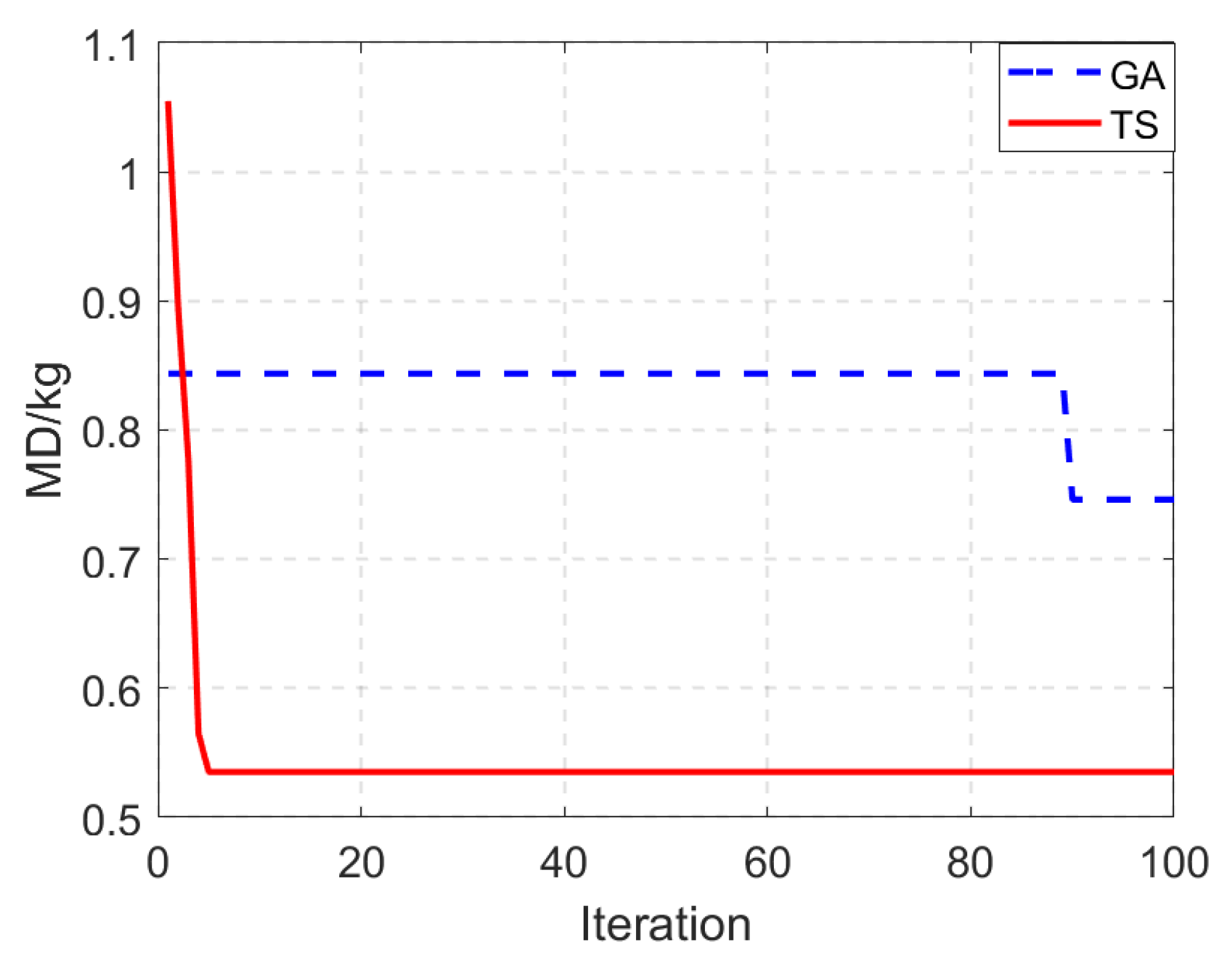
5.4. Results and Analysis

The component assignment problem is handled by initializing the assignment and optimizing the iterative reallocation. All the assignment schemes generated in these two phases are evaluated by the quality difference objective function results of satellite system layout optimization. The proposed algorithm is compared with the classical genetic algorithm and the comparison results are shown in Figure 6. The constraints of component assignment are shown in Figure 7. It can be seen that the proposed method is able to assign the components in a better way, the assignment results satisfy the constraints, the maximum occupancy rate is 0.8 and the minimum occupancy rate is 0.4. At this point, the optimal assignment scheme is shown in Equation (30), and the optimal mass difference objective function is 0.535 kg.

$$\begin{array}{cc}\hfill & u1=\left\{x9\right\}\hfill \\ \hfill & u2=\left\{x2,x4,x6\right\}\hfill \\ \hfill & u3=\left\{x1,x8,x12,x17\right\}\hfill \\ \hfill & u4=\left\{x11,x15\right\}\hfill \\ \hfill & u5=\left\{x5,x7,x16,x18\right\}\hfill \\ \hfill & u6=\left\{x3,x10,x13,x14\right\}\hfill \end{array}$$

(30)

The optimal assignment scheme obtained is used as a reference to carry out the layout optimization. The layout optimization results of the components are identified by the Pareto solution set of MOI and PD. To verify the advantages of the algorithm, the proposed algorithm is compared with NSGA-II and MPSO, and the results are shown in Figure 8. Meanwhile, the minimum MOI and average MOI of the proposed algorithm under different iterations are shown in Figure 9. Taking 2000 iterations as a reference, the optimal layout obtained by the proposed algorithm is shown in

Table 5. Optimal result of component assembly scheme.

No.	x/m	y/m	z/m	$\mathit{\theta }{/}^{°}$	$\mathit{\eta }$
1	0.050	0.050	0.2000	0	u3
2	0.165	0.050	0.1935	90	u2
3	0.165	0.165	0.1844	0	u6
4	0.165	0.050	0.1352	90	u2
5	0.050	0.165	0.1921	0	u5
6	0.165	0.050	0.1920	90	u2
7	0.050	0.165	0.1854	0	u5
8	0.050	0.050	0.1919	0	u3
9	0.165	0.050	0.6690	90	u1
10	0.165	0.165	0.3165	0	u6
11	0.050	0.165	0.3006	90	u4
12	0.050	0.050	0.3170	0	u3
13	0.165	0.165	0.1217	90	u6
14	0.165	0.165	0.1979	0	u6
15	0.050	0.165	0.2549	90	u5
16	0.050	0.165	0.1923	90	u5
17	0.050	0.050	0.1901	0	u3
18	0.050	0.165	0.1403	0	u5

, and the MOI and PD of the satellite are 0.4245 $\mathrm{kg}·{\mathrm{m}}^2$ and 0.01794 $\mathrm{kg}·{\mathrm{m}}^2$.

From the above results, it can be seen that the proposed MODE method can effectively reduce the MOI and PD of the satellite and generate a better Pareto front solution set. Compared to MPSO, the MOI is obviously smaller although it has a larger PD value, while the optimization results of MODE and MPSO are better than NSGA-II both in terms of non-dominance and dispersion. Meanwhile, the solution set obtained by NSGA-II is more dispersed, which is not favorable to the selection of the optimal layout scheme.

Considering that the MOI of micro–nano satellites tends to receive more attention, the MOI under different iterations is simulated, and the average and minimum values of MOI are analyzed. The minimum value of MOI shown in Figure 9 is smaller than the average value under different iterations, which also indicates the effectiveness of the algorithm. However, when facing a bi-objective optimization problem, the selection of the layout scheme also needs to focus on the value of PD, so the optimal solution that satisfies the requirements is not unique, and it can be screened with more practical task requirements.

It can be seen that the proposed method in this paper has a better effect on both the assignment optimization and layout optimization of components, and therefore can be applied to the assembly optimization design problem of the micro–nano satellites.

6. Conclusions

In this paper, a hybrid assembly optimization method is proposed for solving the assembly optimization design problem of a multi-module micro–nano satellite. The TS algorithm obtains the optimal assignment scheme of the components by initializing the assignment and reassignment. On this basis, the MODE algorithm is used to perform the mutation, crossover and selection operations on the components, and the Pareto solution set of each iteration is obtained by non-dominated sorting and crowding calculation. The effectiveness and advantages of the proposed method are verified by simulation, and the results show that the proposed method can be applied to the assembly optimization design problem of multi-module micro–nano satellites with good optimization effect.

References

1. Junichiro, K.; Masahiro, F.; Shinya, F.; Yuji, S.; Toshinori, K.; Kazuya, Y.; Shingo, N.; Kohei, T.; Saki, K.; Kokubo, H. On the low-cost asynchronous one-way range measurement method and the device for micro to nano deep space probes. Acta Astronaut. 2024, 214, 457–465. [Google Scholar]
2. Somov, Y.; Butyrin, S.; Somov, S. Autonomous Control of a Small Spacecraft in Initial Orientation Modes. Ifac-Papersonline 2021, 54, 345–350. [Google Scholar] [CrossRef]
3. Li, X.; Li, X.; Tang, L.; Yang, Z.; Yang, L. Development of a compact solar array drive assembly based on ultrasonic motor for deep space micro-nano satellites. Acta Astronaut. 2025, 228, 865–874. [Google Scholar]
4. Wen, Y.; Xiao, Q.C.; Yong, Z.; Michel, V.T. A Fractionated Spacecraft System Assessment Tool Based on Lifecycle Simulation Under Uncertainty. Chin. J. Aeronaut. 2012, 25, 71–82. [Google Scholar]
5. Ran, D.; Sheng, T.; Cao, L.; Chen, X.; Zhao, Y. Attitude control system design and on-orbit performance analysis of nano-satellite—“Tian Tuo 1”. Chin. J. Aeronaut. 2014, 27, 593–601. [Google Scholar]
6. Yu, X.; Xian, C.; Zhi, L.; Wei, Z.; Wen, Y.; Zhong, Z. Mixed integer programming modeling for the satellite three-dimensional component assignment and layout optimization problem. Chin. J. Aeronaut. 2025, 294, 103415. [Google Scholar]
7. Kortmann, M.; Schervan, A.; Schmidt, H.; Steffen, R.; Kreisel, J. Building Block-based “iBOSS” Approach: Fully Modular Systems with Standard Interface to Enhance Future Satellites. In Proceedings of the 66nd International Astronautical Congress, Jerusalem, Israel, 12–16 October 2015. [Google Scholar]
8. Schervan, A.; Kortmann, M.; Schröder, K.; Kreisel, J. iBOSS Modular Plug & Play - Standardized Building Block Solutions for Future Space Systems Enhancing Capabilities and Flexibility, Design, Architecture and Operations. In Proceedings of the 68th International Astronautical Congress (IAC 2017), Adelaide, Australia, 25–29 September 2017; pp. 9375–9385. [Google Scholar]
9. Schervan, A.; Richert, B.; Zimmermann, J.; Zeis, C.; Häming, M.; Dück, A.; Schröder, K. Assembly and Qualification of a Modular Satellite Structure. In Proceedings of the International Astronautical Congress, Bremen, Germany, 1–5 October 2018; pp. 1–8. [Google Scholar]
10. Chong, Z.; Zhi, X.; Hong, T. Multi-module satellite component assignment and layout optimization. Appl. Soft Comput. 2019, 75, 148–161. [Google Scholar]
11. Teng, H.F.; Sun, S.L.; Liu, D.Q.; Li, Y.Z. Layout optimization for the objects located within a rotating vessel—A three-dimensional packing problem with behavioral constraints. Comput. Oper. Res. 2001, 28, 521–535. [Google Scholar]
12. Juliette, G.; Mathieu, B.; Arnault, T.; Romain, W.; Nouredine, M.; El-Ghazali, T. Hidden-variables genetic algorithm for variable-size design space optimal layout problems with application to aerospace vehicles. Eng. Appl. Artif. Intell. 2023, 121, 105941. [Google Scholar]
13. Sun, G.; Teng, F. Optimal layout design of a satellite module. Eng. Optim. 2003, 35, 513–529. [Google Scholar] [CrossRef]
14. Zhang, B. Particle swarm optimization based on pyramid model for satellite module layout. Chin. J. Mech. Eng. 2005, 4, 530. [Google Scholar] [CrossRef]
15. Lau, W.; Chan, M.; Tsui, T.; Ho, S.; Choy, L. An AI approach for optimizing multi-pallet loading operations. Expert Syst. Appl. 2009, 36, 4296–4312. [Google Scholar] [CrossRef]
16. Grignon, M.; Fadel, M. A GA Based Configuration Design Optimization Method. J. Mech. Des. 2004, 126, 6–15. [Google Scholar] [CrossRef]
17. Fei, T.; Chen, Y.; Zeng, W. A Dual-System Variable-Grain Cooperative Coevolutionary Algorithm: Satellite-Module Layout Design. IEEE Trans. Evol. Comput. 2010, 14, 438–455. [Google Scholar]
18. Xu, Y.C.; Xiao, R.B.; Amos, M. A novel genetic algorithm for the layout optimization problem. In Proceedings of the 2007 IEEE Congress on Evolutionary Computation, Singapore, 25–28 September 2007; Volume 14, pp. 3938–3943. [Google Scholar]
19. Ye, H.; Liang, H.; Yu, T.; Wang, J.; Guo, H. A bi-population clan-based genetic algorithm for heat pipe-constrained component layout optimization. Expert Syst. Appl. 2023, 213, 118881. [Google Scholar]
20. Zhi, X.; Chong, Z.; Hong, T. Assignment and layout integration optimization for simplified satellite re-entry module component layout. Inst. Mech. Eng. Part J. Aerosp. Eng. 2017, 233, 095441001770422. [Google Scholar]
21. Chen, X.; Liu, S.; Sheng, T.; Zhao, Y.; Yao, W. The satellite layout optimization design approach for minimizing the residual magnetic flux density of micro-and nano-satellites. Acta Astronaut. 2019, 163, 299–306. [Google Scholar]
22. Meller, D.; Bozer, A. A new simulated annealing algorithm for the facility layout problem. Int. J. Prod. Res. 1996, 34, 1675–1692. [Google Scholar] [CrossRef]
23. Hong, T.; Ren, S.; Jiang, W.; Xian, C. Optimization of Multi-Objective Unequal Area Facility Layout. IEEE Access 2022, 10, 38870–38884. [Google Scholar]
24. Xian, C.; Wen, Y.; Yong, Z.; Xiao, C.; Wei, L. A novel satellite layout optimization design method based on phi-function. Acta Astronaut. 2021, 180, 560–574. [Google Scholar]
25. Cuco, C.; Sousa, L.; Silva, J. A multi-objective methodology for spacecraft equipment layouts. Optim. Eng. 2015, 16, 165–181. [Google Scholar] [CrossRef]
26. Fakoor, M.; Taghinezhad, M. Layout and configuration design for a satellite with variable mass using hybrid optimization method. Inst. Mech. Eng. Part J. Aerosp. Eng. 2015, 230, 360–377. [Google Scholar] [CrossRef]
27. Fakoor, M.; Seyed, M.; Navid, G.; Hossein, S. Spacecraft Component Adaptive Layout Environment (SCALE): An efficient optimization tool. Adv. Space Res. 2016, 58, 1654–1670. [Google Scholar] [CrossRef]
Figure 1. Three-dimensional structure of the multi-module micro–nano satellite.
Aerospace 12 00614 g001
Figure 2. Coordinate definition of satellite.
Aerospace 12 00614 g002
Figure 3. Implementation of the decomposition and reconstruction of the optimization variables.
Aerospace 12 00614 g003
Figure 4. Implementation of the crowding distance between objective functions.
Aerospace 12 00614 g004
Figure 5. Three-dimensional structure of 12U micro–nano satellite.
Aerospace 12 00614 g005
Figure 6. Optimal result of the mass difference.
Aerospace 12 00614 g006
Figure 7. Occupancy constraint of component assignment.
Aerospace 12 00614 g007
Figure 8. Result of the Pareto solution for different algorithms.
Aerospace 12 00614 g008
Figure 9. Best MOI and mean MOI under different iterations.
Aerospace 12 00614 g009