Two-Stage Uncertain UAV Combat Mission Assignment Problem Based on Uncertainty Theory

Abstract

Based on uncertainty theory, this paper studies the problem of unmanned aerial vehicle (UAV) combat mission assignment under an uncertain environment. First, considering both the target value, which is the combat mission benefit gained from attacking the target, and the unit fuel consumption of UAV as uncertain variables, an uncertain UAV combat mission assignment model is established. And according to decisions under the realization of uncertain variables, the first stage generates an initial mission allocation scheme corresponding to the realization of target value, while the second stage dynamically adjusts the scheme according to the realization of unit fuel consumption; a two-stage uncertain UAV combat mission assignment (TUCMA) model is obtained. Then, because of the difficulty of obtaining analytical solutions due to uncertainty and the complexity of solving the second stage, the TUCMA model is transformed into an expected value-effective deterministic model of the two-stage uncertain UAV combat mission assignment (ETUCMA). A modified particle swarm optimization (PSO) algorithm is designed to solve the ETUCMA model to get the expected value-effective solution of the TUCMA model. Finally, experimental simulations of multiple UAV combat task allocation scenarios demonstrate that the proposed modified PSO algorithm yields an optimal decision with maximum combat mission benefits under a maximum iteration limit, which are significantly greater benefits than those for the mission assignment achieved by the original PSO algorithm. The proposed modified PSO exhibits superior performance compared with the ant colony optimization algorithm, enabling the acquisition of an optimal allocation scheme with greater benefits. This verifies the effectiveness and superiority of the proposed model and algorithm in maximizing combat mission benefits.

1. Introduction

1.1. Motivation

In the modern military field, unmanned aerial vehicles (UAVs) have a very wide range of application due to their remarkable advantages of low cost and complete functionality. UAVs are often used to perform tasks that are dangerous and monotonous for humans. For example, in the event of natural disasters, the harsh environment will make manned aircraft unable to carry out rescue; in the battlefield environment, small-scale multi-target reconnaissance missions are not suitable for manned aircraft to perform. In such circumstances, the utilization of UAVs becomes particularly crucial. However, the fault tolerance rate of single UAV combat is relatively low. Therefore, the clustering of UAVs has become the current development trend, and the task allocation of multi-UAV combat is the key to the application of UAV swarms [1]. Considering the complexity of the actual combat environment, studying the UAV combat mission assignment problem, including constructing its mathematical model, designing solution algorithms, and conducting experimental simulations, while taking into account various factors such as maximum amount of fuel storage, target value, and maximum flight distance, is of great practical significance.

Due to the complexity of the real combat environment of UAVs, that task assignment of UAVs is characterized by uncertainty and changeability. Currently, UAV combat mission assignment models in deterministic environments are not well adapted to the actual battlefield environment. When researching these uncertainties in UAV combat mission assignment problem, many scholars initially regarded them as random factors and conducted studies using mature theoretical systems such as probability theory. However, it is well known that a fundamental prerequisite for applying probability theory is that the estimated probability distribution is close enough to the actual frequency. Given the non-experimental, dynamic, and complex characteristics of factors such as terrain, atmosphere, and temperature in the battlefield environment, the extractable sample size is too small to accurately estimate the probability distribution. Therefore, decision-makers need to invite military professionals to assess the level of belief that each event will happen in uncertainties, which is called uncertainty with expert belief degree. Consequently, dealing with uncertainty with expert belief degree in the UAV combat mission assignment problem to obtain the optimal mission allocation scheme has become the core concern of this field.

Uncertainty theory is an axiomatic mathematical system characterized by normativity, duality, subadditivity, and the product rule, which is used to handle uncertainty with expert belief degree. Based on uncertainty theory, uncertainty factors are regarded as uncertain variables, and each uncertain variable corresponds to a specific uncertainty distribution. Moreover, according to the decision of the occurrence of uncertain variables, a two-stage optimization approach is proposed to construct a two-stage uncertain programming model.

Aiming at these above problems, this paper studies the two-stage uncertain UAV combat mission assignment problem based on uncertainty theory.

1.2. Literature Review

Unmanned aerial vehicle (UAV) technology is moving towards future warfare and becoming a new source of combat effectiveness. Ref. [2] proposed a multi-objective ant colony optimization algorithm with a novel pheromone update mechanism and heuristic information to solve combat mission allocation problem for heterogeneous UAVs in modern military contexts, modeling it as a constrained multi-objective optimization problem. Ref. [3] proposed a two-phase consensus-based group bundling algorithm (CBGBA), which empowers UAVs to achieve consensus on task allocation outcomes in dynamic operational environments. The application of UAVs in the military field is becoming more and more widespread [4] due to their numerous functions and low cost. Most previous studies have usually been conducted in a deterministic environment on the issue of UAV mission allocation. Qadir et al. [5] gave a review of research on UAV mission programming. The studies of these scholars are grounded in deterministic environments that do not fully reflect the uncertainty of realistic battlefield scenarios. In order to be more realistic, people have started to turn to uncertainty, but only to view the uncertainties that arise as random variables and use theoretical knowledge such as probability theory for UAV mission assignment studies.

Primarily, the two-stage optimization approach is a mathematical method for dealing with practical problems that contain random factors, and the mathematical model established for it is known as two-stage stochastic programming. Two-stage stochastic programming is built in such a way that the deviations caused by random factors in the modeling process are compensated for by the second-stage problem, which is more suitable for the actual problem. Therefore, it has been widely used in many fields and has achieved good results. Currently, both theoretical results and applied practices have been developed in stochastic environments. In fact, from the 1950s, Dantzig [6] first applied linear programming to the optimization issue in the number design of airline flights. He took into account that passenger flow is the random variable, and the two-stage stochastic programming model with compensation was first developed. Many studies on two-stage stochastic programming problems have also emerged, such as Shapiro et al. [7] and Jordehi et al. [8]. Due to the difficulty of solving the second-stage problem in two-stage programming, many scholars have studied its solution algorithm. Pasupathy et al. [9] studied problems about two-stage stochastic linear programs by adaptive sequential SAA (sample average approximation) algorithms. In terms of applications, e.g., Irawan et al. [10] studied applications in energy planning problems; additionally, scheduling [11], supply chain network design [12], capacity expansion planning [13], etc., have been studied. Moreover, MacNeil [14] developed a novel approach leveraging binary decision diagrams to solve two-stage stochastic programs with binary recourse and logical linking constraints, enhancing computational efficiency in complex scenarios. Ref. [15] provided a comprehensive review of dynamic task assignment solutions in multi-UAV systems from 2013 to 2024, evaluating algorithms based on responsiveness, robustness, and scalability and identifying key research gaps for future development.

For the military problem of UAV combat mission assignment, the battlefield environment is complex and changeable, and uncertainty with expert belief degree exists everywhere. Regarding such uncertainties, uncertainty theory serves as a robust mathematical system, and there have been numerous studies on both its theoretical foundations and practical applications. For example, in 2007 and 2010, Liu [16,17] proposed and redefined a set of axiomatic mathematical systems: uncertainty theory. In theoretical aspects, Jia [18] showed the tightness of triangle inequality in uncertainty theory; Zeng [19] studied uncertainty theory as a basis for belief reliability. In application aspects, Funfschilling [20] studied the application of uncertainty theory in vehicle speed calculation; Li [21] considered a multi-period portfolio optimization problem under uncertain circumstances based on uncertainty theory; Lio [22] illustrated the Bayesian rule in the framework of uncertainty theory; and Zhang [23] studied the application of uncertainty theory in the optimization process of the routes of customized buses. Both theoretical developments and practical applications in this field have accumulated a wealth of the literature, demonstrating the effectiveness and applicability of uncertainty theory in addressing complex real-world problems.

However, the research on two-stage uncertain programming proposed by the two-stage optimization approach is almost non-existent. Therefore, the research on the two-stage uncertain UAV combat mission assignment problem based on uncertainty theory has broad prospects and use value.

1.3. Proposed Approaches

Maximizing mission benefits remains a critical challenge in the UAV combat mission assignment problem. Due to the incomplete and imprecise information about the target mission, the target value is modeled as an uncertain variable. And fuel consumption is also an uncertain variable, owing to the fact that the navigation speed of UAVs is not constant and is influenced by the terrain environment. When considering the completion of an attack mission, the goal is to obtain the maximum total value of targets. Now, it is assumed that the target value can be obtained by attacking the target, and the case where the target is attacked but not taken down is ignored. How should UAVs be optimally allocated to maximize the obtained target values? First, we establish an uncertain UAV combat mission assignment (UCMA) model. And, based on the decisions made by the occurrence of uncertain variables, a two-stage uncertain UAV combat mission assignment (TUCMA) model is established by using the two-stage optimization approach. Then, since the second-stage problem of the TUCMA model is difficult to solve, and these uncertain variables cannot be directly compared, we transform the TUCMA model into an expected value-effective deterministic model of two-stage uncertain UAV combat mission assignment (ETUCMA). A well-designed modified particle swarm optimization (PSO) algorithm is used to solve the ETUCMA model to get the expected value-effective solution of TUCMA model. Finally, examples are applied to obtain the optimal allocation scheme.

This paper is arranged as follows: The next Section 2 gives some information on uncertainty theory related to the paper, mainly including the properties of inverse uncertainty distribution and the concept and properties of the expected values of uncertain variables. Section 3 studies the uncertain UAV combat mission assignment problem based on uncertainty theory. First, based on uncertainty theory, an uncertain UAV combat mission assignment (UCMA) model with uncertain target value and uncertain fuel consumption is constructed. And based on the decisions made by the occurrence of uncertain variables, this UCMA model is handled by a two-stage optimization approach with more compensation for more attacks. A two-stage uncertain UAV combat mission assignment (TUCMA) model is established. Then, the TUCMA model is transformed to find the expected value-effective solution. Finally, an effective modified PSO algorithm is designed for the two-stage programming. Section 4 introduces the modified PSO algorithm in detail. Section 5 gives examples and then verifies the effectiveness and superiority of the proposed model and algorithm. Section 6 gives a summary.

2. Preliminaries

In 2007 and 2010, Liu [16,17] proposed and redefined a set of axiomatic mathematical systems with normative, dual, subadditive, and product axioms: uncertainty theory. The following describes the relevant theorems that will be used in this article. Let $\mathrm{\Gamma }$ be a nonempty set, and let $\mathcal{L}$ be a $\sigma$-algebra over $\mathrm{\Gamma }$. Each element, $\mathrm{\Lambda }$, in $\mathcal{L}$ is called an event. The set function $\mathcal{M}$ is called an uncertain measure if it satisfies the following four axioms [16]: the normality axiom, duality axiom, subadditivity axiom, and product axiom. Then the triplet $(\mathrm{\Gamma },\mathcal{L},\mathcal{M})$ is called an uncertainty space.

Definition 1

([16]). An uncertain variable is a function, ξ, from an uncertainty space, $(\mathrm{\Gamma },\mathcal{L},\mathcal{M})$, to the set of real numbers such that $\left\{\xi \in B\right\}$ is an event for any Borel set, B, of real numbers.

Definition 2

([16]). The uncertainty distribution Φ of an uncertain variable ξ, is defined by

$$\Phi \left(x\right)=\mathcal{M}\left\{\xi \le x\right\}$$

(1)

for any real number, x.

Definition 3

([16]). The distribution function of the uncertain variable ξ, is the following zigzag uncertainty distribution:

$$\Phi \left(x\right)=\left\{\begin{array}{cc}0,& x\le a;\\ {\displaystyle \frac{(x-a)}{2(b-a)}},& a\le x\le b;\\ {\displaystyle \frac{x+c-2b}{2(c-b)}},& b\le x\le c;\\ 1,& x\ge c.\end{array}\right.$$

Then, ξ is a zigzag uncertainty variable, denoted as $\xi \sim Z(a,b,c)$, where a, b, and c are all real numbers and $a<b<c$.

Definition 4

([17]). An uncertain variable ξ, is called normal if it has a normal uncertainty distribution,

$$\Phi \left(x\right)={\left(1+e^{{\displaystyle \frac{\pi \left(e-x\right)}{\sqrt{3}\sigma }}}\right)}^{-1},x\in \Re$$

(2)

denoted by $\mathcal{N}\left(e,\sigma \right)$, where e and σ are real numbers with $\sigma >0$. A normal uncertainty distribution is called standard if $e=0$ and $\sigma =1$.

Definition 5

([17]). Let ξ be an uncertain variable with the regular uncertainty distribution Φ. Then, the inverse function ${\Phi }^{-1}$, is called the inverse uncertainty distribution of ξ.

Theorem 1

([17]). Let ${\eta }_1,\cdots {\eta }_m$ be independent uncertain variables with the regular uncertainty distributions ${\Phi }_1,{\Phi }_2,\cdots {\Phi }_m$, respectively. If $f(x_1,x_2,\cdots ,x_m)$ is continuous, strictly increasing with respect to $x_1,x_2,\cdots ,x_n$ and strictly decreasing with respect to $x_{n+1},x_{n+2},\cdots ,x_m$, then

$$\xi =f\left({\eta }_1,{\eta }_2,\cdots {\eta }_m\right)$$

(3)

has an inverse uncertainty distribution:

$${\mathrm{\Psi }}^{-1}\left(\alpha \right)=f\left({\Phi }_1^{-1}\left(\alpha \right),\cdots ,{\Phi }_n^{-1}\left(\alpha \right),{\Phi }_{n+1}^{-1}\left(1-\alpha \right),\cdots ,{\Phi }_m^{-1}\left(1-\alpha \right)\right).$$

(4)

Theorem 2

([17]). Let η be an uncertain variable with the regular uncertainty distribution Φ. Then,

$$E\left[\eta \right]={\int }_0^1{\Phi }^{-1}\left(\alpha \right)d\alpha .$$

(5)

Theorem 3

([17]). Let η and ξ be independent uncertain variables with finite expected values. Then, for any real numbers, c and d, we have

$$E\left[c\eta +d\xi \right]=cE\left[\eta \right]+dE\left[\xi \right].$$

(6)

3. The Uncertain UAV Combat Mission Assignment Problem

3.1. Problem Description

There is a UAV combat system in place, with our base storing n UAVs that need to attack m enemy mission targets. Assuming that no multiple UAVs attack the same target, the target value is acquired by attacking a mission target, and situations involving failure to hit the target are disregarded. Here, we set up the decision variable $x_{(i,j)}^k$, which indicates whether the k-th UAV attacks the task along the directional trajectory $(i,j)$, which is the path from the i-th target to the j-th target.

$$x_{(i,j)}^k=\left\{\begin{array}{c}1,\mathrm{the}\mathrm{task}\mathrm{is}\mathrm{attacked}\mathrm{by}k\text{-}\mathrm{th}\mathrm{UAV}\mathrm{along}\mathrm{the}\mathrm{trajectory}(i,j);\hfill \\ 0,\mathrm{the}\mathrm{task}\mathrm{is}\mathrm{not}\mathrm{attacked}\mathrm{by}k\text{-}\mathrm{th}\mathrm{UAV}\mathrm{along}\mathrm{the}\mathrm{trajectory}(i,j).\hfill \end{array}\right.$$

(7)

where $k=1,2,\dots ,n$, $i=0,1,2,\dots ,m;j=0,1,2,\dots ,m$.

If a UAV is to depart for an attack mission, it departs from our base. The base is set as the 0-th target. We need to attack as many mission targets as possible under the limits of different flight distances and the different maximum fuel storage of these different UAVs to obtain the maximum target values. However, due to the uncertainties of the terrain and meteorological activities, the UAV combat mission assignment problem becomes extremely complex. The distance from the UAV to the mission target is given. But due to the influence of the terrain environment, the flight speed of the UAV is not constant, which in turn leads to uncertainties in fuel consumption. The fuel consumption is set as an uncertain variable. In the uncertainty theory system, an uncertain factor is referred to as an uncertain variable, which has a corresponding uncertainty distribution. In specific problems, the type of uncertainty distribution that an uncertain variable follows is typically determined by the experience of domain experts. In many cases, these uncertain variables might be assumed to follow a normal uncertainty distribution. The choice of this distribution is based on experts’ understanding of the nature of uncertainty within their field and past experiences, reflecting a consensus or preference among experts regarding the characteristics of uncertainty. Moreover, due to the incomplete and inaccurate information obtained about mission targets, the target value is also an uncertain variable.

3.2. Formulation of Objective Function

The distance between the i-th target and the j-th target is the scalar, denoted by $d_{(i,j)}$. We set the target value of the j-th target as an uncertain variable, ${\eta }_j$, and let ${\Phi }_{{\eta }_j}$ be its uncertainty distribution, $\eta ={({\eta }_1,{\eta }_2,\dots ,{\eta }_m)}^T$ here. Our objective is to obtain the maximum target values, formulated as

$$\underset{x}{max}\sum _{k=1}^n\sum _{i=0}^m\sum _{{\displaystyle \genfrac{}{}{0pt}{}{j\ne i\hfill }{j=1\hfill }}}^m{\eta }_j{x}_{(i,j)}^k;$$

(8)

which is equivalent to the minimum loss

$$\underset{x}{min}-\sum _{k=1}^n\sum _{i=0}^m\sum _{{\displaystyle \genfrac{}{}{0pt}{}{j\ne i\hfill }{j=1\hfill }}}^m{\eta }_j{x}_{(i,j)}^k.$$

(9)

3.3. Establishment of Constraints

3.3.1. Technical Nature Limits of UAVs

In the actual battlefield environment, UAVs have a maximum flight distance, denoted by $D_k$ for the k-th UAV, where $k=1,2,\dots ,n$. UAVs also face fuel capacity limitations, where the maximum fuel storage of the k-th UAV is constrained by $F_k$, $k=1,2,\dots ,n$. We model the fuel consumption as an uncertain variable, ${\xi }_k$, representing the fuel consumption per unit distance for the k-th UAV, and let ${\Phi }_{{\xi }_k}$ denote the corresponding uncertainty distribution of ${\xi }_k$, with $\xi ={({\xi }_1,{\xi }_2,\dots ,{\xi }_n)}^T$.

$$\sum _{j=1}^m\sum _{{\displaystyle \genfrac{}{}{0pt}{}{i\ne j\hfill }{i=0\hfill }}}^m{d}_{(i,j)}{\xi }_k{x}_{(i,j)}^k\le F_k,k=1,2,\dots ,n;$$

(10)

$$\sum _{j=1}^m\sum _{{\displaystyle \genfrac{}{}{0pt}{}{i\ne j\hfill }{i=0\hfill }}}^m{d}_{(i,j)}{x}_{(i,j)}^k\le D_k,k=1,2,\dots ,n.$$

(11)

3.3.2. Constraints on UAV Combat Mission Assignment

After completing attack missions, UAVs are not required to return to our base.

$$\sum _{i=1}^m{x}_{(i,0)}^k=0,k=1,2,\dots ,n.$$

(12)

Each target can be attacked by at most one UAV, and multiple UAVs cannot attack the same target. In the uncertain UAV combat mission assignment problem, it is assumed that the target is destroyed and target value is obtained once the target is attacked.

$$\sum _{k=1}^n\sum _{{\displaystyle \genfrac{}{}{0pt}{}{j\ne i\hfill }{i=0\hfill }}}^m{x}_{(i,j)}^k\le 1,j=1,2,\dots ,m.$$

(13)

The attack path cannot appear as a loop; that is, if the target is attacked by the k-th UAV along the trajectory $(i,j)$, there is no attack path along the trajectory $(j,i)$.

$$\sum _{k=1}^n(x_{(i,j)}^k+x_{(j,i)}^k)\le 1,j=0,1,2,\dots ,m,i=0,1,2,\dots ,m,j\ne i.$$

(14)

The mission sequence executed by a single UAV should form a path, free of overlaps or breakpoints. Therefore, we formulate the following constraints:

$$\sum _{{\displaystyle \genfrac{}{}{0pt}{}{j\ne i\hfill }{j=1\hfill }}}^m{x}_{(i,j)}^k=z_{ki},i=0,1,2,\dots ,m,k=1,2,\dots ,n;$$

(15)

$$\sum _{{\displaystyle \genfrac{}{}{0pt}{}{i\ne j\hfill }{i=0\hfill }}}^m{x}_{(i,j)}^k=z_{kj},j=1,2,\dots ,m,k=1,2,\dots ,n.$$

(16)

where,

$$z_{ki}=\left\{\begin{array}{c}1,\mathrm{the}\mathrm{task}\mathrm{for}i\text{-}\mathrm{th}\mathrm{target}\mathrm{is}\mathrm{attacked}\mathrm{by}k\text{-}\mathrm{th}\mathrm{UAV};\hfill \\ 0,\mathrm{the}\mathrm{task}\mathrm{for}i\text{-}\mathrm{th}\mathrm{target}\mathrm{is}\mathrm{not}\mathrm{attacked}\mathrm{by}k\text{-}\mathrm{th}\mathrm{UAV}.\hfill \end{array}\right.$$

In particular, if $i=0$, we have ${\displaystyle \sum _{{\displaystyle \genfrac{}{}{0pt}{}{j\ne i\hfill }{j=1\hfill }}}^m}{x}_{(0,j)}^k=z_{k0}=1$, indicating the k-th UAV departing from our base.

3.4. The Two-Stage Uncertain UAV Combat Mission Assignment (TUCMA) Model

Based on the previously described objective function and constraints, the uncertain UAV combat mission assignment (UCMA) model is established as follows:

$$\left\{\begin{array}{cc}\underset{x,z}{min}\hfill & -{\displaystyle \sum _{k=1}^n}{\displaystyle \sum _{i=0}^m}{\displaystyle \sum _{{\displaystyle \genfrac{}{}{0pt}{}{j\ne i\hfill }{j=1\hfill }}}^m}{\eta }_j{x}_{(i,j)}^k\hfill \\ \mathrm{s}.\mathrm{t}\hfill & {\displaystyle \sum _{j=1}^m}{\displaystyle \sum _{{\displaystyle \genfrac{}{}{0pt}{}{i\ne j\hfill }{i=0\hfill }}}^m}{d}_{(i,j)}{\xi }_k{x}_{(i,j)}^k\le F_k,k=1,2,\dots ,n,\hfill \\ \hfill & {\displaystyle \sum _{j=1}^m}{\displaystyle \sum _{{\displaystyle \genfrac{}{}{0pt}{}{i\ne j\hfill }{i=0\hfill }}}^m}{d}_{(i,j)}{x}_{(i,j)}^k\le D_k,k=1,2,\dots ,n,\hfill \\ \hfill & {\displaystyle \sum _{i=1}^m}{x}_{(i,0)}^k=0,k=1,2,\dots ,n,\hfill \\ \hfill & {\displaystyle \sum _{k=1}^n}{\displaystyle \sum _{{\displaystyle \genfrac{}{}{0pt}{}{i\ne j\hfill }{i=0\hfill }}}^m}{x}_{(i,j)}^k\le 1,j=1,2,\dots ,m,\hfill \\ \hfill & {\displaystyle \sum _{k=1}^n}(x_{(i,j)}^k+x_{(j,i)}^k)\le 1,j=0,1,2,\dots ,m,i=0,1,2,\dots ,m,j\ne i,\hfill \\ \hfill & {\displaystyle \sum _{{\displaystyle \genfrac{}{}{0pt}{}{j\ne i\hfill }{j=1\hfill }}}^m}{x}_{(i,j)}^k=z_{ki},i=0,1,2,\dots ,m,k=1,2,\dots ,n,\hfill \\ \hfill & {\displaystyle \sum _{{\displaystyle \genfrac{}{}{0pt}{}{i\ne j\hfill }{i=0\hfill }}}^m}{x}_{(i,j)}^k=z_{kj},j=1,2,\dots ,m,k=1,2,\dots ,n,\hfill \\ \hfill & x_{(i,j)}^k\in \{0,1\},z_{ki}\in \{0,1\},j=0,1,\dots ,m,i=0,1,\dots ,m,k=1,2,\dots ,n.\hfill \end{array}\right.$$

(17)

For the $\left(\mathrm{UCMA}\right)$ model, we can consider balancing the losses caused by attacking multiple targets against the remediation costs required to mitigate these losses, aiming to maximize the total target values, that is, the two-stage optimization approach. This approach stems from the fact that the initial decision-making phase does not fully account for the specific characteristics of uncertain variables, leading to inevitable decision deviations once the uncertainty distributions of these variables are later revealed. To compensate for such deviations, an additional stage, namely the second stage, is introduced for corrective refinement.

And according to decisions under the realization of uncertain variables, the first stage generates an initial mission allocation scheme corresponding to the realization of target value, while the second stage dynamically adjusts the scheme according to the realization of unit fuel consumption. Given the complex and changing battlefield environment, attacking all targets may lead to fuel depletion, preventing return to base, or insufficient ammunition resulting in UAV damage. Therefore, a fuel replenishment mechanism must be considered. We know that fuel storage has a limit, but when the fuel storage on the UAV runs out, the emergency fuel reserves pre-allocated for the aircraft can be activated, or aerial refueling can be carried out. However, this mechanism is only activated as a last resort under extreme emergencies, as its activation permanently scraps the UAV and consumes the cost value of the spare fuel. Therefore, we do not emphasize that UAVs must return to base. If a UAV has remaining fuel after completing its mission, it is assumed by default that it can return to base. However, if the UAV completes the mission by activating emergency fuel reserves, it will be permanently scrapped and unable to return to base. Assuming that the k-th UAV exceeds its fuel storage limit, each additional target attack incurs both fuel replenishment costs and aircraft damage costs which are denoted by $T_k$. The final loss is set as $\phi (x,\xi )$. Accordingly, the following two-stage uncertain UAV combat mission assignment $\left(\mathrm{TUCMA}\right)$ model is formulated:

$$\left\{\begin{array}{cc}\underset{x,z}{min}\hfill & -{\displaystyle \sum _{k=1}^n}{\displaystyle \sum _{i=0}^m}{\displaystyle \sum _{{\displaystyle \genfrac{}{}{0pt}{}{j\ne i\hfill }{j=1\hfill }}}^m}{\eta }_j{x}_{(i,j)}^k+E_{\xi }\left[\phi (x,\xi )\right]\hfill \\ \mathrm{s}.\mathrm{t}\hfill & {\displaystyle \sum _{j=0}^m}{\displaystyle \sum _{{\displaystyle \genfrac{}{}{0pt}{}{i\ne j\hfill }{i=0\hfill }}}^m}{d}_{(i,j)}{x}_{(i,j)}^k\le D_k,k=1,2,\dots ,n,\hfill \\ \hfill & {\displaystyle \sum _{i=1}^m}{x}_{(i,0)}^k=0,k=1,2,\dots ,n,\hfill \\ \hfill & {\displaystyle \sum _{k=1}^n}{\displaystyle \sum _{{\displaystyle \genfrac{}{}{0pt}{}{i\ne j\hfill }{i=0\hfill }}}^m}{x}_{(i,j)}^k\le 1,j=1,2,\dots ,m,\hfill \\ \hfill & {\displaystyle \sum _{k=1}^n}(x_{(i,j)}^k+x_{(j,i)}^k)\le 1,j=0,1,2,\dots ,m,i=0,1,2,\dots ,m,j\ne i,\hfill \\ \hfill & {\displaystyle \sum _{{\displaystyle \genfrac{}{}{0pt}{}{j\ne i\hfill }{j=1\hfill }}}^m}{x}_{(i,j)}^k=z_{ki},k=1,2,\dots ,n,i=0,1,2,\dots ,m,\hfill \\ \hfill & {\displaystyle \sum _{{\displaystyle \genfrac{}{}{0pt}{}{i\ne j\hfill }{i=0\hfill }}}^m}{x}_{(i,j)}^k=z_{kj},k=1,2,\dots ,n,j=1,2,\dots ,m,\hfill \\ \hfill & x_{(i,j)}^k\in \{0,1\},z_{ki}\in \{0,1\},j=0,1,\dots ,m,i=0,1,\dots ,m,k=1,2,\dots ,n.\hfill \end{array}\right.$$

(18)

where $\eta ={({\eta }_1,{\eta }_2,\dots ,{\eta }_m)}^T$, $\xi ={({\xi }_1,{\xi }_2,\dots ,{\xi }_n)}^T$, $x=\left(x_{(i,j)}^k\right)$. And

$$\xi \left(\gamma \right)={({\xi }_1\left({\gamma }_1\right),{\xi }_2\left({\gamma }_2\right),\dots ,{\xi }_n\left({\gamma }_n\right))}^T$$

is the realization of the uncertain variable vector $\xi$. The final loss function $\phi (x,\xi )$ is the optimal value of the second-stage problem. The following model is the second-stage problem:

$$\left\{\begin{array}{c}\begin{array}{c}\underset{y,w}{min}\begin{array}{c}c{\displaystyle \sum _{k=1}^n}{\displaystyle \sum _{j=1}^m}{\displaystyle \sum _{{\displaystyle \genfrac{}{}{0pt}{}{i\ne j\hfill }{i=0\hfill }}}^m}{d}_{(i,j)}{\xi }_k\left({\gamma }_k\right)(1-y_{(i,j)}^k)x_{(i,j)}^k\hfill \end{array}\hfill \\ +{\displaystyle \sum _{k=1}^n}\mathrm{sgn}\left({\displaystyle \sum _{j=1}^m}{\displaystyle \sum _{{\displaystyle \genfrac{}{}{0pt}{}{i\ne j\hfill }{i=0\hfill }}}^m}(1-y_{(i,j)}^k)x_{(i,j)}^k\right)T_k\hfill \end{array}\hfill \\ \mathrm{s}.\mathrm{t}\begin{array}{c}{\displaystyle \sum _{j=1}^m}{\displaystyle \sum _{{\displaystyle \genfrac{}{}{0pt}{}{i\ne j\hfill }{i=0\hfill }}}^m}{d}_{(i,j)}{\xi }_k\left({\gamma }_k\right)y_{(i,j)}^k{x}_{(i,j)}^k\le F_k,k=1,2,\dots ,n,\hfill \end{array}\hfill \\ \begin{array}{c}{\displaystyle \sum _{{\displaystyle \genfrac{}{}{0pt}{}{j\ne i\hfill }{j=1\hfill }}}^m}{x}_{(i,j)}^k{y}_{(i,j)}^k=w_{ki},i=0,1,2,\dots ,m,k=1,2,\dots ,n,\hfill \\ {\displaystyle \sum _{{\displaystyle \genfrac{}{}{0pt}{}{i\ne j\hfill }{i=0\hfill }}}^m}{x}_{(i,j)}^k{y}_{(i,j)}^k=w_{kj},j=1,2,\dots ,m,k=1,2,\dots ,n,\hfill \end{array}\hfill \\ y_{(i,j)}^k\in \{0,1\},j=0,1,\dots ,m,i=0,1,\dots ,m,k=1,2,\dots ,n.\hfill \end{array}\right.$$

where the value per unit fuel is denoted by c, which is a constant. We set $\phi (x,\xi )={\displaystyle \sum _{k=1}^n}{\phi }_k(x^k,{\xi }_k),x^k={\left(x_{(i,j)}^k\right)}_{(i,j)}.$

$$w_{ki}=\left\{\begin{array}{cc}1,\hfill & \mathrm{the}\mathrm{task}\mathrm{for}i\text{-}\mathrm{th}\mathrm{target}\mathrm{is}\mathrm{attacked}\mathrm{by}k\text{-}\mathrm{th}\mathrm{UAV}\hfill \\ & \mathrm{when}\mathrm{satisfy}\mathrm{the}\mathrm{fuel}\mathrm{consumption}\mathrm{constraint};\hfill \\ 0,\hfill & \mathrm{otherwise}.\hfill \end{array}\right.$$

The decision made in the first stage directly impacts the second stage, which dynamically adjusts based on changes from the first stage. In simpler terms, each decision, x, in the first stage corresponds to a minimum loss value, $\phi (x,\xi )$, in the second stage. Since uncertain variables cannot be compared directly, we calculate $E_{\xi }\left[\phi (x,\xi )\right]$ for comparison.

And for the TUCMA model, ${\eta }_j(j=1,2,\dots ,m)$ is an uncertain variable, so

$$-\sum _{k=1}^n\sum _{i=0}^m\sum _{{\displaystyle \genfrac{}{}{0pt}{}{j\ne i\hfill }{j=1\hfill }}}^m{\eta }_j{x}_{(i,j)}^k+E_{\xi }\left[\phi (x,\xi )\right]$$

is an uncertain variable. Similarly, the uncertain variables cannot be compared directly. In order to solve the TUCMA model, we take the expected value

$$E[-\sum _{k=1}^n\sum _{i=0}^m\sum _{{\displaystyle \genfrac{}{}{0pt}{}{j\ne i\hfill }{j=1\hfill }}}^m{\eta }_j{x}_{(i,j)}^k+E_{\xi }\left[\phi (x,\xi )\right]]=E_{\eta }[-\sum _{k=1}^n\sum _{i=0}^m\sum _{{\displaystyle \genfrac{}{}{0pt}{}{j\ne i\hfill }{j=1\hfill }}}^m{\eta }_j{x}_{(i,j)}^k]+E_{\xi }\left[\phi (x,\xi )\right].$$

Thus, the TUCMA model is transformed as the following ETUCMA model:

$$\left\{\begin{array}{c}\underset{x,z}{min}\begin{array}{c}\end{array}{E}_{\eta }[-{\displaystyle \sum _{k=1}^n}{\displaystyle \sum _{i=0}^m}{\displaystyle \sum _{{\displaystyle \genfrac{}{}{0pt}{}{j\ne i\hfill }{j=1\hfill }}}^m}{\eta }_j{x}_{(i,j)}^k]+E_{\xi }\left[\phi (x,\xi )\right]\hfill \\ \mathrm{s}.\mathrm{t}\begin{array}{c}{\displaystyle \sum _{j=0}^m}{\displaystyle \sum _{{\displaystyle \genfrac{}{}{0pt}{}{i\ne j\hfill }{i=0\hfill }}}^m}{d}_{(i,j)}{x}_{(i,j)}^k\le D_k,k=1,2,\dots ,n,\hfill \end{array}\hfill \\ \begin{array}{c}{\displaystyle \sum _{i=1}^m}{x}_{(i,0)}^k=0,k=1,2,\dots ,n, \hfill \\ {\displaystyle \sum _{k=1}^n}{\displaystyle \sum _{{\displaystyle \genfrac{}{}{0pt}{}{i\ne j\hfill }{i=0\hfill }}}^m}{x}_{(i,j)}^k\le 1, j=1,2,\dots ,m,\hfill \\ {\displaystyle \sum _{k=1}^n}(x_{(i,j)}^k+x_{(j,i)}^k)\le 1, j=0,1,2,\dots ,m,i=0,1,2,\dots ,m,j\ne i,\hfill \end{array}\hfill \\ \begin{array}{c} {\displaystyle \sum _{{\displaystyle \genfrac{}{}{0pt}{}{j\ne i\hfill }{j=1\hfill }}}^m}{x}_{(i,j)}^k=z_{ki}, k=1,2,\dots ,n,i=0,1,2,\dots ,m,\hfill \\ {\displaystyle \sum _{{\displaystyle \genfrac{}{}{0pt}{}{i\ne j\hfill }{i=0\hfill }}}^m}{x}_{(i,j)}^k=z_{kj}, k=1,2,\dots ,n,j=1,2,\dots ,m, \hfill \end{array}\hfill \\ x_{(i,j)}^k\in \left\{0.1\right\},z_{ki}\in \{0,1\},j=0,1,\dots ,m,i=0,1,\dots ,m,k=1,2,\dots ,n.\hfill \end{array}\right.$$

(19)

where $\phi (x,\xi )$ is the optimal solution of the second-stage problem above. The optimal solution of ETUCMA model is the expected value-effective solution of the TUCMA model.

3.5. Solution Method of ETUCMA Model

By leveraging the properties of the expected value of an uncertain variable, the optimal solution of the UAV combat mission assignment problem can be found through the following algorithm.

Step 1: Finding the feasible region $X_1$ satisfies Equations (7) and (11)–(16).

Step 2: Seting $x\in X_1$. Calculating the expected value of the loss function of the second stage $E_{\xi }\left[\phi (x,\xi )\right]$.

According to particle swarm coding, each UAV has a task sequence chain. Once $x\in X_1$, each UAV’s mission is set to ensure that the complete mission path of each UAV cannot be destroyed, that is, preserving the mission sequence of attack tasks. If the fuel consumption exceeds the fuel storage limit of the UAV, the last few directional trajectories in the mission sequence are cut to be replenished fuel in order to meet the constraint conditions of the second stage, and the replenished fuel is calculated starting from the cut-off directional trajectories. So, the minimum loss of the second stage is the minimum cutting directional trajectory under the maximum fuel storage limit. We can calculate the cutting directional trajectory consumption of each UAV and then sum each one. In fact, from Theorem 2, the expected value of the minimum loss of the second stage is the integral of the inverse uncertainty distribution. And, from Theorem 3, we can calculate the expected value of each UAV loss corresponding to the minimum loss of the second stage, and then sum each value up.

We calculate the expected value of the loss function for each UAV:

Firstly, we set $y_{(i,j)}^k=x_{(i,j)}^k$, let

$$\sum _{j=1}^m\sum _{{\displaystyle \genfrac{}{}{0pt}{}{i\ne j\hfill }{i=0\hfill }}}^m{d}_{(i,j)}{\Phi }_{{\xi }_k}^{-1}\left(\alpha \right)y_{(i,j)}^k{x}_{(i,j)}^k=F_k;$$

(20)

to get ${\alpha }_0^k$, then cut the last task trajectory denoted as $(i_1^k,i_0^k)$, and let $y_{(i_1^k,i_0^k)}^k=0$.

Secondly, we continue to calculate

$$\sum _{{\displaystyle \genfrac{}{}{0pt}{}{j=1}{(i,j)\ne (i_1^k,i_0^k)\hfill }}}^m\sum _{{\displaystyle \genfrac{}{}{0pt}{}{i\ne j\hfill }{i=0\hfill }}}^m{d}_{(i,j)}{\Phi }_{{\xi }_k}^{-1}\left(\alpha \right)y_{(i,j)}^k{x}_{(i,j)}^k=F_k$$

to get ${\alpha }_1^k$, then continue to cut the second-to-last task trajectory denoted as $(i_2^k,i_1^k)$, and let $y_{(i_2^k,i_1^k)}^k=0$.

Thirdly, we continue sequentially until

$$\sum _{{\displaystyle \genfrac{}{}{0pt}{}{j=1}{(i,j)\ne (i_1^k,i_0^k),(i,j)\ne (i_2^k,i_1^k),\dots ,(i,j)\ne (i_{n_k}^k,i_{n_k-1}^k)\hfill }}}^m\sum _{{\displaystyle \genfrac{}{}{0pt}{}{i\ne j\hfill }{i=0\hfill }}}^m{d}_{(i,j)}{\Phi }_{{\xi }_k}^{-1}\left(\alpha \right)y_{(i,j)}^k{x}_{(i,j)}^k\le F_k;$$

(21)

In the end, the expected value of loss function $\phi (x^k,{\xi }_k)$ for the k-th UAV is

$$\begin{array}{cc}{E}_{{\xi }_k}\left[\phi (x^k,{\xi }_k)\right]\hfill & ={\int }_0^{{\alpha }_0^k}0d\alpha +{\int }_{{\alpha }_0^k}^{{\alpha }_1^k}(c{x}_{(i_1^k,i_0^k)}^k{\Phi }_{{\xi }_k}^{-1}\left(\alpha \right)d_{(i_1^k,i_0^k)}+T_k)d\alpha \hfill \\ \hfill & +{\int }_{{\alpha }_1^k}^{{\alpha }_2^k}(c{x}_{(i_1^k,i_0^k)}^k{\Phi }_{{\xi }_k}^{-1}\left(\alpha \right)d_{(i_1^k,i_0^k)}+c{x}_{(i_2^k,i_1^k)}^k{\Phi }_{{\xi }_k}^{-1}\left(\alpha \right)d_{(i_2^k,i_1^k)}+T_k)d\alpha \hfill \\ \hfill & +\cdots +{\int }_{{\alpha }_{n_{k^{-1}}}^k}^1(c{\displaystyle \sum _{j=0}^{n_k-1}}{x}_{(i_{j+1}^k,i_j^k)}^k{\Phi }_{{\xi }_k}^{-1}\left(\alpha \right)d_{(i_{j+1}^k,i_j^k)}+T_k)d\alpha ;\hfill \end{array}$$

(22)

where ${\xi }_1,{\xi }_2,\dots ,{\xi }_n$ are independent uncertain variables. From Theorem 3, we have

$$\begin{array}{cc}{E}_{\xi }\left[\phi (x,\xi )\right]\hfill & ={\displaystyle \sum _{k=1}^n}{E}_{{\xi }_k}\left[\phi (x^k,{\xi }_k)\right].\hfill \end{array}$$

(23)

to get ${\alpha }_{n_k}^k=1$. In this way, in order to meet the constraint of the maximum fuel storage, a total of $n_k$ task trajectories in the task sequence chain of the k-th UAV are cut. Of course, $0\le n_k\le {\displaystyle \sum _{j=1}^m}{\displaystyle \sum _{{\displaystyle \genfrac{}{}{0pt}{}{i\ne j\hfill }{i=0\hfill }}}^m}{x}_{(i,j)}^k$.

Step 3: Using the modified PSO algorithm to calculate

$$E_{\eta }[-\sum _{k=1}^n\sum _{i=0}^m\sum _{{\displaystyle \genfrac{}{}{0pt}{}{j\ne i\hfill }{j=1\hfill }}}^m{\eta }_j{x}_{(i,j)}^k]+E_{\xi }\left[\phi (x,\xi )\right].$$

${\eta }_1,{\eta }_2,\dots ,{\eta }_m$ are independent uncertain variables. So, from Theorems 1 and 2, we have

$$E_{\eta }[-\sum _{k=1}^n\sum _{i=0}^m\sum _{{\displaystyle \genfrac{}{}{0pt}{}{j\ne i\hfill }{j=1\hfill }}}^m{\eta }_j{x}_{(i,j)}^k]=-{\int }_0^1(\sum _{k=1}^n\sum _{i=0}^m\sum _{{\displaystyle \genfrac{}{}{0pt}{}{j\ne i\hfill }{j=1\hfill }}}^m{\Phi }_{{\eta }_j}^{-1}\left(\alpha \right)x_{(i,j)}^k)d\alpha .$$

(24)

Therefore, we can use the modified PSO algorithm to calculate

$$\underset{x\in X_1}{min}{E}_{\xi }\left[\phi (x,\xi )\right]-{\int }_0^1(\sum _{k=1}^n\sum _{i=0}^m\sum _{{\displaystyle \genfrac{}{}{0pt}{}{j\ne i\hfill }{j=1\hfill }}}^m{\Phi }_{{\eta }_j}^{-1}\left(\alpha \right)x_{(i,j)}^k)d\alpha$$

(25)

to get the optimal solution $\widehat{x}$.

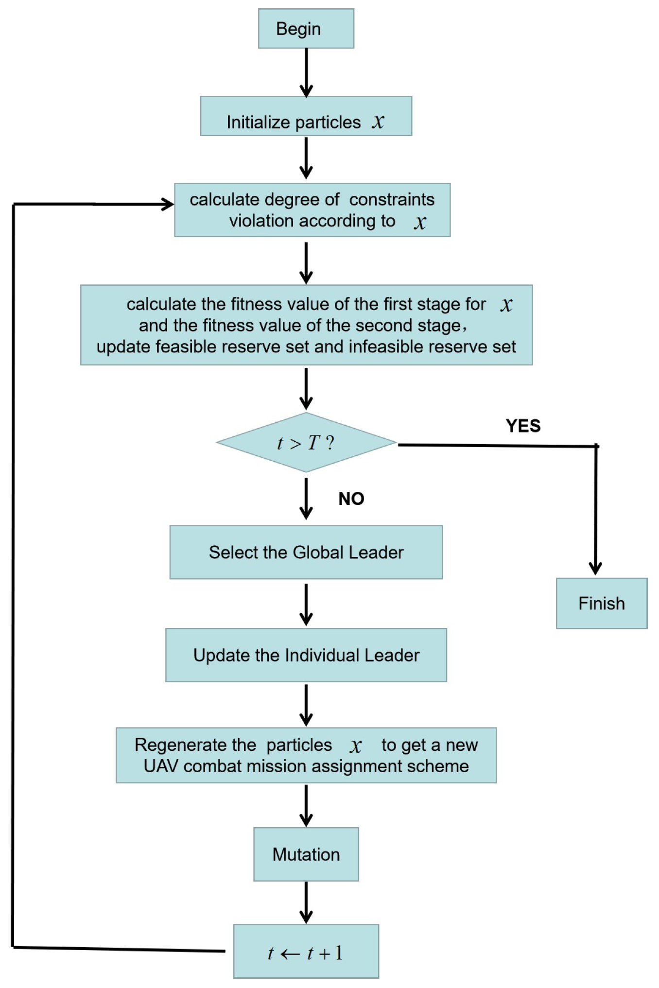
The algorithm flow chart is in Figure 1 as follows.

4. Improved PSO Algorithm

In Section 3, the problem is converted to the ETUCMA model which is solvable and deterministic. As the mathematical model established in this paper is a two-stage model, its algorithmic design is modified based on the fundamental principles of the basic particle swarm optimization (PSO) algorithm. This basic PSO algorithm includes initializing the particle swarm, computing particle fitness values, establishing initial individual and global best positions, updating these best positions, evolving the particle swarm, and enforcing boundary conditions. In the modified PSO, the individual leaders and global leaders can be found among particles that satisfy the constraints, as well as among particles that violate the constraints. Furthermore, the algorithm introduces novel strategies involving intersection and mutation to update particles, thereby preventing the algorithm from converging to local solutions and preserving population diversity. A comparative analysis was conducted between the results obtained from the original PSO algorithm and the improved PSO algorithm, in order to highlight the effectiveness of the improved PSO algorithm. In this part, a modified PSO algorithm is introduced.

4.1. Encoding

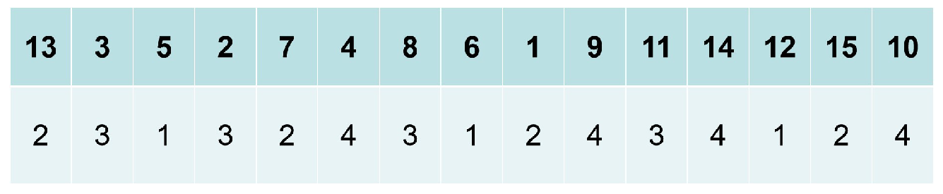
The encoding of the UAV combat mission assignment scheme is the most critical part of the algorithm. Traditional encoding cannot satisfy the requirements of the model due to the complexity of the objective function and constraint conditions; therefore, a new encoding method is introduced to overcome this problem. There are two rows for each particle: the top row contains targets from the set $\left\{T_1,T_2,\cdots ,T_m\right\}$, where m is denoted as the number of targets; the second row is the UAV chosen to attack target from the set $\left\{U_1,U_2,\cdots ,U_n\right\}$, where n is denoted as the number of UAVs. They are arranged according to the order of attacking target. Moreover, particles are split into a set of UAV-based sub-particles to visually indicate the order in which each UAV attacks targets. Figure 2 shows the encoding of the UAV combat mission assignment scheme. Figure 3 shows an example of a particle for the scenario of three targets being attacked by $U_1$,$(0\to 5\to 6\to 12)$, four targets being attacked by $U_3$, $(0\to 3\to 2\to 8\to 11)$, four targets being attacked by $U_2$, $(0\to 13\to 7\to 1\to 15)$, and four targets being attacked by $U_4$, $(0\to 4\to 9\to 14\to 10)$.

Remark 1.

Note that a sub-particle based on UAVs is a task sequence chain of a UAV; the particle is encoded based on all targets, so the constraints Equations (13)–(16) are naturally satisfied.

4.2. Design of Improved PSO Algorithm

Dealing with the two-stage model, a useful algorithm must be able to optimize UAV combat mission assignment schemes under various constraints. A modified particle swarm optimization (PSO) algorithm for solving the two-stage uncertain UAV combat mission assignment problem is proposed. Some concepts and the process of the algorithm are introduced as follows.

4.2.1. Constraint Violation

We introduce constraint violation to analyze the relations between the particle and the maximum flight distance constraints of the UAV. The particle x, that is, the UAV combat mission assignment scheme, is said to violate the constraint ${\mathit{D}}_k$$(k=1,2,\dots ,n)$ if $\mathit{x}$ does not satisfy one of the following conditions:

• (1) $dc{j}_1\left(\mathit{x}\right)={\displaystyle \sum _{j=1}^m\sum _{{\displaystyle \genfrac{}{}{0pt}{}{i\ne j\hfill }{i=0\hfill }}}^m}{d}_{(i,j)}{x}_{(i,j)}^1-D_1\le 0$;
• (2) $dc{j}_2\left(\mathit{x}\right)={\displaystyle \sum _{j=1}^m\sum _{{\displaystyle \genfrac{}{}{0pt}{}{i\ne j\hfill }{i=0\hfill }}}^m}{d}_{(i,j)}{x}_{(i,j)}^2-D_2\le 0$;
• …
• (n) $dc{j}_n\left(\mathit{x}\right)={\displaystyle \sum _{j=1}^m\sum _{{\displaystyle \genfrac{}{}{0pt}{}{i\ne j\hfill }{i=0\hfill }}}^m}{d}_{(i,j)}{x}_{(i,j)}^n-D_n\le 0$;

where $dcj\left(\mathit{x}\right)=(dc{j}_1,dc{j}_2,\dots ,dc{j}_n)$. $l\left(\mathit{x}\right)=(l_1\left(\mathit{x}\right),l_2\left(\mathit{x}\right),\dots ,l_n\left(\mathit{x}\right))$ is defined as the constraint violation degree of $\mathit{x}$. We have

$$\begin{array}{cc}\hfill dcjmax\left(\mathit{x}\right)& =\underset{k\in \{1,2,\dots ,n\}}{\max }dc{j}_k\left(\mathit{x}\right),dc{j}_{kdcjmax}\left(\mathit{x}\right)={\displaystyle \frac{dc{j}_k\left(\mathit{x}\right)}{dcjmax\left(\mathit{x}\right)}};\hfill \\ \hfill l_k\left(\mathit{x}\right)& =\max \{dc{j}_k\left(\mathit{x}\right),0\},k=1,2,\cdots ,n.\hfill \end{array}$$

(26)

4.2.2. Updating the Reserve Set

The reserve set of feasible particles is proposed, which is used to store better non-violation particles. The reserve set of infeasible particles is also proposed, which is used to store violation particles that are not so bad. And the global leader is selected from these two sets.

(a)

Updating the reserve set of feasible particles

The final reserve set of feasible particles is applied to provide a decision-making UAV combat mission assignment scheme. There are three steps to realize this purpose:

 Step 1:

$f_{new}=reserve\_feasible\cup feasible\_solution$.

 Step 2:

Calculating these fitness values of $f_{new}$ and sorting by values from smallest to largest. The fitness is the value of objective function, that is, the value of particle x in Equation (25).

 Step 3:

Selecting the few particles in $f_{new}$ with the minimum values in order and saving them in $reserve\_feasible$.

Whereas the reserve set of feasible particles is denoted by $reserve\_feasible$, the new feasible solution set is denoted by $feasible\_solution$, and $f_{new}$ denotes a new set.

(b)

Updating the reserve set of infeasible particles

There are two purposes in searching for the feasible particles from the set of infeasible particles that are infeasible assignment schemes: one is increasing the diversity of UAV combat mission assignment schemes; the second is exploring larger feasible areas by using the feasible particles close to the better feasible particles. The reserve set of infeasible particles can be renovated according to the following steps:

 Step 1:

$I_{new}=reserve\_infeasible\cup infeasible\_solution$.

 Step 2:

Calculating the fitness values of $I_{new}$ and sorting values from smallest to largest.

 Step 3:

Selecting the few particles in $I_{new}$ with the minimum values in order and saving them in $reserve\_infeasible$.

Whereas the reserve set of infeasible particles is denoted by $reserve\_infeasible$, the new infeasible solution set is denoted by $infeasible\_solution$, and $I_{new}$ denotes a new set.

4.2.3. Selecting the Global Leader

To select the global leader from $reserve\_feasible$ and $reserve\_infeasible$ with the probability $P\_rr$,

$$P\_rr=P\_r1-{\displaystyle \frac{time}{Tmax}}P\_r2;$$

(27)

where $time$ is the current number of iterations, and $Tmax$ is the iterations. $P\_r1$ and $P\_r2$ are real numbers satisfying $0\le P\_r2<P\_r1\le 1$. In the program simulation (Section 5), $P\_r1$ is set to 0.7, and $P\_r2$ is set to 0.6. From the strategy, it can be understood that in an earlier stage the global leader will be selected from the reserve set of unfeasible particles with a greater probability, so as to maintain the diversity of the assignment schemes, and selection gradually focuses on the reserve set of feasible particles in the later stage to deeply explore the better assignment schemes.

4.2.4. Regenerating the Particles

The new particles that are UAV combat mission assignment schemes are generated by intersection, individual leaders, and global leaders.

(a)

Intersection

$$omega={\displaystyle \frac{9}{10}}-{\displaystyle \frac{1}{2}}{\displaystyle \frac{time}{Tmax}};$$

(28)

where $omega$ is the inertia weight, and $rand$ denotes the random real number from 0 to 1.

If $rand<omega$, two different columns of each particle are randomly exchanged. The implemented method of the exchange is illustrated in Figure 4 as follows.

Otherwise, if $rand\ge omega$, the particle is left unchanged. Thus, $omega$ represents the tendency of the particle to maintain its previous velocity.

(b)

Generating under the guidance of global leaders

$c_1$ is the social coefficient. In the program simulation (Section 5), we found that setting $c_1$ to 0.7 yields better results. And, for specific problems, it can be tested and adjusted accordingly. If $rand\ge c_1$, some columns of the particle which is from the global leader are randomly picked, and the selected columns then replace the corresponding columns of the previous particle in order to generate a new particle. The implemented method of the replacement is illustrated in Figure 5 as follows.

(c)

Generating under the guidance of the individual leaders

$c_2$ is the cognitive coefficient. In the experimental simulations (Section 5), we found that setting $c_2$ to 0.7 yields better results. However, for specific problems, it can be tested and adjusted accordingly. If $rand\ge c_2$, some columns of the particle which is from the individual leader are randomly picked, and the selected columns then replace the corresponding columns of the previous particle in order to generate a new particle.

4.2.5. Mutation

Due to its rapid convergence, the algorithm may converge prematurely to local optima. To mitigate this limitation, the modified algorithm incorporates a mutation operator. The mutation probability $P\_m$ for the parameter X is calculated as follows:

$$P\_m=e^{-Xtime/\phantom{XtimeTmax}Tmax}.$$

(29)

The implemented method of the mutation can be described as follows:

Step 1:

Randomly generating a real number, $rand$, $0\le rand\le 1$.

Step 2:

If $rand<P\_m$, then randomly generating an integer, j, from 1 to m.

Step 3:

Replacing the UAV in row 2 of column j with another UAV from the set $\left\{U_1,U_2,\cdots ,U_n\right\}$ randomly.

Equation (29) indicates that the majority of assignment schemes are influenced by the mutation operator at the beginning, thereby enhancing global search capability. The effect of the mutation operator is weakened gradually with the increase in iterations, preventing the algorithm from prematurely converging to local optima.

4.2.6. Updating the Individual Leader

The particle with the minimum fitness value from the initial to current iteration time is named as the individual leader, which can be updated according to the new generated particles. Let $Indi\_leade{r}_i\left(time\right)$ be the individual leaders of the particles $x_i\left(time\right)$, $i=1,2,\dots ,M$, where M is the the number of particles in the population. The implemented method to update the individual leader is illustrated as follows:

Step 1:

If the fitness value of the new generated particle $x_i(time+1)$ is less than the fitness value of $Indi\_leade{r}_i\left(time\right)$, then $Indi\_leade{r}_i(time+1)=x_i(time+1)$.

Step 2:

Otherwise, $Indi\_leade{r}_i(time+1)=Indi\_leade{r}_i\left(time\right)$.

In conclusion, as shown in Figure 6, the framework of the modified PSO algorithm avoids local optima by generating new particles and introducing a mutation operator, balancing local exploitation and global exploration while maintaining the diversity of particles which are assignment schemes.

5. Examples

Through the analysis of the above sections of the model and algorithm, in this section we give some specific examples to verify the two-stage uncertain UAV combat mission assignment problem based on uncertainty theory.

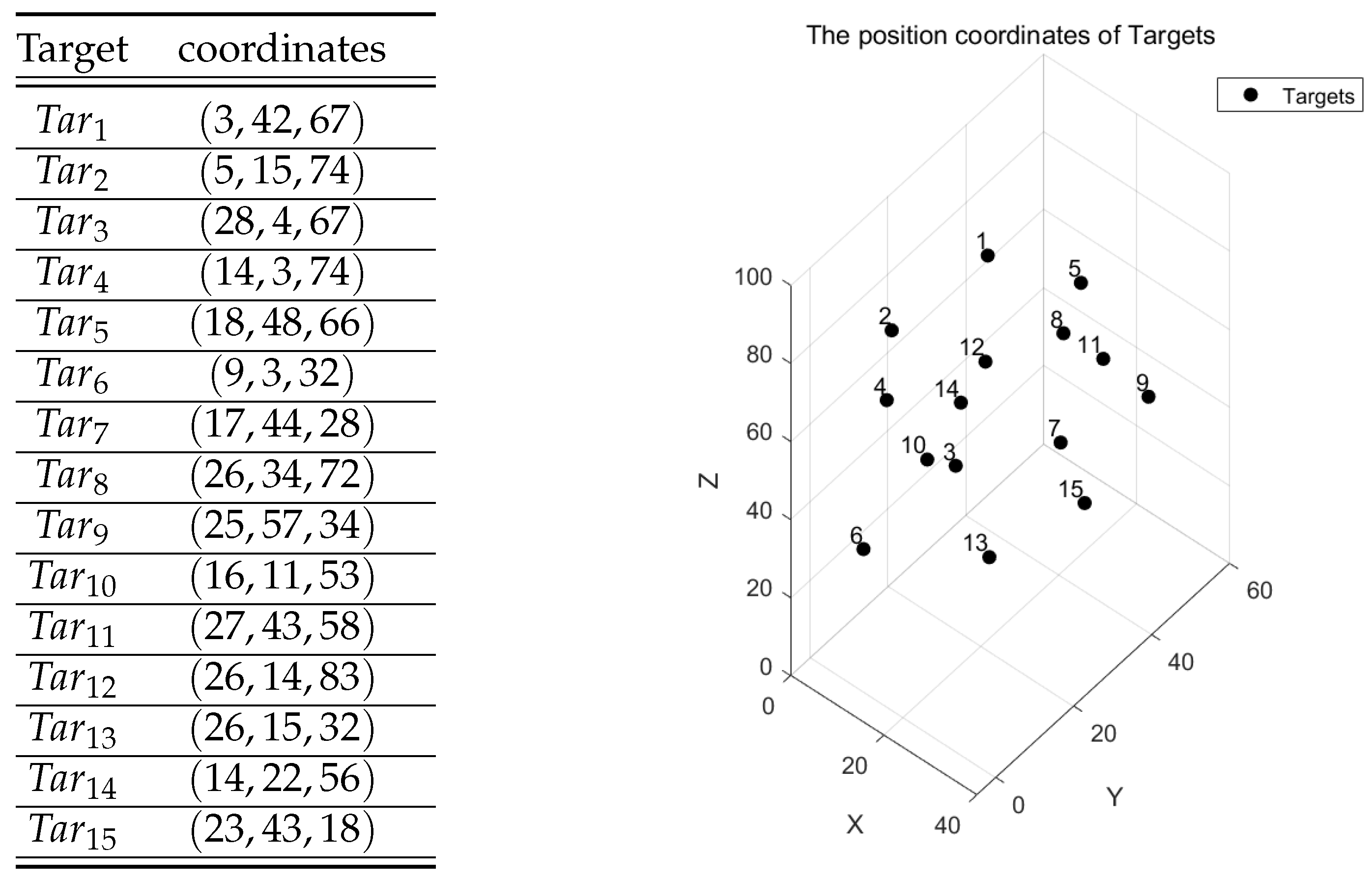
First, a combat scenario involving four UAVs and 15 task targets was constructed, with detailed specifications as follows. The value per unit of fuel, c, was set to 0.7. The maximum fuel storage $F_k$, the maximum flight distance $D_k$, the aircraft damage cost due to replenishing the fuel, $T_k$, and the zigzag uncertainty distribution ${\Phi }_{{\xi }_k}$ of the fuel consumption per unit of distance, ${\xi }_k$ ($k=1,2,3,4$), of UAVs are shown in

Table 1. Four UAVs’ information.

UAV	${\mathit{F}}_{\mathit{k}}$	${\mathit{D}}_{\mathit{k}}$	${\mathit{T}}_{\mathit{k}}$	${\mathbf{\Phi }}_{{\mathit{\xi }}_{\mathit{k}}}$
$U_1$	115.75	282	2.74	${\xi }_1$∼$Z(0.8,1.5,2)$
$U_2$	132.30	345.85	1.35	${\xi }_2$∼$Z(0.4,1,1.2)$
$U_3$	135.22	380.21	2.85	${\xi }_3$∼$Z(0.65,2,2.25)$
$U_4$	115.90	270	3.56	${\xi }_4$∼$Z(0.15,0.875,1.1875)$

.

The normal uncertainty distribution ${\Phi }_{{\eta }_j}$ of the target value ${\eta }_j$ ($j=1,2,\dots ,15$) is shown in

Table 2. Fifteen targets’ information.

Target	${\mathbf{\Phi }}_{{\mathit{\eta }}_{\mathit{j}}}$	Target	${\mathbf{\Phi }}_{{\mathit{\eta }}_{\mathit{j}}}$	Target	${\mathbf{\Phi }}_{{\mathit{\eta }}_{\mathit{j}}}$
$Ta{r}_1$	$\mathcal{N}\left(5,3.71\right)$	$Ta{r}_6$	$\mathcal{N}\left(4.3,2.7\right)$	$Ta{r}_{11}$	$\mathcal{N}\left(3.5,7.3\right)$
$Ta{r}_2$	$\mathcal{N}\left(9,3.8\right)$	$Ta{r}_7$	$\mathcal{N}\left(5.7,7.8\right)$	$Ta{r}_{12}$	$\mathcal{N}\left(2.09,2.1\right)$
$Ta{r}_3$	$\mathcal{N}\left(2.7,6.2\right)$	$Ta{r}_8$	$\mathcal{N}\left(8.2,5.1\right)$	$Ta{r}_{13}$	$\mathcal{N}\left(7.09,4.7\right)$
$Ta{r}_4$	$\mathcal{N}\left(3.4,6.3\right)$	$Ta{r}_9$	$\mathcal{N}\left(7.2,3.3\right)$	$Ta{r}_{14}$	$\mathcal{N}\left(6.04,2.8\right)$
$Ta{r}_5$	$\mathcal{N}\left(5.1,5.2\right)$	$Ta{r}_{10}$	$\mathcal{N}\left(4.8,6.7\right)$	$Ta{r}_{15}$	$\mathcal{N}\left(3.6,3.5\right)$

.

The coordinate positions of $Ta{r}_i$ (i-th target) ($i=1,2,\dots ,15$) are shown in Figure 7.

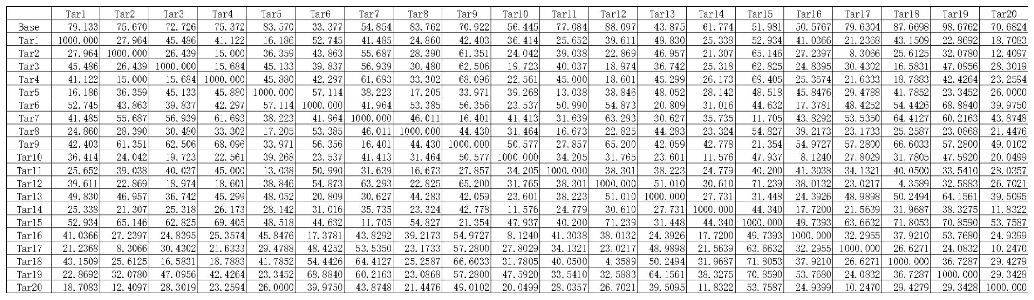
The distance $d(i,j)$ between $Ta{r}_i$ (i-th target) and $Ta{r}_j$ (j-th target) ($i,j=1,2,\dots ,15$) is shown in Figure 8.

The distance $d(i,i)$ between $Ta{r}_i$ and $Ta{r}_i$ was set to 1000 to avoid forming a loop that went from i to i ($i=1,2,\dots ,15$).

According to the analysis in Section 3.4, the two-stage uncertain UAV combat mission assignment problem can be constructed as follows:

$$\underset{x\in X_1}{min}{E}_{\xi }\left[\phi (x,\xi )\right]-{\int }_0^1(\sum _{k=1}^n\sum _{i=0}^m\sum _{{\displaystyle \genfrac{}{}{0pt}{}{j\ne i\hfill }{j=1\hfill }}}^m{\Phi }_{{\eta }_j}^{-1}\left(\alpha \right)x_{(i,j)}^k)d\alpha ;$$

where

$${\Phi }_{{\eta }_j}^{-1}\left(\alpha \right)=e_j+{\displaystyle \frac{{\sigma }_j\sqrt{3}}{\pi }}ln{\displaystyle \frac{\alpha }{1-\alpha }};{\Phi }_{{\eta }_j}=\mathcal{N}\left(e_j,{\sigma }_j\right);$$

$${\Phi }_{{\xi }_k}^{-1}\left(\alpha \right)=\left\{\begin{array}{cc}(2b_k-2a_k)\alpha +a_k,& \mathrm{if}\alpha <0.5;\\ (2c_k-2b_k)\alpha +2b_k-c_k,& \mathrm{if}\alpha \ge 0.5.\end{array};{\Phi }_{{\xi }_k}=Z(a_k,b_k,c_k).\right.$$

$E_{\xi }\left[\phi (x,\xi )\right]$ and $X_1$ were illustrated in Section 3.5. We solved the two-stage uncertain problem by the improved PSO algorithm and the original PSO algorithm via Matlab.

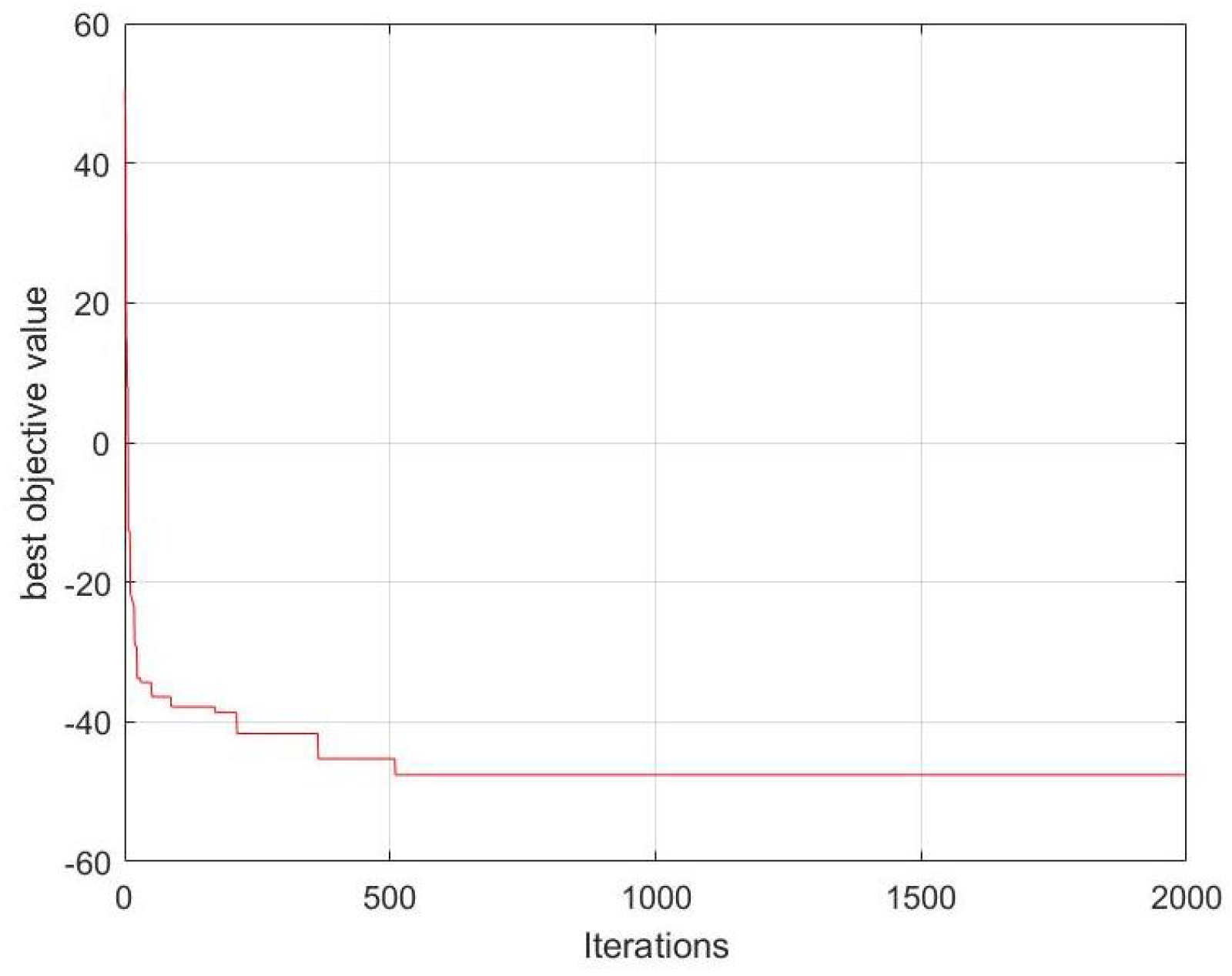
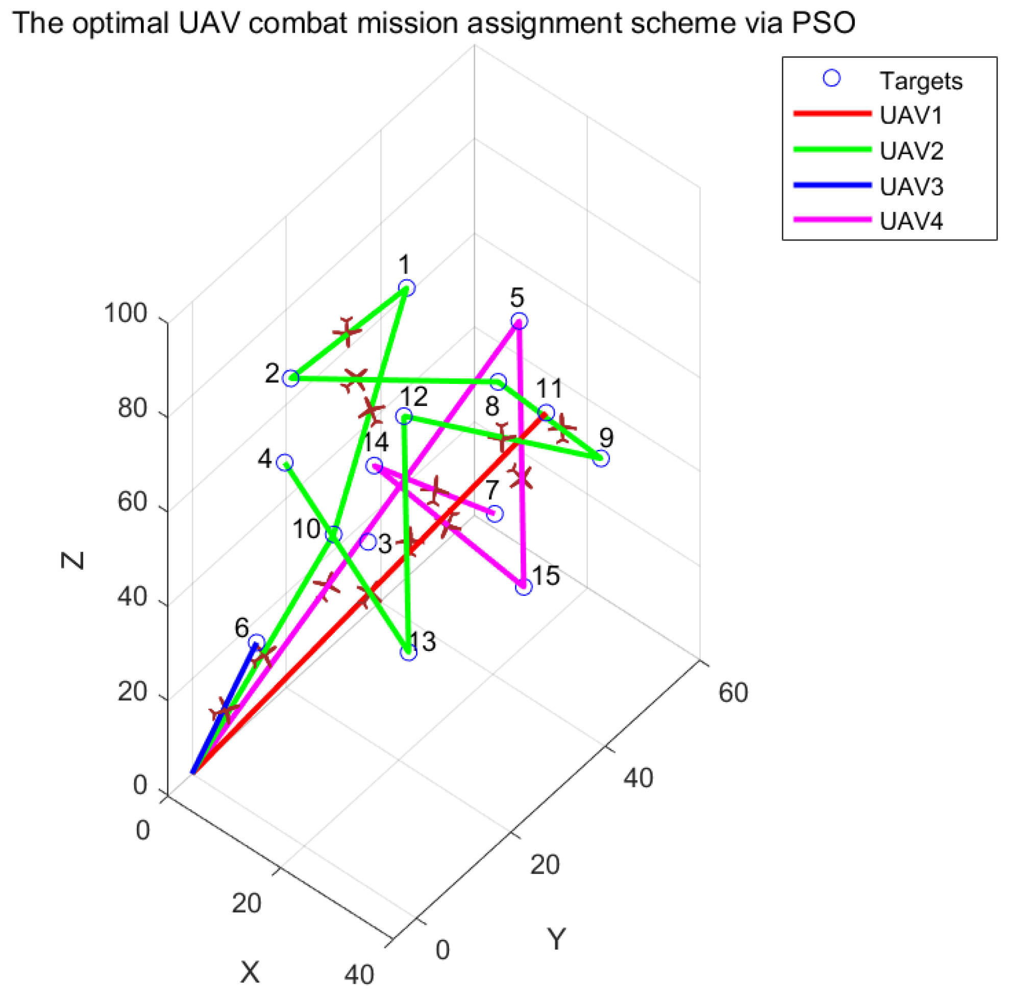
We set the maximum iteration limit to 2000. The results under the original PSO algorithm are presented in Figure 9. Convergence to a local optimum of 47.58 was achieved after the 510th iteration. Based on this, the UAV combat mission assignment scheme drone allocation is shown in

Table 3. The table of the optimal UAV combat mission assignment scheme obtained by PSO.

UAV	Task Trajectory
$U_1$	0→$Ta{r}_{11}$
$U_2$	0→$Ta{r}_{10}$→$Ta{r}_1$→$Ta{r}_2$→$Ta{r}_8$→$Ta{r}_9$→$Ta{r}_{12}$→$Ta{r}_{13}$→$Ta{r}_4$
$U_3$	0→$Ta{r}_6$
$U_4$	0→$Ta{r}_5$→$Ta{r}_{15}$→$Ta{r}_{14}$→$Ta{r}_7$

and in Figure 10, where it can be observed that Target 3 was not attacked.

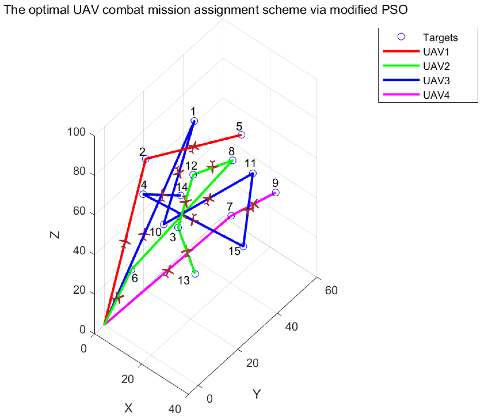
And under the improved PSO algorithm, the results are shown in Figure 11. We present the optimal UAV combat mission assignment scheme in

Table 4. The optimal UAV combat mission assignment table obtained by modified PSO.

UAV	Task Trajectory
$U_1$	0→$Ta{r}_2$→$Ta{r}_5$
$U_2$	0→$Ta{r}_6$→$Ta{r}_8$→$Ta{r}_{12}$→$Ta{r}_3$→$Ta{r}_{13}$
$U_3$	0→$Ta{r}_1$→$Ta{r}_{10}$→$Ta{r}_{11}$→$Ta{r}_{15}$→$Ta{r}_4$→$Ta{r}_{14}$
$U_4$	0→$Ta{r}_7$→$Ta{r}_9$

and in Figure 12. From Figure 12, we can see that all targets attacked by the all UAVs satisfied constraints. Further, it can be noticed that targets were attacked by different UAVs. Moreover, the results show that the objective value was −86.55; that is, the maximum target values was 86.55. We set the maximum iteration limit to 1000, and it quickly converged to the optimal solution after only 69 iterations. This indicates that the modified PSO algorithm was more effective.

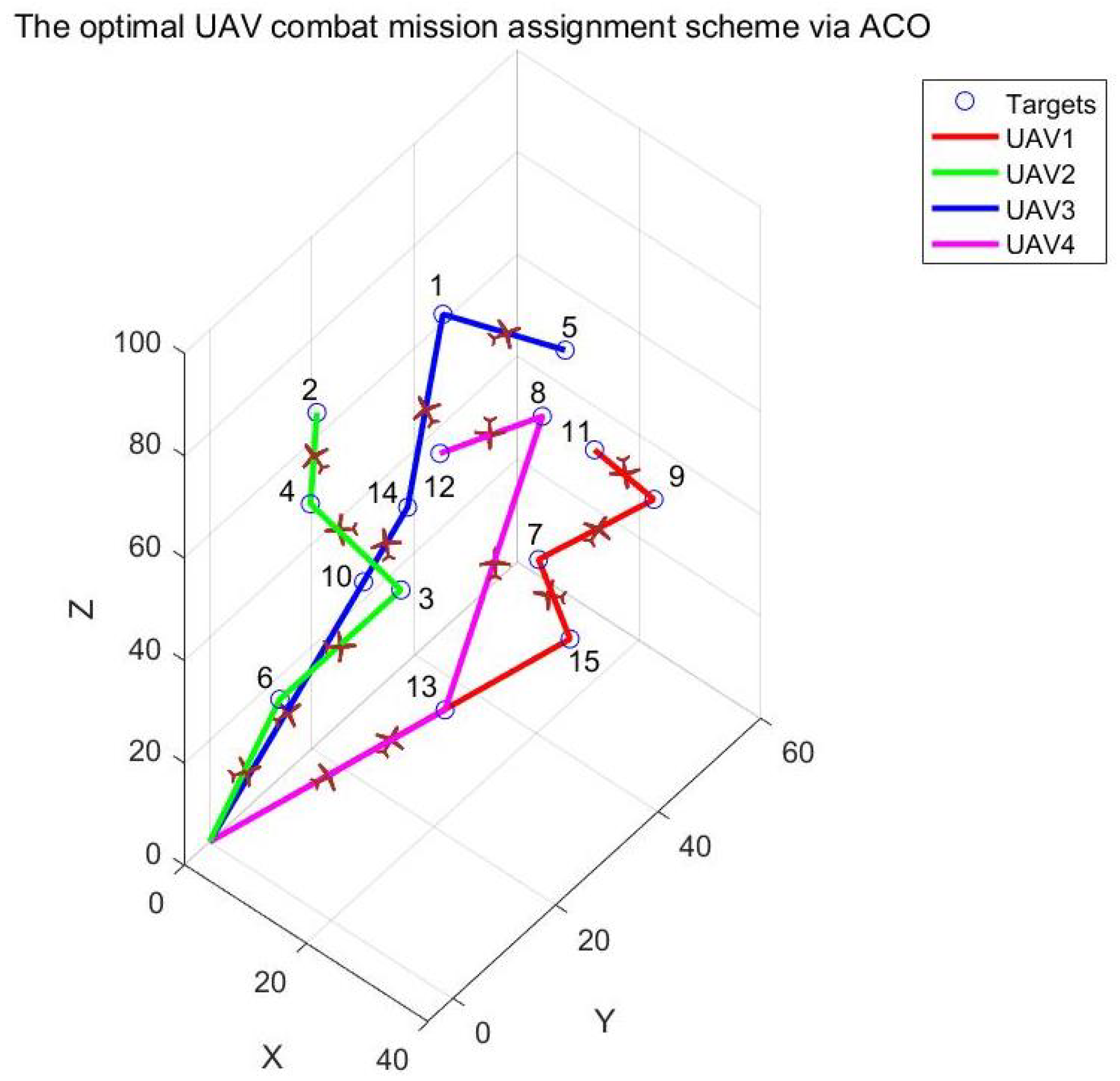
To further validate the effectiveness of the the modified PSO algorithm, we conducted simulation comparisons with ant colony optimization (ACO). Under identical parameter settings—where four UAVs engaged 15 targets—the result is shown in Figure 13. We also present the optimal UAV combat mission assignment scheme in

Table 5. The table of the optimal UAV combat mission assignment scheme obtained by ACO.

UAV	Task Trajectory
$U_1$	0→$Ta{r}_{15}$→$Ta{r}_7$→$Ta{r}_9$→$Ta{r}_{11}$
$U_2$	0→$Ta{r}_6$→$Ta{r}_3$→$Ta{r}_4$→$Ta{r}_2$
$U_3$	0→$Ta{r}_{10}$→$Ta{r}_{14}$→$Ta{r}_1$→$Ta{r}_5$
$U_4$	0→$Ta{r}_{13}$→$Ta{r}_8$→$Ta{r}_{12}$

and in Figure 14. From Figure 14, we can see that the ACO rapidly converged to a local optimum value of 36.31, demonstrating its susceptibility to premature convergence. This highlights the limitation of ACO in escaping local optimal solutions due to its heuristic pheromone-based search strategy, which often leads to the myopic exploration of the solution space.

In contrast, the modified PSO significantly enhances its global search capability through strategies such as dynamic inertia weight adjustment and mutation. Under identical experimental conditions, the modified PSO successfully escaped local optima and achieved a superior target values 86.55, verifying its effectiveness in avoiding premature convergence and approximating global optimal solutions. The results demonstrate that the modified PSO significantly outperforms the traditional ACO in both solution quality and robustness for the two-stage uncertain UAV combat mission assignment problem.

Next, we constructed a more complex combat scenario, where six UAVs were tasked with striking 20 mission targets. The specific details are as follows. The value per unit fuel c was also set to 0.7. The maximum fuel storage $F_k$, the maximum flight distance $D_k$, the aircraft damage cost due to replenishing the fuel $T_k$, and the zigzag uncertainty distribution ${\Phi }_{{\xi }_k}$ of the fuel consumption per unit distance, ${\xi }_k$ ($k=1,2,3,4,5,6$), of UAVs are shown in

Table 6. Six UAVs’ information.

UAV	${\mathit{F}}_{\mathit{k}}$	${\mathit{D}}_{\mathit{k}}$	${\mathit{T}}_{\mathit{k}}$	${\mathbf{\Phi }}_{{\mathit{\xi }}_{\mathit{k}}}$
$U_1$	115.75	282	2.74	${\xi }_1$∼$Z(0.8,1.5,2)$
$U_2$	132.30	345.85	1.35	${\xi }_2$∼$Z(0.4,1,1.2)$
$U_3$	135.22	380.21	2.85	${\xi }_3$∼$Z(0.65,2,2.25)$
$U_4$	115.90	270	3.56	${\xi }_4$∼$Z(0.15,0.875,1.1875)$
$U_5$	121.11	379.07	2.7	${\xi }_5$∼$Z(0.34,0.9,1.1)$
$U_6$	125.7	250.05	1.8	${\xi }_6$∼$Z(0.18,0.3,0.5)$

.

The normal uncertainty distribution ${\Phi }_{{\eta }_j}$ of the target value ${\eta }_j$ ($j=1,2,\dots ,20$) is shown in

Table 7. Twenty targets’ information.

Target	${\mathbf{\Phi }}_{{\mathit{\eta }}_{\mathit{j}}}$	Target	${\mathbf{\Phi }}_{{\mathit{\eta }}_{\mathit{j}}}$	Target	${\mathbf{\Phi }}_{{\mathit{\eta }}_{\mathit{j}}}$	Target	${\mathbf{\Phi }}_{{\mathit{\eta }}_{\mathit{j}}}$
$Ta{r}_1$	$\mathcal{N}\left(5,3.71\right)$	$Ta{r}_6$	$\mathcal{N}\left(4.3,2.7\right)$	$Ta{r}_{11}$	$\mathcal{N}\left(3.5,7.3\right)$	$Ta{r}_{16}$	$\mathcal{N}\left(7.1,8.4\right)$
$Ta{r}_2$	$\mathcal{N}\left(9,3.8\right)$	$Ta{r}_7$	$\mathcal{N}\left(5.7,7.8\right)$	$Ta{r}_{12}$	$\mathcal{N}\left(2.09,2.1\right)$	$Ta{r}_{17}$	$\mathcal{N}\left(6.7,3.5\right)$
$Ta{r}_3$	$\mathcal{N}\left(2.7,6.2\right)$	$Ta{r}_8$	$\mathcal{N}\left(8.2,5.1\right)$	$Ta{r}_{13}$	$\mathcal{N}\left(7.09,4.7\right)$	$Ta{r}_{18}$	$\mathcal{N}\left(4.4,2.7\right)$
$Ta{r}_4$	$\mathcal{N}\left(3.4,6.3\right)$	$Ta{r}_9$	$\mathcal{N}\left(7.2,3.3\right)$	$Ta{r}_{14}$	$\mathcal{N}\left(6.04,2.8\right)$	$Ta{r}_{19}$	$\mathcal{N}\left(3.5,5.6\right)$
$Ta{r}_5$	$\mathcal{N}\left(5.1,5.2\right)$	$Ta{r}_{10}$	$\mathcal{N}\left(4.8,6.7\right)$	$Ta{r}_{15}$	$\mathcal{N}\left(3.6,3.5\right)$	$Ta{r}_{20}$	$\mathcal{N}\left(8.1,6.5\right)$

.

The coordinate positions of the $Ta{r}_i$ (i-th target) ($i=1,2,\dots ,20$) are shown in Figure 15.

The distance $d(i,j)$ between $Ta{r}_i$ (i-th target) and $Ta{r}_j$ (j-th target) ($i,j=1,2,\dots ,20$) is shown in Figure 16.

The results under the modified PSO algorithm are shown in Figure 17. We present the optimal UAV combat mission assignment scheme in

Table 8. The optimal UAV combat mission assignment table for 20 Targets and 6 UAVs obtained by modified PSO.

UAV	Task Trajectory
$U_1$	0→$Ta{r}_{15}$
$U_2$	0→$Ta{r}_6$→$Ta{r}_{13}$→$Ta{r}_{14}$
$U_3$	0→$Ta{r}_{10}$
$U_4$	0→$Ta{r}_{16}$→$Ta{r}_{20}$ →$Ta{r}_2$→$Ta{r}_{17}$
$U_5$	0→$Ta{r}_3$→$Ta{r}_4$→$Ta{r}_{12}$
$U_6$	0→$Ta{r}_9$→$Ta{r}_7$ →$Ta{r}_1$→$Ta{r}_5$ →$Ta{r}_{11}$ →$Ta{r}_8$→$Ta{r}_{19}$→$Ta{r}_{18}$

and in Figure 18. From Figure 18, it can be observed that all targets were successfully engaged by the all UAVs. Furthermore, the results show that the maximum target values achieved was 107.52. With the maximum iteration limit also set to 1000, and the algorithm quickly converged to the optimal solution after only 122 iterations. That indicates that the modified PSO algorithm demonstrates strong applicability to complex task mission assignment scenarios, highlighting its robust practical utility in real-world task allocation problems.

Finally, the simulation results of the above examples demonstrate that the modified PSO algorithm proposed in this paper is highly effective. It not only achieves superior performance in combat mission assignment efficiency but also shows strong adaptability to complex scenarios, significantly outperforming conventional methods. These results fully validate the practicality, reliability, and outstanding the advantages of the proposed modified PSO algorithm. In summary, the two-stage uncertain model and the modified PSO algorithm proposed in this paper demonstrate applicability to UAV combat scenarios, enabling the derivation of an optimal task allocation scheme that maximizes target values.

6. Conclusions

In this paper, we discuss the UAV combat mission assignment problem. Due to the complex and changeable environment of the battlefield, the unit fuel consumption of UAVs and the target value are both uncertain factors and we established a two-stage uncertain UAV combat mission assignment model. There is no large amount of sample data to obtain a probability distribution, so we cannot expect to use a mature knowledge system such as probability theory and mathematical statistics to solve the uncertain problem in such uncertain environment. Therefore, this paper is based on the new axiomatic mathematical system named uncertainty theory; UAV unit fuel consumption and mission target values are uncertain variables, corresponding to the uncertainty distributions. First, a two-stage uncertain UAV combat mission assignment (TUCMA) model was established. And we transformed the TUCMA model to the solvable deterministic ETUCMA model. Then, as the model is a two-stage model, a modified PSO algorithm based on the fundamental principles of the basic particle swarm optimization (PSO) algorithm was designed. Finally, examples were applied to obtain the optimal allocation scheme. And the number of iterations was 1000; the optimal value was obtained in the 69-th iteration, indicating that the proposed model and algorithm are effective. In our study, we compared the modified PSO algorithm with the original particle swarm optimization algorithm and the ant colony optimization algorithm. In Section 5, with examples provided, we presented comparisons of the results of the algorithms. The results clearly demonstrate that the modified PSO algorithm exhibits superior convergence properties, capable of achieving global optimality. In contrast, the original particle swarm algorithm often tends to get stuck in local optima, primarily due to the absence of mutation operations, which significantly reduces the diversity of solutions; the ant colony optimization algorithm often leads to the myopic exploration of the solution space due to its heuristic pheromone-based search strategy. This lack of diversity limits the algorithm’s ability to explore the solution space, making it difficult to find the global optimum.

However, real combat problems are more complex, including factors such as altitude limitations on UAV flight, changes in environmental terrain, wind speed, and so on. In follow-up, we can use the model in this article as a basis and consider more uncertain factors to construct a more realistic model, and we can also apply the two-stage model to other military issues. In conclusion, the issues discussed in this paper are of far-reaching significance. There is a lot of knowledge to be discovered and studied in depth, and the application potential is strong.

References

Alqudsi, Y.; Makaraci, M. UAV swarms: Research, challenges, and future directions. J. Eng. Appl. Sci.2025, 72, 12. [Google Scholar] [CrossRef]
Chen, L.; Liu, W.L.; Zhong, J. An Efficient Multi-Objective Ant Colony Optimization for Task Allocation of Heterogeneous Unmanned Aerial Vehicles. J. Comput. Sci.2022, 58, 101545. [Google Scholar] [CrossRef]
Yue, W.; Zhang, X.; Liu, Z. Distributed Cooperative Task Allocation for Heterogeneous UAV Swarms under Complex Constraints. Comput. Commun.2025, 231, 108043. [Google Scholar] [CrossRef]
Vohra, D.; Garg, P.; Ghosh, S. Usage of UAVs/drones based on their aategorisation: A review. J. Aerosp. Sci. Technol.2023, 74, 90–101. [Google Scholar]
Qadir, Z.; Ullah, F.; Munawar, H.S.; Al-Turjman, F. Addressing disasters in smart cities through UAVs path planning and 5G communications: A systematic review. Comput. Commun.2021, 168, 114–135. [Google Scholar] [CrossRef]
Dantzig, G.B. Linear programming under uncertainty. Manag. Sci.1955, 3–4, 197–206. [Google Scholar] [CrossRef]
Front Matter. In Lectures on Stochastic Programming: Modeling and Theory, 3rd ed.; Society for Industrial and Applied Mathematics (SIAM): Philadelphia, PA, USA, 2021; pp. i–xv.
Jordehi, A.R.; Tabar, V.S.; Mansouri, S.A.; Sheidaei, F.; Ahmarinejad, A.; Pirouzi, S. Two-stage stochastic programming for scheduling microgrids with high wind penetration including fast demand response providers and fast-start generators. Sustain. Energy Grids Netw.2022, 31, 100694. [Google Scholar] [CrossRef]
Pasupathy, R.; Song, Y. Adaptive sequential sample average approximation for solving two-stage stochastic linear programs. SIam J. Optim.2021, 31, 1017–1048. [Google Scholar] [CrossRef]
Irawan, C.A.; Hofman, P.S.; Chan, H.K.; Paulraj, A. A stochastic programming model for an energy planning problem: Formulation, solution method and application. Ann. Oper. Res.2022, 311, 695–730. [Google Scholar] [CrossRef]
Ramaraj, G.; Hu, Z.; Hu, G. A two-stage stochastic programming model for production lot-sizing and scheduling under demand and raw material quality uncertainties. Int. J. Plan. Sched.2019, 3, 1. [Google Scholar] [CrossRef]
Basciftci, B.; Ahmed, S.; Gebraeel, N. Adaptive two-stage stochastic programming with an analysis on capacity expansion planning problem. arXiv2024, arXiv:1906.03513. [Google Scholar] [CrossRef]
MacNeil, M.; Bodur, M. Leveraging decision diagrams to solve two-stage stochastic programs with binary recourse and logical linking constraints. Eur. J. Oper. Res.2024, 315, 228–241. [Google Scholar] [CrossRef]
Alqefari, S.; Menai, M.E.B. Multi-UAV task assignment in dynamic environments: Current trends and future directions. Drones2025, 9, 75. [Google Scholar] [CrossRef]
Liu, B. Uncertainty Theory: A Branch of Mathematics for Modeling Human Uncertainty; Springer: Berlin/Heidelberg, Germany, 2010; Volume 300. [Google Scholar]
Jia, Y.; Lio, W. Tightness of triangle inequality in uncertainty theory. Soft Comput.2023, 27, 14621–14630. [Google Scholar] [CrossRef]
Zeng, Z.; Kang, R.; Wen, M.; Zio, E. Uncertainty theory as a basis for belief reliability. Inf. Sci.2017, 429. [Google Scholar] [CrossRef]
Funfschilling, C.; Perrin, G. Uncertainty quantification in vehicle dynamics. Veh. Syst. Dyn.2019, 57, 1062–1086. [Google Scholar] [CrossRef]
Li, B.; Zhang, R.; Sun, Y. Multi-period portfolio selection based on uncertainty theory with bankruptcy control and liquidity. Automatica2023, 147, 110751. [Google Scholar] [CrossRef]
Lio, W.; Kang, R. Bayesian rule in the framework of uncertainty theory. Fuzzy Optim. Decis. Mak.2022, 22, 337–358. [Google Scholar] [CrossRef]
Zhang, B.; Sang, Z.; Xue, Y.; Guan, H. Research on optimization of customized bus routes based on uncertainty theory. J. Adv. Transp.2021, 2021, 6691299. [Google Scholar] [CrossRef]
Figure 1.
Algorithm flow chart.
Figure 2.
Encoding the particle.
Figure 3.
Encoding the sub-particle.