Uncertainty Modeling of Fouling Thickness and Morphology on Compressor Blade

Abstract

To describe the fouling characteristics of compressor blades, fouling is categorized into dense and loose layers to characterize thickness and rough structures. An uncertainty model for dense fouling layer thickness distribution is constructed using the numerical integration and the Karhunen–Loève (KL) expansion method, while the Fouling Longuet-Higgins (FLH) model is proposed to address the uncertainty of loose fouling layer roughness. The FLH model effectively simulates the morphology characteristics of actual blade fouling and elucidates how parameters influence fouling roughness, morphology, and randomness. Based on the uncertainty modeling method, models for dense fouling layer thickness and loose fouling layer morphology are constructed, followed by numerical calculations and aerodynamic performance uncertainty quantification. Results indicate a 75.8% probability of aerodynamic performance degradation due to a dense fouling layer and a 97.2% probability related to the morphology uncertainty of a loose fouling layer when the roughness is 50 μm. This underscores that a mere focus on roughness is inadequate for characterizing blade fouling, and a comprehensive evaluation must also incorporate the implications of rough structures on aerodynamic performance.

1. Introduction

The compressor is the core component of the aero engine. The fouling of compressor blades formed by air pollution is considered to be the most important factor causing service performance degradation and potential safety risks of modern aero engines [1,2,3]. Consequently, accurately characterizing blade fouling and the quantitative assessment of their effects on aerodynamic performance have become important subjects of current research.

Over the years, investigations have been conducted into the deposition issues related to fouling on compressor blades [4,5,6]. Studies have demonstrated that airborne dust, inherent suspended particulate matter, saline mist in coastal areas, and environmental factors such as air temperature and humidity all influence the deposition of fouling on compressor blades [7,8,9,10,11]. The complex topography and variable environment lead to a diverse composition and intricate morphology of dust particles, as well as a broad particle size distribution, which results in significant uncertainty regarding the distribution and morphology of fouling on compressor blades.

The fouling distribution and morphology of the blade surface are usually obtained by actual measurement and two-phase flow deposition simulation. It has been widely noted in fouling distribution and morphology studies that the roughness and location of the distribution of fouling are of interest. Taylor measured the surface roughness of 30 blades from the first stages of operational engines, namely the F-100 (fighter jet) and TF-39 (transport aircraft), and found that the TF-39 blades were roughest on the pressure side near the mid-chord and trailing edge, while the F-100 blades exhibited maximum roughness on the suction side near the leading edge, with maximum roughness heights reaching 50 μm and 79 μm, respectively [12]. Mullaney [13] scanned the surface fouling morphology of actual aerospace compressor blades and found that the surface fouling morphology of different blades and cross-sections is completely different. Furthermore, research conducted by Cranfield University [14], the Norwegian University of Science and Technology [15], the University of Stuttgart [1], and the University of Ferrara [5,16,17] indicated that there are no discernible patterns in the deposition of particles on the blade surfaces.

However, some studies have analyzed fouling utilizing electron microscope scanning and found not only different rough structure features on the fouling surface but also a dense layer of particles, that is the thickness of the fouling, forming first near the wall [18,19,20]. Similarly, the thickness of fouling is necessarily non-uniform and characterized by uncertainty affected by a variety of factors. In addition, the thickness of fouling varies under the influence of factors such as flight time and weather, and this variation is the main source of its uncertainty.

For many years, researchers both domestically and internationally have conducted a series of experiments and numerical studies by simplifying fouling into a form of thickness and roughness. In experimental studies, researchers have characterized the fouling morphology by applying coatings to the blade surfaces [21], attaching sandpaper [22,23], or spraying paint or adhesive [14,24]. In numerical studies, researchers [25,26,27,28,29,30] commonly adopt thickened blades combined with equivalent gravel models that simulate surface roughness. Research results on the aerodynamic performance degradation of fouled compressor blades indicate that fouling leads to a decline in overall performance, with a significant impact from fouling roughness on the leading edge and the front half of the suction surface on compressor performance degradation.

Unfortunately, the above studies on fouling thickness have mainly used uniform thickness to characterize it, ignoring the influence of non-uniform fouling on the degradation of aerodynamic performance. Meanwhile, it is worth noting that the equivalent gravel model approximates rough surfaces as uniform spherical particles and is used to study the effect of rough surfaces on aerodynamic performance [31]. While this approach provides some insight into the effects of fouling on aerodynamic performance degradation, it tends to reduce these effects to a single geometric parameter—roughness—thereby overlooking the irregular distribution and complex rough structures of fouling on actual compressor blade surfaces, which are influenced by factors such as airflow, particle size, and physical properties [12,32,33,34,35,36,37]. Research indicates that when the roughness deviates from a spherical gravel configuration, a single parameter is no longer sufficient to characterize the roughness accurately [34].

Recently, advanced data-driven and machine learning (ML) approaches have shown significant promise in predicting compressor blade fouling. Researchers have increasingly leveraged techniques such as computer vision for automatic recognition of fouling morphological features from scanned blade surface images [38,39], physics-informed neural networks (PINNs) for simulating complex gas–solid two-phase deposition processes [40], and supervised learning models trained on extensive operational data to forecast fouling severity and its performance impacts [41,42]. These methods demonstrate powerful capabilities in handling high-dimensional, non-linear problems and uncovering complex patterns from data. Notwithstanding these advances, data-driven approaches often require substantial volumes of high-quality, scenario-specific training data. Their predictive models can sometimes lack strong physical interpretability, and they face challenges in explicitly characterizing the inherent physical randomness and quantifying the uncertainties associated with the non-uniform distribution of fouling thickness and the stochastic nature of rough surface structures. More importantly, in the existing studies, there is almost no relevant research on the modeling method of geometric uncertainty of fouling compressor blades and the degradation of their aerodynamic performance.

Consequently, the small size and high loading of compressor blades result in their extreme sensitivity to aerodynamic performance, and previous studies that simplified the fouling thickness to a uniform variation will not accurately obtain the law of influence of real blade fouling on aerodynamic performance. The equivalent gravel model shows certain limitations in capturing the irregular roughness features of fouled compressor blades, thereby impeding a more profound understanding and precise prediction of fouling phenomena. In light of these considerations, it is essential to fully account for the uncertainties in the thickness distribution and rough structures of fouling on compressor blades in this study, establish the uncertainty model for blade fouling, and investigate its effects on aerodynamic performance degradation. This study proposes a novel fouling uncertainty methodology, departing from conventional research focused on specific fouling morphologies. It represents an innovative contribution to blade fouling modeling and fouling effect prediction.

To quantitatively characterize the non-uniformity of fouling thickness distribution and the randomness of rough structures, this study proposes an uncertainty modeling method for compressor blade fouling. Based on fouling characteristics, the model separately constructs dense layer fouling thickness and loose layer fouling roughness: The dense layer distribution describes the non-uniformity and uncertainty of fouling thickness, while the loose layer characterizes roughness parameters including surface roughness, wavelength characteristics, and skewness of fouling structures. The characterization capability of the loose layer fouling model is validated using actual scanned fouling morphologies. By coupling the developed fouling modeling approach with uncertainty quantification methods, a quantitative model is established to correlate fouling uncertainties with aerodynamic performance responses. Finally, the feasibility of both the fouling modeling methodology and aerodynamic performance uncertainty quantification approach is verified through comprehensive validation considering fouling distribution non-uniformity and roughness structure randomness.

This study proposes an uncertainty modeling method for compressor blade fouling. The main structure of the paper is as follows: Part 1 discusses the significance of fouling uncertainty research and the necessity of developing uncertainty modeling methods. Part 2 introduces fouling characteristics and the uncertainty modeling approach, validating its accuracy using actual blade surface fouling morphology data. Part 3 employs a representative diffuser cascade to verify the feasibility of the modeling method and present predictions of aerodynamic performance degradation.

2. Fouling Uncertainty Modeling Method

2.1. Description of Fouling Morphology

Based on the scanning image of the surface morphology of the particle deposition on the flat plate [26], it can be noticed that the fouling increases the non-uniform thickness of the flat plate and the irregular surface roughness. To characterize the fouling, some spherical particles with random diameters are used to describe the distribution and morphology of the flat plate fouling as shown in Figure 1. In general, with the accumulation of time and the pressure of the airflow during the deposition of particles, a relatively dense fouling layer must be formed near the wall first. With the increase in time, the thickness of the dense layer gradually increases, and there is always a relatively loose particle layer in the outermost layer. Therefore, the fouling is classified into a dense layer and a loose layer by sufficiently considering the fouling distribution characteristics in the normal direction of the flat plate, which represent the non-uniform thickness and rough structures of the fouling, respectively. Therefore, fouling can be calculated by the following equation:

$$H\left(x\right)=h_1\left(x\right)+h_2\left(x\right)$$

(1)

where x stands for the coordinates, h₁(x) represents dense fouling layer, and h₂(x) represents loose fouling layer.

The fouling on the surface of a compressor blade is similar to flat plate fouling in that it is the deposition of particles over some time, which is also manifested in the variation in the thickness of the fouling and the irregular surface roughness, that is, the dense fouling layer and the loose fouling layer. However, compressor blade fouling is affected by many factors such as operating conditions and uncertainty.

Considering the uncertainty of fouling formation conditions, the complex shape of the blades and the frequent flights under variable operating conditions mainly lead to the uncertainty of the thickness of the dense fouling layer, while the diversity of particle sizes and shapes mainly leads to the uncertainty of the rough structures of the loose fouling layer. Therefore, Formula (2) is used to describe the uncertainty in the thickness of the dense fouling layer and the rough structures of the loose fouling layer of the compressor blade.

$$H\left(x,\theta \right)=h_1\left(x,\theta \right)+h_2\left(x,\theta \right)$$

(2)

Here, a random space θ is introduced to describe the uncertainty of the fouling.

2.2. Uncertainty Modeling Method of Dense Fouling Layer Thickness

A critical aspect of studying the uncertainty in the morphology and distribution of fouling on compressor blades is modeling the geometrical uncertainty associated with this fouling. The uncertainty of fouling thickness is reflected in the different thicknesses of fouling at the same location and the different thicknesses of fouling at different locations. For this study, the uncertainty in the thickness of fouling at the same location is described by the mean ($\overline{h_1}$) and disturbance value ($h_1^{\prime }$), and the position variable (control point position) x is used to describe the variation in fouling thickness with position. Therefore, the thickness of the dense fouling layer h₁ can be calculated using the following formula:

$$h_1\left(x,\theta \right)=\overline{h_1\left(x\right)}+h_1^{\prime }\left(x,\theta \right)$$

(3)

It is worth noting that the mean value ($\overline{h_1}$) of the dense fouling layer thickness is a statistic obtained from a large number of measurements, while the perturbation value is calculated from the mean ($\overline{h_1}$) and standard deviation (${\sigma }_{h_1}$) of the dense fouling layer thickness.

To model the uncertainty in the thickness of the dense fouling layer, it is fundamental to calculate the disturbance values of the thickness of the dense fouling layer, in particular, the number of control point positions x determines the dimension of the modeling. Among them, the position diagram of the control point is shown in Figure 2. The positions of the control points on the blade arc are marked with short lines, and the leading edge is written as LE, suction surface is marked as SS, trailing edge is marked as TE, and the pressure surface is marked as PS. For this study, the blade arc is separated from the trailing edge point along the arc and the position of each control point is normalized in the direction of the trailing edge, suction surface, leading edge, and pressure surface. And s is the total length of the blade arc.

Based on the mean $\overline{h_1\left(x\right)}$ and standard deviation ${\sigma }_{h_1}\left(x\right)$ of the corresponding control point locations, the KL expansion method is employed to construct the uncertain non-uniform dense fouling layer of a compressor blade, which is calculated as follows:

$$h_1^{\prime }\left(x,\theta \right)\approx {\displaystyle {\sum }_{i=1}^M}\sqrt{{\lambda }_i}{\phi }_i\left(x\right){\xi }_i\left(\theta \right)$$

(4)

where λ_i is the ith eigenvalue of the covariance matrix C_cov constructed from the mean $\overline{h_1\left(x\right)}$ and standard deviation ${\sigma }_{h_1}\left(x\right)$ of the thickness of the dense fouling layer, φ_i(x) is the eigenvector corresponding to the ith eigenvalue of the covariance matrix C_cov, ${\xi }_i\left(\theta \right)$ is an independent and equally distributed random variable satisfying a standard Gaussian distribution, and M is the number of eigenvalues and eigenvectors required for constructing the non-uniform dense fouling layer thickness of a compressor blade, and the computation formula is

$${\displaystyle \frac{{\displaystyle {\sum }_{i=1}^M}{\lambda }_i}{{\displaystyle {\sum }_{i=1}^N}{\lambda }_i}}⩾p\%$$

(5)

Here, N is the number of control points, and p is the truncation percentage of the sum of the eigenvalues of the covariance matrix C_cov, which is

$$C_{cov}=\left(\begin{array}{ccc}{\sigma }_{h_1}\left(x_1\right){\sigma }_{h_1}\left(x_1\right)\rho \left(x_1,x_1\right)& \cdots & {\sigma }_{h_1}\left(x_1\right){\sigma }_{h_1}\left(x_N\right)\rho \left(x_1,x_N\right)\\ ⋮& \ddots & ⋮\\ {\sigma }_{h_1}\left(x_N\right){\sigma }_{h_1}\left(x_1\right)\rho \left(x_N,x_1\right)& \cdots & {\sigma }_{h_1}\left(x_N\right){\sigma }_{h_1}\left(x_N\right)\rho \left(x_N,x_N\right)\end{array}\right)$$

(6)

where σ(x_j) is the standard deviation of the distribution of dense fouling layer at the control point (1 ≤ j < N, j$\in \mathbb{N}$), and $\rho (x_j,x_{j+1})$ denotes the correlation between adjacent control points, which is defined as follows:

$$\rho \left(x_j,x_{j+1}\right)=\mathrm{e}\mathrm{x}\mathrm{p}\left({\displaystyle \frac{L_{{\mu }_{j,j+1}}}{L_{x_{j,j+1}}}}\right)$$

(7)

where L_μj,j+1 represents the correlation length between two control points, defined as

$$L_{{\mu }_{j,j+1}}=\left|{\displaystyle \frac{{\overline{h_1}}_{j+1}-{\overline{h_1}}_j}{\sqrt{{\overline{h_1}}_{j+1}{\overline{h_1}}_j}}}\right|$$

(8)

To be specific, L_xj,j+1 is defined as

$$L_{x_{j,j+1}}=\mathrm{e}\mathrm{x}\mathrm{p}\left(\left|x_{j+1}-x_j\right|\right)$$

(9)

The sparse grid numerical integration method is used to construct a random space ${\xi }_i\left(\theta \right)$ to characterize the non-uniform randomness of the dense fouling layer, aiming to reduce the amount of modeling while ensuring that the results are sufficient to characterize the randomness. Therefore, constructing random spaces ${\xi }_i\left(\theta \right)$ with standard Gaussian distribution after decreasing the variables modeled by the dense layer product fouling from N to M, which is calculated as follows:

$$\xi \left(\theta \right)={\int }_{\Omega }g\left(x\right)f_X\left(x\right)dx\approx {\displaystyle {\sum }_{i=1}^M}{w}_{SG}g\left(N_{t-SG}\right)$$

(10)

The specific integration nodes N_t−SG and the corresponding weights $w_{SG}$ are calculated based on the numerical integration formulae corresponding to the dense fouling layer distribution. It is worth noting that the constructed random space conforms to the Gaussian distribution, while the specific integration nodes and weights are obtained based on the actual distribution of the fouling. Different distributions correspond to different integration formulas, as well as different integration nodes and weights.

2.3. Uncertainty Modeling Method of Loose Fouling Layer

The loose fouling layer model mainly describes the irregular and rough structures of the fouling, that is, the alternating peaks and valleys of the surface morphology caused by particle deposition. Therefore, to describe this fouling morphology, the rough model of the loose fouling layer is constructed based on the improved Longuet-Higgins wave model [43,44,45], denoted as the Fouling Longuet-Higgins (FLH) fouling model. The specific definition is as follows:

$$h_2\left(x,\theta \right)={\displaystyle \frac{1}{N_f}}{\displaystyle {\sum }_{n=1}^{N_f}}{a}_n\mathrm{c}\mathrm{o}\mathrm{s}\left({\displaystyle \frac{{\omega }_n(\theta {)}^2}{10}}x\mathrm{c}\mathrm{o}\mathrm{s}{\vartheta }_n(\theta )-{\omega }_n(\theta )x-{\epsilon }_n(\theta )\right)+l$$

(11)

It is worth noting that to ensure that the loose fouling layer rough structures are as similar as possible to the real fouling morphology, the number of positional parameters x representing the fouling modeling is much larger than that of the control point positions x used in the dense fouling layer modeling. Specifically, a_n is the amplitude control parameter of the wave peak of the loose fouling layer and also controls the roughness, while ${\omega }_n$ is used to control the roughness frequency of the loose fouling layer, which is calculated by the following formula:

$${\omega }_n=cϵ,ϵ~N(0,1)$$

(12)

Here, ϵ is the $N_f$-dimensional column vector obeying the standard Gaussian distribution, and c is constant. ${\vartheta }_n$ controls the angle of the direction of skew of the constituent waves of the rough structures of the loose fouling layer, which is calculated by the following formula:

$${\vartheta }_n=2\pi \eta$$

(13)

where η is the $N_f$-dimensional column vector obeying the standard Gaussian distribution.

${\epsilon }_n$ is a random number obeying a uniform distribution, which ensures the randomness of the random morphology of the rough structures of the loose fouling layer. And l is the minimum value of the loose fouling layer calculated by the FLH fouling model, which is defined as:

$$l=\left|\mathrm{m}\mathrm{i}\mathrm{n}\left({\displaystyle \frac{1}{N_f}}{\displaystyle {\sum }_{n=1}^{N_f}}{a}_n\mathrm{c}\mathrm{o}\mathrm{s}\left({\displaystyle \frac{{\omega }_n(\theta {)}^2}{10}}x\mathrm{c}\mathrm{o}\mathrm{s}{\vartheta }_n(\theta )-{\omega }_n(\theta )x-{\epsilon }_n(\theta )\right)\right)\right|$$

(14)

2.4. Specific Steps for Modeling the Uncertainty of Fouling

The key to establishing the geometric uncertainty model for compressor blade fouling lies in the appropriate characterization of dense fouling layer distribution and loose fouling layer morphology. For focused investigation, geometric uncertainty models for the dense fouling layer and the loose fouling layer are developed separately, with specific modeling steps detailed in Figure 3. The dotted line in the flowchart represents the process of K-L expansion. After the K-L expansion is completed, the thickness of the dense layer fouling will be obtained.

During the development of the dense fouling layer geometric uncertainty model, control over the thickness magnitude in different regions is achieved by adjusting the mean and standard deviation of control points. The uncertainty in the loose fouling layer geometric uncertainty model primarily manifests in aspects such as the peak height, wavelength, and skew direction of the rough contour. Control over the uncertain rough contour of the loose fouling layer is realized by manipulating the characteristic parameters of the FLH model.

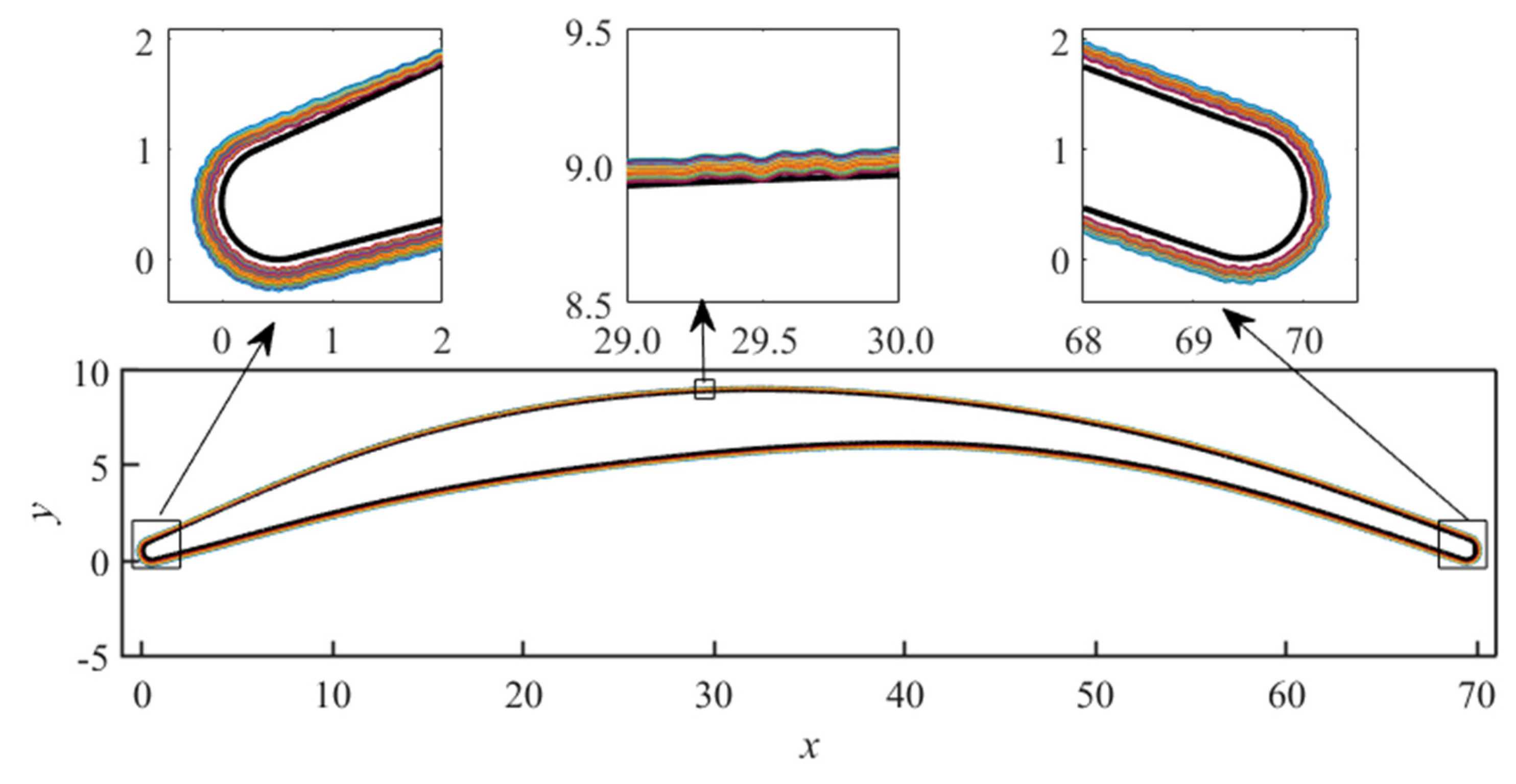
2.5. Methods for Modeling Fouling Blades

The geometric coordinates of fouling blade can be obtained by superimposing the fouling values obtained by the above modeling method in the normal direction to the coordinates of the original blade, the principle of which is shown in Figure 4. The black curve in the figure the partial outline of the blade suction surface and points A and B are two adjacent coordinate points with close distance on the blade suction surface, and the vector formed by them is $\overrightarrow{a}$. When the size l of the fouling is known, the vector $\overrightarrow{b}$ perpendicular to the vector $\overrightarrow{a}$ can be determined. The following calculation method is used to obtain the fouling blade profile coordinate point C relative to the clean blade profile coordinate point A.

Based on the coordinate points A and B, the angle θ between the vector $\overrightarrow{a}$ and the horizontal can be calculated by Equation (25). Since vector $\overrightarrow{a}$ is orthogonal to the vector $\overrightarrow{b}$, the angle between a vector $\overrightarrow{b}$ and the vertical direction is θ. In turn, based on the data of the original coordinates A, the fouling blade coordinate point C can be obtained through Equations (16) and (17). In this way, the coordinates of each point on the clean blade can be obtained after the fouling blade, and the smooth connection of the coordinate points can be used to generate the fouling blade profile.

$$\theta =\mathrm{a}\mathrm{r}\mathrm{c}\mathrm{t}\mathrm{a}\mathrm{n}{\displaystyle \frac{y_2-y_1}{z_2-z_1}}$$

(15)

$$z_0=z_1\pm \mathrm{s}\mathrm{i}\mathrm{n}(\theta ·y)$$

(16)

$$y_0=y_1\pm \mathrm{s}\mathrm{i}\mathrm{n}(\theta ·y)$$

(17)

2.6. Verification of Uncertainty Model of Fouling Rough Structures

To illustrate that the model proposed in this paper is sufficient to characterize the fouling distribution and morphology, it should be verified. As mentioned previously, the dense fouling layer is used to characterize the distribution of blade fouling, and the loose fouling layer is used to characterize the morphology of blade fouling. The dense fouling layer model is mainly determined by the mean and standard deviation of fouling distribution on the blade surface, so the most important thing is to verify whether the loose fouling layer model can represent the rough structures of fouling.

2.6.1. The Control Parameters in the FLH Model

To characterize the roughness of the uncertainty of the loose fouling layer, the FLH model (Equation (11)) in Section 2.3 is used to describe its roughness morphology. Based on the relevant literature, the roughness of the established rough structures of the loose fouling layer is determined, and the relevant control parameters in the FLH model are regulated according to the target roughness value, to establish a model for the uncertainty of the loose fouling layer morphology. Therefore, the effect of parameter settings in the FLH model on the modeling results will be further investigated while the roughness Ra = 20 µm, which means a_n is confirmed.

The parameter $N_f$ in the FLH model determines the dimensions of the variables for uncertainty modeling, which directly determines the number of uncertainty models of the loose fouling layer morphology constructed. Accordingly, the effect of the value of $N_f$ on the modeling results must be evaluated. The smaller $N_f$ is, the smaller the number of models is. Nevertheless, a smaller $N_f$ will lead to the loss of irregular features in the rough structures, and will not be able to correctly characterize the irregular roughness of the loose fouling layer. Therefore, it is crucial to determine a suitable value of $N_f$ to ensure that the modeling results can describe the irregular roughness while generating the smallest possible number of models and reducing the computational effort.

Figure 5 shows the effect of $N_f$ on the rough structures at Ra = 20 µm. It can be found that the rough structures have obvious periodic characteristics when $N_{f }$= 1 and 2, which is not consistent with the irregular rough structures that need to be established in this study, so it is not considered. The periodicity of the rough structures is weakened when $N_f$= 3, it is noted that the periodicity still exists through the local magnification. However, the roughness is no longer periodic when $N_f$= 4, and the waveforms composed of the roughness features begin to have skewed features, and as $N_f$ increases to 5, the irregular roughness features become more obvious, and the skew of the waveform further increases. However, when $N_f$ is increased to 6, although the constructed rough structures have irregular rough features, it can be found that the features of the rough structure are only different from the amplitude and phase when $N_f$= 5 by the local magnification of the figure. It indicates that increasing $N_f$ is not beneficial for obtaining more abundant waveforms, while increasing the dimension of independent variables leads to increased computing costs. Therefore, $N_f$= 5 is the minimum value to characterize the rough structures of the loose fouling layer.

The uncertainty of particle size and shape affects the uncertainty of the rough structures of the compressor blade fouling, and the effect of this uncertainty on the rough structures is mainly reflected in the size of the wave distance, so it is meaningful to explore the effect of the wave spacing control parameter ω_n on the rough structures of fouling.

To characterize the uncertainty of the rough structures, a standard normal distribution is used to randomly generate ϵ. When $N_f$ is determined, the parameter ω_n can be regulated to achieve the rough structures of the loose fouling layer with different wave distances, which will be directly influenced by the coefficient c, as shown in Equation (12). While ϵ is constant, the greater c is the rougher the calculated loose fouling layer morphology, and the higher the roughness frequency the smaller the wave distance. The selection of parameter c must take into account the size range of the particles (0–20 μm) forming the fouling [14] and the richness of the rough structures. The effect of the coefficient c on the wave distance of the rough structures is given in Figure 6 while Ra = 20 μm. What is most obvious is that the wavelength λ_rough of the rough structures decreases as c increases, and the more abundant the rough features are from Figure 6a–e.

It is worth noting that the wavelength λ_rough of the rough structures exceeds 1000 μm when c = 1 and 5, which is far from the actual fouling rough structures, as shown in Figure 6a,b. When c is increased to 15, the wavelength λ_rough decreases significantly, and by sampling the wavelength of the rough structures randomly, it is found that the wavelengths λ_rough are not completely consistent at different locations, which reflects the uncertainty characteristics of the rough structures of the loose fouling layer. As c continues to increase to 20, the wavelengths of the rough structures are almost always below 100 μm, which is more in keeping with the characteristics of the rough structures of real blade fouling. Naturally, as c increases to 30, the wavelength λ_rough of the rough structures is smaller, which means that the grid needs to be much finer when carrying out CFD calculations to be able to adequately characterize such a slight variation. Therefore, it is necessary to choose appropriate parameters c to ensure the simulation of more realistic roughness characteristics and facilitate CFD calculations when establishing the roughness model of the loose fouling layer.

Figure 7 shows the influence of the skew direction control parameter ${\vartheta }_n$ on the rough structures, and the lines with different colors represent the rough structures of the loose fouling layer established by different parameters ${\vartheta }_n$ of Gaussian distribution. It can be found that the effect of changing ${\vartheta }_n$ on the roughness and the wavelength λ_rough of the rough structures is not significant when other parameters are constant. Three gray lines perpendicular to the x-axis have been drawn at each of the three positions in Figure 7 to observe more clearly the effect of the random variation of the parameter ${\vartheta }_n$ on the skewness of the rough structures at the same position. It can be found that the skewness of the rough structures is completely different for different values of the parameter a at the same position. Therefore, it is possible to construct a model of a loose fouling layer with random morphology by modulating the skew direction control parameter ${\vartheta }_n$ when the other control parameters are consistent. In addition, the variation of ${\vartheta }_n$ affects the roughness within ±1 μm when other control parameters are conserved constants, which is within the viscous sublayer of the compressor blade flow field and has almost no effect on the flow field.

To sum up, the FLH model can be adjusted to achieve the establishment of the rough structures model of the dense fouling layer and ensure that the established model has randomness and rough structure characteristics. Most importantly, the rough surface structures established by the FLH model are discontinuous, which effectively characterizes the discontinuous rough surface morphology of fouling caused by particle accumulation.

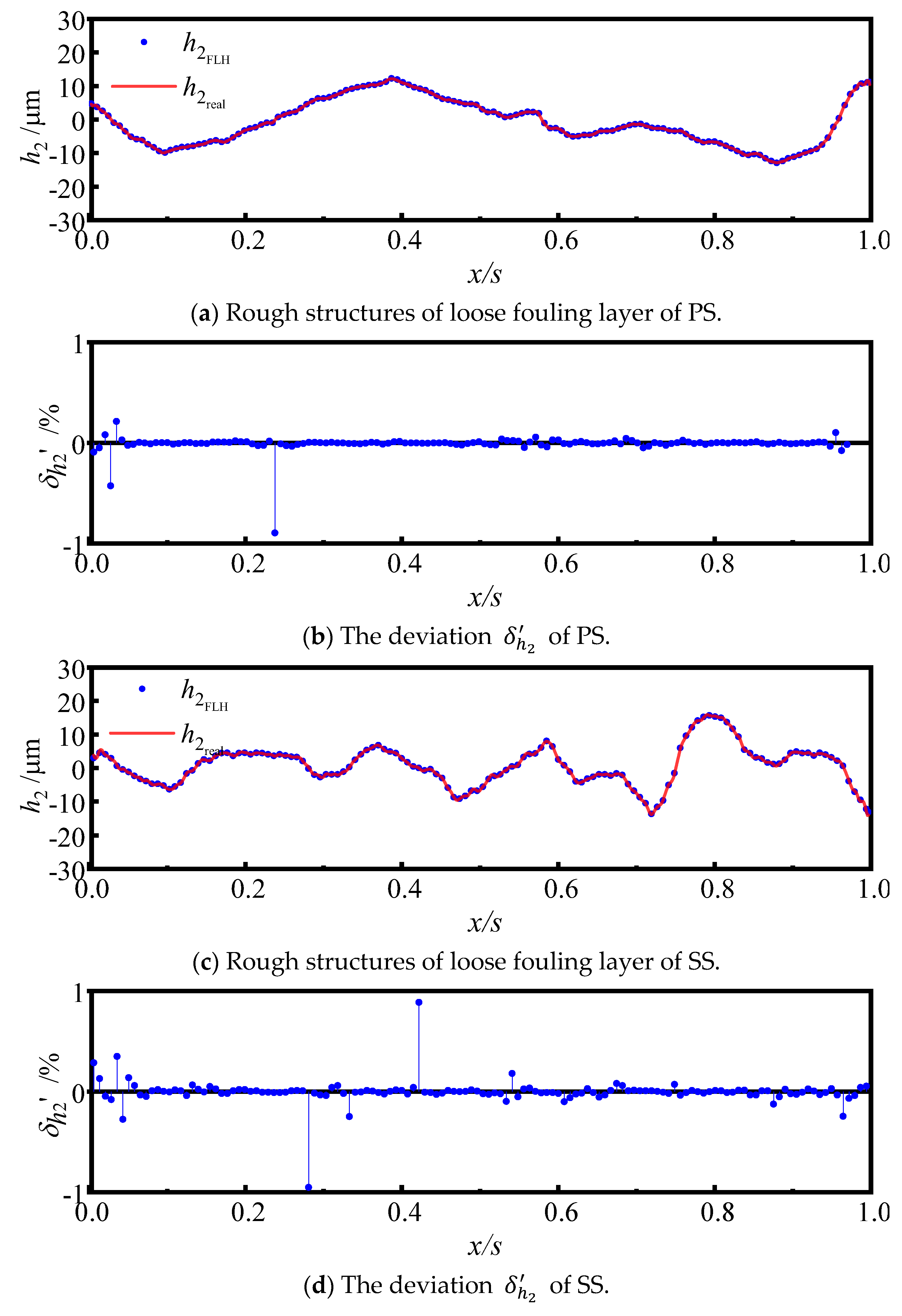
2.6.2. Validation of the FLH Model

The measurement data [13,34] of the real blade fouling after service show that the fouling morphology of the blade surface is irregular and rough, and has certain skew characteristics, and the fouling morphology is completely different in the different blade height sections of the same blade and the same cross-section of different blades. Therefore, it is important to show that the FLH model can characterize the fouling morphology of irregular rough structures and that the skewed features of the fouling morphology are reasonably well characterized.

A set of rough structures scans of real compressor blade fouling is employed as a standard for calibrating the FLH model, and the specific rough structures of fouling [13] are shown in Figure 8. The fouling rough structures at different cross-sections and locations are chosen, and Figure 8a shows the rough structures of PS at 7.5 mm from the hub section, and Figure 8b shows the rough structures of SS at 10 mm from the hub section. Then, the FLH model is employed to construct the rough structures of the loose fouling layer shown in Figure 8.

The deviation ${\displaystyle {\delta }_{h_2}^{\prime }}$ between the loose fouling layer rough structures constructed by the FLH model and the real fouling roughness morphology of Figure 8 is calculated through Equation (18), specifically,

$${\displaystyle {\delta }_{h_2}^{\prime }}(x)=({h_2}_{FLH}(x)-{h_2}_{real}(x)/{h_2}_{real}(x)$$

(18)

The iterative method is used to solve the loose layer fouling thickness $h_{2_{FLH}}$ in the FLH model until the deviations ${\displaystyle {\delta }_{h_2}^{\prime }}$ are sufficiently small and adequate to characterize the rough structures. The specific calculation results are shown in Figure 9. The blue dots are the fouling roughness data simulated by the FLH model, and the red line is the roughness of fouling on a real compressor blade as shown in Figure 9a,c. It can be found that the FLH model can better simulate the rough structure characteristics of fouling on compressor blades and different rough structures can be simulated at different locations through continuous iteration. Moreover, it can be better characterized by the roughness, skewness, and other features of the real fouling morphology. Similarly, the deviation ${\delta }_{h_2}^{\prime }$ of the fouling rough structures simulated by the FLH model is demonstrated in Figure 9b,d, with the blue dots being the percentage deviation. It can be noted that the deviation ${\delta }_{h_2}^{\prime }$ of the fouling rough profile is within ±1% for both simulated PS and SS.

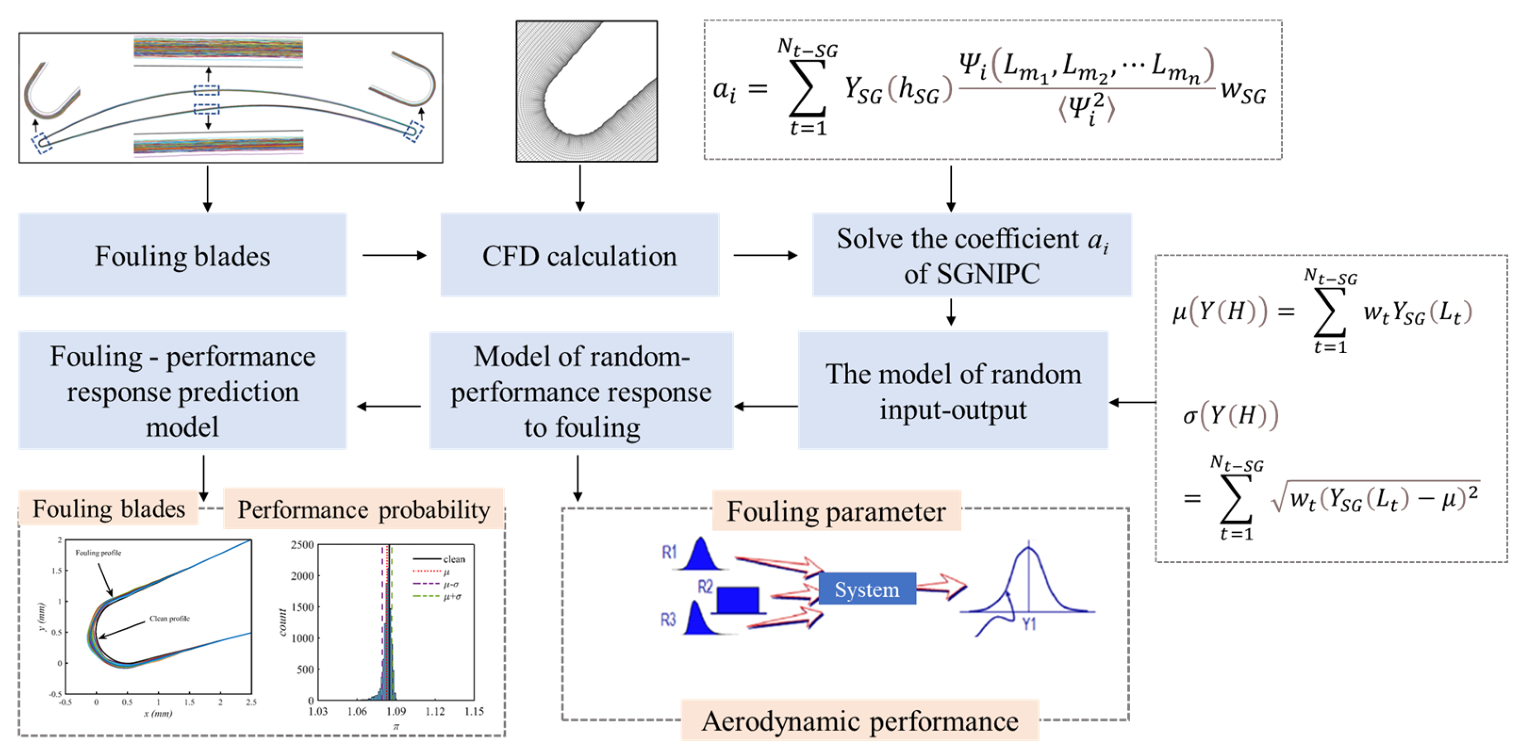
2.7. Sparse Grid Non-Intrusive Polynomial Chaos (SGNIPC)

Non-intrusive Polynomial Chaos (NIPC) is a stochastic spectral method with high prediction accuracy and uncertainty quantification (UQ) efficiency, which greatly reduces the number of simulations for predicting stochastic output moments in CFD simulations, compared to classical UQ methods. The times N_t that the CFD is invoked are determined by the number of random variable dimensions n and integration nodes m in each dimension, and increases exponentially with n as m increases. Therefore, the full factorial numerical integration (FFNI) is only applicable to problems with n < 5, and the problem of NIPC computational surge triggered by n ≥ 5 is solved by the sparse grid non-intrusive polynomial chaos (SGNIPC) method developed in previous research [46].

In this study, the SGNIPC method is employed to quantify the effect of fouling on the aerodynamic performance of compressor blades to better balance the computational efficiency and computational accuracy. The SGNIPC method utilizes a set of orthogonal polynomials and their corresponding deterministic coefficients to construct the system response Y_SG to a random variable h_SG. The transfer function is Y_SG(h_SG)

$$Y_{SG}\left(h_{SG}\right)={\displaystyle {\sum }_{i=0}^{Q-1}}{a}_i{\Psi }_i\left(h_{SG}\right)$$

(19)

$$Q={\displaystyle \frac{\left(n+p\right)!}{n!p!}}$$

(20)

where Ψ_i(h) is the product of the orthogonal basis functions of the random variables in each dimension, which is determined by the type of the probability density function of the random variables. Q represents the number of terms of the orthogonal polynomial, as determined by the number of dimensions of the random variables n and the highest order of the polynomial p.

The key to solving the uncertainty statistical characteristics of the system response Y_SG depends on solving the NIPC coefficients a_i, and the Galerkin projection method has the advantages of easy computation and high accuracy in solving the coefficients of NIPC, which is as follows:

$$a_i={\displaystyle {\sum }_{t=1}^{N_{t-SG}}}{Y}_{SG}\left(h_{SG}\right){\displaystyle \frac{{\Psi }_i\left(L_{m_1},L_{m_2},\cdots L_{m_n}\right)}{〈{\Psi }_i^2〉}}{w}_{SG}$$

(21)

where < > is for the inner product, and h_SG represents the thickness of the fouling at the integral node. L_mi is the integrating node and w_t represents the corresponding weight of the sparse grid integrating node.

The corresponding system response Y_SG is also uncertain when the input random variable h_SG to the system contains uncertainty. Therefore, the mean μ and standard deviation σ, which characterize the uncertainty statistics of the system response Y, can be calculated by the following equation:

$$\mu \left(Y\left(H\right)\right)={\displaystyle {\sum }_{t=1}^{N_{t-SG}}}{w}_t{Y}_{SG}\left(L_t\right)$$

(22)

$$\sigma \left(Y\left(H\right)\right)={\displaystyle {\sum }_{t=1}^{N_{t-SG}}}\sqrt{w_t{\left(Y_{SG}\left(L_t\right)-\mu \right)}^2}$$

(23)

Therefore, combining the calculation accuracy and efficiency, this study chooses the SGNIPC method with K = p = 3 to model the geometric uncertainty of fouling and to carry out the study of the geometric uncertainty of fouling and aerodynamic performance response.

The specific quantitative method and process of the aerodynamic performance of the fouling blade are shown in Figure 10. Firstly, the fouling model established in Section 2 is divided into grids and CFD is invoked for calculation. Based on the CFD calculation results, extract the main aerodynamic performance parameters of concern and substitute them into the formula to solve the coefficient a_i of SGNIPC. When the coefficient a_i is solved and substituted into Formula (19), the mean and standard deviation of the aerodynamic performance parameters of the fouling cascade can be obtained. Therefore, the correlation model between the random fouling parameters and the aerodynamic performance response has been established. Finally, based on the established model between random fouling and aerodynamic response, the aerodynamic performance degradation of fouling compressor blades can be predicted.

3. Research Object and Research Scheme

3.1. Research Object

The fact is that this blade was independently developed by the group and has been subject to a substantial amount of experimental and numerical studies in previous research [47,48]. Figure 11 is the two-dimensional compressor blade of NUP-A1 with a leading edge radius of 0.5205 mm and a chord length of 69.95 mm. The design stagger angle is 26.58°, the pitch is 30.4350 mm, and the maximum thickness (c_max) is 3.5127 mm.

3.2. Numerical Simulation Methods

The irregular rough structures of the fouling blade have an obvious effect on the flow pattern of the surface attached layer of the blade, especially the transition process of the laminar attached layer to the turbulent attached layer. Therefore, the numerical simulation method in this paper adopts the SST turbulence model coupled with the γ-Re_θ transition model, which has a better ability to capture the transition position and has been widely used in the study of the development of flow patterns in the attached surface layer of the diffuser cascade [49,50]. In addition, the accuracy of the NPU-A1 blade calculated using this turbulence model has been verified in previous studies [51], as shown in Figure 12.

In the previous verification study, it was found that the accuracy of the SST + γ -Re_θ turbulence model in calculating the total parameters of aerodynamic performance is in good agreement with the experiment, so the SST + γ -Re_θ turbulence model can be used to study the total performance degradation and transition of fouling cascade.

3.3. The Scheme of Fouling Modeling

The operating conditions and blade shape mainly change the aerodynamic loading of the blades, which further affects the distribution of blade fouling. It has been indicated that particles are more likely to be deposited in the low-speed region [52]. Based on the measurement results of an aero engine compressor blade fouling after a test flight and the trend of fouling distribution obtained in previous studies [5,12,13,14,15,16,17], it can be found that the fouling is thicker at the leading edge, the amount of fouling from the leading edge to the trailing edge in the suction surface is decreasing and then increasing, and there is always a thicker fouling in the pressure surface and the trailing edge. Therefore, the current study referred to the existing literature for the measurement of the real fouling distribution and the theory of particle deposition [53,54] combined with the location of the control points.

In the existing studies for CFD calculations on rough surfaces, it was found that when the height of the rough element is smaller than the thickness of the viscous sublayer, its effect on aerodynamic performance is indistinguishable from CFD calculations [37]. This means that the effect of rough structures on the flow field cannot be obtained from CFD calculations when the modeling scale of the loose fouling layer is smaller than the thickness of the viscous sublayer. Therefore, in this study, the thickness of the viscous sublayer and the particle size in existing studies are considered to construct the rough structures of the loose fouling layer.

The cases of all the incidences are calculated for the NPU-A1 blade at Ma = 0.5, and the mean viscous sublayer thickness δ′ is shown in Figure 13. It can be found that the minimum thickness of the leading edge viscous sublayer is only 3 µm, which means that the effect on the flow field of the leading edge loose fouling layer cannot be obtained by CFD calculations when the modeling scale of the fouling is less than 3 µm. Meanwhile, to study the effect of the fouling roughness on the perturbation of the flow field, it should be ensured that the loose fouling layer modeling crosses the viscous sublayer. In addition, particle size [14] has a major impact on the morphology of the loose fouling layer, and the particle size of the fouling-forming particles must be taken into account while modeling the loose fouling layer.

To validate the developed modeling approach and aerodynamic performance uncertainty quantification method, verification was conducted for both fouling thickness uncertainty and roughness structure randomness. The modeling dimensions and scales were determined based on fouling measurement data obtained from endurance testing of a specific engine compressor in previous research by the group. The measurements revealed that fouling thickness on blade surfaces primarily ranged from 10 µm~160 µm. Since the primary focus of this study lies in the modeling methodology and uncertainty quantification framework, a representative thickness of 50 µm within this measurement range was selected for investigation. Detailed analyses of uncertainty in fouling distribution patterns and roughness structure scales will be addressed in subsequent studies.

4. Case Validation and Analysis

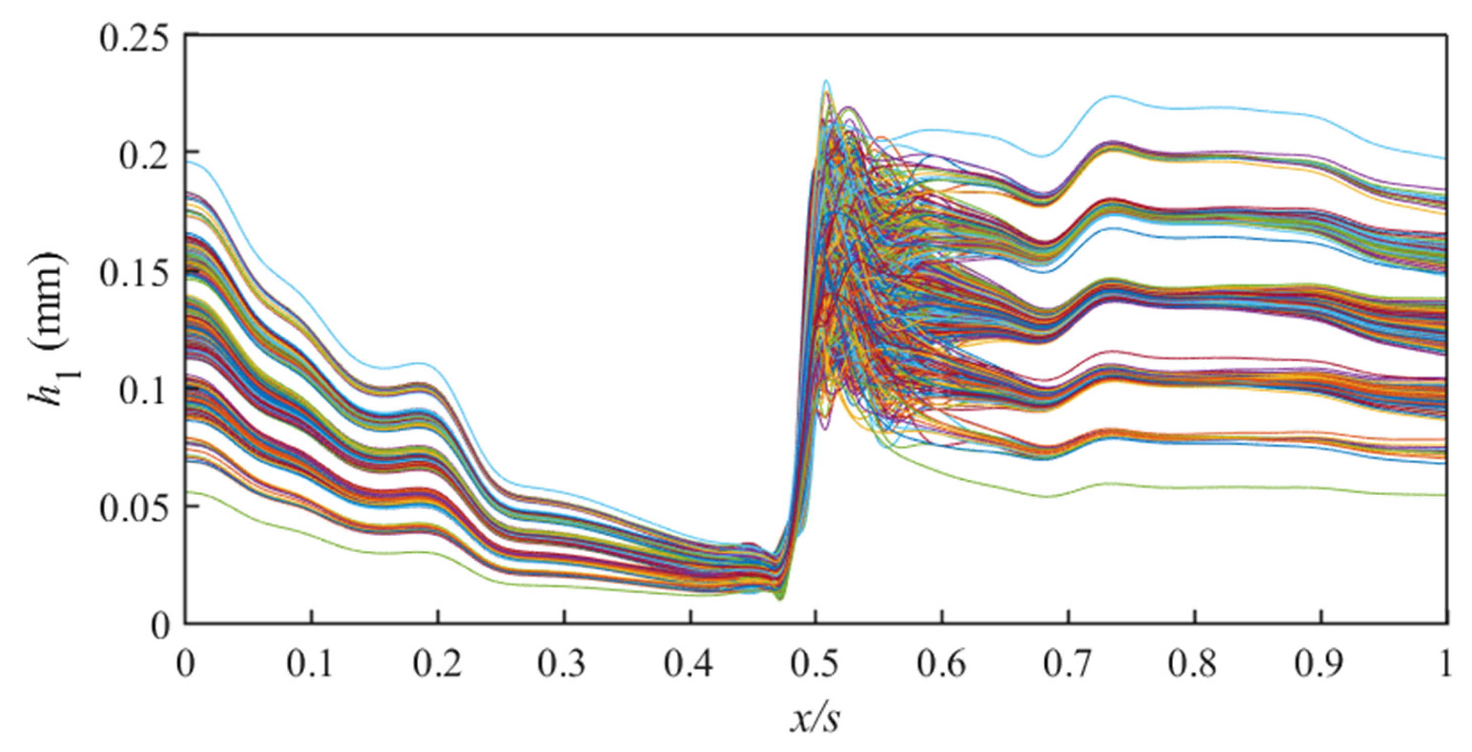
4.1. Thickness Uncertainty Modeling of Blade Fouling

The number of control points on the blade profile directly affects the modeling quantity of the dense fouling layer and computational efficiency, so it is very important to select a suitable number of control points.

It is essential to determine the number of control points at the leading edge. Due to the high aerodynamic sensitivity of the leading edge and its susceptibility to fouling, it is necessary to arrange reasonable control points to describe the variation in the dense fouling layer at the leading edge to ensure modeling accuracy while reducing the number of models. It has been shown that the location of the maximum thickness of fouling at the leading edge mainly shows two distribution trends of biased suction and pressure surface [13], and this paper is a circular leading edge, so five control points are selected at the leading edge for describing the variation in the dense fouling layer. Similarly, five control points are used for the trailing edge. The number of control points on the suction and pressure surfaces should not only fit the design blade profile but also describe the trend of fouling along the blade profile. Therefore, 15 control points are used to fit the suction and pressure surface blade profile lines, which are found to fit the design blade profile better.

The design blade profile and the fitted blade profile using the above control points are given in Figure 14. It can be found that the blade profile is well fitted while the number of control points in both suction and pressure surfaces is 15, as shown in Figure 14a. However, the fitted profile deviates from the design blade profile when the number of control points is reduced to 14, especially at the suction surface position, as shown in Figure 14b. Therefore, 15 control points are selected for each of the suction and pressure surfaces for modeling the dense fouling layer. With this, a total of 40 control points have been selected to model the dense fouling layer for the entire blade profile.

It is possible to obtain the mean and standard deviation of the fouling at the control point locations according to the distribution of fouling on the blade surface once the number of control points and the locations of the control points have been determined, which can be used to construct the covariance matrix C_cov in Equation (6), and then to establish the dense fouling layer model.

As mentioned above, the mean ($\overline{h_1}$) and standard deviation (${\sigma }_{h_1}$) of fouling accumulation at each control point location are constructed based on the existing distribution trends of fouling, the distribution of the dense fouling layer along the blade arc is obtained, as shown in Figure 15. For clarity, h_1c is introduced to denote the relative magnitude of the dense fouling layer thickness, defined as the ratio of fouling thickness to the maximum cascade thickness (c_max), with the specific formula given by

$$h_{1c}=h_1/c_{\max }$$

(24)

The black line in Figure 15 represents the mean value $\overline{h_1}$ of the dense fouling layer and the gray shading represents the standard deviation ${\sigma }_{h_1}$. It can be found that $\overline{h_1}$ of the thickness of the fouling in the dense layer decreases and then increases from the leading edge (LE) to the trailing edge (TE) in the suction surface (SS), and is larger in the pressure surface (PS). Similarly, the standard deviation ${\sigma }_{h_1}$ follows the same trend as the mean along the arc of the blade. It should be noted that for this study, the blade arc coordinates are separated along the trailing edge points and normalized along the trailing edge, suction surface, leading edge, and pressure surface directions. It should be noted that the mean relative thickness of the dense fouling layer h_1c ranges from 0.0066 to 0.0448.

It is then a matter of choosing the appropriate truncation percentage based on the constructed covariance matrix to reduce the modeling dimension of the dense fouling layer from 40 to M based on Equation (3). Figure 16 presents the cumulative sum of the eigenvalues of the covariance matrix of the control points of the dense fouling layer. Among them, the grey bar chart represents the cumulative sum, and the black dot chart represents the percentage of each eigenvalue. It can be found that the first 3 eigenvalues have occupied 90% of all the eigenvalues, and when the number of eigenvalues is 7 it has reached 97.5% of the sum of eigenvalues and gradually converges. Therefore, this paper chooses 97.5% as the truncation percentage, where M = 7.

Based on the dimensionality reduction result M = 6 and sparse level K = 3, the NIPC integral nodes arranged according to the full tensor are sparse (Equation (8)), and the final solution is N_t−SG = 680. The integral nodes obtained by the solution are substituted into Equation (2) to calculate the distribution of 680 dense layers of fouling thickness along the blade profile, as shown in Figure 17. Different colors represent the calculated different thicknesses of scale deposits distributed along the chord length.

To investigate the effect of uncertainty in the thickness of the dense fouling layer on the degradation of aerodynamic performance, it is necessary to ensure that the morphology of the loose layer scale is consistent. The specific modeling methods and parameters of the dense layer fouling and loose layer scale are described in Section 2.3. Figure 18 shows the uncertainty model of the thickness of the 680 compressor blades’ dense layer, and different colors represent the blades under different fouling distributions and morphologies.

4.2. Rough Structure Uncertainty Modeling of Blade Fouling

Therefore, in this study, the selection of $N_f$= 5 can satisfy the regulation requirements of each control parameter, which can completely realize the construction of irregular roughness while ensuring a low variable dimension. The parameter c = 15 was chosen so that the wavelength of the rough structures of the loose fouling layer could both characterize the rough structures and facilitate CFD calculations. Parameters $ϵ$ and ${\vartheta }_n$ obey a standard Gaussian distribution and their nodes in the Gaussian distribution are calculated by Equation (10), and the parameter ${\epsilon }_n$ is a set of random numbers obeying a uniform distribution. Similarly, h_2c represents the relative roughness of the loose fouling layer, defined as the ratio of fouling roughness Ra to the maximum cascade thickness (c_max). The calculation formula is

$$h_{2c}=h_2/c_{\max }$$

(25)

From the above, the uncertainty model of the loose fouling layer with Ra = 50 μm is constructed in this paper, as shown in Figure 19. The relative value h_2c range of the roughness of the loose layer fouling is 0 to 0.01424. To characterize the rough morphology of the fouling, a total of 7375 points were selected on the arc length of the blade as modeling variables. Among them, the maximum distance between two points on the arc length was 19 μm, which was sufficient to characterize the rough morphology of the peaks and troughs on the surface of the fouling blade, and different colors represent the different fouling morphologies.

It can be found that the uncertainty of the rough structures of the loose fouling layer is mainly reflected in the randomness of the wavelength, the randomness of the peaks and valleys, and the inconsistency of the skew direction, which are similar to the rough characteristics of the compressor blade fouling, and which are sufficient to characterize the uncertainty features of the roughness of the loose fouling layer for the compressor blades.

Similarly, even if the roughness is constant, the rough structures will not be completely consistent due to the influence of particles and incoming flow conditions. It is worth studying how much the uncertainty of rough structures affects aerodynamic performance. Therefore, it is ensured that the trend of the thickness distribution of the dense fouling layer is consistent, and the uncertainty of the loose layer roughness and morphology is modeled. The uncertainty model for the blade with consistent roughness and inconsistent morphology is given in Figure 20, and different colors represent the blades under different fouling distributions and morphologies. The thickness distribution of the dense fouling layer is the mean value at each control point, and the modeling parameters for the loose fouling layer are given in Section 4.1.

As mentioned above, the uncertainty of the blade surface fouling mainly consists of the uncertainty of the thickness of the dense fouling layer and the uncertainty of the rough structures of the loose fouling layer. To investigate the effect of these two types of fouling uncertainties on the degradation of aerodynamic performance, these two types of fouling uncertainties need to be investigated separately. Therefore, the aerodynamic performance is quantified for the thickness uncertainty model of the dense fouling layer and the rough structures uncertainty model of the loose fouling layer, respectively.

4.3. Numerical Method of Fouling Cascade

The SST turbulence model coupled with the γ-Re_θ transition model has to ensure the y + <1. Based on the above turbulence model, the extension distance of upstream and downstream is 1.0 axial chord length and 2.5 axial chord length, respectively, as shown in Figure 21. The inlet boundary condition is given by the inlet total temperature and pressure, the outlet boundary condition is given by the mean static pressure, and the corresponding Mach number is achieved by adjusting the outlet static pressure. The inlet turbulence intensity is specified at 5%, the walls are treated as adiabatic no-slip walls, the working fluid is an ideal gas, and its compressibility is accounted for.

The specific fouling cascade grid is shown in Figure 21, with locally enlarged views of the grid at the leading edge, mid-span, and trailing edge regions. It can be observed that the grid resolution is sufficient to characterize the microscopic structures on the blade surface. A grid independence verification was performed, demonstrating that a grid containing 3.2 × 10⁵ nodes achieved grid-independent results.

4.4. Aerodynamic Uncertainty Response of Blade Fouling

Numerical simulations are carried out based on the uncertainty model of the dense fouling layer thickness established in Section 4 for the case of Ma = 0.5, i = 0°, and the coefficients of NIPC are calculated based on Equation (19). The probability density distribution of aerodynamic performance under the influence of the uncertainty of the thickness of the dense fouling layer is also calculated using 10⁴ Monte Carlo results, as shown in Figure 22. It should be noted that the histograms of the frequency distributions of the static pressure ratio and total pressure loss coefficients show peaked or skewed characteristics, which are quite different from the Gaussian distribution of the input variables. Compared to the clean blade, the mean value of static pressure ratio is reduced by 0.65% and losses are increased by 39.81% due to the dense fouling layer at Ma = 0.5, i = 0°. In addition, it can be found that the uncertainty of dense fouling layer thickness makes the probability of aerodynamic performance 75.8% lower than that of a clean blade.

As mentioned above, the effect of morphology uncertainty of loose fouling layer with roughness of 50 μm on aerodynamic performance was studied for Ma = 0.5 and i = 0°. The probability density distribution of aerodynamic performance under the influence of the loose fouling layer is calculated using 10⁴ Monte Carlo results, as shown in Figure 23. Similarly to the aerodynamic performance degradation caused by dense fouling layer, the histograms of the frequency distributions of pressure ratios and losses show peaked or skewed characteristics. Compared with clean leaves, the static pressure decreases by 0.92% and the loss increases by 54.96% for the case of Ma = 0.5, i = 0°. In addition, it can be found that the probability of aerodynamic performance degradation caused by the morphology uncertainty of the loose fouling layer is 97.2% when the roughness is 50 μm. However, it is worth noting that compared with a dense fouling layer, the degradation degree of aerodynamic performance caused by a loose fouling layer is intensified, but the performance is more concentrated.

5. Conclusions

To simulate the uncertainty of the distribution and morphology of fouling on compressor blades, this paper develops an uncertainty modeling method for the compressor blades fouling by combining the sparse grid chaotic polynomial expansion method, establishes the uncertainty model for compressor blade fouling, and investigates the uncertainty effect on the aerodynamic performance, with the specific conclusions as follows:

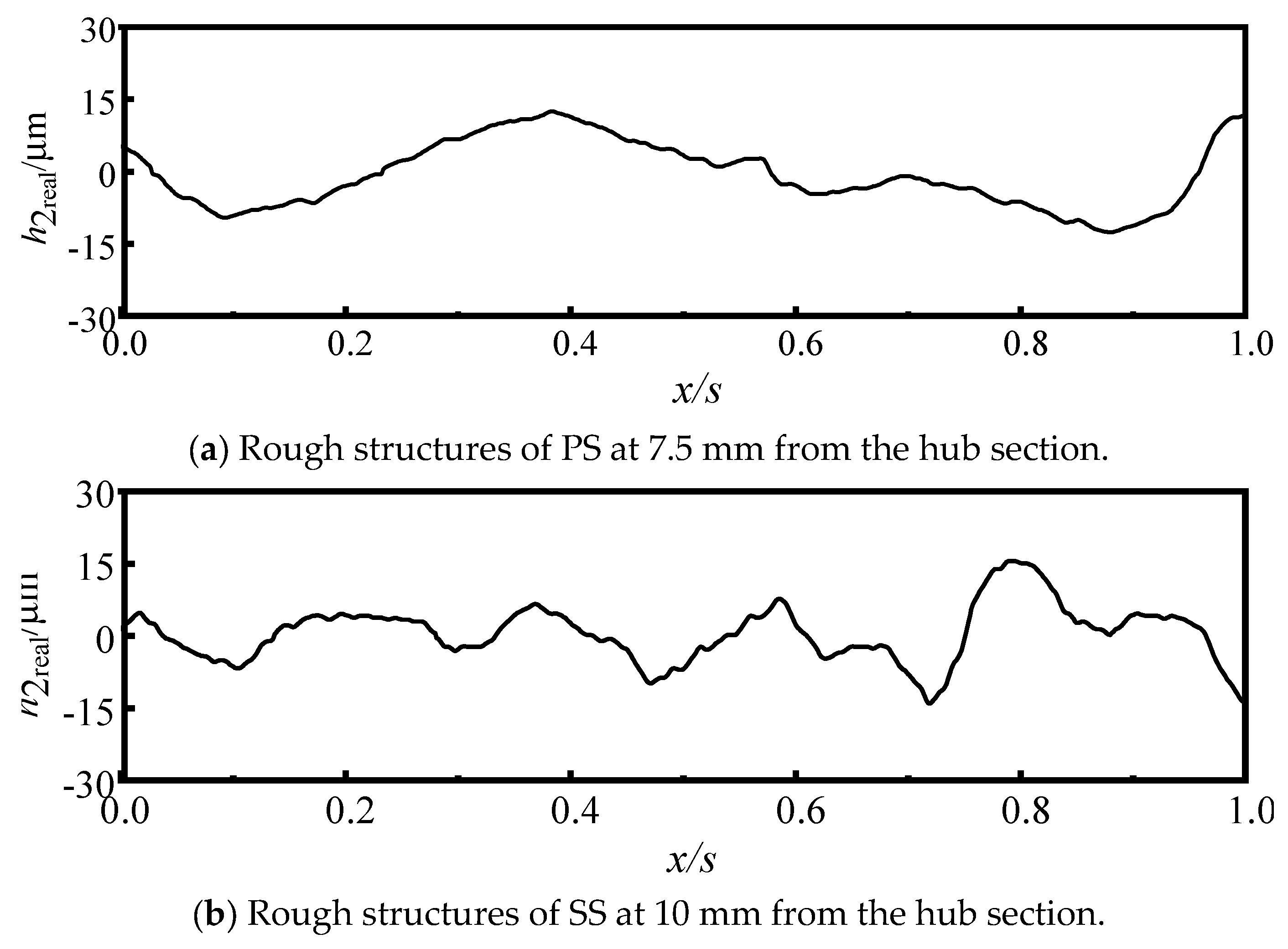
• Considering the uncertainty of operating conditions and particle size distribution, the mathematical description method of compressor blade fouling is proposed, which is divided into the thickness of the dense layer and the rough structures of the loose layer. Based on the sparse grid numerical integration and KL expansion method to construct the uncertainty model of the thickness of the dense fouling layer for the compressor blade, and the FLH model is proposed to describe the size of the loose fouling layer roughness and the uncertainty of the rough structures. Using a two-dimensional cascade as the test case, a geometric uncertainty model for a fouling compressor cascade was developed based on the aforementioned modeling approach, demonstrating the feasibility of the methodology. The FLH model has been validated using actual fouling morphology and found to describe fouling with different rough characteristics. Due to the exponential growth in the number of geometric uncertainty models for fouling blades with increasing dimensionality, a 3D compressor blade fouling geometric uncertainty model has not yet been established. Future work will extend this methodology to three-dimensional fouled blades.
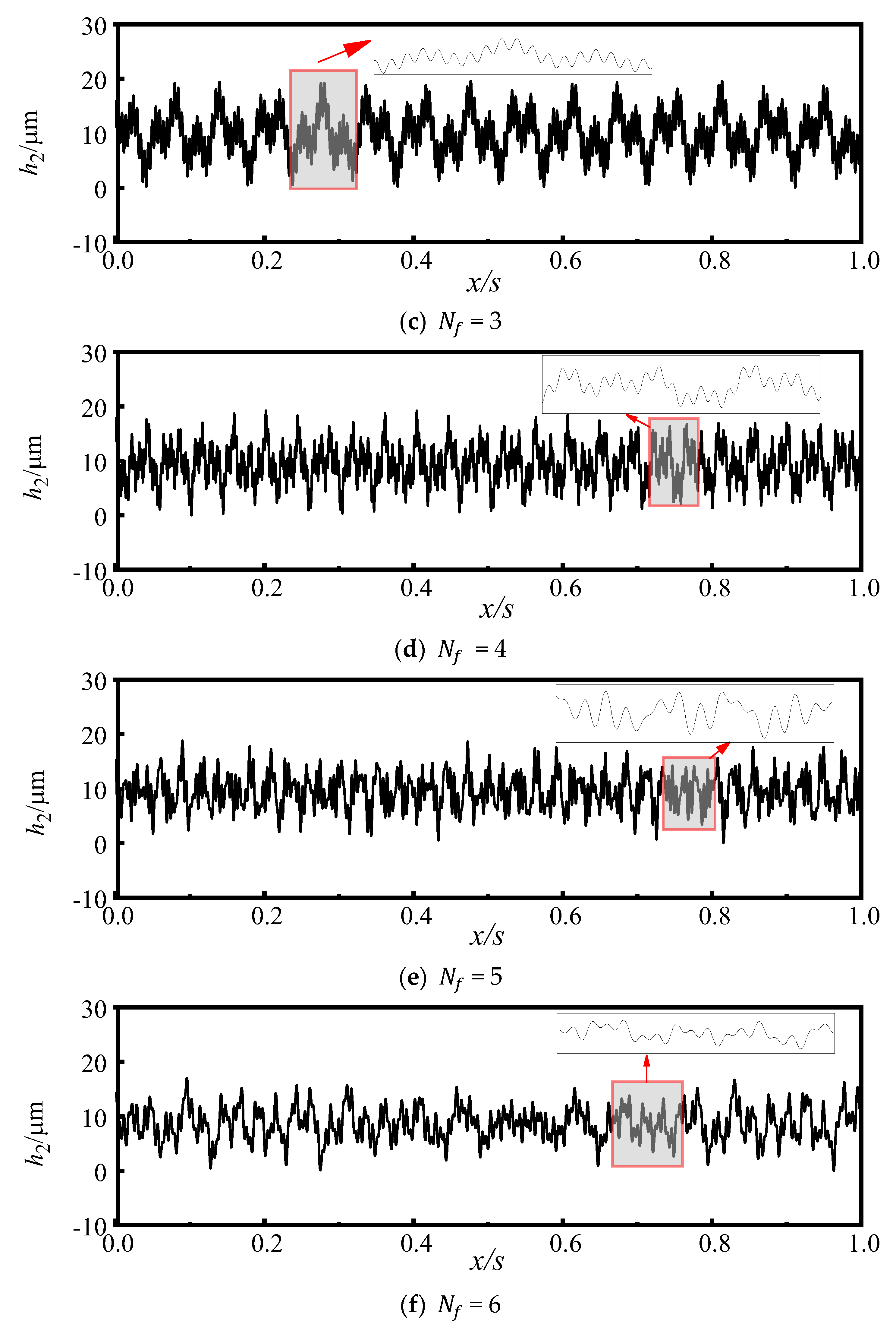
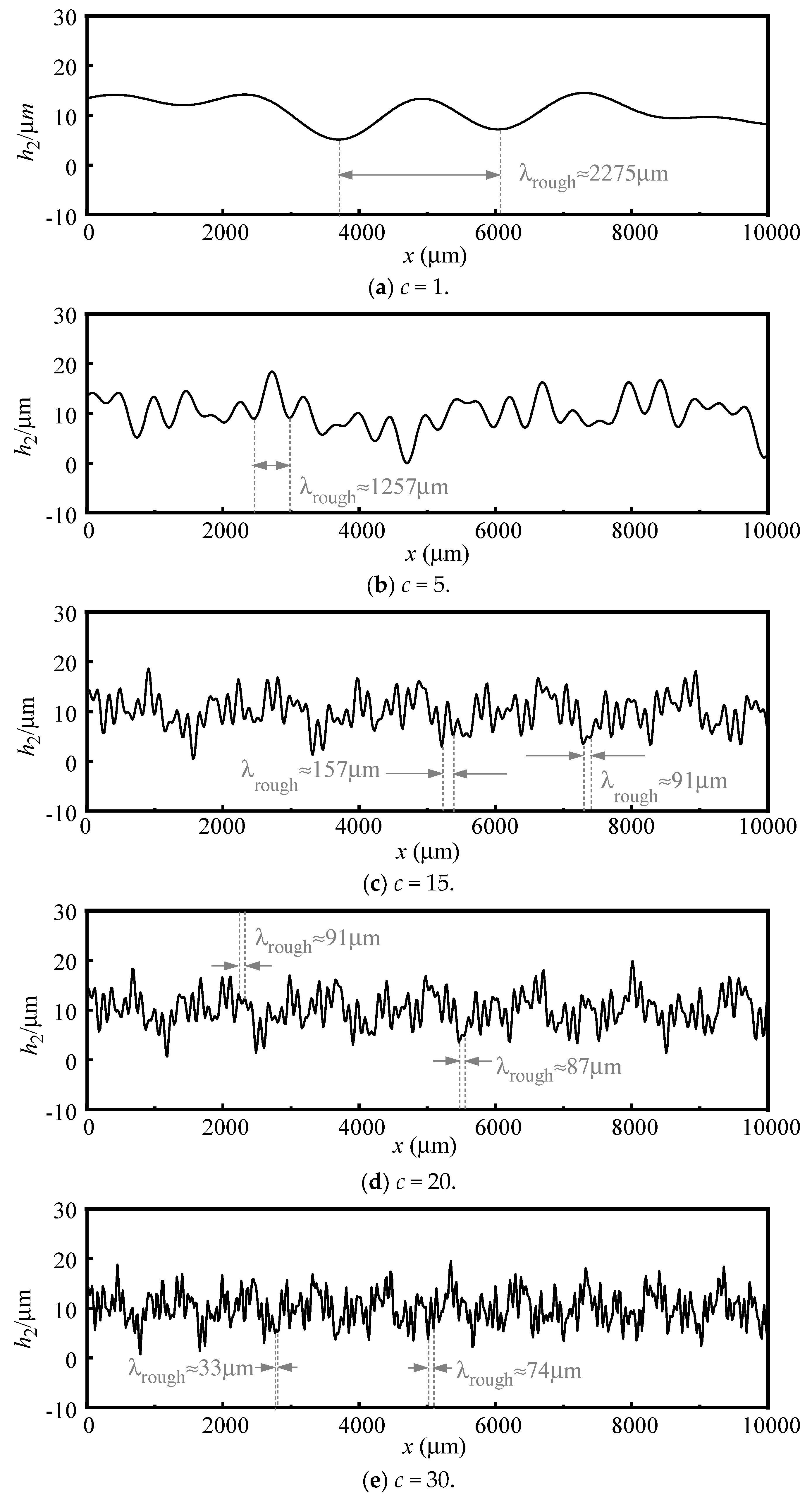
• Considering the uncertainty characteristics of the fouling rough structures, the influence law of the control parameters of the FLH model on the roughness of the loose fouling layer is given. When the wavelength control parameters of the rough structure follow a Gaussian distribution, it is guaranteed that the larger a_n is, the greater the roughness is, and the larger c is, the rougher the model is and the smaller the wavelength between the two wave peaks is when other parameters are kept constant. In addition, the parameter ${\vartheta }_n$ is adjusted to achieve the skew feature and randomness with the same roughness of the rough structures for the loose fouling layer. In addition, the variation of ${\vartheta }_n$ affects the roughness within ±1 μm when other control parameters are conserved constants.
• A method based on the sparse grid chaotic polynomial expansion of the uncertainty fouling model and aerodynamic performance uncertainty response of compressor blade fouling was developed. Assuming both fouling thickness and the wavelength control parameters of fouling roughness structures follow Gaussian distributions, the quantification of the aerodynamic performance uncertainty of compressor blade fouling in dense fouling layer and loose fouling layer was carried out. The results showed that there is a 75.8% probability of aerodynamic performance degradation due to the dense fouling layer, and the probability of aerodynamic performance degradation caused by the morphology uncertainty of the loose fouling layer is 97.2% when the roughness is 50 μm. It is further illustrated that rough structures have a large impact on aerodynamic performance degradation, and therefore it is not sufficient to describe blade fouling in terms of roughness alone; the effect of rough structures on aerodynamic performance must also be considered. With advancements in measurement technology, future research will yield more fouling morphology data from service-exposed blades. The statistical distribution characteristics of this data and its impact on aerodynamic performance degradation can be effectively analyzed using the methodology developed in this study.

References

1. Doring, F.; Staudacher, S.; Koch, C.; Weißschuh, M. Modeling particle deposition effects in aircraft engine compressors. J. Turbomach. 2017, 139, 051003. [Google Scholar] [CrossRef]
2. Igie, U. Gas Turbine Compressor Fouling and Washing in Power and Aerospace Propulsion. J. Eng. Gas Turbines Power 2017, 139, 122602. [Google Scholar] [CrossRef]
3. Giesecke, D.; Igie, U.; Pilidis, P.; Ramsden, K.; Lambart, P. Performance and Techno-Economic Investigation of On-Wing Compressor Wash for a Short-Range Aero Engine. In Proceedings of the ASME Turbo Expo 2012: Turbine Technical Conference and Exposition, Copenhagen, Denmark, 11–15 June 2012. [Google Scholar]
4. Alqallaf, J.; Teixeira, J.A. Blade roughness effects on compressor and engine performance—A cfd and thermodynamic study. Aerospace 2021, 8, 330. [Google Scholar] [CrossRef]
5. Vulpio, A.; Suman, A.; Casari, N.; Pinelli, M. Dust ingestion in a rotorcraft engine compressor: Experimental and numerical study of the fouling rate. Aerospace 2021, 8, 81. [Google Scholar] [CrossRef]
6. Bojdo, N.; Filippone, A. A simple model to assess the role of dust composition and size on deposition in rotorcraft engines. Aerospace 2019, 6, 44. [Google Scholar] [CrossRef]
7. Meher-Homji, C.B.; Focke, A.B.; Wooldridge, M.B. Fouling of Axial Flow Compressors-Causes, Effects, Detection, and Control. In Proceedings of the 18th Turbomachinery Symposium; Texas A&M University, Turbomachinery Laboratories: College Station, TX, USA, 1989. [Google Scholar]
8. Kolkman, H.J. Performance of Gas Turbine Compressor Cleaners. J. Eng. Gas Turbines Power 1993, 115, 674–677. [Google Scholar] [CrossRef]
9. Ju, Y.; Zhang, C. Robust design optimization method for centrifugal impellers under surface roughness uncertainties due to blade fouling. Chin. J. Mech. Eng. (Engl. Ed.) 2016, 29, 301–314. [Google Scholar] [CrossRef]
10. Shi, X.; Long, F.; Yan, Z.; Tang, J. A review of aero-engine blade fouling mechanism. In Proceedings of the AUS 2016-2016 IEEE/CSAA International Conference on Aircraft Utility Systems, Beijing, China, 8–14 October 2016; pp. 278–283. [Google Scholar]
11. Templalexis, I.; Pachidis, V. Simulation of Fouling in Axial Flow Compressor Using a Throughflow Method. J. Energy Eng. 2017, 143, 04016028. [Google Scholar] [CrossRef]
12. Taylor, R.P. Surface Roughness Measurements on Gas Turbine Blades. J. Turbomach. 1990, 112, 175–180. [Google Scholar] [CrossRef]
13. Mullaney, D.; Jones, M.; Bojdo, N.; Covey-Crump, S.; Pawley, A. the Effect of Additive ‘Depositional’ Reprofiling of Compressor Blade Leading Edges on Engine Performance. Proc. ASME Turbo Expo 2024, 12B, 1–12. [Google Scholar]
14. Vigueras Zuñiga M, O. Analysis of Gas Turbine Compressor Fouling and Washing on Line; Cranfield University: Cranfield, UK, 2007. [Google Scholar]
15. Syverud, E.; Brekke, O.; Bakken, L.E. Axial compressor deterioration caused by saltwater ingestion. J. Turbomach.-Trans. ASME 2007, 129, 119–126. [Google Scholar] [CrossRef]
16. Casari, N.; Pinelli, M.; Spina, P.R.; Suman, A.; Vulpio, A. Experimental Assessment of Fouling Effects in a Multistage Axial Compressor. In Proceedings of the E3S Web of Conferences; EDP Sciences, Online, 22 October 2020; Volume 197. Available online: https://www.e3s-conferences.org/articles/e3sconf/abs/2020/57/e3sconf_ati2020_11007/e3sconf_ati2020_11007.html (accessed on 26 July 2024).
17. Casari, N.; Pinelli, M.; Suman, A.; Vulpio, A. Performance losses and washing recovery of a helicopter engine compressor operating in ground-idle conditions. CEAS Aeronaut. J. 2022, 13, 113–125. [Google Scholar] [CrossRef]
18. Suman, A.; Casari, N.; Fabbri, E.; di Mare, L.; Montomoli, F.; Pinelli, M. Generalization of particle impact behavior in gas turbine via non-dimensional grouping. Prog. Energy Combust. Sci. 2019, 74, 103–151. [Google Scholar] [CrossRef]
19. Whitaker, S.M.; Peterson, B.; Miller, A.F.; Bons, J.P. The effect of particle loading, size, and temperature on deposition in a vane leading edge impingement cooling geometry. In Proceedings of the Turbo Expo: Power for Land, Sea, and Air, Seoul, South Korea, 13–17 June 2016; American Society of Mechanical Engineers: Houston, TX, USA, 2016; Volume 49798. [Google Scholar]
20. Wang, Q.; Lin, X.; Chen, D.-R. Effect of dust loading rate on the loading characteristics of high efficiency filter media. Powder Technol. 2016, 287, 20–28. [Google Scholar] [CrossRef]
21. Suder, K.L.; Chime, R.V.; Strazisar, A.J.; Roberts, W.B. The effect of adding roughness and thickness to a transonic axial compressor rotor. In Proceedings of the American Society of Mechanical Engineers, Den Haag, The Netherlands, 13–16 June 1994. [Google Scholar]
22. Suman, A.; Zanini, N.; Pinelli, M. Experimental Analysis of the Time-Wise Compressor Fouling Phenomenon. J. Turbomach. 2024, 146, 101004. [Google Scholar] [CrossRef]
23. Lei, G.; Zi-Nan, W.; Shao-Juan, G.; Hong-Wu, Z.; Chao-Qun, N. Experimental Study for Effects of Surface Roughness on Compressor Cascade Loss Characteristics. J. Propuls. Technol. 2016, 37, 1263–1270. [Google Scholar]
24. Chul Back, S.; Hobson, G.V.; Jin Song, S.; Millsaps, K.T. GT2010-22208 Effect of Surface Roughness Location and Reynolds Number on Compressor Cascade Performance; Power for Land: 2010. Available online: https://asmedigitalcollection.asme.org/GT/proceedings-abstract/GT2010/44021/121/347100 (accessed on 26 July 2024).
25. Morini, M.; Pinelli, M.; Spina, P.R.; Venturini, M. Computational Fluid Dynamics Simulation of Fouling on Axial Compressor Stages. J. Eng. Gas Turbines Power 2010, 132, 331–342. [Google Scholar] [CrossRef]
26. Laycock, R.G.; Fletcher, T.H. Time-Dependent Deposition Characteristics of Fine Coal Fly Ash in a Laboratory Gas Turbine Environment. J. Turbomach. 2012, 135, 021003. [Google Scholar] [CrossRef]
27. Wang, L.S.; Wang, Z.Y.; Wang, Y.H.; Wang, M.; Sun, H.O. Numerical simulation of low reynolds number 2-d rough blade compressor cascade. Front. Energy Res. 2022, 10, 950559. [Google Scholar] [CrossRef]
28. Sun, H.O.; Wang, L.S.; Wang, Z.Y.; Wang, M.; Wang, Y.H.; Wan, L. Simulation of the effect of nonuniform fouling thickness on an axial compressor stage performance. Adv. Mech. Eng. 2021, 13, 1–11. [Google Scholar] [CrossRef]
29. Aldi, N.; Morini, M.; Pinelli, M.; Spina, P.R.; Suman, A.; Venturini, M. Performance Evaluation of Nonuniformly Fouled Axial Compressor Stages by Means of Computational Fluid Dynamics Analyses. J. Turbomach. 2013, 136, 021016. [Google Scholar] [CrossRef]
30. Ling, W.; Gao, S.; Wang, Z.; Zeng, M.; Huang, W.; Xi, G. Direct numerical simulation of boundary layer transition induced by roughness element in a low Reynolds number compressor blade. Phys. Fluids 2024, 36, 124109. [Google Scholar] [CrossRef]
31. Clausert, F.H. Turbulent Boundary Layers in Adverse Pressure Gradients. J. Aeronaut. Sci. 1954, 21, 91–108. [Google Scholar] [CrossRef]
32. Rath, N.; Mishra, R.K.; Kushari, A. Investigation of Performance Degradation in a Mixed Flow Low Bypass Turbofan Engine. J. Fail. Anal. Prev. 2023, 23, 378–388. [Google Scholar] [CrossRef]
33. Gbadebo, S.A.; Hynes, T.P.; Cumpsty, N.A. Influence of surface roughness on three-dimensional separation in axial compressors. In Proceedings of the ASME Turbo Expo 2004: Power for Land, Sea, and Air, Vienna, Austria, 14–17 June 2004. [Google Scholar]
34. Bons, J.P.; Taylor, R.P.; McClain, S.T.; Rivir, R.B. The many faces of turbine surface roughness. J. Turbomach. 2001, 123, 739–748. [Google Scholar] [CrossRef]
35. Suman, A.; Vulpio, A.; Pinelli, M.; D’Amico, L. Microtomography of Soil and Soot Deposits: Analysis of Three-Dimensional Structures and Surface Morphology. J. Eng. Gas Turbines Power 2022, 144, 101010. [Google Scholar] [CrossRef]
36. TurnerFathi, A.B.; Tarada Fathi, F.J.B. Effects of surface roughness on heat transfer to gas turbine blades. In Proceedings of the Heat Transfer and Cooling in Gas Turbines, Bergen, Norway, 6–10 May 1993. [Google Scholar]
37. Kadivar, M.; Tormey, D.; McGranaghan, G. A review on turbulent flow over rough surfaces: Fundamentals and theories. Int. J. Thermofluids 2021, 10, 100077. [Google Scholar] [CrossRef]
38. Deng, B.; Deng, Y.; Liu, M.; Chen, Y.; Wu, Q.; Guo, H. Integrated models for prediction and global factors sensitivity analysis of ultrafiltration (UF) membrane fouling: Statistics and machine learning approach. Sep. Purif. Technol. 2023, 313, 123326. [Google Scholar] [CrossRef]
39. Azuri, I.; Rosenhek-Goldian, I.; Regev-Rudzki, N.; Fantner, G.; Cohen, S.R. The role of convolutionsl neural networks in scanning probe microscopy: A review. Beilstein J. Nanotechnol. 2021, 12, 878–901. [Google Scholar] [CrossRef]
40. Manami, M.; Seddighi, S.; Örlü, R. Deep learning models for improved accuracy of a multiphase flowmeter. Meas. J. Int. Meas. Confed. 2023, 206, 112254. [Google Scholar] [CrossRef]
41. Chen, J.; Tang, X.; Lu, J.; Zhang, H. A Compressor Off-Line Washing Schedule Optimization Method With a LSTM Deep Learning Model Predicting the Fouling Trend. J. Eng. Gas Turbines Power 2022, 144, 081005. [Google Scholar] [CrossRef]
42. Jin, Y.; Liu, C.; Tian, X.; Huang, H.; Deng, G.; Guan, Y.; Jiang, D. A hybrid model of LSTM neural networks with a thermodynamic model for condition-based maintenance of compressor fouling. Meas. Sci. Technol. 2021, 32, 124007. [Google Scholar] [CrossRef]
43. Longuet-Higgins, M.S. On the statistical distribution of the height of sea waves. J. Mar. Res. 1952, 11. [Google Scholar]
44. Grimmett, D.; Wang, P.-F.; Chen, H.-C. Modeling of Longuet-Higgins pressure waves at the seafloor for energy harvesting. In Proceedings of the OCEANS 2021: San Diego–Porto, San Diego, CA, USA, 20–23 September 2021; pp. 1–9. [Google Scholar]
45. Romero-Rochin, V.; Cina, J.A. Time development of geometric phases in the Longuet-Higgins model. J. Chem. Phys. 1989, 91, 6103–6112. [Google Scholar] [CrossRef]
46. Yang, G.; Gao, L.; Tu, P.; Dan, Y. Effects of uniform profile tolerance on aerodynamic performance eligibility of high subsonic cascade. Aerosp. Sci. Technol. 2025, 160, 110028. [Google Scholar] [CrossRef]
47. Wang, H.; Gao, L.; Yang, G.; Wu, B. A data-driven robust design optimization method and its application in compressor blade. Phys. Fluids 2023, 35, 066114. [Google Scholar]
48. Wang, H.; Gao, L.; Wu, B. Critical Sample-Size Analysis for Uncertainty Aerodynamic Evaluation of Compressor Blades with Stagger-Angle Errors. Aerospace 2023, 10, 990. [Google Scholar] [CrossRef]
49. Cui, T.; Wang, S.; Tang, X.; Wen, F.; Wang, Z. Effect of leading-edge optimization on the loss characteristics in a low-pressure turbine linear cascade. J. Therm. Sci. 2019, 28, 886–904. [Google Scholar] [CrossRef]
50. Langtry, R.B.; Menter, F.R.; Likki, S.R.; Suzen, Y.B.; Huang, P.G.; Völker, S. A correlation-based transition model using local variables—Part II: Test cases and industrial applications. J. Turbomach. 2006, 128, 423–434. [Google Scholar] [CrossRef]
51. Yang, G.; Gao, L.; Ma, C.; Wang, H.; Ge, N. Investigation on Aerodynamic Robustness of Compressor Blade with Asymmetric Leading Edge. J. Appl. Fluid Mech. 2023, 17, 337–351. [Google Scholar]
52. Templalexis, I.; Pachidis, V.; Aguirre, H.A. Comparative Assessment of Fouling Scenarios in an Axial Flow Compressor. J. Eng. Gas Turbines Power 2021, 143, 081003. [Google Scholar] [CrossRef]
53. Jia, H.; Xi, G.; Gao, L.; Wen, S. Effects of Deposition Models on Deposition and Performance Deterioration in Axial Compressor Cascade. Chin. J. Aeronaut. 2005, 18, 20–24. [Google Scholar] [CrossRef]
54. Borello, D.; Rispoli, F.; Venturini, P. An integrated particle-tracking impact/adhesion model for the prediction of fouling in a subsonic compressor. J. Eng. Gas Turbines Power 2012, 134, 092002. [Google Scholar] [CrossRef]
Figure 1. Schematic diagram of layers for fouling.
Aerospace 12 00547 g001
Figure 2. The position diagram of the control point along the blade arc.
Aerospace 12 00547 g002
Figure 3. Modeling flowchart of geometric uncertainty for fouling.
Aerospace 12 00547 g003
Figure 4. Schematic diagram of fouling superposition method.
Aerospace 12 00547 g004
Figure 5. The influence of different N f on the rough profile with the same roughness.
Aerospace 12 00547 g005aAerospace 12 00547 g005b
Figure 6. The influence of the same roughness and different roughness ωn on the appearance of the rough profile.
Aerospace 12 00547 g006
Figure 7. Influence of different skew direction control parameters ϑ n on rough profile morphology.
Aerospace 12 00547 g007
Figure 8. The deposit surface profiles for some sections examined along the test engine.
Aerospace 12 00547 g008
Figure 9. The difference between the rough structures of the loose fouling layer calculated by the FLH model and the real compressor blade.
Aerospace 12 00547 g009
Figure 10. The uncertainty quantification method of the aerodynamic performance of a fouling compressor.
Aerospace 12 00547 g010
Figure 11. Schematic of compressor blade.
Aerospace 12 00547 g011
Figure 12. Comparison between experimental and CFD results at i = 0° and Ma = 0.5. (a) Axial normalized chord length versus isentropic Mach number. (b) Axial normalized chord length versus exit loss coefficient.
Aerospace 12 00547 g012
Figure 13. The distribution of the viscous sublayer mean thickness along the blade surface over the range of available incidence at Ma = 0.5.
Aerospace 12 00547 g013
Figure 14. Dense fouling layer control points and blade profiles.
Aerospace 12 00547 g014
Figure 15. Distribution of mean and standard deviation of control points for dense fouling layer.
Aerospace 12 00547 g015
Figure 16. Eigenvalue distribution of covariance matrix of dense fouling layer thickness.
Aerospace 12 00547 g016
Figure 17. The thickness distribution of 680 dense layers along the length of the profile.
Aerospace 12 00547 g017
Figure 18. Uncertainty model of thickness distribution of compressor blade dense fouling layer.
Aerospace 12 00547 g018
Figure 19. Geometric uncertainty model of rough structures of loose fouling layer.
Aerospace 12 00547 g019
Figure 20. Uncertainty modeling of loose fouling layer morphology on compressor blades.
Aerospace 12 00547 g020
Figure 21. Computation mesh for compressor blade.
Aerospace 12 00547 g021
Figure 22. The influence of thickness uncertainty of the dense fouling layer on aerodynamic performance at Ma = 0.5 and i = 0°.
Aerospace 12 00547 g022
Figure 23. Influence of roughness morphology uncertainty of loose fouling layer on aerodynamic performance at Ma = 0.5, i = 0°.
Aerospace 12 00547 g023
Disclaimer/Publisher’s Note: The statements, opinions and data contained in all publications are solely those of the individual author(s) and contributor(s) and not of MDPI and/or the editor(s). MDPI and/or the editor(s) disclaim responsibility for any injury to people or property resulting from any ideas, methods, instructions or products referred to in the content.