
Improving Orbit Prediction of the Two-Line Element with Orbit Determination Using a Hybrid Algorithm of the Simplex Method and Genetic Algorithm

 , and
, and
Abstract
1. Introduction
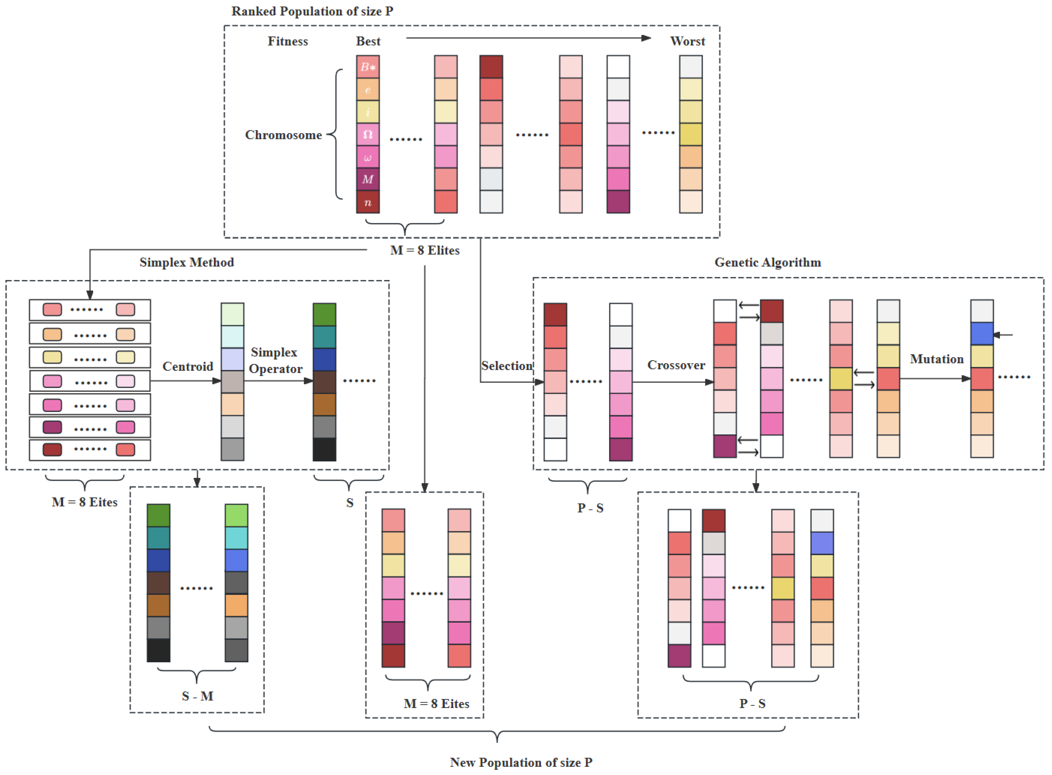
2. SMGA Method
2.1. Genetic Algorithm
2.2. Simplex Method
2.3. SMGA
| Algorithm 1: SMGA |
| input: , |
| output: the best chromosome |
| 1 Initialize a random population of size . 2 While (a terminal condition is not met) 3 { 4 Evaluate the fitness of each chromosome; 5 Rank population based on the fitness results; 6 Copy 8 best chromosomes to the next generation; 7 ******Simplex Part****** 8 Apply simplex operator to the top 8 chromosomes and generate − 8 chromosomes; 9 Copy the generated − 8 chromosomes to the next generation; 10 ****** GA Operator Part****** 11 Select − chromosomes based on ranking, and copy to the next generation; 12 Apply mutation with the mutation probability to the − chromosomes; 13 Apply two parents crossover with the crossover probability to the − chromosomes; 14 } |
3. Settings of the SMGA Parameters
3.1. The Estimation of the Convergence Radius
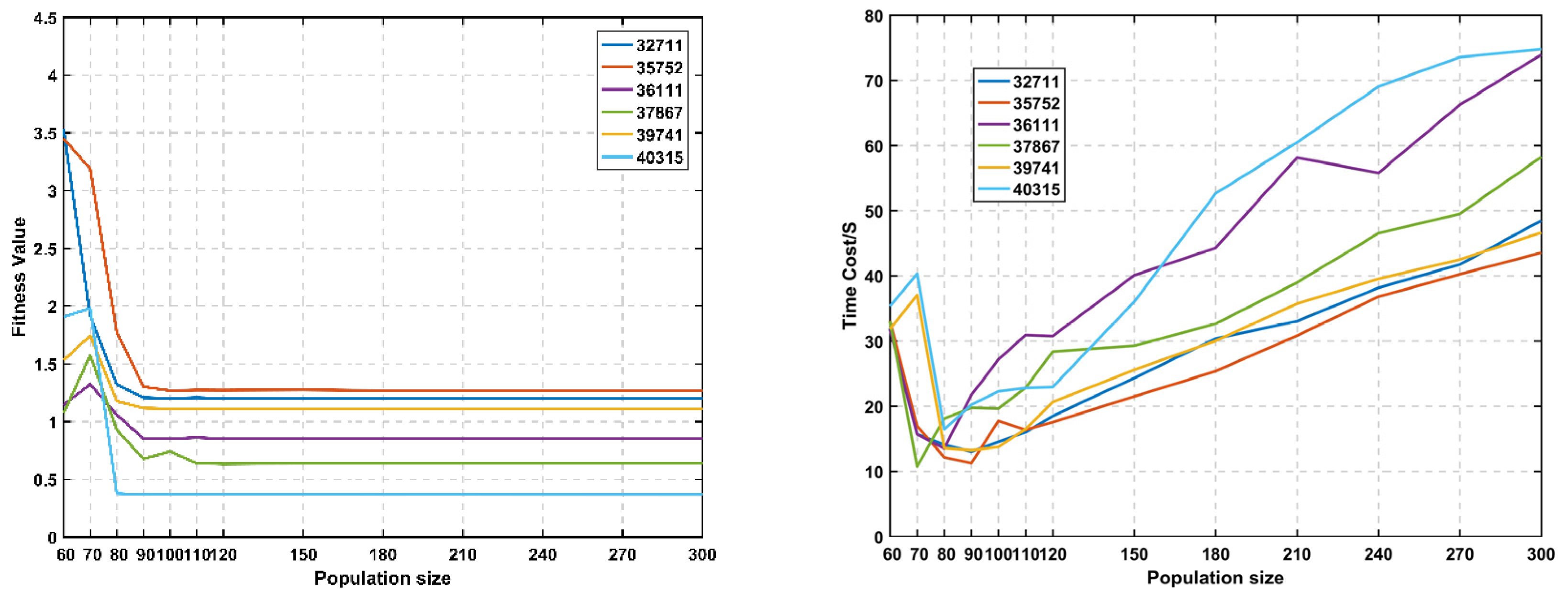
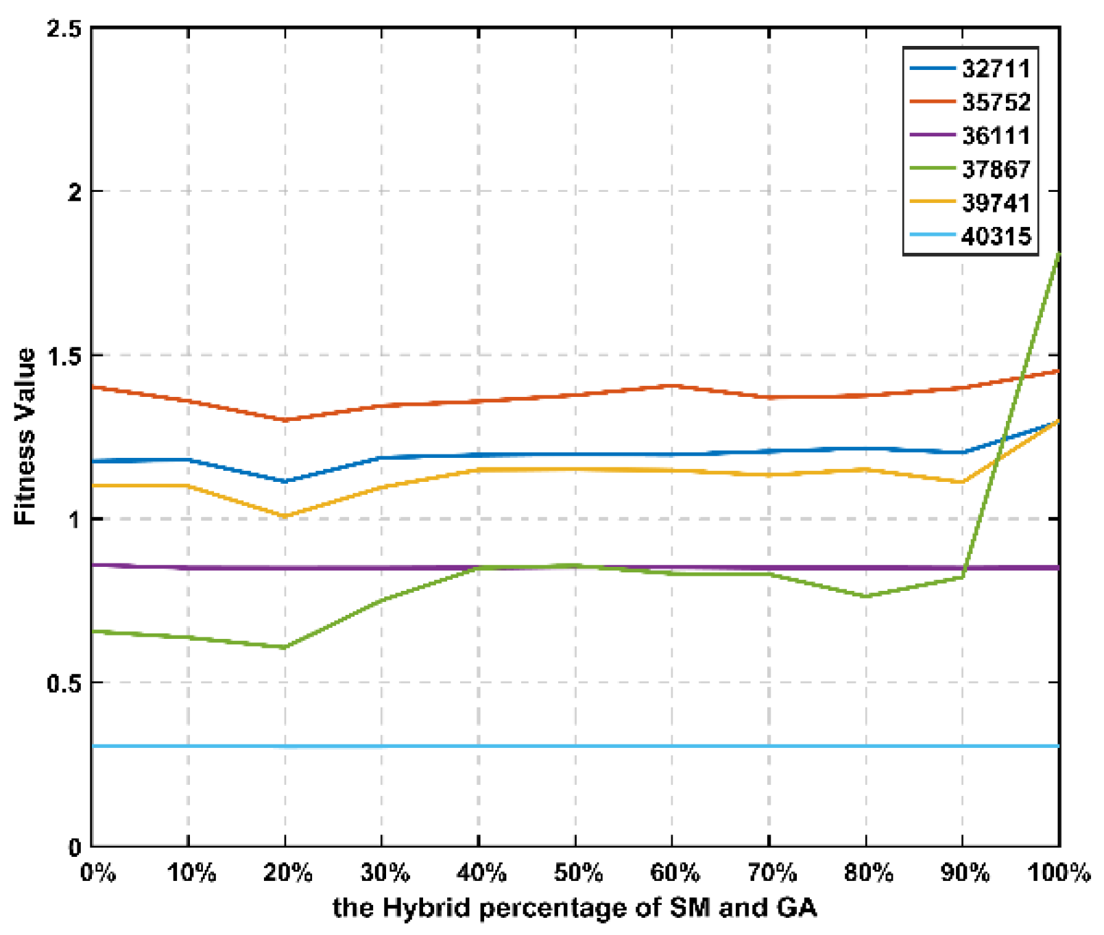
3.2. Population Size and Hybrid Percentage
4. Performance of the SMGA
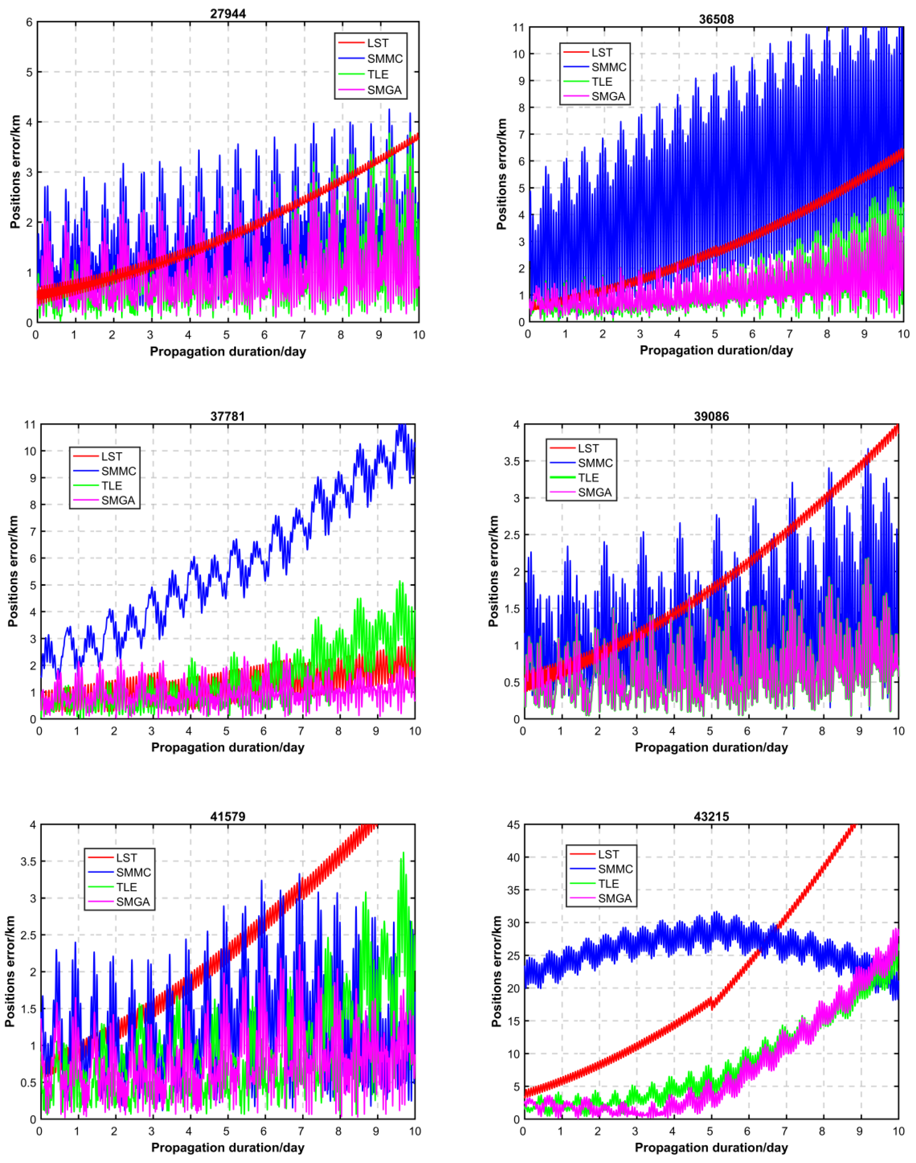
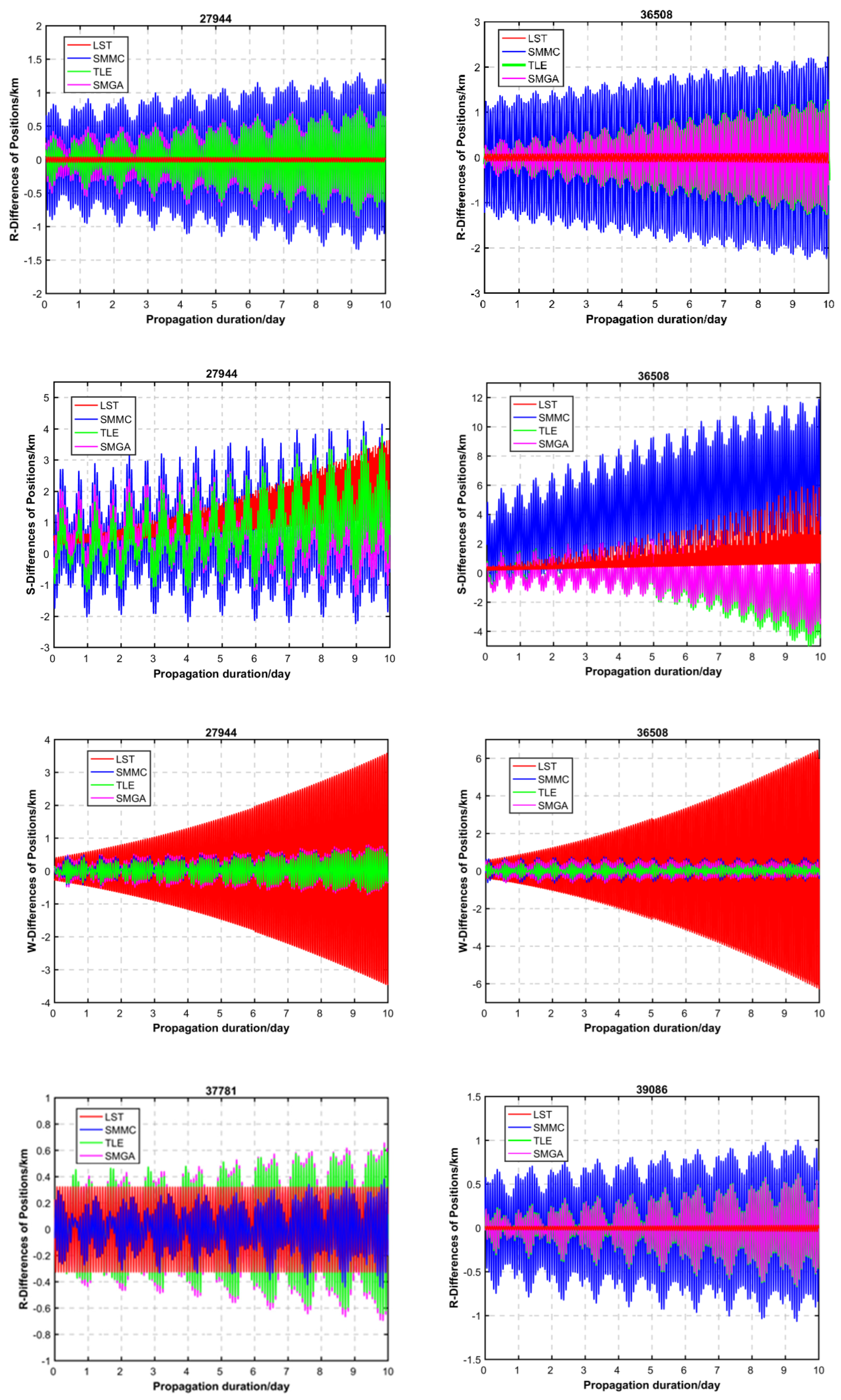
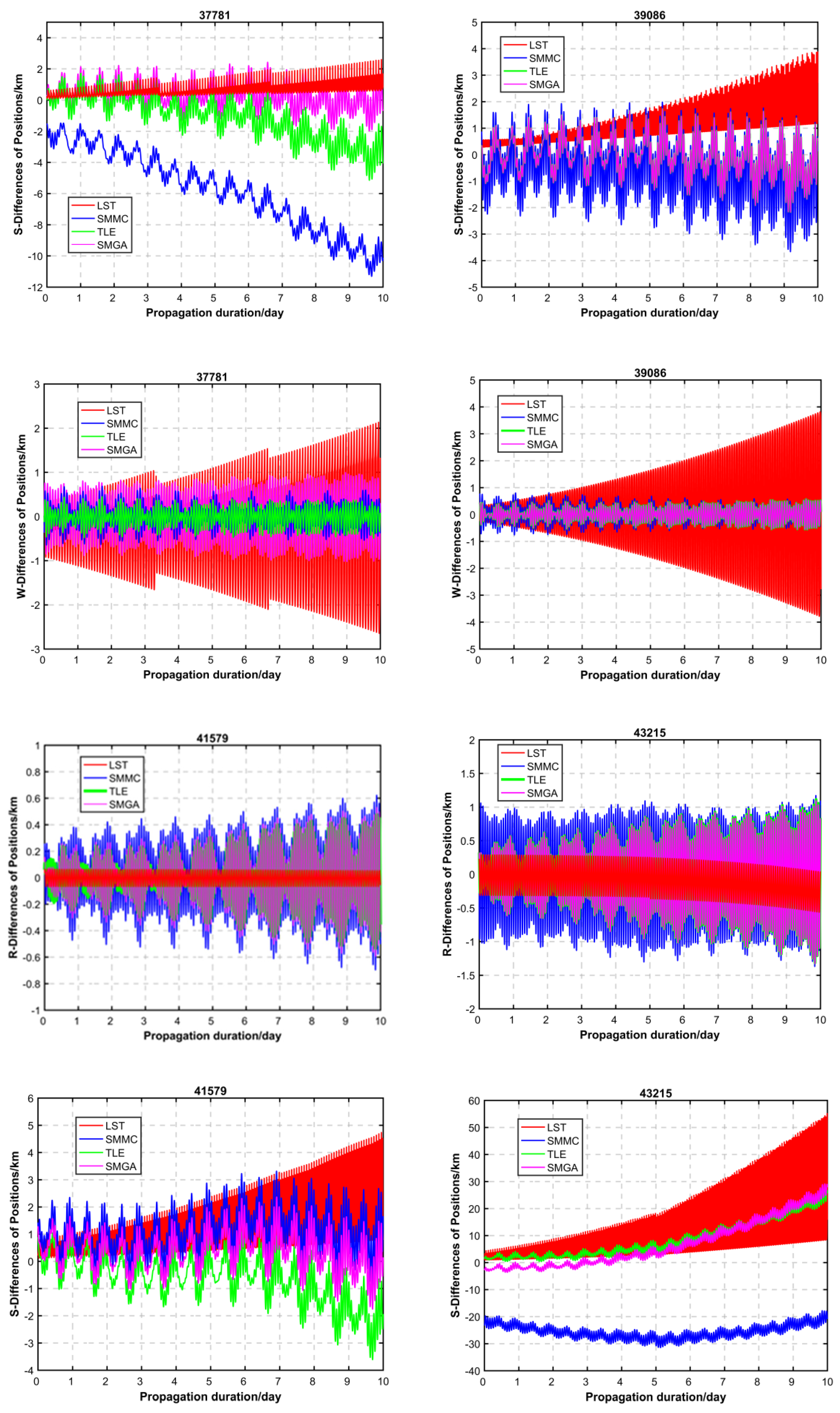
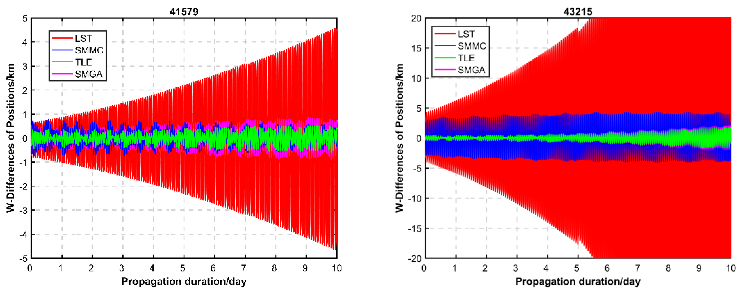
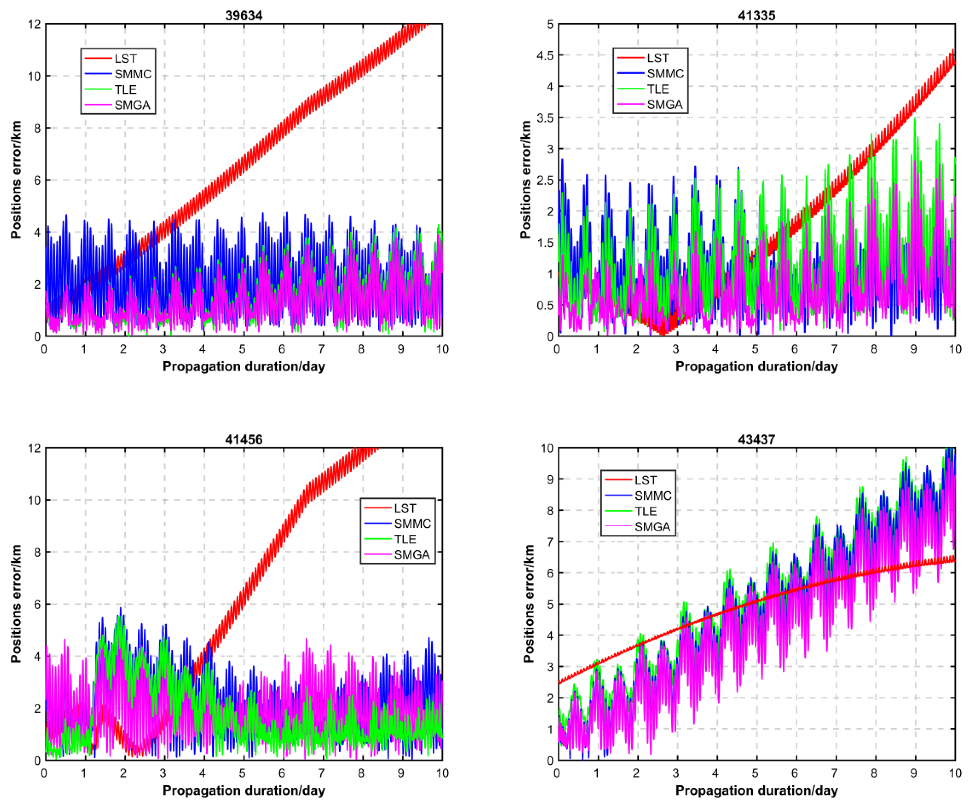
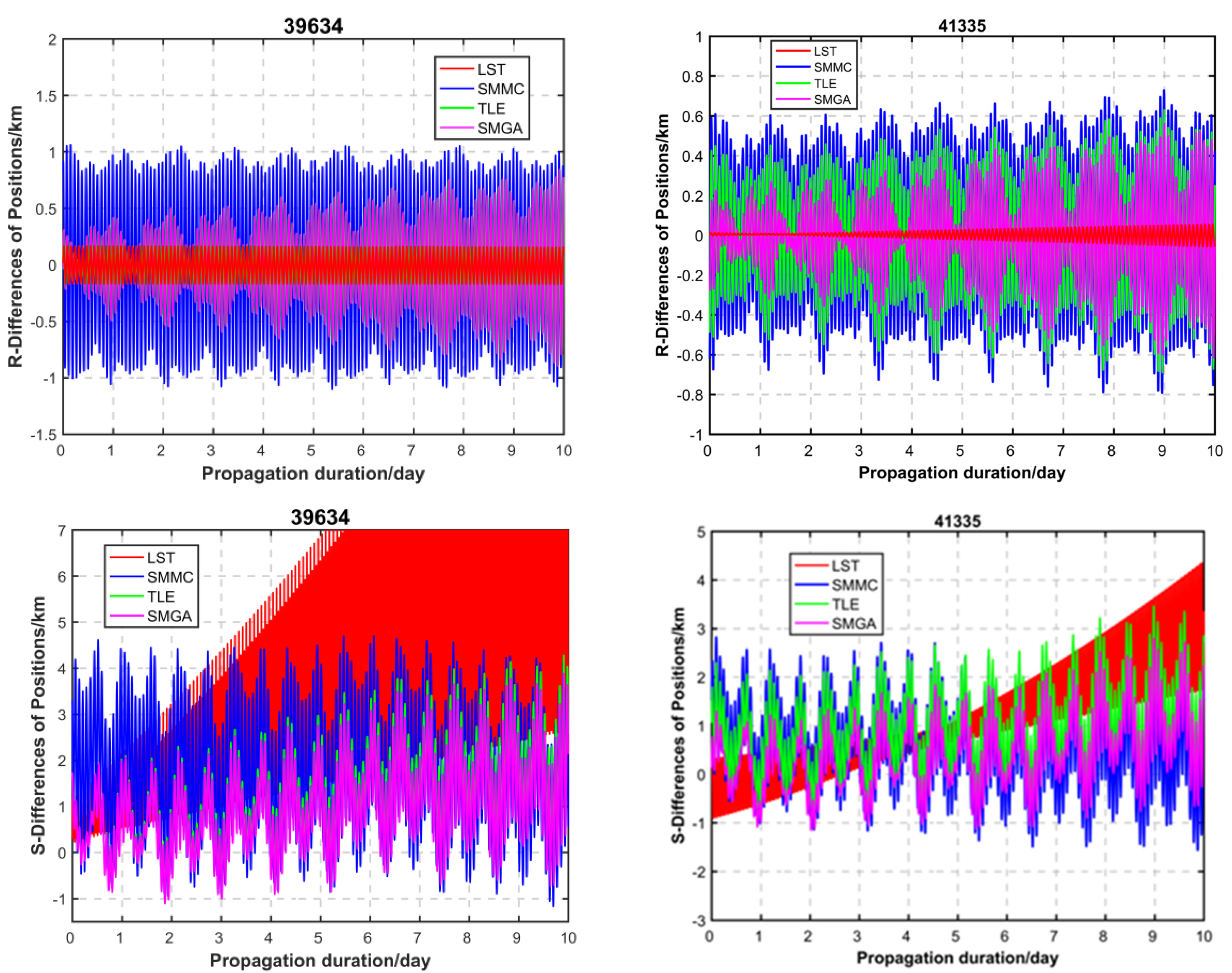
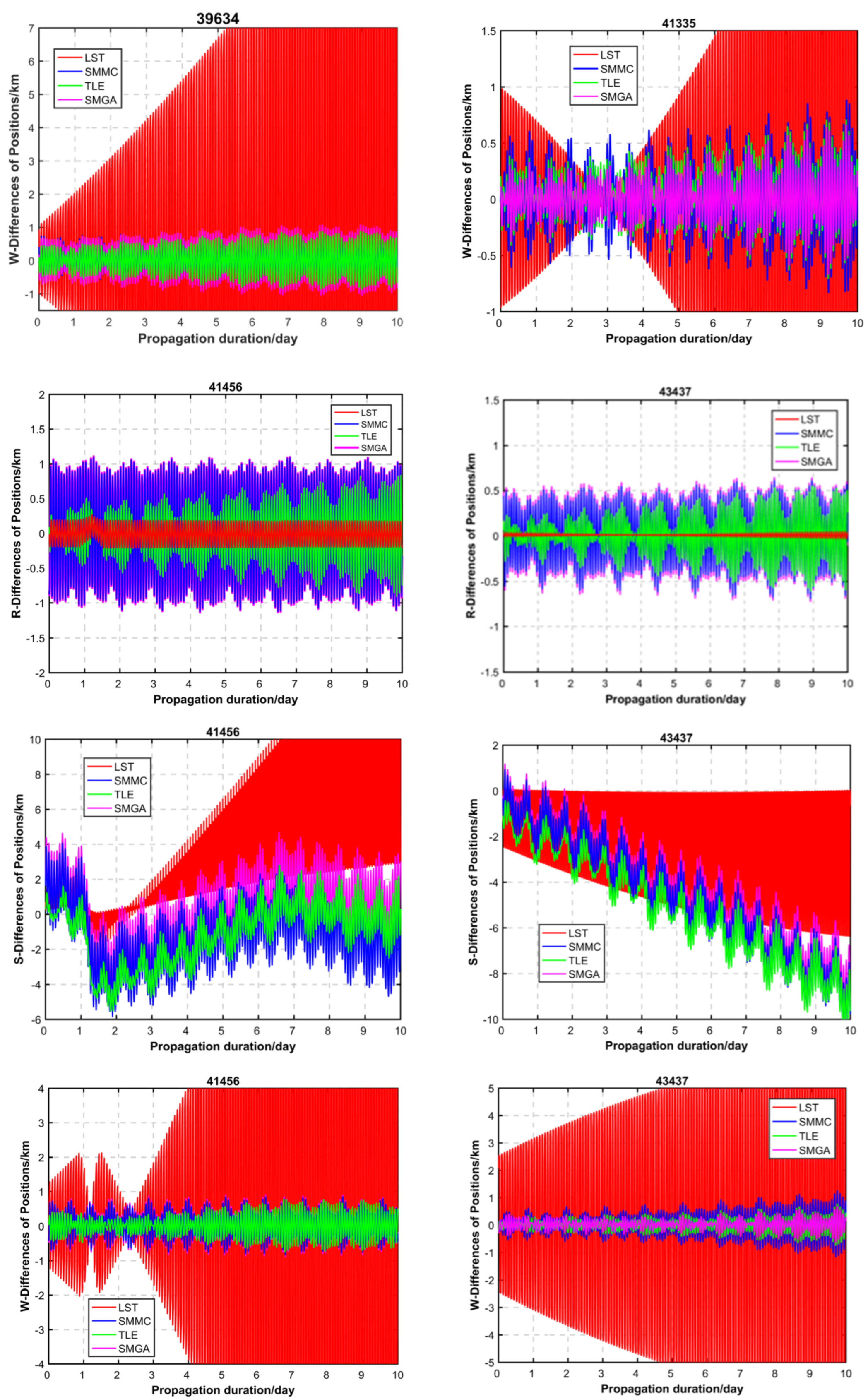
4.1. Performance Evaluation by CPF Data
4.2. Performance Evaluation by POD
4.3. Time Efficiency
5. Conclusions
Author Contributions
Funding
Data Availability Statement
Conflicts of Interest
Appendix A

| NORAD ID | B* | n/rev/day | |||||
|---|---|---|---|---|---|---|---|
| 27944 | 2.3659 × 10⁻⁶ | 1.2406 × 10⁻³ | 98.0084 | 192.5226 | 172.8068 | 187.3303 | 14.63166185 |
| 2.3570 × 10⁻⁶ | 1.1743 × 10⁻³ | 98.0088 | 192.5234 | 171.8911 | 188.2481 | 14.63166104 | |
| −1.3707 × 10⁻⁶ | 1.2469 × 10⁻³ | 98.0083 | 192.5237 | 171.7547 | 188.3863 | 14.63166162 | |
| 36508 | 1.5862 × 10⁻⁵ | 7.3714 × 10⁻⁴ | 92.0234 | 264.1341 | 174.5204 | 185.6129 | 14.52178316 |
| 85944 × 10−6 | 5.9500 × 10⁻⁴ | 92.0252 | 264.1371 | 173.7191 | 186.4005 | 14.52177281 | |
| 2.0176 × 10⁻⁵ | 7.4312 × 10⁻⁴ | 92.0233 | 264.1365 | 173.2464 | 186.8845 | 14.52178378 | |
| 37781 | 2.5213 × 10⁻⁵ | 1.8491 × 10⁻⁴ | 99.3280 | 70.2115 | 64.8181 | 295.3147 | 13.78718375 |
| 7.2779 × 10⁻⁵ | 1.3472 × 10⁻⁴ | 99.3297 | 70.2138 | 69.0775 | 291.0673 | 13.78719592 | |
| 8.3012 × 10⁻⁵ | 1.8802 × 10⁻⁴ | 99.3277 | 70.2150 | 69.1368 | 290.9974 | 13.78718417 | |
| 39086 | 1.1276 × 10⁻⁵ | 1.0252 × 10⁻⁴ | 98.5392 | 247.4978 | 152.6181 | 207.5057 | 14.32008897 |
| 1.4513 × 10⁻⁵ | 3.8322 × 10⁻⁵ | 98.5418 | 247.4977 | 152.6171 | 207.5085 | 14.32009036 | |
| 1.6888 × 10⁻⁵ | 1.0252 × 10⁻⁴ | 98.5392 | 247.4978 | 152.6181 | 207.5057 | 14.32008897 | |
| 41579 | −4.0351 × 10⁻⁵ | 9.2643 × 10⁻⁵ | 99.2713 | 71.1293 | 91.4909 | 268.6396 | 13.85914085 |
| 3.3490 × 10⁻⁵ | 6.3267 × 10⁻⁵ | 99.2314 | 61.0586 | 124.2596 | 235.8607 | 13.85892739 | |
| 3.0056 × 10⁻⁵ | 9.2534 × 10⁻⁵ | 99.2713 | 71.1325 | 93.7722 | 266.3539 | 13.85914052 | |
| 43215 | 4.8931 × 10⁻⁷ | 1.6322 × 10⁻⁴ | 97.4461 | 309.1859 | 78.9253 | 14.5184 | 15.19150418 |
| 5.7057 × 10⁻⁶ | 1.6764 × 10⁻⁴ | 97.4462 | 309.1859 | 78.9253 | 14.5184 | 15.19150418 | |
| 5.7057 × 10⁻⁷ | 1.6762 × 10⁻⁴ | 97.4462 | 309.1859 | 78.9253 | 14.5184 | 15.19150418 |
| NORAD ID | B* | n/rev/day | |||||
|---|---|---|---|---|---|---|---|
| 39634 | 1.4234 × 10⁻⁶ | 1.3067 × 10⁻⁴ | 98.1820 | 279.0364 | 79.6806 | 280.5522 | 14.59198210 |
| 5.1419 × 10⁻⁶ | 7.0174 × 10⁻⁶ | 98.1842 | 279.0378 | 79.4074 | 280.7134 | 14.59198458 | |
| 2.1322 × 10⁻⁶ | 1.3047 × 10⁻⁴ | 98.1819 | 279.0383 | 79.6143 | 280.5203 | 14.59198175 | |
| 41335 | 1.4130 × 10⁻⁵ | 8.6351 × 10⁻⁵ | 98.6304 | 338.8417 | 106.1387 | 253.9889 | 14.26735318 |
| 1.3920 × 10⁻⁵ | 4.7154 × 10⁻⁵ | 98.6304 | 338.8413 | 106.1272 | 253.9958 | 14.26735330 | |
| 1.4130 × 10⁻⁵ | 8.6324 × 10⁻⁵ | 98.6304 | 338.8417 | 106.1387 | 253.9889 | 14.26735318 | |
| 41456 | 5.6384 × 10⁻⁶ | 1.3200 × 10⁻⁴ | 98.1863 | 278.8303 | 79.6261 | 280.4932 | 14.59198565 |
| 1.1364 × 10⁻⁵ | 4.4432 × 10⁻⁶ | 98.1858 | 278.8298 | 78.5882 | 281.5333 | 14.59198870 | |
| 5.5604 × 10⁻⁶ | 1.3384 × 10⁻⁴ | 98.1819 | 278.8297 | 78.5893 | 281.5450 | 14.59198462 | |
| 43437 | 2.1340 × 10⁻⁵ | 7.1593 × 10⁻⁵ | 98.6198 | 338.4481 | 99.6473 | 260.4783 | 14.26740698 |
| 2.5097 × 10⁻⁵ | 2.1841 × 10⁻⁵ | 98.6221 | 338.4496 | 102.5979 | 257.5227 | 14.26740729 | |
| 2.1642 × 10⁻⁵ | 7.2241 × 10⁻⁵ | 98.6198 | 338.4494 | 99.6961 | 260.4301 | 14.26740702 |
References
- Thammawichai, M.; Luangwilai, T. Data-driven satellite orbit prediction using two-line elements. Astron. Comput. 2024, 46, 100782. [Google Scholar] [CrossRef]
- ESA’s Space Debirs Office, Space Debris by the Numbers. 2025. Available online: https://www.esa.int/Space_Safety/Space_Debris/Space_debris_by_the_numbers (accessed on 31 March 2025).
- Saksha, N.O.; Shivarajaiah, A.; Ali, T.; Vaz, A.; Yadav, M.; Hegde, N. Space Situational Awareness: Conjunction-based Collision Analysis Among Debris and Active Assets in Space. Res. Sq. 2024. [CrossRef]
- Gondelach, D.J.; Armellin, R.; Lidtke, A.A. Ballistic coefficient estimation for reentry prediction of rocket bodies in eccentric orbits based on TLE data. Math. Probl. Eng. 2017, 2017, 7309637. [Google Scholar] [CrossRef]
- Abdelaziz, A.M.; Ibrahim, M.; Liang, Z.; Dong, X.; Tealib, S.K. Orbit Predictions for Space Object Tracked by Ground-Based Optical and SLR Stations. Remote Sens. 2022, 14, 4493. [Google Scholar] [CrossRef]
- Doornbos, E.; Klinkrad, H.; Visser, P. Use of two-line element data for thermosphere neutral density model calibration. Adv. Space Res. 2008, 41, 1115–1122. [Google Scholar] [CrossRef]
- Lin, C.; Junyu, C. Using long short-term memory neural network for satellite orbit prediction based on two-line element data. IEEE Trans. Aerosp. Electron. Syst. 2025. [Google Scholar] [CrossRef]
- Roberts, T.G.; Linares, R. Satellite repositioning maneuver detection in geosynchronous orbit using two-line element (TLE) data. In Proceedings of the 71st International Astronautical Congress, Dubai, United Arab Emirates, 12–16 October 2020. [Google Scholar]
- Anselmo, L.; Pardini, C. Analysis of the consequences in low Earth orbit of the collision between Cosmos 2251 and Iridium 33. In Proceedings of the 21st International Symposium on Space Flight Dynamics, Toulouse, France, 28 September–2 October 2009; Centre Nationale D’etudes Spatiales: Paris, France, 2009. [Google Scholar]
- Paulet, T.; Cazabonne, B. An open-source solution for TLE based Orbit Determination. In Proceedings of the 8th European Conference on Space Debris, Darmstadt, Germany, 20–23 April 2021. [Google Scholar]
- Lidtke, A.A.; Gondelach, D.J.; Armellin, R. Optimising filtering of two-line element sets to increase re-entry prediction accuracy for GTO objects. Adv. Space Res. 2019, 63, 1289–1317. [Google Scholar] [CrossRef]
- Vallado, D.; Crawford, P. SGP4 orbit determination. In Proceedings of the AIAA/AAS Astrodynamics Specialist Conference and Exhibit, Monterey, CA, USA, 5–8 August 2008. [Google Scholar]
- Racelis, D.; Joerger, M. High-integrity TLE error models for MEO and GEO satellites. In Proceedings of the 2018 AIAA SPACE and Astronautics Forum and Exposition, Orlando, FL, USA, 17–19 September 2018. [Google Scholar]
- Riesing, K. Orbit determination from two line element sets of ISS-deployed cubesats. In Proceedings of the 29th Annual AIAA/USU Conference on Small Satellites, Logan, UT, USA, 8–13 August 2015. [Google Scholar]
- Kazemi, S.; Azad, N.L.; Scott, K.A.; Oqab, H.B.; Dietrich, G.B. Orbit determination for space situational awareness: A survey. Acta Astronaut. 2024, 2024, 272–295. [Google Scholar] [CrossRef]
- Levit, C.; Marshall, W. Improved orbit predictions using two-line elements. Adv. Space Res. 2011, 47, 1107–1115. [Google Scholar] [CrossRef]
- Águeda, A.; Aivar, L.; Tirado, J.; Dolado, J.C. In-orbit lifetime prediction for LEO and HEO based on orbit determination from TLE data. In Proceedings of the 6th European Conference on Space Debris, Darmstadt, Germany, 22–25 April 2013. [Google Scholar]
- Dudek, N. Improved Orbit Determination and Prediction of Delfi-PQ Satellite Using Two-Line Elements. Bachelor’s Thesis, Delft University of Technology, Delft, The Netherlands, 2024; pp. 1–8. [Google Scholar]
- Hallgarten La Casta, M.I.; Amato, D. Debiasing of two-line element sets for batch least squares pseudo-orbit determination in MEO and GEO. arXiv 2024, arXiv:2412.15793v1. [Google Scholar] [CrossRef]
- Goh, S.T.; Low, K.S. Real-time estimation of satellite’s two-line elements via positioning data. In Proceedings of the 2018 IEEE Aerospace Conference, Big Sky, MT, USA, 3–10 March 2018. [Google Scholar]
- Jamali, S.E.; Masud, M.M. Orbit propagation and determination using genetic algorithms. In Proceedings of the 2023 15th International Conference on Innovations in Information Technology (IIT), Al Ain, United Arab Emirates, 14–15 November 2023. [Google Scholar]
- Liu, J.; Long, W.; Wu, Y.; Xu, J.; Sang, J.; Lei, X. TLE orbit determination using simplex method. Geod. Geodyn. 2023, 14, 438–455. [Google Scholar] [CrossRef]
- Li, B.; Zhang, Y.; Huang, J.; Sang, J. Improved orbit predictions using two-line elements through error pattern mining and transferring. Acta Astronaut. 2021, 188, 405–415. [Google Scholar] [CrossRef]
- Bizalion, H.; Guillot, A.; Petit, A.; Lucken, R. Systematic TLE data improvement by neural network for most cataloged resident space objects. Adv. Space Res. 2023, 72, 2649–2659. [Google Scholar] [CrossRef]
- Subramanian, S.; Ramnani, R.; Sengupta, S.; Yadav, S. Orbit propagation from historical data using physics-informed neural odes. In Proceedings of the 2023 International Conference on Machine Learning and Applications (ICMLA), Jacksonville, FL, USA, 15–17 December 2023. [Google Scholar]
- Jung, O.; Seong, J.; Jung, Y.; Bang, H. Recurrent neural network model to predict re-entry trajectories of uncontrolled space objects. Adv. Space Res. 2021, 68, 2515–2529. [Google Scholar] [CrossRef]
- Clark, N.L. Reduced-Order Atmospheric Density Modeling for LEO Satellite Orbital Reentry Prediction; Massachusetts Institute of Technology: Cambridge, MA, USA, 2023. [Google Scholar]
- Yen, J.; Liao, J.C.; Lee, B.; Randolph, D. A hybrid approach to modeling metabolic systems using a genetic algorithm and simplex method. IEEE Trans. Syst. Man Cybern. Part B 1998, 28, 173–191. [Google Scholar] [CrossRef] [PubMed]
- Haldurai, L.; Madhubala, T.; Rajalakshmi, R. A study on genetic algorithm and its applications. Int. J. Comput. Sci. Eng. 2016, 4, 139–143. [Google Scholar]
- Ren, Z.; San, Y. A hybrid optimized algorithm based on simplex method and genetic algorithm. In Proceedings of the 2006 6th World Congress on Intelligent Control and Automation, Dalian, China, 21–23 June 2006. [Google Scholar]
- Abay, R.; Balage, S.; Brown, M.; Boyce, R. Two-line element estimation using machine learning. J. Astronaut. Sci. 2021, 68, 273–299. [Google Scholar] [CrossRef]
- Liu, J.; Liu, L.; Du, J.; Sang, J. TLE outlier detection based on expectation maximization algorithm. Adv. Space Res. 2021, 68, 2695–2712. [Google Scholar] [CrossRef]
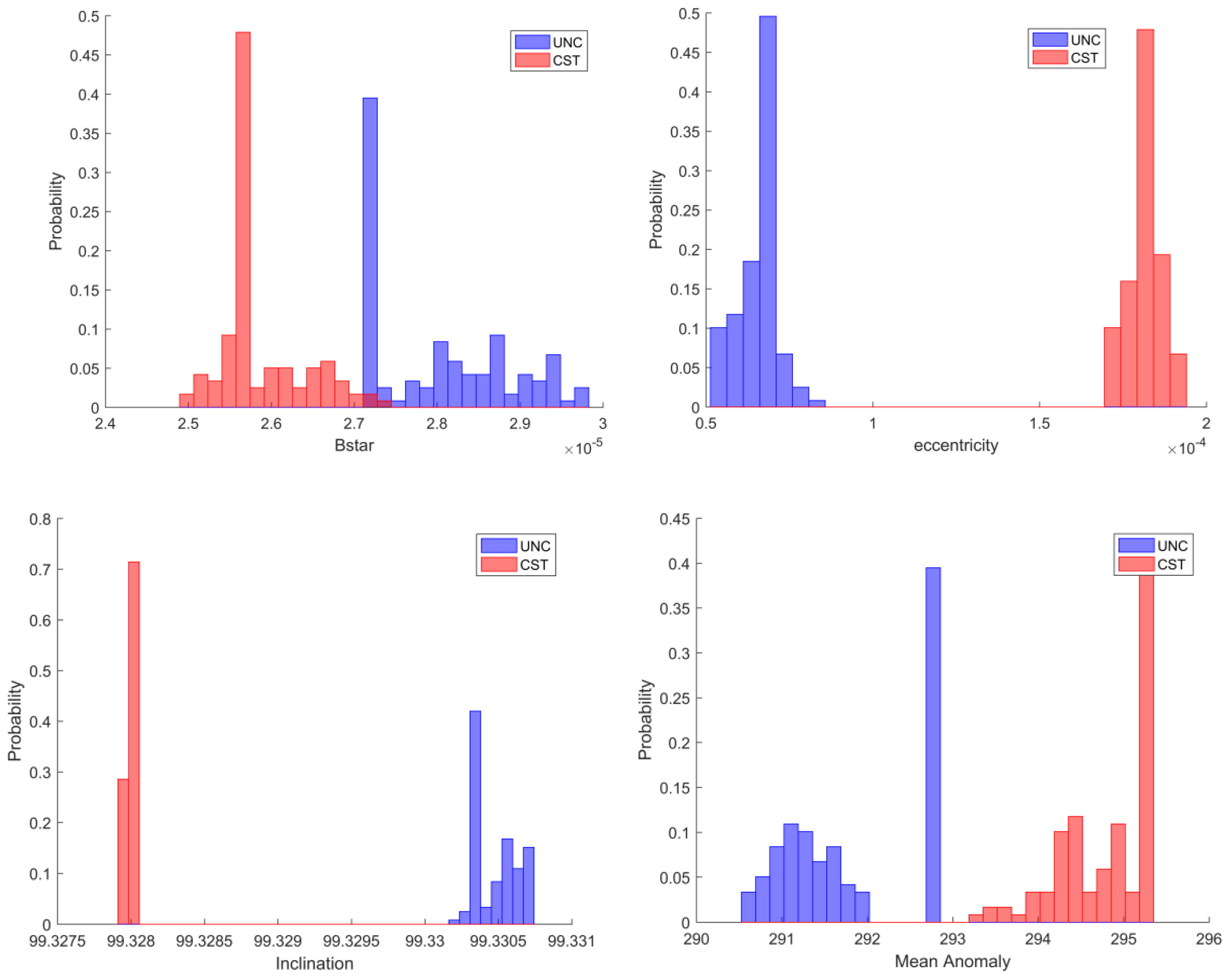
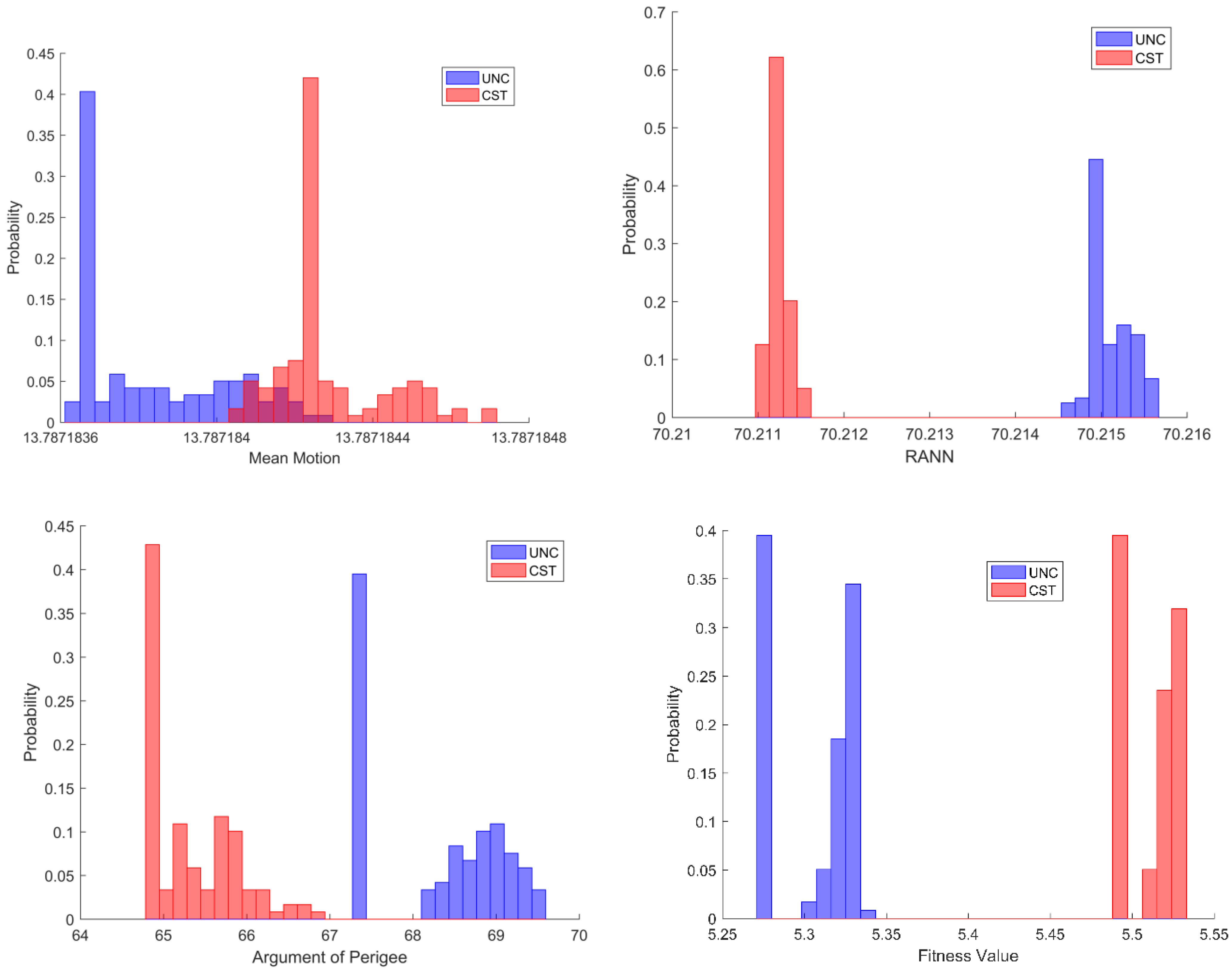
| Epoch | B*/ER | /° | /° | /° | /° | /rev/day | |
|---|---|---|---|---|---|---|---|
| 57.0750 | 1.8160 × 10⁻⁴ | 1.9360 × 10⁻⁴ | 99.3282 | 69.0729 | 75.8652 | 284.2805 | 13.78718758 |
| 57.3653 | −4.8704 × 10⁻⁴ | 1.9080 × 10⁻⁴ | 99.3283 | 69.3581 | 77.2623 | 282.8759 | 13.78718135 |
| 57.5830 | 1.3400 × 10⁻⁴ | 1.9120 × 10⁻⁴ | 99.3284 | 69.5728 | 76.2074 | 283.9263 | 13.78717890 |
| 57.9458 | 4.0391 × 10⁻⁴ | 1.9420 × 10⁻⁴ | 99.3283 | 69.9290 | 68.8161 | 291.3207 | 13.78717853 |
| 58.0910 | 7.7336 × 10⁻⁴ | 1.9000 × 10⁻⁴ | 99.3280 | 70.0726 | 70.3828 | 289.7571 | 13.78719342 |
| 58.2361 | 8.3012 × 10⁻⁵ | 1.8800 × 10⁻⁴ | 99.3277 | 70.2150 | 69.1368 | 290.9974 | 13.78718417 |
| UNC | 2.8012 × 10⁻⁵ | 6.5100 × 10⁻⁴ | 99.3304 | 70.2150 | 68.2390 | 291.8796 | 13.78718383 |
| CST | 2.6804 × 10⁻⁴ | 1.8200 × 10⁻⁴ | 99.3277 | 70.2110 | 64.9200 | 295.2117 | 13.78718425 |
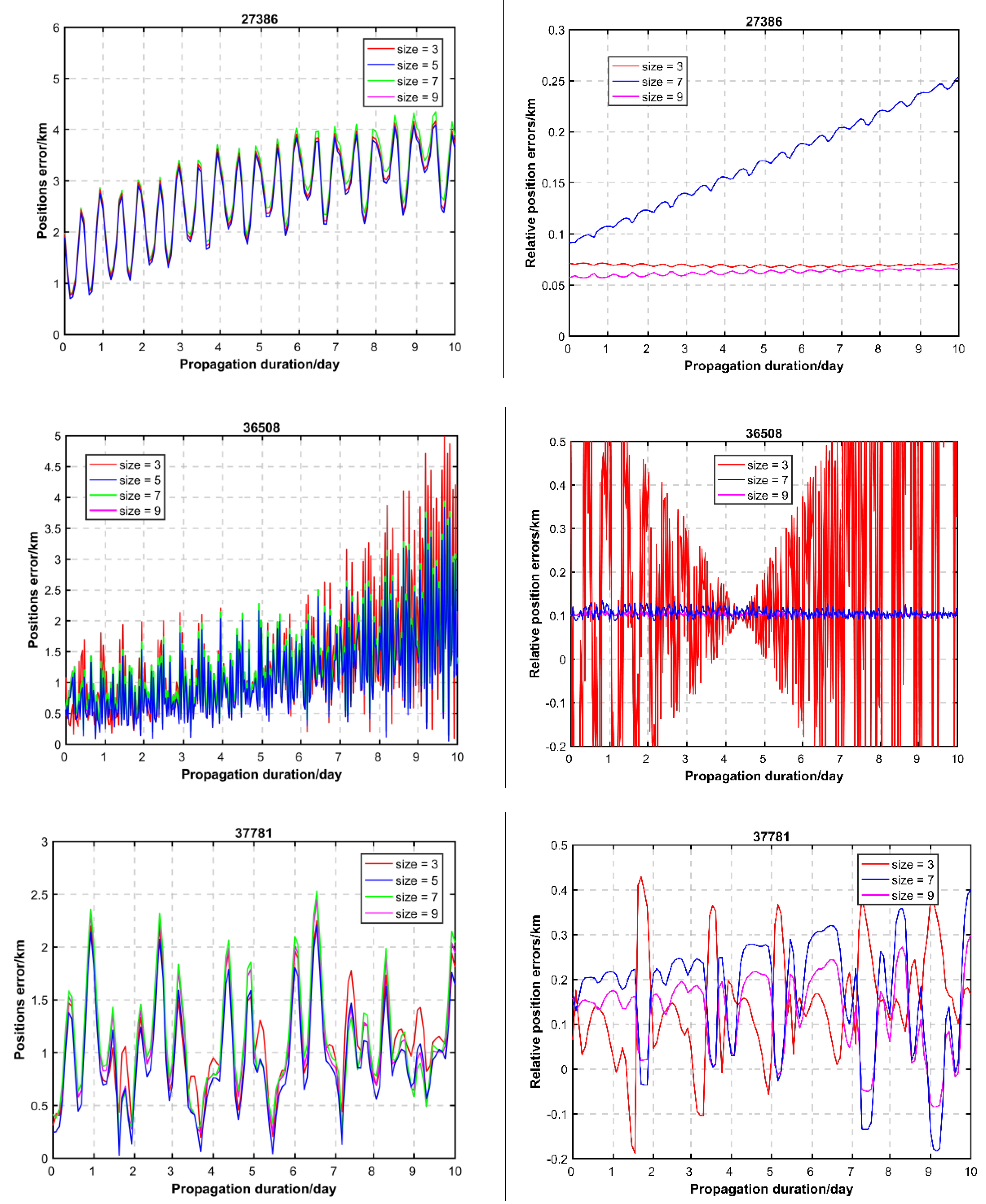
| NORAD ID | Size | ||||
|---|---|---|---|---|---|
| 3 | 5 | 7 | 9 | ||
| 27386 | Error | 8.124 | 8.121 | 8.128 | 8.125 |
| Fitness | 2.392 | 2.400 | 2.500 | 2.400 | |
| 36508 | Error | 14.159 | 11.193 | 11.198 | 11.188 |
| Fitness | 1.344 | 1.213 | 1.220 | 1.216 | |
| 37781 | Error | 6.129 | 6.021 | 6.003 | 5.948 |
| Fitness | 1.064 | 1.029 | 1.098 | 1.055 | |
| Norad ID | Satellite Name | Apogee/km | Perigee/km | |
|---|---|---|---|---|
| 27944 | Larers | 689 | 673 | 98.00 |
| 32711 | NavStar 62 | 20,706 | 19,659 | 54.97 |
| 35752 | NavStar 64 | 20,329 | 20,038 | 54.28 |
| 36111 | SL-4 Deb | 251 | 243 | 64.18 |
| 36508 | CryoSat 2 | 721 | 718 | 92.02 |
| 37781 | Haiyang 2A | 969 | 967 | 99.32 |
| 37867 | Cosmos 2476 | 19,192 | 19,068 | 64.48 |
| 39086 | Saral | 785 | 781 | 98.53 |
| 39634 | Sentinel 1A | 697 | 695 | 98.18 |
| 39741 | NavStar 70 | 20,277 | 20,085 | 55.58 |
| 40315 | Cosmos 2501 | 19,182 | 19,077 | 64.27 |
| 41335 | Sentinel 3A | 803 | 802 | 98.62 |
| 41456 | Sentinel 1B | 492 | 567 | 98.18 |
| 41579 | Cosmos 2517 | 944 | 942 | 99.27 |
| 43215 | PAZ | 510 | 507 | 97.44 |
| 43437 | Sentinel 3B | 804 | 801 | 98.62 |
| NORAD ID | Original TLE/km | LST/km | SMMC/km | SMGA/km | Against Error RMSs with Original TLE in % | ||
|---|---|---|---|---|---|---|---|
| LST | SMMC | SMGA | |||||
| 27944 | 1.237 | 2.065 | 1.710 | 1.202 | 66.94 | 38.24 | 2.83 |
| 36508 | 1.562 | 3.335 | 5.643 | 1.411 | 113.51 | 261.27 | 9.67 |
| 37781 | 1.816 | 1.389 | 6.297 | 1.085 | 23.51 | 246.75 | 40.25 |
| 39086 | 0.786 | 2.167 | 1.435 | 0.784 | 175.70 | 82.57 | 0.25 |
| 41579 | 1.134 | 2.655 | 1.402 | 0.910 | 134.13 | 23.63 | 19.75 |
| 43215 | 10.979 | 27.093 | 25.852 | 10.885 | 146.77 | 135.47 | 0.85 |
| NORAD ID | Original TLE/km | LST/km | SMMC/km | SMGA/km | Against Error RMSs with Original TLE in % | ||
|---|---|---|---|---|---|---|---|
| LST | SMMC | SMGA | |||||
| 39634 | 1.675 | 7.531 | 2.441 | 1.528 | 349.61 | 45.73 | 8.77 |
| 41335 | 1.324 | 2.110 | 1.226 | 0.888 | 59.37 | 7.40 | 32.93 |
| 41456 | 2.140 | 8.154 | 2.203 | 2.073 | 281.03 | 2.94 | 3.13 |
| 43437 | 5.660 | 5.009 | 5.257 | 4.835 | 11.50 | 7.12 | 14.58 |
| NORAD ID | 32711 | 35752 | 36111 | 37867 | 39741 | 40315 | |
|---|---|---|---|---|---|---|---|
| SMGA | Fitness | 1.214 | 1.265 | 1.113 | 0.848 | 0.636 | 0.365 |
| Time/s | 14.521 | 17.754 | 27.272 | 19.644 | 13.238 | 22.272 | |
| SMMC | Fitness | 1.672 | 1.586 | 1.443 | 1.115 | 0.923 | 0.474 |
| Time/m | 24.619 | 25.773 | 31.576 | 26.222 | 22.041 | 27.311 | |
| LST | Fitness | 1.741 | 1.432 | 1.521 | 1.230 | 1.002 | 0.530 |
| Time/m | 1.363 | 1.417 | 1.833 | 1.413 | 1.210 | 1.658 | |
Disclaimer/Publisher’s Note: The statements, opinions and data contained in all publications are solely those of the individual author(s) and contributor(s) and not of MDPI and/or the editor(s). MDPI and/or the editor(s) disclaim responsibility for any injury to people or property resulting from any ideas, methods, instructions or products referred to in the content. |
© 2025 by the authors. Licensee MDPI, Basel, Switzerland. This article is an open access article distributed under the terms and conditions of the Creative Commons Attribution (CC BY) license (https://creativecommons.org/licenses/by/4.0/).
Share and Cite
Liu, J.; Wu, C.; Long, W.; Yuan, B.; Zhang, Z.; Sang, J. Improving Orbit Prediction of the Two-Line Element with Orbit Determination Using a Hybrid Algorithm of the Simplex Method and Genetic Algorithm. Aerospace 2025, 12, 527. https://doi.org/10.3390/aerospace12060527
Liu J, Wu C, Long W, Yuan B, Zhang Z, Sang J. Improving Orbit Prediction of the Two-Line Element with Orbit Determination Using a Hybrid Algorithm of the Simplex Method and Genetic Algorithm. Aerospace. 2025; 12(6):527. https://doi.org/10.3390/aerospace12060527
Chicago/Turabian StyleLiu, Jinghong, Chenyun Wu, Wanting Long, Bo Yuan, Zhengyuan Zhang, and Jizhang Sang. 2025. "Improving Orbit Prediction of the Two-Line Element with Orbit Determination Using a Hybrid Algorithm of the Simplex Method and Genetic Algorithm" Aerospace 12, no. 6: 527. https://doi.org/10.3390/aerospace12060527
APA StyleLiu, J., Wu, C., Long, W., Yuan, B., Zhang, Z., & Sang, J. (2025). Improving Orbit Prediction of the Two-Line Element with Orbit Determination Using a Hybrid Algorithm of the Simplex Method and Genetic Algorithm. Aerospace, 12(6), 527. https://doi.org/10.3390/aerospace12060527