Optimal Low-Thrust Transfers Between Relative Planar and Spatial Quasi-Satellite Orbits in the Earth–Moon System

Abstract

This paper investigates the design of optimal low-thrust transfers between relative planar and spatial quasi-satellite orbits (QSOs) in the Earth–Moon system under the Circular Restricted Three-Body Problem (CR3BP). A key contribution is the adaptation of a trajectory optimization framework, previously applied to halo orbit transfers, to accommodate the unique challenges of QSO families, especially the transition between planar and spatial configurations. The method employs a refined beam search strategy to construct diverse initial guess chains, which are then optimized via a successive convexification algorithm tailored for the spatial dynamics of QSOs. Additionally, a linear–quadratic regulator (LQR)-based control scheme is implemented to ensure long-term station-keeping of the final 3D-QSO. Simulation results demonstrate the feasibility of connecting planar and spatial QSOs with minimum-fuel trajectories while maintaining bounded terminal deviations, offering new tools for future Earth–Moon logistics and navigation infrastructure. Key findings include the successful design of low-thrust transfer trajectories between planar QSOs and 1:5 3D-QSOs, with a minimum total $\mathsf{\Delta }V$ of 195.576 m/s over a time of flight (ToF) of 261 days, and a minimum ToF of 41 days with a total $\mathsf{\Delta }V$ of 270.507 m/s. Additionally, the application of LQR control demonstrated the ability to maintain 1:5 3D-QSO families around the Moon with less than 12 mm/s $\mathsf{\Delta }V$ over two months. This research provides valuable insights into the optimization of low-thrust transfer trajectories and the application of advanced control techniques for space missions, particularly those targeting lunar and planetary satellite exploration.

1. Introduction

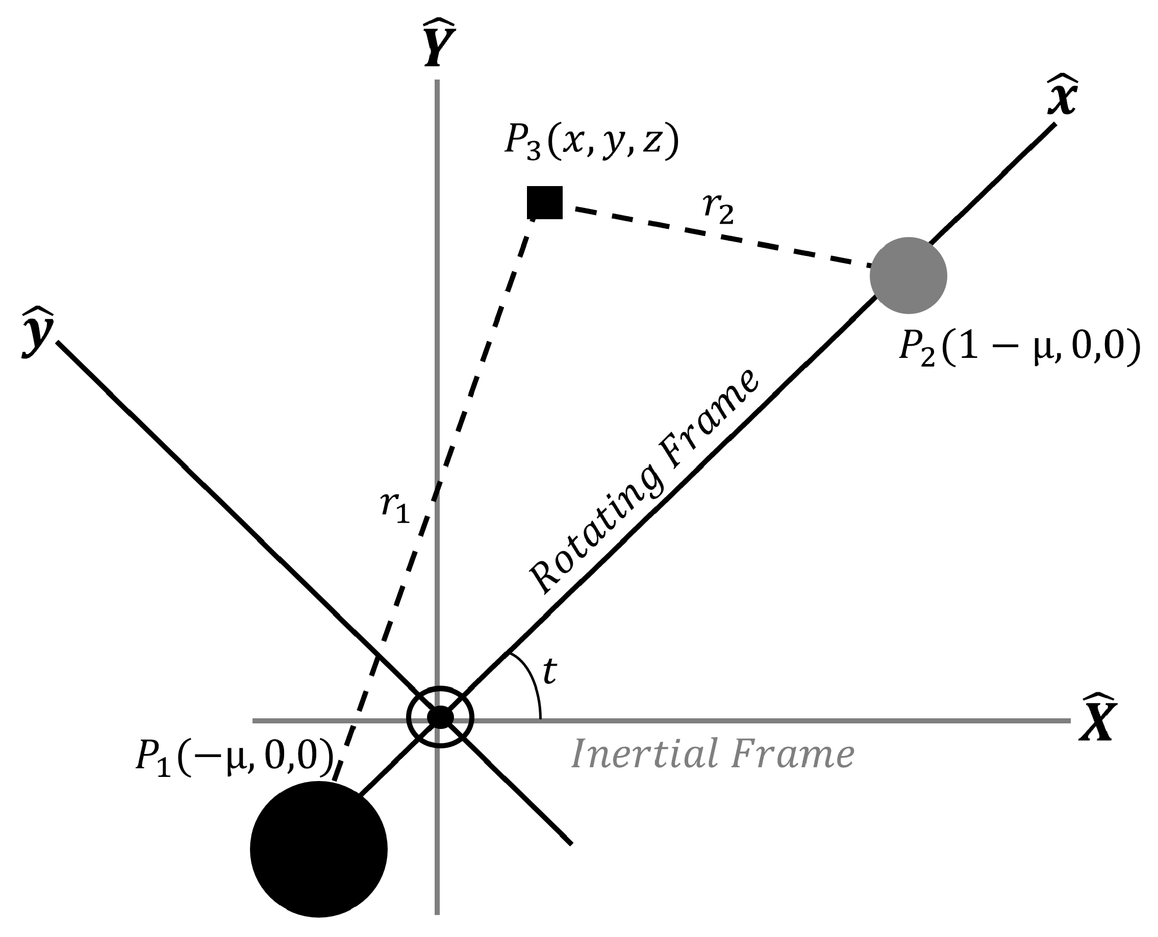
Quasi-satellite orbits are distant retrograde orbits that are often classified as f-family in the literature [1], are usually stable, and have gained attention as potential candidates for the exploration of the Moon and remote planetary satellites in the Circular Restricted Three-Body Problem. Distant retrograde orbits (DROs), are periodic orbits in the rotating frame and appear as large quasi-elliptical retrograde orbits around the secondary body, hence QSOs. QSOs are characterized by their interactions with two Lagrange points ($L_1$ and $L_2$) of the CRTBP, which provide gravitational balance and stability. QSOs have several advantages over other types of orbits, such as low energy requirements, low perturbations, high visibility, and more extended periods [2]. Several mission design proposals have used QSOs or DROs as parking orbits, staging orbits, or communication relay orbits for various purposes, such as scientific exploration, resource utilization, or human settlement [3,4]. A few recent examples include NASA’s Orion spacecraft, which entered a DRO around the Moon during the Artemis 1 mission, becoming the first spacecraft to use this orbit [5]. China’s Chang’e 5 orbiter also entered a DRO around the Moon in 2022 after returning lunar samples to Earth and performing solar observations at another Lagrange point [6]. DROs have been proposed for other missions, such as the Jupiter Icy Moons Orbiter, which would have used a DRO around Europa to study its surface and subsurface ocean [7]. JAXA’s upcoming robotic sample return mission, Martian Moons eXploration (MMX), will use QSO to explore Phobos [8].

Most of these missions use the planar QSO or DRO family and have several mission limitations on using these orbits for scientific imaging of high-latitude regions of the planetary satellites. In this paper, following [9,10,11], we leverage the vertical instability of planar families to identify out-of-plane QSOs that bifurcate from the families of planar QSOs and implement low-thrust transfer strategies to reach these three-dimensional QSOs (3D-QSOs) using a beam-search-aided successive convex optimization method [12]. Specifically, we have used the bifurcated families from the planar QSO families around the Moon in the Earth–Moon CRTBP system. In this paper, firstly, retrograde families of periodic orbits are computed numerically using single shooting and pseudo-arclength continuation methods [13] followed by bifurcation analysis to detect out-of-plane bifurcation points [14,15,16] and used as a first guess for a multiple shooting strategy that generates entire families of spatial retrograde orbits around the Moon [17,18]. Later, we utilize family members as intermediate orbits to connect them with the planar and spatial QSO using a beam search algorithm using successive convex optimization.

Previously, transfers to QSO from Low Earth Orbits using the manifolds of collinear equilibrium point orbits of the Sun–Earth CRTBP have been studied by Scott and Spencer [19], and in the framework of Earth–Moon CRTBP by [20,21,22]. Low-energy transfers from Lyapunov orbits around cis-lunar Lagrangian points to QSO were studied by [23]. Lam [24] studied the stability of QSO, proposing different transfers between different altitude QSOs using either impulsive or low-thrust propulsion. They applied this strategy to the Jupiter–Europa and Jupiter–Ganymede systems, showing examples of low-thrust trajectories from retrograde relative orbits around the two Jovian moons. Later, transfers near Phobos between QSOs in the context of Martian Moon exploration were studied [25,26]. Despite the number of studies that can be found in the literature, the problem of finding and implementing appropriate optimal transfer techniques between relative planar QSOs, planar to 3D-QSOs, and planet-centric orbits to QSOs is still open to debate.

Classical numerical methods for trajectory optimization problems are divided into indirect and direct methods [27,28]. The utilization of convex optimization tools in spacecraft trajectory design is highly advantageous [29]. Despite being categorized as a direct method, these tools enable the finding of optimal solutions for convex optimization problems through efficient polynomial-time algorithms. 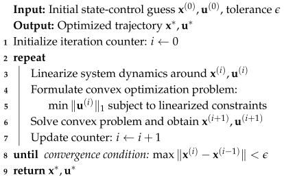Furthermore, any local optimal solution obtained through this technique satisfies the globally optimal condition [30]. In general, trajectory optimization problems exhibit non-convexity as a result of the presence of nonlinear equations of motion. However, this challenge can be solved by applying convexification techniques such as lossless convexification [31,32] and successive convexification [33,34,35,36]. The optimization problem that arises from lossless and successive convexification techniques is commonly referred to as successive convex optimization. This study builds upon the successive convex optimization and beam search strategy previously applied to low-thrust transfers between halo orbits [12,35]. Unlike earlier work, which focused on planar halo dynamics, the present paper tackles a more complex problem involving transfers between quasi-satellite orbits with significant spatial components. The algorithmic framework is adapted to account for the challenges in the QSO regime, including increased dynamical instability, vertical bifurcations, and the need for designing accurate 3D trajectories. This work extends the work of [12] to explore the optimal low-thrust transfer solutions between planar and spatial QSOs. Although the method has proven to provide optimal results for the case of halo–halo transfer, the current work considers periodic orbits with multiplying orbital periods to tackle this transfer problem.

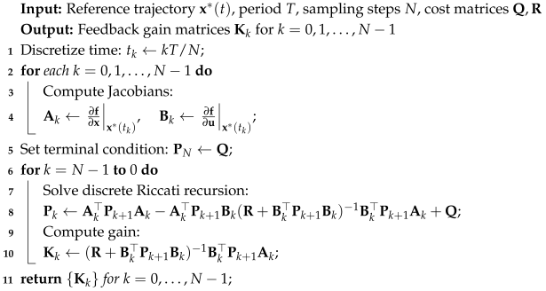
In this research, we have also used the linear quadratic regulator [37,38] of control for station-keeping spacecraft around the Moon. Application of LQR control to spatial periodic orbit families such as 3D-QSOs near the Moon in the Earth–Moon CRTBP framework is also discussed. In this research paper, we apply a commonly used technique for creating feedback control systems based on linear dynamics models, the LQR, to seek and identify the best control inputs by minimizing a quadratic cost function across the states and control inputs of the system. By linearizing the dynamics around a selected reference orbit or point, LQR may be used to stabilize periodic orbits in CRTBP [38]. The linearized model predicts the system’s behavior close to the reference orbit. The system may then be stabilized and regulated around the reference orbit using LQR to construct the control inputs.

Several methods have been explored for designing low-thrust transfers in the CRTBP, including manifold-based connections and direct trajectory optimization. Manifold-based methods exploit the natural dynamics for efficient paths but are typically restricted to impulsive regimes or require precise energy matching. Direct methods offer flexibility but often depend on high-quality initial guesses and may suffer from poor convergence in nonlinear settings. In contrast, our approach integrates beam search for systematic guess generation and successive convexification for robust convergence, offering a practical trade-off between accuracy, generality, and computational cost.

This paper is organized as follows. Section 2 introduces the dynamical model and equations of motion used in this work. Section 3 elaborates on the computation of out-of-plane retrograde orbits around the Moon. Section 4 presents the trajectory optimization used in this research, more explicitly discussing the orbit-chaining process, defining the optimal control problem, and successive convex optimization. Section 5 and Section 6 summarize and apply the transfer methods using beam-search-aided successive convex optimization and application of LQR control of the chosen family of 3D-QSOs with some optimal low-thrust transfer and station-keeping results. Finally, Section 7 provides this research’s summary, key findings, and conclusions.

2. Dynamical Model

The Circular Restricted Three-Body Problem is employed to investigate the motion of a small mass, such as a satellite or spacecraft, subjected to the gravitational fields of two larger masses, typically the Earth and its moon. In the case of the CRTBP Earth–Moon system, the Earth and the Moon are regarded as the primary bodies, while the small mass signifies the satellite or spacecraft. Figure 1 illustrates the schematic of the CRTBP [39,40].

2.1. Linearized Equation

Let $\{x,y,z\}$ be the rotating frame whose origin is the barycenter of the system and $(u_x,u_y,u_z)$ be the control acceleration. Then, the equations of motion of the CRTBP in the non-dimensional form are given by [39,40]

$$\begin{array}{cc}\hfill & \left\{\begin{array}{ccc}\ddot{x}-2\dot{y}& =& {\displaystyle \frac{\partial U}{\partial x}+u_x}\\ \ddot{y}+2\dot{x}& =& {\displaystyle \frac{\partial U}{\partial y}+u_y}\\ \ddot{z}& =& {\displaystyle \frac{\partial U}{\partial z}+u_z}\end{array}\right.\hfill \\ \hfill & U={\displaystyle \frac{1-\mu }{r_1}}+{\displaystyle \frac{\mu }{r_2}}+{\displaystyle \frac{1}{2}}(x^2+y^2)\hfill \\ \hfill & r_1={[{(x+\mu )}^2+y^2+z^2]}^{1/2},\hfill \\ \hfill & r_2={[{(x-1+\mu )}^2+y^2+z^2]}^{1/2}\hfill \end{array}$$

(1)

where $\mu =M_2/(M_1+M_2)$ is the gravitational parameter ($M_1$ and $M_2$ are the masses of the primaries, $M_1>M_2$).

Defining

$\mathbf{x}={\left[\begin{array}{cccccc}x& y& z& \dot{x}& \dot{y}& \dot{z}\end{array}\right]}^T={\left[\begin{array}{cc}\mathit{r}& \mathit{v}\end{array}\right]}^T$ and $\mathbf{u}={\left[\begin{array}{ccc}{u}_x& u_y& u_z\end{array}\right]}^T$, Equation (1) in the state space form becomes

$$\begin{array}{cc}\hfill \dot{\mathit{x}}& =\mathit{f}\left(\mathit{x}\right)+B\mathit{u}=\left[\begin{array}{c}\mathit{v}\\ U_{\mathit{r}}+2\mathsf{\Omega }\mathit{v}\end{array}\right]+\left[\begin{array}{c}{O}_{3\times 3}\\ I_{3\times 3}\end{array}\right]\mathit{u}\hfill \\ \hfill \mathsf{\Omega }& =\left[\begin{array}{ccc}0& 1& 0\\ -1& 0& 0\\ 0& 0& 0\end{array}\right]\hfill \end{array}$$

(2)

where $\mathit{f}\left(\mathbf{x}\right)$ corresponds to the nonlinear part of the CRTBP equations of motion, defined in Equation (1).

The linearized equation along a reference orbit ${\mathit{x}}_{ref}$ is given by [41]

$$\begin{array}{c}\hfill \delta \dot{\mathit{x}}=A\left(t\right)\delta \mathit{x}+B\mathit{u}\end{array}$$

(3)

where $\delta \mathit{x}=\mathit{x}-{\mathit{x}}_{ref}={\left[\begin{array}{cccccc}\delta x& \delta y& \delta z& \delta \dot{x}& \delta \dot{y}& \delta \dot{z}\end{array}\right]}^T$ and

$$\begin{array}{c}\hfill A\left(t\right)={\left.{\displaystyle \frac{\partial f}{\partial \mathit{x}}}\right|}_{{\mathit{x}}_{ref}}=\left[\begin{array}{cc}{O}_{3\times 3}& I_{3\times 3}\\ U_{rr}& 2\mathsf{\Omega }\end{array}\right]\end{array}$$

Note that if the reference orbit is a periodic orbit, then $A\left(t\right)$ becomes time-periodic. The state space form of Equation (2) is then rewritten in the semilinear form by

$$\begin{array}{c}\hfill \dot{\mathit{x}}=A\left(t\right)\mathit{x}+B\mathit{u}+B\mathit{g}\left(\mathit{x}\right)\end{array}$$

(4)

where

$$\begin{array}{c}\hfill \mathit{g}\left(\mathit{x}\right)=U_r\left(\mathit{x}\right)-U_{rr}\left(\mathit{x}\right)\end{array}$$

Assume that the reference orbit ${\mathit{x}}_{ref}$ satisfies the nonlinear equations of motion (2) as

$$\begin{array}{cc}\hfill {\dot{\mathit{x}}}_{ref}& =\mathit{f}\left({\mathit{x}}_{ref}\right)\hfill \\ \hfill & =\left[\begin{array}{c}{\mathit{v}}_{ref}\\ U_{{\mathit{r}}_{ref}}+2\mathsf{\Omega }{\mathit{v}}_{ref}\end{array}\right]\hfill \end{array}$$

(5)

where ${\mathit{x}}_{ref}={\left[\begin{array}{cc}{\mathit{r}}_{ref}& {\mathit{v}}_{ref}\end{array}\right]}^T$. The state space form of Equation (3) can also be expressed in a semilinear form and is given by

$$\begin{array}{cc}\hfill \delta \dot{\mathit{x}}& =\dot{\mathit{x}}-{\dot{\mathit{x}}}_{ref}\hfill \\ \hfill & =A\left(t\right)\delta \mathit{x}+B\mathit{u}+B{\mathit{g}}_1\left(\mathit{x}\right)\hfill \end{array}$$

(6)

where

$$\begin{array}{c}\hfill {\mathit{g}}_1\left(\mathit{x}\right)=\mathit{g}\left(\mathit{x}\right)-\mathit{g}\left({\mathit{x}}_{ref}\right)\end{array}$$

(7)

The last term of Equation (6) represents the higher-order nonlinear terms neglected in Equation (3). Note that the nonlinear term $g_1\left(\mathit{x}\right)$ is small when the deviation $\delta \mathit{x}$ is small.

Symmetries in CRTBP

The Circular Restricted Three-Body Problem exhibits two types of symmetries, with respect to the $xy$-plane and x-axis, respectively [39]. The symmetric properties of the CRTBP are depicted in Figure 2.

(a)

If a trajectory flows away from the plane y = 0, a mirror image of that trajectory continues to flow backward in time on the other side of the plane (i.e., if an initial trajectory flows away from the plane y = 0, the mirror trajectory flows towards it). The two symmetric trajectories in Figure 2a are two parts of the same trajectory.

(b)

A mirror symmetry exists across the z = 0 plane in addition to the time-reversal symmetry across the y = 0 plane as illustrated in Figure 2b.

These two symmetries can be coupled to form another symmetry with both symmetric properties. It is also worth noting that Equation (1) is invariant under the following transformations:

• $[x,y,z,\dot{x},\dot{y},\dot{z},t]\to [x,-y,z,-\dot{x},\dot{y},-\dot{z},-t]$, when $y=-y,t=-t$
• $[x,y,z,\dot{x},\dot{y},\dot{z},t]\to [x,-y,-z,-\dot{x},\dot{y},\dot{z},-t]$, when $y=-y,z=-z,t=-t$.

Periodic orbits can be found using the time-reversal symmetry across the y = 0 plane. Assume that a trajectory crosses the y = 0 plane twice in a perpendicular direction. The trajectory will mirror before the last crossing, returning to the state at the first crossing, eventually resulting in closed trajectories (plane-symmetric periodic orbit). The following section discusses numerical procedures for computing periodic orbits and their associated families.

3. Numerical Computation of Periodic Orbits

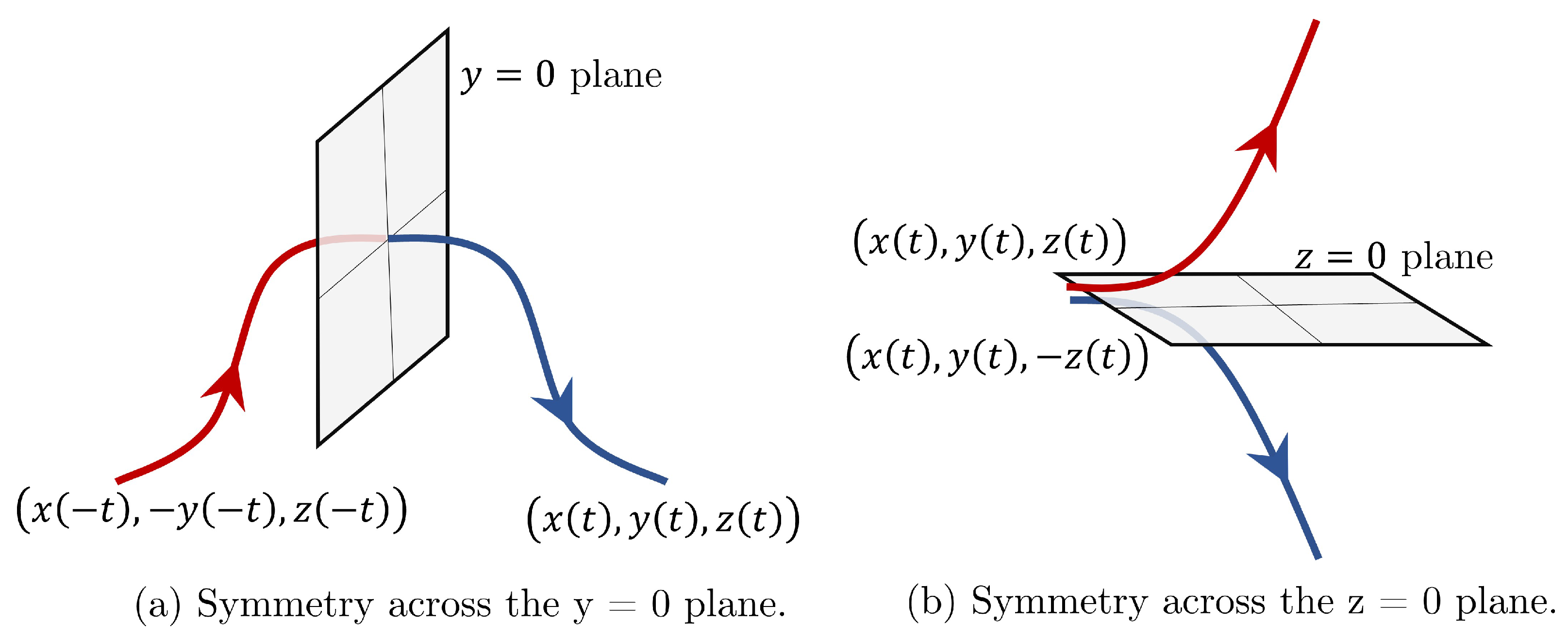
In dynamical systems theory, periodic orbits are defined as trajectories that repeat over a certain period of time. Let ${\mathit{x}}_{\mathbf{0}}={[x_0,y_0,z_0,\dot{x_0},\dot{y_0},\dot{z_0}]}^T$ and T be the initial state vector and time of flight of a spacecraft. The fundamental problem of computing a periodic orbit is finding a set of variables $\mathit{X}\equiv {[{\mathit{x}}_{\mathbf{0}},T]}^T\in {\mathbb{R}}^{7\times 1}$ that satisfies periodicity and phase conditions [14,16]. Figure 3 illustrates the periodic and phase constraints to compute a periodic orbit. Periodicity condition ensures that the propagated orbit is periodic, such that the initial state vector propagated over a time T coincides with the final state at a specific time. Periodicity condition can be conventionally expressed as

$$\mathit{\phi }({\mathit{x}}_{\mathbf{0}},0,T)-{\mathit{x}}_{\mathbf{0}}=\mathbf{0}\in {\mathbb{R}}^{6\times 1},$$

(8)

where $\mathit{\phi }({\mathit{x}}_{\mathbf{0}},0,T)$ is a terminal state vector propagated from ${\mathit{x}}_{\mathbf{0}}$ between initial and final times $t=0$ and $t=T$.

It is worth noting that the number of variables is one more than the constraints defined by the Equation (8). As a result, we add a constraint that fixes the phase of ${\mathit{x}}_{\mathbf{0}}$, allowing ${\mathit{x}}_{\mathbf{0}}$ to be found only once on the periodic orbit. The phase constraint of a periodic orbit is defined by

$$p\left({\mathit{x}}_{\mathbf{0}}\right)=\mathbf{0}\in {\mathbb{R}}^{1\times 1},$$

(9)

Combining Equations (8) and (9), the equation to find periodic solution is derived as

$$F\left(\mathit{X}\right)\equiv \left[\begin{array}{c}\mathit{\phi }({\mathit{x}}_{\mathbf{0}},0,T)-{\mathit{x}}_{\mathbf{0}}\\ p\left({\mathit{x}}_{\mathbf{0}}\right)\end{array}\right]=\mathbf{0}\in {\mathbb{R}}^{7\times 1},$$

(10)

Suitable predictor–corrector schemes can be used to trace continuous periodic family solutions that account for changes in ${\mathit{x}}_{\mathbf{0}}$ and T along the curve representing the periodic orbit family in the $({\mathit{x}}_{\mathbf{0}},T)$ plane. The predictor–corrector method proposed by [16] is considered in this work and outlined in the following subsections to provide a unique solution for Equation (10).

3.1. Predictor: Pseudo-Arclength Continuation

In this work, we use the pseudo-arclength continuation method predictor step as described in [13] to develop families of periodic orbits.

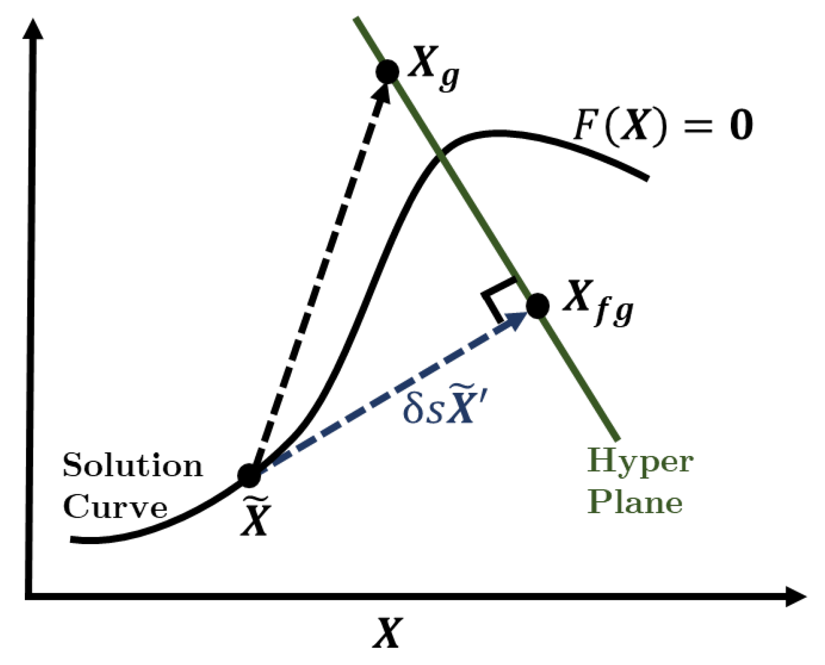
Let $\tilde{\mathit{X}}$ be a solution of $F\left(\mathit{X}\right)=0$, ${\tilde{X}}^{\prime }$ be the unit tangential vector to the curve at $\tilde{\mathit{X}}$, and $\delta s$ define prediction step size as shown in Figure 4. Then, a first guess for the next correction step ${\mathit{X}}_{\mathit{fg}}$ can be obtained along ${\tilde{X}}^{\prime }$ as

$${\mathit{X}}_{\mathit{fg}}=\tilde{\mathit{X}}\pm \delta s{\tilde{X}}^{\prime }.$$

(11)

Pseudo-arclength continuation scheme constraints to the solution guess ${\mathit{X}}_{\mathit{g}}$ can be defined by

$${({\mathit{X}}_{\mathit{g}}-\tilde{\mathit{X}})}^T{\tilde{X}}^{\prime }-\delta s=0.$$

(12)

The schematic of the pseudo-arclength continuation process is depicted in Figure 4, whereby the predictor creates a first guess at the next correction step ${\mathit{X}}_{\mathit{fg}}$ along ${\tilde{X}}^{\prime }$ with a specific step size $\delta s$. The guess ${\mathit{X}}_{\mathit{g}}$ is then iteratively corrected with a constraint Equation (12) on the orthogonal hyperplane to ${\tilde{X}}^{\prime }$ indicated as a green line in Figure 4.

The variable $\delta s$ is a small parameter (e.g., $\delta s={10}^{-4}$), whose magnitude can be adjusted throughout the continuation process to control the number of family members being computed.

3.2. Corrector: Shooting Method

The equation to be solved to correct the periodic orbits is derived by incorporating the pseudo-arclength continuation constraint Equation (12) with periodic and phase conditions of Equation (11).

$$F\left(\mathit{X}\right)\equiv \left[\begin{array}{c}\mathit{\phi }({\mathit{x}}_{\mathbf{0}},0,T)-{\mathit{x}}_{\mathbf{0}}\\ p\left({\mathit{x}}_{\mathbf{0}}\right)\\ {({\mathit{X}}_{\mathit{g}}-\tilde{\mathit{X}})}^T{\tilde{X}}^{\prime }-\delta s\end{array}\right]=\mathbf{0}.$$

(13)

Even though $({\mathit{x}}_{\mathbf{0}},T)$ from the predictor step is only a projected value, it is indeed unlikely that each of Equation (13)’s constraints are satisfied. The predicted solution is, however, close to the true solution; Newton’s method can be used to numerically iterate the predicted solution until Equation (13) converges to zero or close to a tolerance margin. Now, defining $\mathsf{\Delta }\mathit{X}$ as the correction vector of ${\mathit{X}}_{\mathit{g}}$, the objective function at the next guess can be given by first-order Taylor’s expansion:

$$F({\mathit{X}}_{\mathit{g}}+\mathsf{\Delta }\mathit{X})=F\left({\mathit{X}}_{\mathit{g}}\right)+{\displaystyle \frac{\partial F\left({\mathit{X}}_{\mathit{g}}\right)}{\partial X_g}}\mathsf{\Delta }\mathit{X}+HigherOrderTerms(H.O.T.)$$

(14)

where ${\displaystyle \frac{\partial F}{\partial X_g}}$ is the Jacobian and expressed as

$${\displaystyle \frac{\partial F\left({\mathit{X}}_{\mathit{g}}\right)}{\partial X_g}}=\left[\begin{array}{cc}{\displaystyle \frac{\partial \mathit{\phi }}{\partial {\mathit{x}}_{\mathbf{0}}}}& \dot{\mathit{\phi }}({\mathit{x}}_{\mathbf{0}},0,T)\\ {\displaystyle \frac{\partial p\left({\mathit{x}}_{\mathbf{0}}\right)}{\partial {\mathit{x}}_{\mathbf{0}}}}& 0\\ {{\tilde{X}}^{\prime }}_{{\mathit{x}}_{\mathbf{0}}}^T& {{\tilde{X}}^{\prime }}_{\mathit{T}}^T\end{array}\right]$$

(15)

where ${\displaystyle \frac{\partial \phi }{\partial {\mathit{x}}_{\mathbf{0}}}}$ corresponds to the state transition matrix (STM) from ${\mathit{x}}_{\mathbf{0}}$ to $\mathit{\phi }({\mathit{x}}_{\mathbf{0}},0,T)$. STM after one orbital period is also known as monodromy matrix, M, which helps analyze the stability of the computed periodic orbits in the next subsection. ${{\tilde{X}}^{\prime }}_{\mathit{x}\mathbf{0}}^T$ and ${{\tilde{X}}^{\prime }}_{\mathit{T}}^T$ are components of ${\tilde{X}}^{\prime }$ updating ${\mathit{x}}_{\mathbf{0}}$ and T, respectively.

On eliminating the higher order terms from Equation (14), the periodic solution $F\left(\mathit{X}\right)$ is converged by iteratively updating the $\mathsf{\Delta }\mathit{X}$ vector.

$$\mathsf{\Delta }\mathit{X}=-{\left(\begin{array}{c}{\displaystyle \frac{\partial F\left({\mathit{X}}_{\mathit{g}}\right)}{\partial X_g}}\end{array}\right)}^{-1}F\left({\mathit{X}}_{\mathit{g}}\right)$$

(16)

Upon convergence, the algorithm solves the boundary value problem, which allows the predictor–corrector scheme to be reinitialized and continue along the branch of the periodic orbit family.

3.3. Bifurcated Retrograde Families

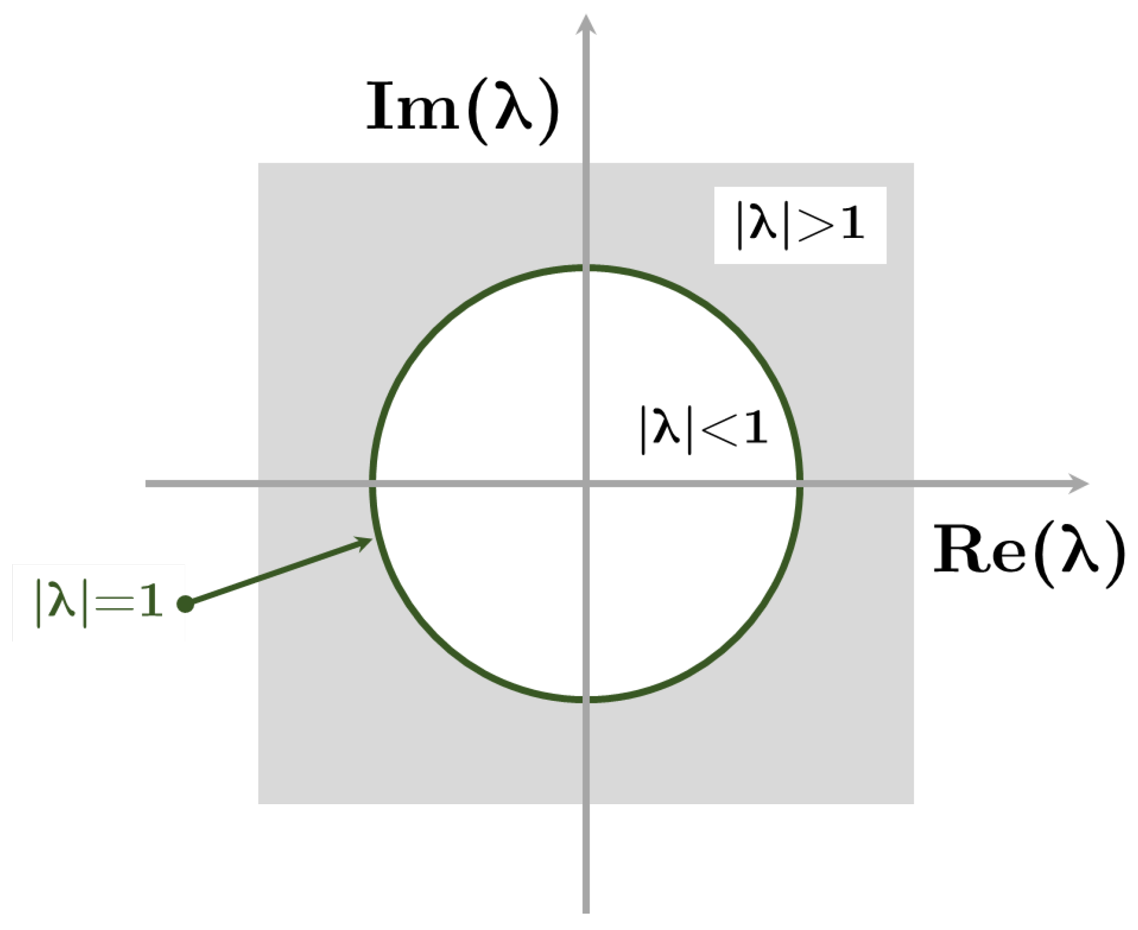
The monodromy matrix, M, defined as the state transition matrix propagated for exactly one period of the orbit, is commonly used to determine orbital stability. Let $\delta {\mathit{x}}_{\mathbf{0}}$ be a small perturbation about the initial state of the computed periodic orbit. State transition matrix maps this initial deviation forward in time after ’n’ orbital periods.

$$\begin{array}{cc}\hfill \delta {\mathit{x}}_{\mathbf{n}}& =\mathsf{\Phi }(T_n,t_0)\delta {\mathit{x}}_{\mathbf{0}}\hfill \\ & =\mathsf{\Phi }(T_n,T_{n-1})\dots \mathsf{\Phi }(T,t_0)\delta {\mathit{x}}_{\mathbf{0}}=M^n\delta {\mathit{x}}_{\mathbf{0}}\hfill \end{array}$$

(17)

Following the nature of Hamiltonian dynamical systems, for each eigenvalue $\lambda \in \mathbb{R}$ of M, $1/\lambda$ is also an eigenvalue, and occurs in reciprocal pairs [42,43]. Also, if $\lambda \in \mathbb{C}$, then $\overline{\lambda }$ and $1/\overline{\lambda }$ are eigenvalues of M. Periodic orbits are stable only when all of the eigenvalues (${\lambda }_i,\forall i=1,2,..,n$) of M have a magnitude less than unity, i.e., $|{\lambda }_i|\le 1,\forall i=1,2,..,n$.

Figure 5 illustrates the stability bounds for eigenvalues of the monodromy matrix in the complex plane to the unit circle. Non-trivial and complex eigenvalues placed on the unit circle ($\left|\lambda \right|=1$) indicate the existence of oscillatory modes. A pair of reciprocal eigenvalues that are placed off the unit circle, on the other hand, indicates the presence of unstable ($\left|\lambda \right|>1$) and stable ($\left|\lambda \right|<1$) modes governing the motion in the vicinity of the periodic orbit. Bifurcation occurs when a pair of non-trivial eigenvalues reach any critical value, which will be discussed in the following subsection.

Let ${\mathit{\phi }}_T\left({\mathit{x}}_{\mathbf{0}}\right)={\mathit{x}}_{\mathbf{0}}$ be the periodic solution of Equations of motion, then

$${\mathit{\phi }}_T({\mathit{x}}_{\mathbf{0}}+\delta {\mathit{x}}_{\mathbf{0}})\simeq {\mathit{\phi }}_T\left({\mathit{x}}_{\mathbf{0}}\right)+M\delta {\mathit{x}}_{\mathbf{0}}+H.O.T.={\mathit{x}}_{\mathbf{0}}+\delta {\mathit{x}}_{\mathbf{0}}.$$

(18)

Neglecting H.O.T. yields $(M-I_n)\delta {\mathit{x}}_{\mathbf{0}}=0$, where $I_n$ is an identity matrix, resulting with an eigenvalue $\lambda =1$. If this is true, a second eigenvalue must be equal to unity as well. Furthermore, the characteristic polynomial of a 6-by-6 monodromy matrix can be further simplified as

$$\begin{array}{cc}\hfill det(M-\lambda I_n)& ={(\lambda -1)}^2(\lambda -{\lambda }_1)(\lambda -1/{\lambda }_1)(\lambda -{\lambda }_2)(\lambda -1/{\lambda }_2),\hfill \\ \hfill & ={(\lambda -1)}^2({\lambda }^2+b_1\lambda +1)({\lambda }^2+b_2\lambda +1),\hfill \end{array}$$

(19)

where ${\lambda }_1$, $1/{\lambda }_1$, ${\lambda }_2$, $1/{\lambda }_2$ are other non-trivial eigenvalues of M, and $b_1=-({\lambda }_1+1/{\lambda }_1)$ and $b_2=-({\lambda }_2+1/{\lambda }_2)$ must be real with $max\left(\right|Re\left(b_1\right)|,|Re\left(b_2\right)\left|\right)<2$ for a periodic orbit to be stable.

Values $b_1$ and $b_2$ are referred to as stability indices and will be evaluated throughout this thesis to assess the stability of the periodic orbits [42,44]. Following [45], $b_1$ and $b_2$ are calculated as

$$b_1,b_2={\displaystyle \frac{\alpha \pm \sqrt{{\alpha }^2-4\beta +8}}{2}},$$

(20)

where $\alpha =2-trace\left(M\right)$ and $\beta ={\displaystyle \frac{{\alpha }^2-trace\left(M^2\right)}{2}}+1$,

$$1/{\lambda }_j,{\lambda }_j={\displaystyle \frac{-b_j\pm \sqrt{b_j^2-4}}{2}},\forall j=1,2,$$

(21)

Equation (21) provides an efficient relation for computing the eigenvalues of the monodromy matrix of any periodic orbit of a six-dimensional autonomous Hamiltonian system.

Naturally, once the eigenvalues of M are known, the resulting eigenvectors can be used to compute the invariant manifolds associated with the periodic orbit. The invariant manifolds of a periodic orbit are computed by perturbing the states along the direction of periodic orbit’s local eigenvectors.

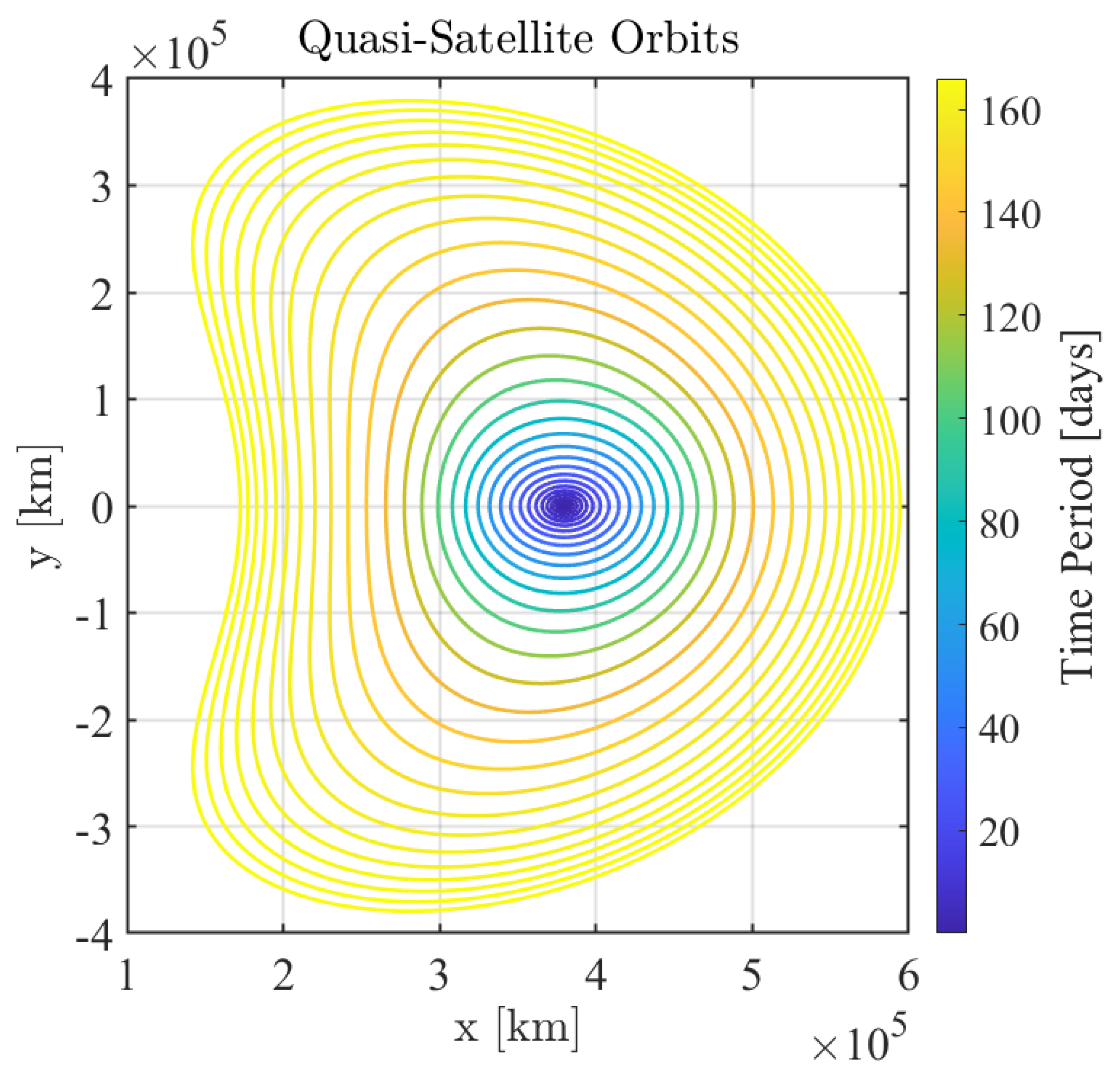
QSOs are retrograde periodic orbits existing around the smaller primary. They are also known as DROs and family-f orbits. QSOs are generally considered one of the three kinds of co-orbital configurations in CRTBP with 1:1 resonance. In this research, we have utilized pseudo-arclength continuation and shooting methods for calculating planar QSO families, as shown in the Figure 6.

The periodic orbits of the retrograde family branch obtained through the pseudo-arclength continuation method are shown in Figure 7 with the stability indices of each family branch computed from Equation (22).

$$b_j\equiv {\lambda }_j+{\displaystyle \frac{1}{{\lambda }_j}},j=1,2.$$

(22)

As shown by the linear analysis indicated by the stability indices of the periodic orbit monodromy matrix eigenvalues, these relative orbits are linearly stable (i.e., when stability index $b_j<2$). In a Hamiltonian system, the monodromy matrix of a periodic orbit, M ($d\Phi (x,T)/dx$) is the state transition matrix of a periodic orbit after one time period and has three pairs of eigenvalues with one trivial pair $D=1$. We bifurcate the planar family using their stability indices defined as in Equation (22) [43,44], where ${\lambda }_j$ and 1/${\lambda }_j$ are jth reciprocal eigenvalues pairs of monodromy matrix M.

$$b_{Res}=2cos2\pi {\displaystyle \frac{d}{n}},d,n\in N$$

(23)

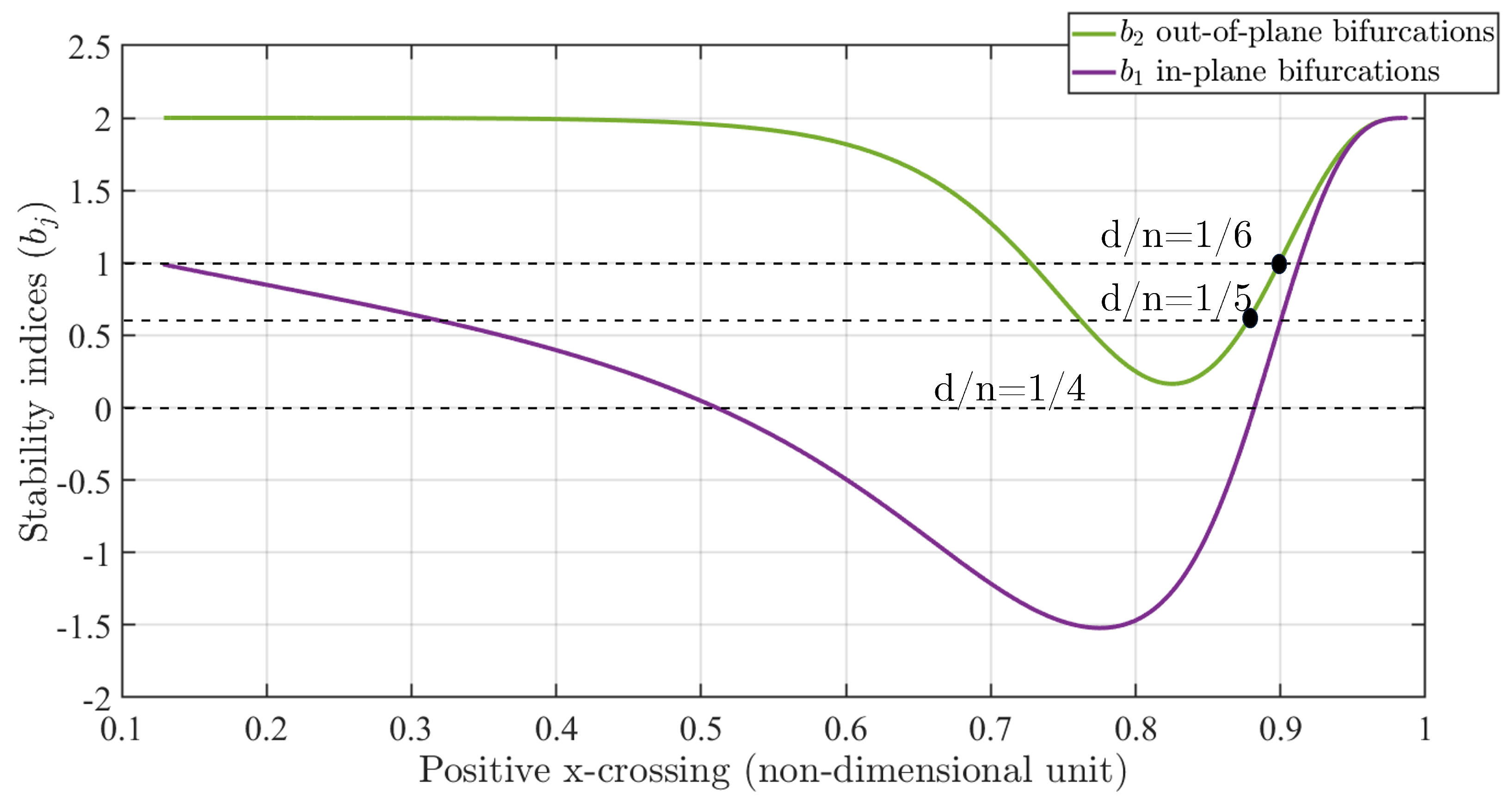
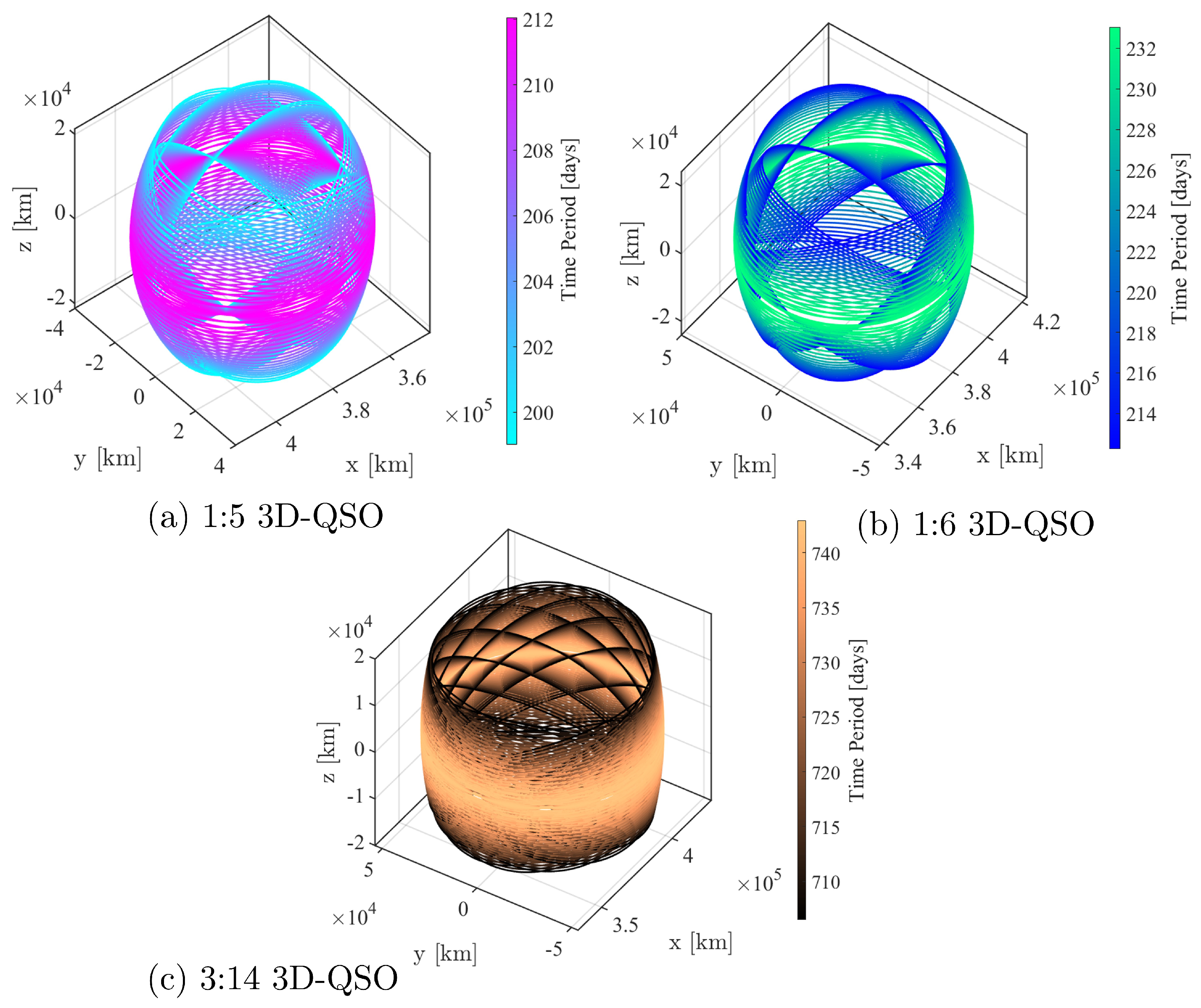
Important characteristics of stability indices are when they reach any resonant value $(d/n)$, and the state corresponds to a bifurcation point indicated using Equation (23) [11,46,47]. In the literature, periodic orbits bifurcating via in-plane perturbations are $swingQSOs$ or $MP$-$QSOs$ [48,49,50], and the members bifurcating from out-of-plane perturbations are $3D$-$QSOs$. In this work, we consider the out-of-plane bifurcated families of both retrograde and prograde orbits. An example of bifurcated out-of-plane retrograde orbit of $(d/n)$ = 1/5, $(d/n)$ = 1/6, and $(d/n)$ = 3/14 with $b_{Res}$ of 0.618, 1 and 0.445 are shown within Figure 8. Figure 9 illustrates the 3D or spatial members of QSOs or DROs branching out from the planar families of DRO in the Earth–Moon CRTBP system. The colors blue and red represent the stable and unstable members of the computed families. A more detailed description of the computation and classification of these families is provided in [51,52], where bifurcation conditions and stability criteria are analyzed comprehensively.

4. Trajectory Optimization

In highly nonlinear dynamics, such as those of the CRTBP, it is challenging to identify low-thrust optimal solutions. Optimization problems cannot be solved without the capacity to generate accurate initial guesses [53,54]. In the design of transfer trajectories between retrograde orbits, the orbit-chaining method is one of the approaches to make reasonable initial guesses. More specifically, this method utilizes natural dynamical structures such as periodic orbits and their invariant manifolds in order to connect trajectories from one orbit to another. An illustration of this method can be found in Figure 10. The choice of intermediate trajectories and the order in which they are created affect the initial estimate produced by the orbit-chaining method. The CRTBP employs the Jacobi constant as an efficient index in order to choose appropriate sequences of intermediate trajectories.

4.1. Initial Guesses Based on Orbit Chaining

In this paper, we consider the case of planar-to-spatial QSO transfer trajectories constructed along the 1:5 3D-QSO family (Figure 8a) and the planar QSO by minimizing fuel consumption. As shown in Figure 8a, this paper focuses on 50 1:5 3D-QSO orbits bifurcated from the family of planar orbits shown in Figure 8a and Figure 9 with their time period. We assume that the initial points of transfer trajectories between these intermediate orbits lie in their apolunes.

4.2. Optimal Control Problem

Based on Equation (1), the equations of motion of $P_3$ with control inputs are given by

$$\left\{\begin{array}{cc}\hfill \ddot{x}-2\dot{y}& ={\displaystyle \frac{\partial U}{\partial x}}+u_x\hfill \\ \hfill \ddot{y}+2\dot{x}& ={\displaystyle \frac{\partial U}{\partial y}}+u_y.\hfill \\ \hfill \ddot{z}& ={\displaystyle \frac{\partial U}{\partial z}}+u_z\hfill \end{array}\right.$$

(24)

Equation (24) can be simply expressed as

$$\begin{array}{cc}\hfill \dot{\mathit{x}}& =f\left(\mathit{x}\right)+B\mathit{u},\hfill \end{array}$$

(25)

$$\begin{array}{cc}\hfill B& =\left[\begin{array}{c}{O}_{3\times 3}\\ I_{3\times 3}\end{array}\right],\hfill \end{array}$$

(26)

where the state vector $\mathit{x}={\left[x,y,z,\dot{x},\dot{y},\dot{z}\right]}^{\mathrm{T}}$ and the control input vector $\mathit{u}={\left[u_x,u_y,u_z\right]}^{\mathrm{T}}$. The control input vector $\mathit{u}$ is constrained by the norm of the control input u such that

$$u_x^2+u_y^2+u_z^2=u^2.$$

(27)

Because the change in the mass of $P_3$ is neglected, maximum thrust acts as maximum acceleration. For a low-thrust control problem, a constraint for the maximum acceleration $u_{\max }$ is defined as follows:

$$u\le u_{\max }.$$

(28)

The optimal control problem is a two-point boundary value problem; the boundary values $x_0$ and $x_{\mathrm{f}}$ at the initial and final time $t_0$, $t_{\mathrm{f}}$, respectively, are fixed through the optimization process such that

$$\begin{array}{cccc}\hfill \mathit{x}\left(t_0\right)& ={\mathit{x}}_0,\hfill & \hfill \mathit{x}\left(t_{\mathrm{f}}\right)& ={\mathit{x}}_{\mathrm{f}}.\hfill \end{array}$$

(29)

The objective function of this problem is given by

$$J={\int }_{t_0}^{t_{\mathrm{f}}}u\left(t\right)dt.$$

(30)

The integral of u equals the amount of the velocity change $\mathsf{\Delta }V$, so this objective function J is regarded as the fuel consumption. The optimization problem (Equations (25)–(30)) is summarized as follows:

$$\begin{array}{cccc}\hfill & \mathrm{minimize}\hfill & \hfill & J={\int }_{t_0}^{t_{\mathrm{f}}}u\left(t\right)dt,\hfill \\ \hfill & \mathrm{subject}\mathrm{to}\hfill & \hfill & \dot{\mathit{x}}=f\left(\mathit{x}\right)+B\mathit{u},\hfill \\ \hfill & \hfill & & \mathit{x}\left(t_0\right)={\mathit{x}}_0,\mathit{x}\left(t_{\mathrm{f}}\right)={\mathit{x}}_{\mathrm{f}},\hfill \\ \hfill & \hfill & & u_x^2+u_y^2+u_z^2=u^2,u\le u_{\max }.\hfill \end{array}$$

(31)

This low-thrust optimization problem aims to optimize the time history of the control input vector $\mathit{u}$ to minimize the fuel consumption J under the constraints. Note that $t_0$ and $t_{\mathrm{f}}$ remain constant through the optimization.

4.3. Successive Convex Optimization

In this subsection, the successive convex optimization method is applied to the optimization problem of Equation (31) [33,35]. The constraints of Equations (25) and (27) are non-convex, so it is necessary to transform them into convex constraints. First, Equation (27) is converted to a convex constraint by including the interior of this constraint and expressed as

$$u_x^2+u_y^2+u_z^2\le u^2.$$

(32)

This relaxation belongs to lossless convexification, because it is proved that this modification does not change the optimal solutions to be obtained [33]. Next, Equation (25) is linearized in the vicinity of a reference trajectory ${\mathit{x}}^{*}$ as follows:

$$\begin{array}{cc}\hfill \dot{\mathit{x}}& =f\left({\mathit{x}}^{*}\right)+A\left(t\right)\left(\mathit{x}-{\mathit{x}}^{*}\right)+B\mathit{u},\hfill \end{array}$$

(33)

$$\begin{array}{cc}\hfill A\left(t\right)& =\left[\begin{array}{cccccc}0& 0& 0& 1& 0& 0\\ 0& 0& 0& 0& 1& 0\\ 0& 0& 0& 0& 0& 1\\ {\left.{\displaystyle \frac{{\partial }^{2}U}{{\partial }^{2}x}}\right|}_{{\mathit{x}}^{*}}& {\left.{\displaystyle \frac{{\partial }^{2}U}{\partial x\partial y}}\right|}_{{\mathit{x}}^{*}}& {\left.{\displaystyle \frac{{\partial }^{2}U}{\partial x\partial z}}\right|}_{{\mathit{x}}^{*}}& 0& 2& 0\\ {\left.{\displaystyle \frac{{\partial }^{2}U}{\partial y\partial x}}\right|}_{{\mathit{x}}^{*}}& {\left.{\displaystyle \frac{{\partial }^{2}U}{{\partial }^{2}y}}\right|}_{{\mathit{x}}^{*}}& {\left.{\displaystyle \frac{{\partial }^{2}U}{\partial y\partial z}}\right|}_{{\mathit{x}}^{*}}& -2& 0& 0\\ {\left.{\displaystyle \frac{{\partial }^{2}U}{\partial z\partial x}}\right|}_{{\mathit{x}}^{*}}& {\left.{\displaystyle \frac{{\partial }^{2}U}{\partial z\partial y}}\right|}_{{\mathit{x}}^{*}}& {\left.{\displaystyle \frac{{\partial }^{2}U}{{\partial }^{2}z}}\right|}_{{\mathit{x}}^{*}}& 0& 0& 0\end{array}\right].\hfill \end{array}$$

(34)

Equation (33) is rewritten as

$$\dot{\mathit{x}}=A\left(t\right)\mathit{x}+B\mathit{u}+\left\{f\left({\mathit{x}}^{*}\right)-A\left(t\right){\mathit{x}}^{*}\right\}.$$

(35)

The third term $f\left({\mathit{x}}^{*}\right)-A\left(t\right){\mathit{x}}^{*}$ is the time-varying term determined only by ${\mathit{x}}^{*}$. In the calculation, the $(i-1)$-th optimal trajectory is regarded as the reference trajectory for the i-th iteration. Hence, Equation (33) becomes

$${\dot{\mathit{x}}}^{\left(i\right)}=f\left({\mathit{x}}^{(i-1)}\right)+A\left(t\right)\left({\mathit{x}}^{\left(i\right)}-{\mathit{x}}^{(i-1)}\right)+B{\mathit{u}}^{\left(i\right)}.$$

(36)

When the deviation ${\mathit{x}}^{\left(i\right)}-{\mathit{x}}^{(i-1)}$ becomes zero, the i-th optimal trajectory ${\mathit{x}}^{\left(i\right)}$ satisfies nonlinear dynamics described as

$${\dot{\mathit{x}}}^{\left(i\right)}=f\left({\mathit{x}}^{(i-1)}\right)+B{\mathit{u}}^{\left(i\right)}.$$

(37)

For a guarantee of the convergence of the deviation, a new constraint is introduced as follows:

$$max\left(\left|\mathit{x}-{\mathit{x}}^{(i-1)}\right|\right)\le \gamma max\left(\left|{\mathit{x}}^{(i-1)}-{\mathit{x}}^{(i-2)}\right|\right),$$

(38)

where $\gamma$ is a constant for determining the convergence rate. However, in the first iteration, the trust region $\delta$ is introduced such that

$$max\left(\left|\mathit{x}-{\mathit{x}}^{(i-1)}\right|\right)\le \delta ,$$

(39)

instead of Equation (38). Since the deviation $\mathit{x}-{\mathit{x}}^{(i-1)}$ cannot be reduced to completely zero in the numerical calculation, the iteration is terminated when

$$max\left(\left|\mathit{x}-{\mathit{x}}^{(i-1)}\right|\right)\le \epsilon ,$$

(40)

where $\epsilon$ is the termination condition. In this study, we set $\epsilon$ = 1 ×${10}^{-4}$, expressed in non-dimensional CRTBP units, based on trade-offs observed during preliminary testing; this threshold provided reliable convergence without excessive computational burden.

For the numerical calculation of the optimization problem, this problem is discretized into a finite-dimensional problem with the sampling time $h_k$. The subscript k means a discrete node index. It is assumed that the sampling time $h_k$ is different for each discrete node and is discretized by a zero-order hold. The discretized equation of motion is expressed as

$${\mathit{x}}_{k+1}=A_k{\mathit{x}}_k+B_k{\mathit{u}}_k+F_k,$$

(41)

where

$$\begin{array}{cc}\hfill A_k& =\varphi (t_k+h_k,t_k),\hfill \end{array}$$

(42)

$$\begin{array}{cc}\hfill B_k& ={\int }_{t_k}^{t_k+h_k}\varphi (t_k+h_k,\tau )Bd\tau =\eta (t_k+h_k,t_k),\hfill \\ \hfill F_k& ={\int }_{t_k}^{t_k+h_k}\varphi (t_k+h_k,\tau )\left\{f\left({\mathit{x}}^{*}\right)-A\left(\tau \right){\mathit{x}}^{*}\right\}d\tau \hfill \end{array}$$

(43)

$$\begin{array}{cc}\hfill & =\zeta (t_k+h_k,t_k),\hfill \end{array}$$

(44)

$$\begin{array}{cc}\hfill {\displaystyle \frac{d}{dt}}\varphi (t,t_k)& =A\left(t\right)\varphi (t,t_k),\hfill \end{array}$$

(45)

$$\begin{array}{cc}\hfill {\displaystyle \frac{d}{dt}}\eta (t,t_k)& =A\left(t\right)\eta (t,t_k)+B,\hfill \end{array}$$

(46)

$$\begin{array}{cc}\hfill {\displaystyle \frac{d}{dt}}\zeta (t,t_k)& =A\left(t\right)\zeta (t,t_k)+f\left({\mathit{x}}^{*}\right)-A\left(t\right){\mathit{x}}^{*},\hfill \end{array}$$

(47)

$$\begin{array}{cc}\hfill \varphi (t_k,t_k)& =I_{6\times 6},\eta (t_k,t_k)=O_{6\times 3},\zeta (t_k,t_k)=O_{6\times 1},\hfill \end{array}$$

(48)

where $t_k\le t\le t_k+h_k$ and $k=1,2,3,\dots$. The objective function of Equation (30) is also discretized as follows:

$$J=\sum _k{u}_k{h}_k.$$

(49)

In the calculation, the discrete node points are determined with equal time intervals along each halo orbit in the initial guess, and each of the halo orbits has N discrete node points.

Consequently, when the whole trajectory of the initial guess is discretized into M points, the optimization problem to solve in this paper is summarized as follows:

$$\begin{array}{cccc}\hfill & \mathrm{minimize}\hfill & \hfill & J=\sum _{k=1}^{M-1}{u}_k{h}_k,\hfill \\ \hfill & \mathrm{subject}\mathrm{to}\hfill & \hfill & {\mathit{x}}_{k+1}=A_k{\mathit{x}}_k+B_k{\mathit{u}}_k+F_k,\hfill \\ \hfill & \hfill & & {\mathit{x}}_1={\mathit{x}}_{\mathrm{ini}},{\mathit{x}}_M={\mathit{x}}_{\mathrm{fin}},\hfill \\ \hfill & \hfill & & u_{k,x}^2+u_{k,y}^2+u_{k,z}^2\le u_k^2,u_k\le u_{\max },\hfill \\ \hfill & \hfill & & max\left(\left|\mathit{x}-{\mathit{x}}^{(i-1)}\right|\right)\hfill \\ \hfill & \hfill & & \le \gamma max\left(\left|{\mathit{x}}^{(i-1)}-{\mathit{x}}^{(i-2)}\right|\right).\hfill \end{array}$$

(50)

This convex optimization problem is classified as second-order cone programming. The software CVX for MATLAB is applied to solve this problem [55]. The key steps of the successive convexification procedure are summarized in Algorithm 1, which outlines the iterative process used to linearize, solve, and update the trajectory at each step until convergence.

Algorithm 1: Successive convexification method for low-thrust transfer.

5. Intermediate Orbit Design for Transfers

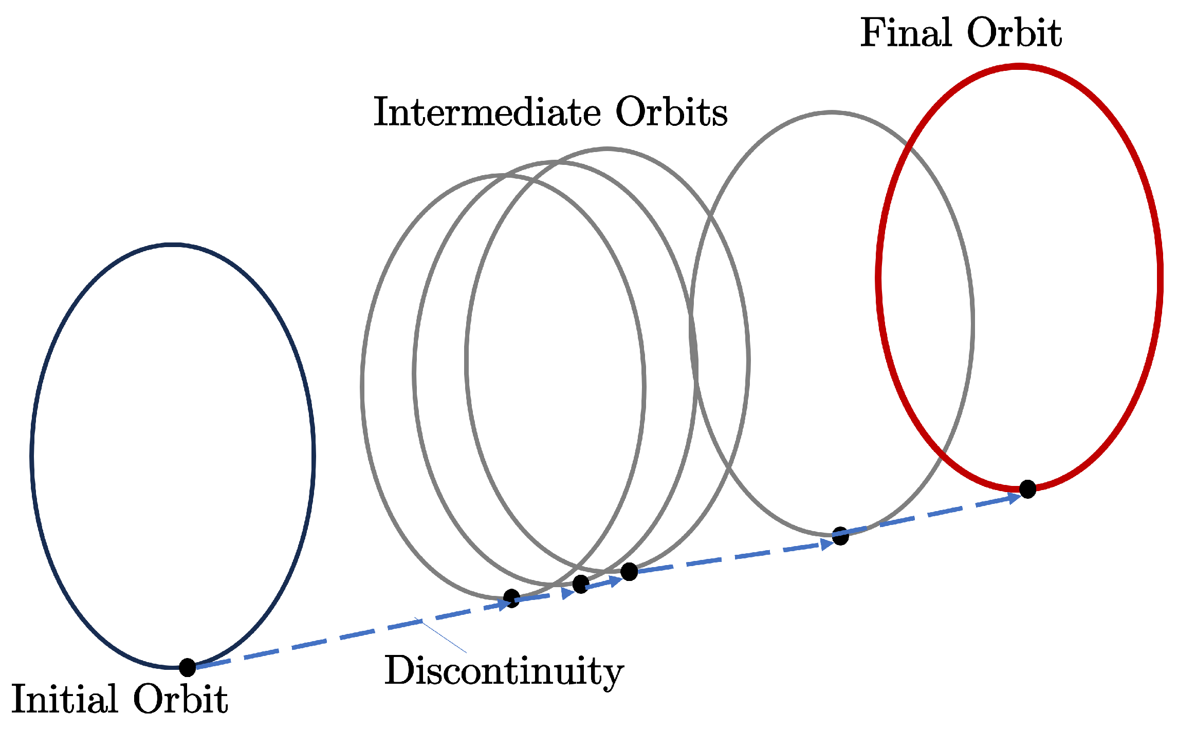
This part introduces the intermediate orbit design methodology for systematically investigating minimum total $\mathsf{\Delta }$ V planar QSO to 3D-QSO low-thrust transfers. Instead of relying solely on heuristic orbit chains, we construct initial guess sequences using a beam search algorithm adapted to the QSO topology. Unlike our previous application to halo orbits, QSOs exhibit richer bifurcation structures, making naïve sequencing less effective. We generate candidate sequences by evaluating subsets of planar and spatial QSOs, ranking them based on the estimated $\mathsf{\Delta }$V of their connecting segments using short propagation arcs. Only the top candidates $\alpha$ (beam width) are expanded at each depth, effectively pruning the search space while preserving diverse solution paths.

Each guess is passed to the convex solver as a piecewise arc concatenation, and solutions are retained if they converge within a bounded number of iterations. This framework allows us to explore a broader set of orbit families while keeping computational cost tractable. To build the best possible transfer by utilizing natural dynamics, prospective intermediate orbits are selected from the chosen 1:5 3D-QSO family. Based on the beam search algorithm, the suggested algorithm makes initial guesses for the transfers between a given initial and end orbit and then inserts a candidate orbit into the resulting series of intermediate family members of 1:5 3D-QSOs. The suggested approach has proven to efficiently search for the minimal total $\mathsf{\Delta }$V transfer solutions by exploiting the generated initial guesses in the case of halo–halo transfer. The success of the proposed technique is heavily dependent on the evaluation index at each tree depth and this evaluation index is the total $\mathsf{\Delta }$V, the difference in $\mathsf{\Delta }$V between the first and final orbits.

5.1. Transfer Methodology: Tree-Search Method

The breadth-first and depth-first approaches are widely recognized as the most frequently used tree-search algorithms. The breadth-first (BFS) approach systematically traverses all nodes inside a given tree by exploring each level before proceeding to the next. In contrast, the depth-first (DFS) approach explores each branch as extensively as possible before backtracking. If the search tree involves a loop, the DFS algorithm may become stuck indefinitely, as it may ascend a branch that continually hops between two nodes. Depth-limited search (DLS) is presented to remedy the situation. With this approach, the tree cannot expand beyond a fixed height that is determined beforehand. 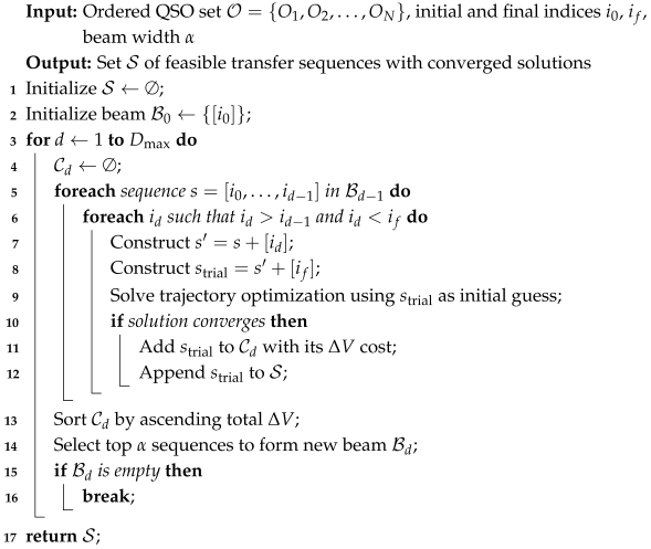If the branch is too long, it will eventually be void and be replaced by a new one [55]. The detailed steps of the beam search process are formalized in Algorithm 2, which systematically expands promising intermediate sequences between the initial and final QSOs. The method maintains a beam of the top sequences at each level based on total, ensuring a balance between computational efficiency and solution diversity.

Table 1. Notations used in the beam search algorithm for QSO transfer design.

Symbol	Description
$\mathcal{O}=\{O_1,O_2,\dots ,O_N\}$	Ordered set of candidate quasi-satellite orbits
$i_0$	Index of the initial QSO
$i_f$	Index of the final QSO
$\alpha$	Beam width (number of branches retained at each depth)
$D_{max}$	Maximum tree depth (number of intermediate QSOs allowed)
s	A candidate sequence of QSO indices
$s^{\prime }$	Extended sequence obtained by appending one orbit to s
$s_{\mathrm{trial}}$	Trial sequence including final orbit $i_f$
${\mathcal{C}}_d$	Set of converged candidate sequences at depth d
${\mathcal{B}}_d$	Beam at depth d: top $\alpha$ from ${\mathcal{C}}_d$
$\mathcal{S}$	Final set of feasible transfer sequences
$\mathsf{\Delta }V$	Total delta-V cost for a given sequence

summarizes the notations used throughout the algorithm.

Algorithm 2: Beam search for intermediate QSO selection.

5.2. Beam Search of Intermediate Transfer Orbits

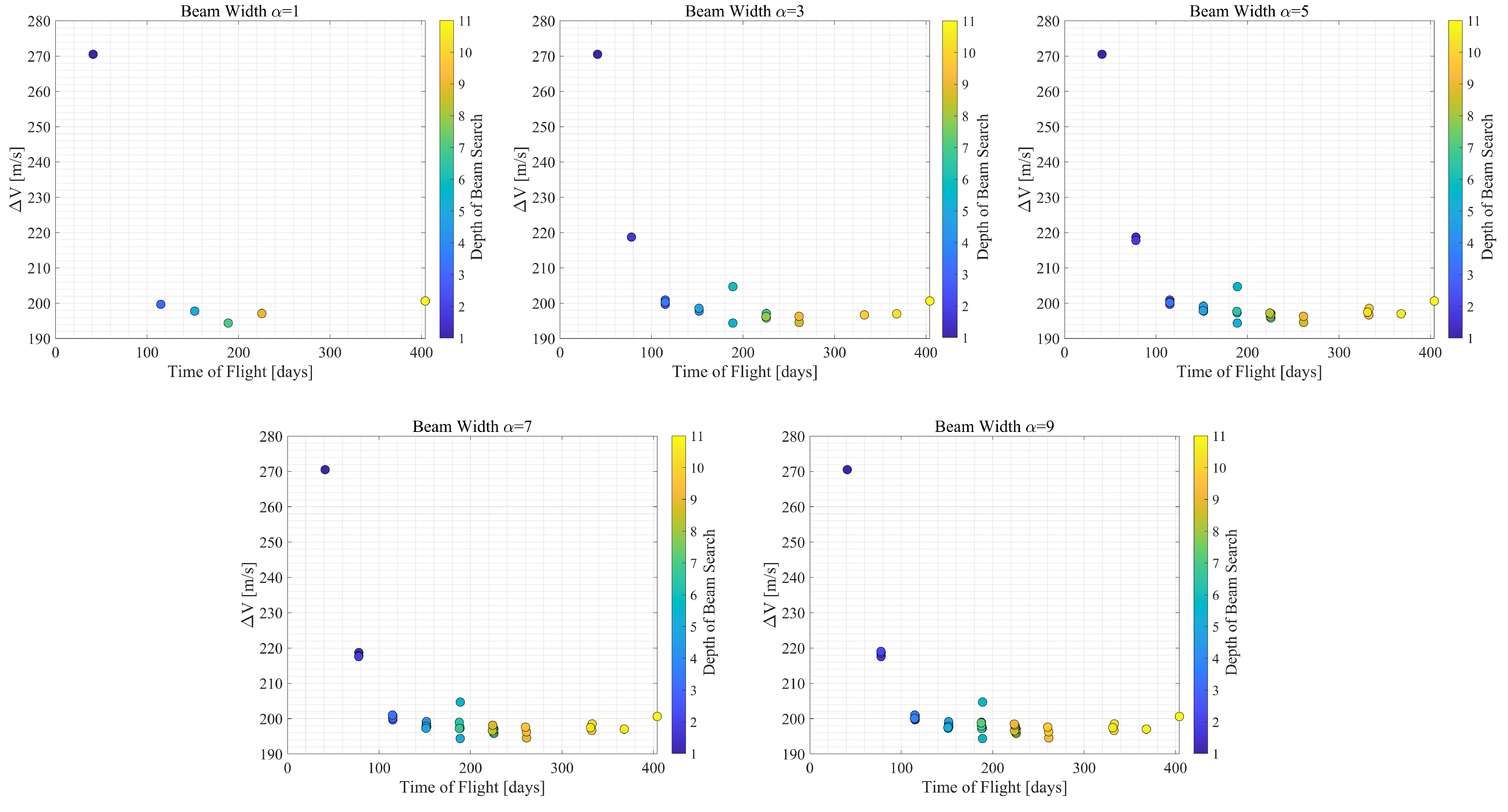
The beam search algorithm is a heuristic approach that shares similarities with the breadth-first search algorithm in its application to optimization problems [56]. The approach has been implemented in artificial intelligence, complex scheduling, and space engineering [57]. The distinction between the breadth-first method and the approach described here resides in the selective branching from only the most promising nodes, referred to as beam nodes, at each tree level. The parameter $\alpha$, known as the beam width, determines the number of nodes to be considered for branching. The computational time required by the beam search technique is comparatively brief due to its ability to significantly reduce the search space by restricting the search to a subset of potential solutions determined by the beam width parameter $\alpha$.

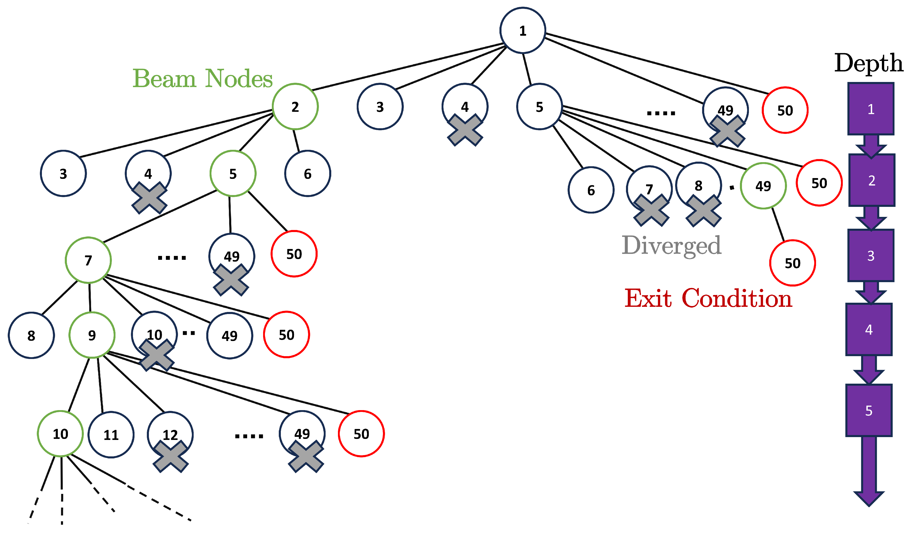
The first step would be the computation and evaluation of the initial guess. To begin the process, a successive convex optimization with initial guesses (i.e.,$[1,j](j=2,3,...,50)$), in this case, planar QSO at the point of bifurcation and 48 members of 3D-QSO families to connect with the desired final orbit of the 1:5 3D-QSO family and evaluate each node branching out from the planar QSO and estimate the $\mathsf{\Delta }$V. The evaluation index is $\mathsf{\Delta }$V; that is, the $\alpha$ beam nodes are selected from the nodes in ascending order, corresponding to each $\mathsf{\Delta }$V. The nodes that do not converge are disregarded, and the exit condition is evaluated (i.e., node 50, the final 3D-QSO). The optimization results and the sequence of the intermediate orbits related to such nodes are stored as local optimal solutions.

The next step would be branching out from beam nodes. To branch out from each beam node, new nodes are generated so that their node number is larger than the node number of the beam node. For example, when $\alpha =3$, to branch out from the beam node ‘No.5’, the sequence of $[1,5,j](j=6,7,...,50)$ is evaluated. After dismissing the nodes related to diverged solutions and judging the exit condition, the rest of the nodes are considered by the total $\mathsf{\Delta }$V between the planar QSO ‘No.1’ and final 3D-QSO (1:5 family) ‘No. j’ to determine one beam node (the node with the lowest total $\mathsf{\Delta }$V) for this tree depth. If no nodes are left after the exit condition evaluation, the calculation along with this phyletic line stops, and the number of beam nodes is reduced in the next tree depth.

The algorithm’s final phase will expand the tree created by the previous step until the number of beam nodes reaches zero. When all calculations have been finished, the optimization results of the nodes that satisfy the exit criterion at each tree depth are compiled, and the initial guess with the lowest total V is found. As a result, the proposed technique can systematically search for a favorable sequence of intermediary 1:5 3D-QSOs along the family’s Jacobi constant curve. The results of this simulation for the case of 1:5 3D-QSO are discussed in the following section. It can be noted that the same approach can be applied to other periodic orbit families in the CRTBP.

6. Results and Discussions

6.1. Transfers Between Planar QSO and 1:5 3D-QSO

This section applies the beam search algorithm discussed in the previous section to design low-thrust transfer trajectories between a planar QSO and a 1:5 3D-QSO using intermediate family members of the 3D-QSO family. The parameters for successive convex optimization discussed in Section 4.3 are selected based on [12,35] and shown in

Table 2. Parameters for the successive convex optimization.

Parameter	Symbol	Value
Discrete node number	N [per period]	500
Maximum acceleration	$u_{max}$ [m/s2]	$1\times {10}^{-4}$
Terminate condition	$ϵ$ [-]	$1\times {10}^{-4}$
Convergence rate	$\gamma$ [-]	0.8
Trust region	$\delta$ [-]	$1\times {10}^{-4}$

. In this work, we will discuss the case of results with the beam width $\alpha$ = 1, 3, 5, 7, 9, which are summarized in Figure 11. The obtained optimal trajectory and control history of the $\mathsf{\Delta }$$V_{min}$ solution are shown in Figure 12 and Figure 13. The blue and red lines in Figure 12 denote coasting and thrusting arcs, respectively. Figure 13 demonstrates that the norm of control inputs is smaller than the maximum acceleration $u_{max}$ in the thrusting arcs and in the coasting arcs. In Figure 11, we find that the beam search algorithm finds more local optimal solutions as the beam width increases. The obtained local optimal solutions have various total $\mathsf{\Delta }$V and ToF.

Figure 11 represents the total $\mathsf{\Delta }$V and ToF of the local optimal solutions when the beam width $\alpha$ = 1, 3, 5, 7, 9. The depth of beam search in the color bar is equivalent to the tree depth in Figure 14. Despite the beam width values, the obtained optimal solutions have a wide range of options for the total $\mathsf{\Delta }$V. When the beam width increases, optimal solution with more options of minimum total $\mathsf{\Delta }$V and ToF transfers exists. Note that ToF is determined by corresponding initial guesses and not changed in the optimization process.

6.2. Station-Keeping of 3D-QSOs Using Linear Quadratic Regulators (LQRs)

In this subsection, we apply linear quadratic regulator control theory to maintain these computed out-of-plane periodic orbits in the vicinity of the smaller primary (i.e., Moon).

To maintain the reference orbit, the semilinear form Equation (6) can be used [38]. A simple nonlinear feedback is obtained by rewriting Equation (6) as

$$\begin{array}{c}\hfill \delta \dot{\mathit{x}}=A\left(t\right)\delta \mathit{x}+B\overline{\mathit{u}}\end{array}$$

(51)

where $\overline{\mathit{u}}=\mathit{u}+{\mathit{g}}_1$ is a pseudo control input. In the following, the stabilizing control is designed via linear quadratic regulator theory. Consider the performance index

$$\begin{array}{c}\hfill J={\int }_{t_0}^{t_f}\left(\delta {\mathit{x}}^{T}Q\delta \mathit{x}+{\overline{\mathit{u}}}^{T}R\overline{\mathit{u}}\right)dt\end{array}$$

where $Q>0$ and $R\ge 0$. Then, the optimal feedback is given by

$$\begin{array}{c}\hfill \overline{\mathit{u}}=-R^{-1}{B}^{T}X\left(t\right)\delta \mathit{x}\end{array}$$

(52)

where X is the solution to the differential Riccati equation

$$\begin{array}{c}\hfill \dot{X}\left(t\right)+A\left(t\right)X\left(t\right)+XA\left(t\right)+Q-X\left(t\right)B{R}^{-1}{B}^{T}X\left(t\right)=0,X\left(t_f\right)=0\end{array}$$

(53)

For station-keeping, the infinite-time problem with $t_f\to \infty$ is considered and a periodic solution $X\left(t\right)$ of Equation (53) should be obtained. However, it is difficult to numerically obtain an exact periodic solution for QSOs with long periods. Therefore, the quasi-periodic nature of the QSO family is exploited to approximate a purely periodic solution with a long period to obtain the periodic solutions $X\left(t\right)$ for the 3D QSO family. We first obtain the finite-time solution $X\left(t\right)$ for some $t_f$ to test the periodicity of the solution and if it is less than a threshold, we use the solution as the periodic solution.

Finally, the nonlinear feedback control is obtained as

$$\begin{array}{c}\hfill \mathit{u}=\overline{\mathit{u}}-{\mathit{g}}_1\end{array}$$

(54)

The control Equation (54) is less sensitive to perturbations and numerical errors than the original natural solution because the feedback term can stabilize unstable processes. A more detailed algorithm is provided in Algorithm 3, and the notations are explained in

Table 3. Notation used in Algorithm 3 (LQR station-keeping).

Symbol	Description
${\mathbf{x}}^{*}\left(t\right)$	Nominal state trajectory along the QSO
T	Period of the QSO
N	Number of discrete sampling intervals
$t_k$	Discrete time node: $t_k=kT/N$
${\mathbf{A}}_k$	Linearized dynamics Jacobian at time $t_k$
${\mathbf{B}}_k$	Control influence matrix at time $t_k$
$\mathbf{Q}$	State penalty matrix in the LQR cost function
$\mathit{r}$	Control penalty matrix in the LQR cost function
${\mathbf{P}}_k$	Cost-to-go matrix from the discrete Riccati equation
${\mathbf{K}}_k$	State feedback gain matrix at time $t_k$

.  

Algorithm 3: Periodic LQR controller design for QSO station-keeping.

Figure 15 shows the $\mathsf{\Delta }V$ to maintain each orbit by the nonlinear feedback control Equation (54) for two months for the 1:5 3D-QSO family. The weight matrices for LQR are set to $Q={10}^2$ and $R=I$. In this work, the selected family of 1:5 3D-QSO requires a $\mathsf{\Delta }V$ of 0.33 mm/s to 11.65 mm/s.

Table 4. Jacobi constant and $\mathsf{\Delta }V$ for maintaining 1:5 3D-QSO family.

ID	${\mathit{L}}_1$ Norm [mm/s]	Jacobi Constant
1	0.329501401	3.101832428
2	0.330059154	3.102249831
3	0.330679255	3.102964292
4	0.33027975	3.104075747
5	0.329240163	3.105309342
6	0.330931858	3.106612074
7	0.342334252	3.107989631
8	0.38172794	3.109504572
9	0.486900879	3.111055294
10	0.764211852	3.11270285
11	1.084464179	3.114292704
12	1.467536067	3.115433266
13	2.106527986	3.116631313
14	2.924008467	3.117863921
15	3.306269492	3.118688665
16	3.927128796	3.119536276
17	3.721320414	3.120360589
18	0.887151555	3.121152728
19	0.826283535	3.121792293
20	0.621566791	3.122413408
21	6.29208261	3.123046568
22	6.840312281	3.123692112
23	7.837132004	3.124350392
24	6.240328689	3.125021772
25	2.276415152	3.12570663

shows the Jacobi constant and $\mathsf{\Delta }V$ required to maintain 1:5 3D-QSO family for two months.

Our findings suggest that the LQR control scheme could exhibit promising characteristics that align with the control strategies employed for maintaining and ensuring long-term stability, energy conservation, and precise control of the 3D QSOs and the 3D low-prograde orbits. This research can be further extended to study other families of 3D-QSOs and 3D low-prograde orbit families of the Earth–Moon CRTBP system, and also other planetary satellite systems.

7. Conclusions

In summary, the present study aimed at developing transfer trajectories connecting planar and spatial quasi-satellite orbits around the Moon. Accordingly, we considered the framework of Earth–Moon CRTBP to investigate the QSOs and utilized successive convex optimization and beam search methods to exploit low-thurst transfers via manifolds connecting intermediate 3D-QSOs. In this research, we identified several out-of-plane bifurcated families of QSOs branching out from the planar family through numerical continuation methods. Once the 3D-QSOs were computed, we then devised a transfer procedure to design low-thrust transfer trajectories between spatial and planar QSOs by utilizing the intermediate 3D-QSOs and through convex optimization and beam search methods. Our research also highlighted the beam search-aided successive convex optimization method resulting in several optimal solutions at various beam depths. We found that the transfer cost between a planar QSO and 1:5 3D-QSO costs a minimum total $\mathsf{\Delta }V$ of 195.576 m/s with ToF of 261 days and minimum ToF of 41 days with a total $\mathsf{\Delta }V$ of 270.507 m/s. We applied LQR control to stabilize chosen out-of-plane unstable 1:5 3D-QSO families closer to the secondary body (i.e., Moon) and found that these orbits can be maintained with less than 12mm/s for a duration of two months. The presented transfer design and station-keeping results demonstrate the effectiveness of the proposed approach in transferring and maintaining spacecraft in spatial periodic orbits like out-of-plane 3D QSOs. Overall, this research provides valuable insights into mission design for exploring the Moon and any planetary satellites and contributes to developing advanced low-thrust transfer trajectory optimization and control techniques for space applications.

References

1. Hénon, M. Vertical stability of periodic orbits in the restricted problem. II. Hill’s case. Astron. Astrophys. 1974, 30, 317. [Google Scholar]
2. Bezrouk, C.J.; Parker, J. Long duration stability of distant retrograde orbits. In Proceedings of the AIAA/AAS Astrodynamics Specialist Conference, San Diego, CA, USA, 4–7 August 2014; p. 4424. [Google Scholar]
3. Tan, M.; Zhang, K.; Wang, J. Strategies to capture asteroids to distant retrograde orbits in the Sun–Earth system. Acta Astronaut. 2021, 189, 181–195. [Google Scholar] [CrossRef]
4. Wiesel, W.E. Stable orbits about the Martian moons. J. Guid. Control Dyn. 1993, 16, 434–440. [Google Scholar] [CrossRef]
5. Batcha, A.L.; Williams, J.; Dawn, T.F.; Gutkowski, J.P.; Widner, M.V.; Smallwood, S.L.; Killeen, B.J.; Williams, E.C.; Harpold, R.E. Artemis I trajectory design and optimization. In Proceedings of the 2020 AAS/AIAA Astrodynamics Specialist Conference, South Lake Tahoe, CA, USA, 9–13 August 2020; Number AAS 20-649. pp. 1–20. [Google Scholar]
6. Lei, L.; Chunyang, H. Scheme design of the CHANG’E-5T1 extended mission. Chin. J. Aeronaut. 2018, 31, 1559–1567. [Google Scholar]
7. Sims, J.A. Jupiter icy moons orbiter mission design overview. In Proceedings of the AAS/AIAA Space Flight Mechanics Conference, Tampa, FL, USA, 22–26 January 2006; pp. 1–20. [Google Scholar]
8. Kawakatsu, Y.; Kuramoto, K.; Usui, T.; Sugahara, H.; Ootake, H.; Yasumitsu, R.; Yoshikawa, K.; Mary, S.; Grebenstein, M.; Sawada, H.; et al. Preliminary design of Martian Moons eXploration (MMX). Acta Astronaut. 2023, 202, 715–728. [Google Scholar] [CrossRef]
9. Hénon, M. Vertical stability of periodic orbits in the restricted problem. I. Equal masses. Astron. Astrophys. 1973, 28, 415. [Google Scholar]
10. Robin, I.; Markellos, V.V. Numerical determination of three-dimensional periodic orbits generated from vertical self-resonant satellite orbits. Celest. Mech. 1980, 21, 395–434. [Google Scholar] [CrossRef]
11. Lara, M.; Russell, R.; Villac, B. Classification of the distant stability regions at Europa. J. Guid. Control Dyn. 2007, 30, 409–418. [Google Scholar] [CrossRef]
12. Hiraiwa, N.; Bando, M.; Hokamoto, S. Halo-to-Halo Low-Thrust Transfer via Successive Convex Optimization with Intermediate Orbit Design. J. Evol. Space Act. 2023, 1, 48. [Google Scholar]
13. Mittelmann, H.D. A pseudo-arclength continuation method for nonlinear eigenvalue problems. SIAM J. Numer. Anal. 1986, 23, 1007–1016. [Google Scholar] [CrossRef]
14. Doedel, E.J. AUTO: A program for the automatic bifurcation analysis of autonomous systems. Congr. Numer. 1981, 30, 25–93. [Google Scholar]
15. Doedel, E.; Keller, H.B.; Kernevez, J.P. Numerical analysis and control of bifurcation problems (I): Bifurcation in finite dimensions. Int. J. Bifurc. Chaos 1991, 1, 493–520. [Google Scholar] [CrossRef]
16. Seydel, R. Practical Bifurcation and Stability Analysis; Springer Science & Business Media: Berlin/Heidelberg, Germany, 2009; Volume 5. [Google Scholar]
17. Vaquero, M.; Howell, K.C. Design of transfer trajectories between resonant orbits in the Earth–Moon restricted problem. Acta Astronaut. 2014, 94, 302–317. [Google Scholar] [CrossRef]
18. Oshima, K.; Yanao, T. Spatial unstable periodic quasi-satellite orbits and their applications to spacecraft trajectories. Celest. Mech. Dyn. Astron. 2019, 131, 1–32. [Google Scholar] [CrossRef]
19. Scott, C.J.; Spencer, D.B. Transfers to sticky distant retrograde orbits. J. Guid. Control Dyn. 2010, 33, 1940–1946. [Google Scholar] [CrossRef]
20. Capdevila, L.; Guzzetti, D.; Howell, K. Various transfer options from Earth into distant retrograde orbits in the vicinity of the Moon. In Proceedings of the AAS/AIAA Space Flight Mechanics Meeting, Sante Fe, NM, USA, 26–30 January 2014; Volume 118, pp. 1–20. [Google Scholar]
21. Mingotti, G.; Topputo, F.; Bernelli-Zazzera, F. Transfers to distant periodic orbits around the Moon via their invariant manifolds. Acta Astronaut. 2012, 79, 20–32. [Google Scholar] [CrossRef]
22. Demeyer, J.; Gurfil, P. Transfer to distant retrograde orbits using manifold theory. J. Guid. Control. Dyn. 2007, 30, 1261–1267. [Google Scholar] [CrossRef]
23. Ming, X.; Shijie, X. Exploration of distant retrograde orbits around Moon. Acta Astronaut. 2009, 65, 853–860. [Google Scholar] [CrossRef]
24. Lam, T.; Whiffen, G.J. Exploration of distant retrograde orbits around Europa. Adv. Astronaut. Sci. 2005, 120, 135–153. [Google Scholar]
25. Canalias, E.; Lorda, L.; Martin, T.; Laurent-Varin, J.; Marty, J.; Mimasu, Y. Trajectory analysis for the Phobos proximity phase of the MMX mission. In Proceedings of the International symposium on Space Technology and Science, Matsuyama, Japan, 3–9 June 2017; pp. 3–9. [Google Scholar]
26. Canalias, E.; Lorda, L.; Chen, H.; Ikeda, H. Trajectory Design and Operational Challenges for the Exploration of Phobos. In Proceedings of the 2020 AAS/AIAA Astrodynamics Specialist Conference, South Lake Tahoe, CA, USA, 9–13 August 2020; American Astronautical Society: Springfield, VA, USA, 2020; pp. 1493–1507. [Google Scholar]
27. Betts, J.T. Survey of numerical methods for trajectory optimization. J. Guid. Control Dyn. 1998, 21, 193–207. [Google Scholar] [CrossRef]
28. Chai, R.; Savvaris, A.; Tsourdos, A.; Chai, S.; Xia, Y. A review of optimization techniques in spacecraft flight trajectory design. Prog. Aerosp. Sci. 2019, 109, 100543. [Google Scholar] [CrossRef]
29. Liu, X.; Lu, P.; Pan, B. Survey of convex optimization for aerospace applications. Astrodynamics 2017, 1, 23–40. [Google Scholar] [CrossRef]
30. Boyd, S.; Vandenberghe, L. Convex Optimization; Cambridge University Press: Cambridge, UK, 2004. [Google Scholar]
31. Acikmese, B.; Ploen, S.R. Convex programming approach to powered descent guidance for mars landing. J. Guid. Control Dyn. 2007, 30, 1353–1366. [Google Scholar] [CrossRef]
32. Blackmore, L.; Açıkmeşe, B.; Carson III, J.M. Lossless convexification of control constraints for a class of nonlinear optimal control problems. Syst. Control Lett. 2012, 61, 863–870. [Google Scholar] [CrossRef]
33. Wang, Z.; Grant, M.J. Minimum-fuel low-thrust transfers for spacecraft: A convex approach. IEEE Trans. Aerosp. Electron. Syst. 2018, 54, 2274–2290. [Google Scholar] [CrossRef]
34. Morelli, A.C.; Hofmann, C.; Topputo, F. Robust low-thrust trajectory optimization using convex programming and a homotopic approach. IEEE Trans. Aerosp. Electron. Syst. 2021, 58, 2103–2116. [Google Scholar] [CrossRef]
35. Kayama, Y.; Howell, K.C.; Bando, M.; Hokamoto, S. Low-thrust trajectory design with successive convex optimization for libration point orbits. J. Guid. Control Dyn. 2022, 45, 623–637. [Google Scholar] [CrossRef]
36. Bernardini, N.; Baresi, N.; Armellin, R. Fuel-Efficient Stationkeeping of Quasi-Satellite Orbits via Convex Optimization. J. Guid. Control Dyn. 2023, 46, 2421–2431. [Google Scholar] [CrossRef]
37. Ulybyshev, Y. Long-Term Formation Keeping of Satellite Constellation Using Linear-Quadratic Controller. J. Guid. Control Dyn. 1998, 21, 109–115. [Google Scholar] [CrossRef]
38. Bando, M.; Ichikawa, A. Formation Flying Along Halo Orbit of Circular-Restricted Three-Body Problem. J. Guid. Control Dyn. 2015, 38, 123–129. [Google Scholar] [CrossRef]
39. Szebehely, V.; Grebenikov, E. Theory of Orbits-The Restricted Problem of Three Bodies. Sov. Astron. 1969, 13, 364. [Google Scholar]
40. MacMilan, W.D. The Theory of the Potential; McGraw-Hill Book Company Inc.: New York, NY, USA, 1930. [Google Scholar]
41. Scheeres, D.J.; Hsiao, F.Y.; Vinh, N.X. Stabilizing Motion Relative to an Unstable Orbit: Applications to Spacecraft Formation Flight. J. Guid. Control Dyn. 2003, 26, 62–73. [Google Scholar] [CrossRef]
42. Broucke, R. Stability of periodic orbits in the elliptic, restricted three-body problem. AIAA J. 1969, 7, 1003–1009. [Google Scholar] [CrossRef]
43. Howell, K.C. Three-dimensional, Periodic, ’Halo’ Orbits. Celest. Mech. 1984, 32, 53–71. [Google Scholar] [CrossRef]
44. Breakwell, J.V.; Brown, J.V. The ‘Halo’ family of 3-dimensional periodic orbits in the Earth-Moon restricted 3-body problem. Celest. Mech. 1979, 20, 389–404. [Google Scholar] [CrossRef]
45. Bray, T.A.; Gouclas, C.L. Doubly symmetric orbits about the collinear Lagrangian points. Astron. J. 1967, 72, 202. [Google Scholar] [CrossRef]
46. Markellos, V. Numerical investigation of the planar restricted three-body problem. Celest. Mech. 1974, 9, 365–380. [Google Scholar] [CrossRef]
47. Campbell, E.T. Bifurcations from Families of Periodic Solutions in the Circular Restricted Problem with Application to Trajectory Design. Ph.D. Thesis, Purdue University, West Lafayette, IN, USA, 1999. [Google Scholar]
48. Pushparaj, N.; Baresi, N.; Ichinomia, K.; Kawakatsu, Y. Transfers around Phobos via bifurcated retrograde orbits: Applications to Martian Moons eXploration mission. Acta Astronaut. 2021, 181, 70–80. [Google Scholar] [CrossRef]
49. Pushparaj, N.; Baresi, N.; Kawakatsu, Y. Transfers and orbital maintenance of spatial retrograde orbits for Phobos exploration. Acta Astronaut. 2021, 189, 452–464. [Google Scholar] [CrossRef]
50. Pushparaj, N.; Baresi, N.; Kawakatsu, Y. Optimization of MMX relative quasi-satellite transfer trajectories using primer vector theory. Acta Astronaut. 2024, 225, 390–401. [Google Scholar] [CrossRef]
51. Peng, L.; Liang, Y.; Pushparaj, N.; Shi, P. Quasi-Solar Synchronous Orbit Around the Moon Based on Spatial Distant Retrograde Orbits. In Proceedings of the 74th International Astronautical Congress (IAC), Baku, Azerbaijan, 2–6 October 2023. [Google Scholar]
52. Peng, L.; Shi, P.; Liang, Y.; Pushparaj, N. Analog of Lunar Sun-Synchronous Orbits Based on Spatial Distant Retrograde Orbits. J. Guid. Control Dyn. 2025, 48, 1439–1448. [Google Scholar] [CrossRef]
53. Pritchett, R.E.; Howell, K.C.; Grebow, D. Low-Thrust Transfer Design Based on Collocation Techniques: Applications in the Restricted Three-Body Problem. In Proceedings of the AAS/AIAA Astrodynamics Specialist Conference, Stevenson, WA, USA, 20–24 August 2017; pp. 1–20. [Google Scholar]
54. Pritchett, R.E.; Zimovan, E.M.; Howell, K.C. Impulsive and Low-Thrust Transfer Design between Stable and Nearly-Stable Periodic Orbits in the Restricted Problem. In Proceedings of the 2018 Space Flight Mechanics Meeting, AIAA, Kissimmee, FL, USA, 8–12 January 2018; pp. 1–20. [Google Scholar]
55. Grant, M.C.; Boyd, S.P. CVX: Matlab Software for Disciplined Convex Programming. Available online: http://cvxr.com/cvx/ (accessed on 6 January 2023).
56. Sabuncuoglu, I.; Bayiz, M. Job shop scheduling with beam search. Eur. J. Oper. Res. 1999, 118, 390–412. [Google Scholar] [CrossRef]
57. Ozaki, N.; Yanagida, K.; Chikazawa, T.; Pushparaj, N.; Takeishi, N.; Hyodo, R. Asteroid Flyby Cycler Trajectory Design Using Deep Neural Networks. J. Guid. Control Dyn. 2022, 45, 1496–1511. [Google Scholar] [CrossRef]
Figure 1. Schematics of CRTBP.
Aerospace 12 00524 g001
Figure 2. Symmetries in the CRTBP.
Aerospace 12 00524 g002
Figure 3. Schematic of periodicity and phase constraints.
Aerospace 12 00524 g003
Figure 4. Schematic illustration of pseudo-arclength continuation in a reduced 2D projection of the augmented solution space X R n + 1 .
Aerospace 12 00524 g004
Figure 5. Stability bound for the eigenvalues of the monodromy matrix.
Aerospace 12 00524 g005
Figure 6. Periodic retrograde orbits or distant retrograde orbits or QSOs in the Earth–Moon CRTBP.
Aerospace 12 00524 g006
Figure 7. Stability indices of planar retrograde orbits in the Earth–Moon CRTBP. Purple indicates b 1 and corresponding in-plane bifurcations. Green indicates b 2 and corresponds to out-of-plane bifurcations.
Aerospace 12 00524 g007
Figure 8. Bifurcated families: (a) 1:5 3D-QSO family ( b R e s = 0.618 ), (b) 1:6 3D-QSO family ( b R e s = 1 ), and (c) 3:14 3D-QSO family ( b R e s = 0.445 ) around Moon.
Aerospace 12 00524 g008
Figure 9. Bifurcated families of QSOs around Moon.
Aerospace 12 00524 g009
Figure 10. Overview of the orbit-chaining technique.
Aerospace 12 00524 g010
Figure 11. Total Δ V and ToF of the local optimal solutions.
Aerospace 12 00524 g011
Figure 12. Optimal transfer trajectory between planar QSO and 1:5 3D-QSO.
Aerospace 12 00524 g012
Figure 13. Control history of the optimal transfer.
Aerospace 12 00524 g013
Figure 14. Beam search process of this paper when the beam-width α = 5 as an example. Node number corresponds to the members of 1:5 3D-QSO families.
Aerospace 12 00524 g014
Figure 15. L 1 norm for 1:5 3D QSO family in the Earth–Moon CRTBP.
Aerospace 12 00524 g015