Abstract
Enhanced real-time onboard orbit determination for low-Earth-orbit satellites is essential for autonomous spacecraft operations. However, the accuracy of such systems is often limited by signal propagation delays between GPS satellites and the user spacecraft. These delays, primarily due to Earth’s rotation and ionospheric effects become particularly significant in high-dynamic LEO environments, leading to considerable errors in range and range rate measurements, and consequently, in position and velocity estimation. To mitigate these issues, this paper proposes a real-time orbit determination algorithm that applies Earth rotation correction and dual-frequency (L1 and L2) ionospheric compensation to raw GPS measurements. The enhanced orbit determination method is processed directly in the Earth-centered Earth-fixed frame, eliminating repeated coordinate transformations and improving integration with ground-based systems. The proposed method employs a reduced-dynamic orbit determination strategy to balance model fidelity and computational efficiency. A predictive correction model is also incorporated to compensate for GPS signal delays under dynamic motion, thereby enhancing positional accuracy. The overall algorithm is embedded within an extended Kalman filter framework, which assimilates the corrected GPS observations with a stochastic process noise model to account for dynamic modeling uncertainties. Simulation results using synthetic GPS measurements, including pseudoranges and pseudorange rates from a dual-frequency spaceborne receiver, demonstrate that the proposed method provides a significant improvement in orbit determination accuracy compared to conventional techniques that neglect signal propagation effects. These findings highlight the importance of performing orbit estimation directly in the Earth-centered, Earth-fixed reference frame, utilizing pseudoranges that are corrected for ionospheric errors, applying reduced-dynamic filtering methods, and compensating for signal delays. Together, these enhancements contribute to more reliable and precise satellite orbit determination for missions operating in low Earth orbit.
1. Introduction
Accurate real-time onboard orbit determination (OD) is a critical requirement for modern space missions, enabling precise spacecraft navigation, autonomous station-keeping, formation flying, and real-time decision-making. The advent of the Global Positioning System (GPS) has revolutionized onboard OD by providing continuous position and velocity updates for spacecraft operating in low Earth orbit (LEO) and beyond. Previous research on real-time onboard OD using GPS navigation solutions [1,2,3,4,5] has predominantly focused on orbit estimation in the Earth-centered inertial (ECI) frame.
Traditional onboard OD methods primarily rely on GPS navigation solutions computed in the ECI frame; however, OD in the Earth-centered Earth-fixed (ECEF) frame offers distinct advantages, particularly for missions that require real-time position knowledge relative to the Earth’s surface. Standard GPS-based OD solutions are typically computed in the ECI frame, necessitating additional transformations for Earth-referenced applications. These transformations introduce errors due to inaccuracies in Earth orientation parameter (EOP) predictions, numerical interpolation artifacts, and time synchronization uncertainties [6,7]. Direct OD in the ECEF frame eliminates these transformation-induced errors, offering improved consistency for applications such as direct geolocation of Earth-observing satellites, real-time attitude determination using GPS velocity vectors, and seamless integration with terrestrial navigation systems [8]. Furthermore, estimating the spacecraft state directly in the ECEF frame reduces computational complexity and minimizes errors introduced by Earth’s rotational model inaccuracies. Onboard OD using GPS navigation solutions relies on spaceborne GPS receivers that autonomously compute position and velocity using signals from the GPS satellite constellation. The core process includes the following steps: The GPS receiver utilizes real-time ephemerides and clock corrections transmitted by GPS satellites. The GPS receiver determines the position by measuring signal travel times from multiple GPS satellites. Finally, velocity estimation is achieved through Doppler frequency shift measurements.
A persistent challenge in GPS-based OD for LEO satellites arises from signal propagation delays induced by Earth’s rotation, commonly known as the Sagnac effect [6,7,9,10]. As GPS signals travel from satellites, located approximately 20,200 km above Earth, to a LEO satellite, the relative motion and Earth’s rotational dynamics introduce measurable time delays. These delays distort pseudorange and pseudorange rate measurements, leading to significant errors in position and velocity estimates, particularly in highly dynamic LEO scenarios. In addition, the ionospheric delay is widely recognized as the most dominant source of error in GPS-based position estimation for LEO missions [11,12]. This frequency-dependent error introduces substantial biases in pseudorange measurements, particularly under varying ionospheric conditions. The impact is especially pronounced for single-frequency receivers [13]. Ionospheric delays and the Sagnac effect contribute more significantly to orbit determination errors than other sources such as multipath or receiver noise. Therefore, the accurate modeling and compensation of both effects are essential to achieve precise real-time navigation performance in challenging orbital environments.
This paper proposes an enhanced real-time onboard low-Earth-orbit determination framework that integrates signal propagation delay correction with a reduced-dynamic OD strategy using dual-frequency GPS measurements. The proposed method addresses both Earth rotation effects and ionospheric delays by applying Earth rotation corrections and combining L1 and L2 signals to form ionosphere-error-free pseudorange and pseudorange rate measurements [12,14]. The algorithm operates directly in the ECEF frame to avoid coordinate transformation errors and is implemented using an extended Kalman filter (EKF) integrated with a predictive correction model. This model refines the range and range rate estimates using known satellite dynamics and real-time GPS ephemerides.
To validate the proposed framework, a high-fidelity simulation environment is established. Satellite orbital motion is modeled using the satellite tool kit (STK)’s high precision orbit propagator (HPOP) [15], providing accurate low-Earth-orbit (LEO) satellite trajectories under realistic perturbation forces. A GPS constellation model within STK serves as the source of navigation signals. Pseudorange and pseudorange rate measurements are generated using MATLAB’s Navigation Toolbox, specifically the pseudoranges function. However, this function does not account for ionospheric propagation effects, which are significant sources of error in real-world Global Navigation Satellite System (GNSS) measurements. To address this limitation, the Klobuchar ionospheric delay model [12] is implemented to simulate single-frequency ionospheric delays and their temporal derivatives. These values are then added to the generated pseudoranges (PRs) and pseudorange rates (PRRs) to produce measurement datasets with realistic ionospheric error characteristics. This dual-platform approach, combining high-precision orbit dynamics in STK with GNSS signal simulation and augmentation in MATLAB, enables rigorous and comprehensive performance evaluation of the proposed orbit determination algorithm under realistic spaceborne navigation conditions.
The key contributions of this paper are summarized as follows. First, an onboard orbit determination algorithm is developed in the ECEF frame, eliminating the need for transformations to the ECI frame. This approach enhances computational efficiency and reduces transformation-induced errors. Second, GPS signal time delay corrections are implemented to mitigate position and velocity errors caused by Earth’s rotation, thereby improving real-time navigation accuracy. Third, dual-frequency pseudorange combinations are employed to eliminate ionospheric errors, enhancing the precision of orbit determination. Fourth, the proposed method is validated through high-fidelity numerical simulations and comparative analysis with a conventional orbit determination approach, demonstrating superior accuracy and reduced computational burden. Overall, this work advances real-time onboard orbit determination for LEO satellites, increasing its suitability for Earth-referenced navigation and remote sensing missions.
2. Real-Time Orbit Determination Algorithm
2.1. Reference Frame
The GPS precise ephemerides provide the state vectors of the GPS satellites in an Earth-fixed reference system (presently WGS84 (G873)). This frame is considered as rotating, which implies that the rotation of the axes must be considered in the transformation of the velocity vector. The resulting coordinate transformation may be expressed as
where and the rotation matrices and describe the coordinate changes due to precession, nutation, Earth rotation, and polar motion, respectively [16]. The WGS84 (G873) frame is identical to the ITRF within an accuracy of a few centimeters. In computing the derivative of the ICRS to ITRS transformation, the precession, nutation and polar motion matrix may be considered as constant [16], i.e.,
Furthermore, the time derivative of the Earth rotation matrix is given by
where rad/s is the Earth’s angular velocity [16]. The reverse resulting coordinate transformation (from WGS84 frame to the ICRS/ECI frame) can be expressed as
The coordinate transformation Equation (4) will be used for obtaining the orbit estimation result in the ECI frame from the orbit estimation result in the ECI frame.
2.2. Dynamic Model
The equation of motion governed by the second-order nonlinear differential equation for the adoption of the reduced-dynamic orbit determination technique can be written in an ECEF frame as follows [16]:
where is the skew-symmetric matrix of the angular velocity . The above Equation (5) represents the dynamical or force model where , , and are the position, velocity, and acceleration vectors of the satellite, respectively. The term holds for the gravitational effect of the Earth’s central body. represents the perturbation acceleration exerted on the satellite as a function of time, satellite position, velocity vectors, and dynamical model parameters, which refer to non-spherical gravity, atmospheric drag, the three-body effect, and solar radiation pressure, etc. The third and fourth terms in Equation (5) are centrifugal and Coriolis accelerations. All perturbations in can be formulated as
where is the non-spherical gravity perturbation of the Earth. For this, the Earth Gravitational Model (EGM) 2008 global gravity-field model is used in the algorithm, where is atmospheric drag, which exhibits the most dominant non-gravitational effect on low-Earth-orbit satellites at low altitudes [16,17], and encompasses third-body perturbations from the gravitational fields of the Sun and Moon, treated as point masses, while contributions from other planets are neglected. Luni-solar coordinates (ephemerides of the Sun and Moon) are computed using approximate models based on short series expansions [16], where is the acceleration due to the Sun and Moon. For this, a simple cannonball model has been adopted into the dynamical model to accommodate the effect of the solar radiation pressure where the satellite is assumed to be a symmetrically perfect and rotationally invariant sphere with uniform optical properties [18]. Ephemerides of the Sun and Moon, required for third-body perturbations, solid Earth tides, and solar radiation pressure, are transformed from a space-fixed to an Earth-fixed reference frame using rotation matrices with Euler angles for precession, nutation, Earth rotation, and polar motion. Simplified models are applied for precession and nutation due to real-time computational limits. The fifth term in Equation (5), , denotes empirical or unknown accelerations, modeled as a first-order Gauss–Markov process to address modeling errors from unmodeled or inaccurately modeled accelerations [17]:
where , with as the correlation time, and is white Gaussian noise with variance . The equation of motion in Equation (5) for a LEO satellite is formulated in world geodetic system (WGS) 84 as an Earth-fixed reference frame to avoid the transformation of the measurement modeling and computation of the gravitational acceleration from the Earth-centered Earth-fixed (ECEF) frame to the Earth-centered inertial (ECI) frame. An EKF is adopted as the OD algorithm. The nonlinear differential equations of motion of a LEO in Equation (5) used for the dynamic model, which is numerically integrated using the Runge–Kutta 4th order in the EKF is given by a set of first-order stochastic differential equations:
where and are the satellite’s position and velocity vectors in the ECEF frame, and and are the receiver’s clock bias or offset and drift. The dynamic model error or unmodeled set of perturbations, , and the dynamic noise on the drift, , and the empirical process noise, , characterized by the white zero-man Gaussian process are given by [3]
where , and are the spectral densities of white noises , and , and is the Dirac delta that is equal to 1 when . Next, the full state vector of the filter is given by
2.3. Ionosphere-Error-Free Combination for L1 and L2 Measurements
The ionosphere introduces a frequency-dependent delay to GPS signals, which can lead to a significant bias in the pseudorange measurements used for orbit determination in LEO. This error is especially dominant for single-frequency receivers and can vary with geomagnetic activity and satellite geometry. To mitigate this issue, dual-frequency measurements from L1 and L2 signals are combined to eliminate first-order ionospheric errors. The derivation of the ionosphere-free combination for pseudoranges starts with the following model equations [12]:
where is the true range between the receiver antenna, c is the light speed from the GPS satellite antenna, and is the clock bias difference between the receiver and the GPS satellite. The ionosphere-error-free pseudorange, also known as the ionosphere-free linear combination, is computed as follows [12]:
where and are the raw pseudoranges from the L1 and L2 signals, respectively, and and are their corresponding carrier frequencies whose values are . Similarly, the ionosphere-free pseudorange rate is given by [12]
where and represent the pseudorange rates corresponding to L1 and L2 signals. These combinations effectively cancel out the first-order ionospheric term, assuming the ionospheric delay scales inversely with the square of the frequency. This is valid under the thin-shell ionosphere model, which is a common approximation used in spaceborne GPS processing. In the context of real-time onboard orbit determination, the use of ionosphere-free combinations ensures that the input measurements to the Kalman filter are robust against ionospheric disturbances, thereby enhancing estimation accuracy. The corrected measurements and are used for computing the navigation solutions, leading to improved position and velocity estimation performance in dynamic LEO environments.
2.4. GPS Signal Time Delay Corrections
The fundamental measurements used for GPS signal time delay corrections are ionosphere-error-free combinations of pseudoranges () and pseudorange rates (). To ensure high-accuracy positioning, several corrections must be applied, including compensation for the rotation of the Earth during the signal’s transit time from the GPS satellites to a dual-frequency spaceborne receiver on a LEO satellite. This study focuses on enhancing GPS navigation solutions by incorporating Earth rotation compensation directly into a dual-frequency spaceborne GPS receiver, enabling its use within the EKF algorithm. Figure 1 illustrates the effect of Earth rotation on range computation where the true range, , is the distance between a GPS satellite, s, at the time of signal transmission, , and a LEO’s antenna, a, at the time of signal arrival, .
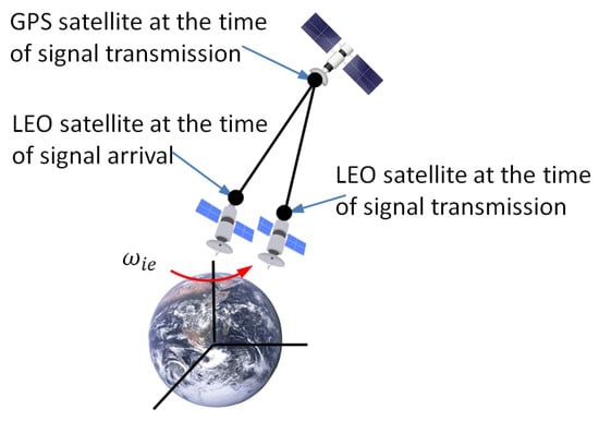
Figure 1.
Effect of Earth rotation on range calculation.
When the user processes a pseudorange and pseudorange rate measurement, the satellite position at the time of transmission must be used. During the time it takes the signal to propagate to the user’s antenna, the ECEF coordinate frame rotates slightly by an amount that is determined by the Earth’s rotation rate and the signal propagation time. To achieve complete accuracy in the GPS position and velocity fix, this small amount of rotation must be computed and compensated. Thus, the convenience of an ECEF frame calculation is combined with the accuracy of an ECI frame calculation by aligning ECI frame axes with ECEF frame axes at the time of signal arrival or transmission. For accurate processing of the GPS raw measurements, the GPS signal transit time is accounted for both pseudoranges and pseudorange rates in the navigation filter as well as the navigation processor for GPS navigation solution.
It is important to account for the signal transit time as the GPS satellite between the LEO satellite as a user distance generally changes over this interval. The LEO’s spaceborne GPS receiver obtains pseudorange measurements by multiplying its transit time measurements by the speed of light. The speed of light in free space is only constant in an inertial frame, where c = 299,792,458 m/s. In a rotating frame, such as ECEF, the speed of light varies. Consequently, the true range calculation is simplest in an ECI frame. Thus,
where is the position vector of the GPS satellite in the selected ECI coordinate system at the time of signal transmission, , and is the position vector of the LEO satellite in the selected ECI coordinate system at the time of signal arrival, .
As the user position is computed with respect to the Earth and the GPS interface standard gives formulas for computing the satellite position in ECEF coordinates, it is convenient to compute the range in an ECEF frame [7]. However, this neglects the rotation of the Earth during the signal transit time, causing the range to be overestimated or underestimated as illustrated in Figure 1. To compensate for this, a correction should be applied. The convenience of an ECEF frame calculation can be combined with the accuracy of an ECI frame calculation by aligning the ECI frame axes with the ECEF frame axes at the time of signal arrival or transmission [19]. The position vector of the LEO satellite at the time of signal arrival is given by
where I denotes an ECI frame synchronized with a corresponding ECEF frame, where e denotes the time of signal arrival. However, the position vector of the LEO satellite at the time of signal arrival needs to be expressed by [7]
where the rotation matrix that transforms the ECEF frame to the ECI frame at the time t is given by
where the rotation matrix that transforms the ECEF frame to the ECI frame at the time is given by
Since the true range between the GPS satellite and receiver is given as
where c is the speed of light. Substituting this into Equation (18), the rotation matrix can be alternatively expressed as a function of the signal propagation time:
The range is then be expressed by
The direction from which a satellite signal arrives at the user antenna may be described by a unit vector. The line-of-sight unit vector from the LEO antenna, a, to GPS satellite, s, resolved about the ECI frame axes, is given by [7]
The corresponding ECEF frame line-of-sight vector is given by [7]
The range rate is the rate of change of the range. Differentiating Equation (23),
Alternatively, using the ECEF-frame LOS unit vector and accounting for the Earth’s rotation, the range rate can be expressed as [7]
Thus, both corrections on pseudoranges and pseudorange rates are essential for high-precision GPS positioning, especially in dynamic applications such as aircraft navigation, spacecraft tracking, and geodetic surveying.
2.5. Navigation Processor in a Dual-Frequency Spaceborne GPS Receiver
As the kinematic solutions for pseudoranges and pseudorange rates, the least-squares estimation method is widely used to solve for the receiver’s position and velocity by minimizing the error between measured and predicted observations. This subsection describes how a least-squares estimation method as a GPS navigation processor calculates a LEO satellite position and velocity and calibrates the receiver clock errors using ionosphere-error-free pseudoranges and pseudorange rates correcting signal time delay. The ranging processor outputs measurements for all the satellites tracked at a common time of signal arrival. When it does not apply corrections for an LEO satellite clock errors and the ionosphere propagation delays, these corrections should be applied by the navigation processor. The navigation solutions are obtained by solving the above equations with pseudorange and pseudorange rate measurements from at least four satellites. When an ECEF frame is used, most navigation solution processors make use of an estimated or predicted pseudorange and pseudorange rate given by
where are the estimated satellite position and velocity in the ECEF frame, obtained from the navigation message; and are the navigation processor’s estimates of the LEO antenna position and velocity; and are the estimates of the receiver clock offset and drift; is the line-of-sight vector obtained from the estimated GPS satellite and LEO positions; and is the estimated time of signal transmission. This is determined by
Then, the estimated range and range rate are
and
When the ECEF frame is used, the least-squares estimation solution is
where and are the mth ionosphere-error-free combination psueudoranges and pseudorange rates in Equations (12) and (13), and
where
It is important to note that the pseudorange measurement is independent of the user velocity and clock drift, whereas the pseudorange rate is not affected by the clock offset. The sensitivity of the pseudorange rate to user position is minimal; specifically, a 1-m position error has an equivalent effect to a velocity error of approximately m/s. Consequently, the partial derivative term is typically neglected in practice [7]. Furthermore, the navigation solution is commonly computed without explicitly modeling the signal propagation delay. As a result, the attitude transformation matrix in Equations (26) and (27) is approximated as the identity matrix when applied to the least-squares estimation solution in Equation (31). This simplification significantly reduces computational complexity while maintaining acceptable estimation accuracy.
2.6. Measurement Model
The measurement model of the EKF is given by
where is the observation vector obtained from the navigation solutions provided by the space-borne GPS receiver at every sampling rate.
Since the GPS navigation solutions are used as the observations in the EKF, the observation assuming no noise, , and its partial derivative at the time, , can be obtained directly from the inertial coordinate system:
where is the identity matrix and is the null matrix. The noise vector , which represents the random noise errors of the measurements is modeled by
and the observation error covariance matrix is given by [3]
where are the chosen standard deviations of the position, velocity, clock offset/bias, and drift, respectively, obtained by the least-squares estimation solutions using the RMSE values.
2.7. State Transition Matrix
Another potential source of computer burden is the evaluation of the transition matrix arising from the partial derivatives of equations of the orbital motion. It was noticed that more complex computation, e.g., including (geopotential coefficient representing the Earth oblateness) or other effects, does not lead to significant advantages in real-time algorithms [1,3,16]. While purely Keplerian state transition matrices may cause slow convergence of iterated differential correction methods for orbit determination, the incorporation of the lowest-order zonal gravity field perturbation already provides an acceptable minimum model. The differential equation of the state transition matrix [17] is given by
where the nonlinear equation is given by
The Jacobian matrix in Equation (40) is defined by
where is the gradient matrix of the total acceleration with respect to position , including central gravity , perturbation, and centrifugal effects; is the gradient of the Coriolis acceleration with respect to velocity . The gradient matrix is decomposed as
where the gradient matrix including the central force is given by
The perturbation is derived from the gradient of the disturbing function [20]:
yielding the perturbation acceleration:
The Jacobian matrix consists of the derivatives of these components with respect to . The Coriolis effect gradient with respect to velocity is
where
The gradient matrix of the centrifugal acceleration with respect to the position is given by
The gradient matrix of the Coriolis acceleration with respect to the velocity is given by
Finally, the state transition matrix is computed by numerically integrating from to with initial condition for sequential computational algorithm.
3. Extended Kalman Filter
The extended Kalman filter (EKF) provides a minimum-variance estimate of the system state by incorporating statistical information from both the dynamic model and the available observations. The EKF algorithm consists of two main steps: the time update (prediction) and the measurement update (correction). In the time update phase, the state estimate and the associated covariance matrix are propagated forward using the nonlinear system dynamics. In this research, the predicted state at time and the corresponding state transition matrix are obtained by numerically integrating the equations of motion and the associated variational equations:
where denotes the nonlinear system dynamics, is the state transition matrix, which relates the state deviation between and , and is the covariance of the process noise, which is a measurement of the error between the reference state and the true state arising from imperfect modeling.
In the case that navigation solutions are used as observations, the computed observation and its partial derivative at time , as well as , can be obtained directly.
In the measurement update step, the predicted state and covariance are corrected using new GPS measurements at time . The Kalman gain , which weights the correction based on the predicted uncertainty and observation accuracy, is given by
where is the measurement noise covariance matrix, typically assumed to be diagonal for uncorrelated observations. The updated estimated state vector and the update covariance are given by
where and are the measurement and the measurement residuals at epoch for the position and velocity as the GPS navigation. The observation noise is the discrete measurement noise covariance, which is basically a measurement weight matrix. To be precise, the measurements should be uncorrelated, in which case the measurement noise covariance is diagonal.
4. Simulation Overview
This section provides an overview of the numerical simulations conducted for GPS measurement generation, navigation solution computation, and orbit estimation. The proposed RTOD algorithm is evaluated through a four-step simulation process as described below.
Step 1: Simulation of LEO satellite and GPS constellation. The first step involves generating the ephemerides of a low Earth orbit (LEO) satellite and defining the simulation duration. These inputs are utilized in Satellite Tool Kit (STK) using the High Precision Orbit Propagator (HPOP) and a GPS constellation propagator to simulate the LEO satellite and the GPS satellites. The resulting trajectories are expressed in both ECI and ECEF reference frames, allowing a direct comparison between the estimated orbit from the EKF and the reference (truth) orbit.
Step 2: GPS measurement simulation. In this step, GPS measurements are simulated for the LEO satellite using the visible GPS constellation. The MATLAB Navigation Toolbox function pseudoranges is used to generate pseudoranges and pseudorange rates. This function requires the receiver’s position in geodetic coordinates (latitude, longitude, altitude), velocity in the local navigation frame, and the GPS satellites’ positions and velocities in the ECEF frame. To meet these requirements, the LEO satellite’s ECEF position and velocity are transformed accordingly. The xyz2llh.m function is used to convert ECEF coordinates into geodetic coordinates, while ecef2ned.m transforms the velocity vector into the North-East-Down (NED) local frame, as illustrated in Figure 2. It is important to note that the pseudoranges function does not simulate ionospheric delays or their temporal variation, both of which are significant error sources in real-world GPS measurements. To address this, the Klobuchar model is implemented to simulate ionospheric delays and delay rates. These modeled errors are then superimposed onto the generated pseudoranges and pseudorange rates to better reflect realistic signal propagation effects in LEO conditions.
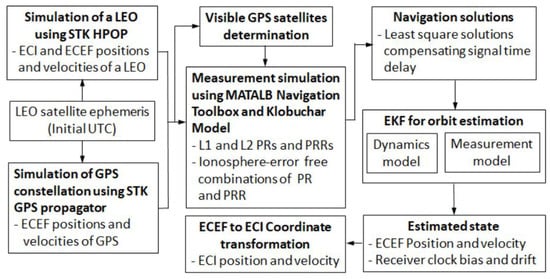
Figure 2.
Overall simulation flow including the interaction between the GPS measurement simulation and the RTOD algorithm for the LEO satellite.
Step 3: Computation of GPS navigation solutions. Using the simulated pseudoranges and pseudorange rates, GPS navigation solutions are computed through least-squares estimation, resulting in kinematic position and velocity solutions. Two sets of navigation solutions are produced: one that includes ionospheric delay compensation (enhanced GPS solution), and one that does not (baseline solution). These solutions serve as inputs for the subsequent orbit estimation phase.
Step 4: Orbit estimation ising EKF. In the final step, the EKF-based orbit estimation is conducted in the ECEF frame using both GPS navigation solutions. The orbit estimated from the enhanced GPS navigation solution is further transformed into the ECI frame for comparative analysis. The complete simulation process, including the interaction between GPS measurement generation and the RTOD algorithm, is depicted in Figure 2.
5. Simulation Results
This section presents numerical simulations to validate the proposed RTOD algorithm using two sets of simulated GPS navigation solutions. The first set is obtained without GPS signal delay corrections, while the second set incorporates these corrections. For orbit estimation, the EKF utilizes least-squares estimation solutions of simulated pseudoranges and pseudorange rates as measurement inputs. The simulation spans 24 h with a 10-s time step, starting from 15 July 2022, at 00:00:00 UTC.
5.1. GPS Constellation, LEO and Measurements
This subsection presents simulation results characterizing the GPS constellation, the LEO satellite trajectory, and the corresponding measurement data. Figure 3 and Figure 4 depict the GPS constellation and the LEO orbit in both the EC and ECEF reference frames. The visibility of GPS satellites from the LEO satellite is assessed by computing elevation angles. Based on these calculations, the number of visible GPS satellites and the associated dilution of precision (DOP) values are determined. Figure 5 shows that the number of visible satellites varies between 7 and 14, ensuring sufficient visibility for positioning. Figure 6 illustrates the geometric (GDOP), position (PDOP), horizontal (HDOP), and vertical (VDOP) dilution of precision. Although elevated DOP values are observed briefly near 11.5 h, the overall values remain within acceptable bounds, indicating favorable GPS observation geometry for LEO navigation.
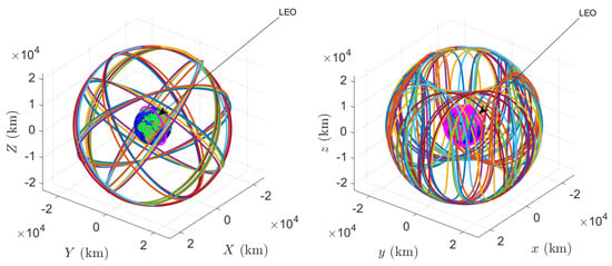
Figure 3.
GPS constellation and a LEO in the ECI (left) and ECEF (right) frames.
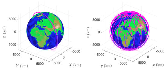
Figure 4.
A LEO in the ECI (left) and ECEF (right) frames.
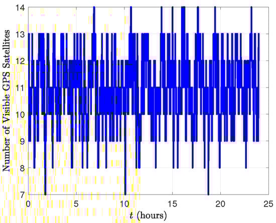
Figure 5.
Number of visible GPS satellites.
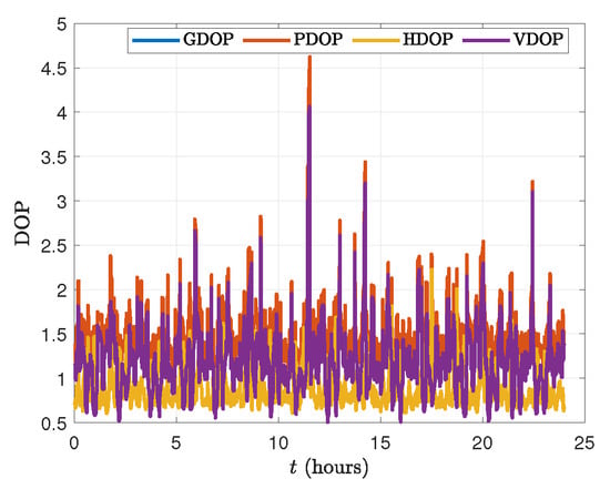
Figure 6.
Dilution of precision (DOP).
Figure 7 and Figure 8 present the differences between the PR and the true ranges (R), and the difference between the PRR and the true range rate () for both the L1 frequency measurements and the IEFC measurements, respectively. The left of Figure 7 shows the PR and PRR errors when signal time delays are not compensated, while the right of Figure 7 shows the PR and PRR errors when signal time delays are compensated. Though signal time delays are compensated in the right of Figure 7, they show very similar errors both in PR and PRR. This is due to the fact that the ionosphere error is more dominant than the effect of signal time compensation. On the other hand, the effect of signal time compensation is clear for the IEFC measurements in Figure 8. The left of Figure 8 shows the PR and PRR errors when signal time delays are not compensated, while the right of Figure 8 shows the PR and PRR errors when signal time delays are compensated. Unlike the PR and PRR errors in Figure 7, the PR and PRR errors in Figure 8 are reduced when signal time delays are compensated for the IEFC measurements. The comparison clearly demonstrates that accounting for signal propagation delays significantly reduces the errors in PR and PRR.
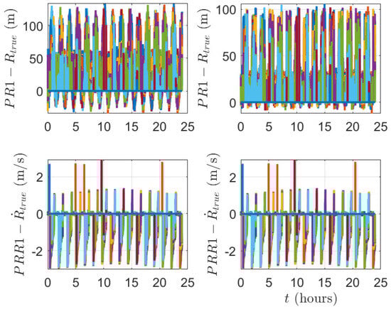
Figure 7.
Pseudorange and pseudorange rate errors of L1 frequency measurements.
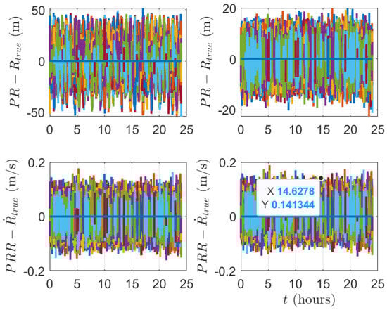
Figure 8.
Pseudorange and pseudorange rate errors of ionosphere-error-free combination measurements.
Figure 9 illustrates the variation in GPS signal transit times, ranging from approximately 0.0641 s to 0.874 s. These variations underscore the necessity of compensating for signal propagation delays in range calculations to enhance measurement accuracy. The observed reduction in the discrepancies between the raw pseudoranges and the computed geometric ranges confirms the effectiveness of this correction in improving orbit determination precision for low-Earth-orbit satellites. Additionally, Figure 10 shows the true position and velocity states in the Earth-centered, Earth-fixed frame, generated by the high-precision orbit propagator in the Satellite Tool Kit. These true states serve as a reference for evaluating the accuracy of the computed and estimated states obtained through the least-squares estimation method and the extended Kalman filter, as discussed in the subsequent subsections.
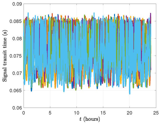
Figure 9.
GPS signal transit time.
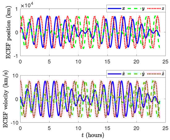
Figure 10.
True ECEF positions and velocities.
5.2. GPS Navigation Solutions
This subsection presents two GPS solutions derived using ionosphere-free pseudoranges and pseudorange rates, computed through the least-squares estimation method, with an emphasis on the impact of signal transit time compensation. Figure 11 illustrates the resulting position and velocity errors from two computational approaches.
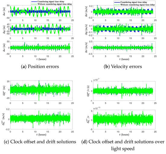
Figure 11.
Least-squares estimation solutions using the pseudoranges and pseudorange rates.
The estimation errors are obtained by subtracting the least-squares estimation solutions from the referenced Earth-centered, Earth-fixed truth positions and velocities. Green markers represent Case 1, in which signal transit time is not corrected, while blue markers indicate Case 2, which incorporates compensation for signal propagation time and Earth’s rotation. In Case 2, the correction accounts for the satellite’s motion during the signal’s travel time, resulting in visibly improved accuracy in both position and velocity estimation. Figure 11c,d depict the estimated receiver clock offset and drift for both cases, shown in standard form and normalized by the speed of light, respectively. These estimates remain nearly identical across both cases, suggesting that signal transit time correction primarily affects position and velocity estimation, with minimal influence on receiver clock estimation. Table 1 summarizes the RMSE values for each case. As expected, Case 2 yields significantly reduced RMSE values in position components, especially in the in-track and cross-track directions, while the velocity errors remain similar between the two cases. This outcome confirms the benefits of incorporating Earth rotation effects during signal propagation in the least-squares estimation formulation given by Equation (31). To assess radial, in-track, and cross-track position errors in the radial, in-track, and cross-track (RIC) frame, the estimated positions are first transformed from the Earth-centered, Earth-fixed frame to the Earth-centered inertial frame using Equation (4), and subsequently to the RIC frame using the rotation matrix:
This transformation enables the decomposition of orbital errors into radial, in-track, and cross-track directions. The findings provide clear evidence that incorporating Earth rotation effects into the least-squares estimation process substantially improves the accuracy of real-time onboard orbit determination using GPS measurements.

Table 1.
Least-squares estimation solution results for GPS navigation solutions (RMSE).
5.3. Orbit Estimation Results
In the orbit determination simulations, two distinct GPS navigation solutions were used as measurement inputs to the extended Kalman filter (EKF), differing by whether signal transit time delays were accounted for. These delays, discussed in the previous subsection, arise due to the finite speed of light and Earth’s rotation during signal propagation. Accordingly, two EKF estimation scenarios were examined: Case 1: EKF using a GPS navigation solution that neglects signal transit time. Case 2: EKF using a GPS navigation solution that incorporates signal transit time compensation. To evaluate estimation performance, position and velocity errors were computed by comparing the estimated states to the simulated Earth-centered, Earth-fixed (ECEF) truth data generated using a high-precision propagator. The initial state errors for the EKF were set as follows: The position error is m, the velocity error is m/s, the receiver clock offset/bias error is −100 m, and the clock drift error is 1 m/s, ensuring that the RMSE performance of the EKF could be compared with that of the raw GPS navigation solutions. The initial error covariance matrix that reflects the variances of the corresponding state elements is defined in Equation (10) and is expressed as
The specific numerical values adopted for are listed in Table 2.
Table 2.
Numerical values for the initial error covariance matrix, .
The process noise covariance that reflects the uncertainty in the dynamic model used during the prediction step of the EKF in Equation (52) follows the same state ordering:
where is the noise covariance matrix of the empirical accelerations defined as
where is a steady-state variance of the corresponding empirical acceleration component, , and is the three-dimensional identity matrix. The numerical values for are summarized in Table 3.
Table 3.
Numerical values for the process noise covariance matrix, .
To properly incorporate the two distinct GPS navigation solutions into the EKF, appropriate measurement error covariance matrices were selected to reflect their respective accuracy levels. The correct tuning of is crucial for achieving optimal filter performance. Two configurations were employed:
where in Equation (62a) corresponds to the solution without signal transit time correction, and in Equation (62b) corresponds to the solution with the correction (higher accuracy).
Figure 12 presents the measurement residuals for position and velocity in both estimation cases, serving as indicators of filter convergence. In Case 1, where signal transit time is neglected, the position residuals are bounded within approximately m, while in Case 2, with signal time delay compensation, the bounds are reduced to approximately m. Velocity residuals remain within m/s for both cases. The RMSE values of the position measurements are 13.875 m for Case 1 and 9.185 m for Case 2. For velocity measurements, the RMSE values are 0.095 m/s and 0.067 m/s, respectively. These reductions highlight the benefits of accounting for signal transit time in pseudorange measurements.
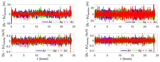
Figure 12.
Measurement residuals in the EKF for Case 1 and Case 2.
Figure 13 shows the position and velocity estimation errors along with their associated confidence bounds from the EKF covariance matrix for both cases. For Case 1, position errors are bounded within m and velocity errors within m/s. Case 2 shows improved performance, with position and velocity errors bounded within approximately m and m/s, respectively. In both cases, all estimation errors remain within the bounds, confirming the consistency of the EKF.
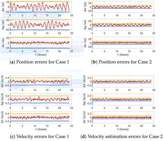
Figure 13.
Position, velocity estimation errors, and bounds from the EKF.
Table 4 presents the RMSE results for both cases. Position RMSE values in Case 2 are significantly lower, especially in the in-track and cross-track directions. Velocity RMSE values are similar across both cases, reflecting consistent velocity estimation quality.
Table 4.
EKF state estimation results using the two distinct GPS navigation solutions (RMSE).
Figure 14 shows the position and velocity estimation errors in the RIC frame for Case 2. Errors remain less than m for position and m/s for velocity in all three components.
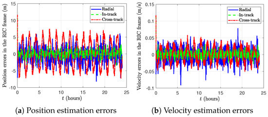
Figure 14.
Position and velocity estimation errors in the RIC frame for Case 2 (singal time delay compensation).
Figure 14 illustrates the position and velocity estimation errors in the RIC frame for Case 2. The position estimation errors remain within ±10 m, while the velocity estimation errors are bounded within ±0.06 m/s in the radial, in-track, and cross-track directions. Figure 15 shows the norms of the position and velocity estimation errors, along with the square roots of the trace of the corresponding submatrices of the error covariance matrix, , for Case 2. The convergence of the extended Kalman filter (EKF) is confirmed by the decreasing trend in the square roots of the trace of the error covariance matrix over time, indicating improved confidence in both position and velocity estimates. This performance reflects the effectiveness of the filter tuning, particularly in modeling the empirical accelerations and process noise characteristics. The results affirm the EKF’s capability to maintain high estimation accuracy despite limited onboard measurements.
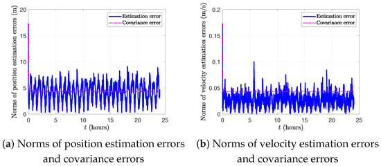
Figure 15.
Norms of position and velocity estimation errors and covariance errors for Case 2.
Table 5 presents a comparison between the EKF estimation results and the GPS navigation solution for Case 2. The EKF consistently yields smaller RMSE values compared to the standalone GPS navigation solution, demonstrating improved estimation accuracy. This enhanced performance is attributed to the EKF’s optimal fusion of dynamic models and measurement updates. Furthermore, the EKF maintains superior estimation accuracy even when signal transit time is accounted for in the least-squares estimation solutions, as described in Equation (31). These results highlight the advantage of the EKF framework in incorporating both physical models and measurement uncertainties and using ionosphere-free error combination measurements from a dual-frequency spaceborne GPS receiver to produce reliable and precise state estimates.
Table 5.
Comparison of the EKF estimation results with the GPS navigation solutions (RMSE).
6. Conclusions
This study presents an enhanced real-time onboard orbit determination method for low-Earth-orbit (LEO) satellites, incorporating GPS signal propagation delay compensation using dual-frequency measurements from a dual-frequency spaceborne receiver. The proposed approach is built upon a reduced-dynamic orbit determination (RDOD) framework and a predictive correction model to mitigate signal delays, leveraging ionosphere-free combinations of pseudorange and pseudorange rate measurements. To generate realistic measurement data, a GPS measurement simulator was developed using the Satellite Tool Kit’s high-precision orbit propagator (HPOP) and a GPS constellation model. Synthetic dual-frequency measurements were produced with MATLAB’s Navigation Toolbox, and the Klobuchar model was employed to simulate ionospheric delays and their rates, which were then added to the raw measurements to enable realistic signal delay modeling. The accuracy of GPS navigation solutions was significantly improved by correcting for signal travel time and Earth rotation effects. These corrected solutions were computed using a least-squares estimation method and subsequently integrated into the extended Kalman filter (EKF) for real-time orbit estimation. The EKF was shown to maintain stable performance with a 10-s sampling rate using a fourth-order Runge–Kutta integrator, even under simplified dynamic modeling. The inclusion of the perturbation in the state transition matrix contributed to model consistency without increasing computational complexity.
Simulation results confirm that the proposed Earth-centered, Earth-fixed (ECEF)-based algorithm outperforms conventional methods that neglect signal delay effects. Over a one-day simulation, the method achieved root-mean-squared errors of 3.34 m in position and 0.02 m/s in velocity, satisfying the 10-m onboard orbit accuracy requirement. The filter also successfully estimated the GPS receiver’s clock bias and drift, ensuring robustness in high-dynamic environments. Overall, this work demonstrates that combining ECEF-based estimation, reduced-dynamic filtering, dual-frequency ionosphere-free measurement processing, and GPS signal delay compensation offers a practical and accurate solution for real-time autonomous orbit determination in LEO satellite missions. Finally, to stimulate future research, the incorporation of more accurate and comprehensive gravitational field models is recommended to further enhance orbit determination fidelity.
Author Contributions
Conceptualization, D.L.; Methodology, D.L.; Software, D.L. and S.S.H.; Validation, D.L.; Formal analysis, D.L.; Investigation, D.L.; Resources, D.L.; Writing—original draft, D.L.; Writing—review and editing, D.L. and S.S.H.; Visualization, D.L.; Supervision, D.L.; Project administration, D.L. All authors have read and agreed to the published version of the manuscript.
Funding
This research received no external funding.
Data Availability Statement
There is no new data created in this manuscript.
Conflicts of Interest
Author Daero Lee was employed by the company Solid Aerospace. The remaining authors declare that the research was conducted in the absence of any commercial or financial relationships that could be construed as a potential conflict of interest.
References
- Chiaradia, A.P.M.; Gill, E.; Montenbruck, O.; Kuga, H.K.; Prado, A. Algorithms for On-Board Orbit Determination Using GPS OBODE-GPS. In Proceedings of the DLR-GSOC TN 00-04. 2000. Available online: https://elib.dlr.de/11320/ (accessed on 20 April 2025).
- Yoon, J.C.; Lee, B.S.; Choi, K.H. Spacecraft orbit determination using GPS navigation solutions. Aerosp. Sci. Technol. 2000, 4, 215–221. [Google Scholar] [CrossRef]
- Gomes, V.M.; Kuga, H.K.; Chiaradia, A.P.M. Real time orbit determination using GPS navigation solution. J. Braz. Soc. Mech. Sci. Eng. 2007, 29, 274–278. [Google Scholar] [CrossRef]
- Yu, Z.; You, Z. Real-time onboard orbit determination using GPS navigation solutions. In Proceedings of the 2011 First International Conference on Instrumentation, Measurement, Computer, Communication and Control, Beijing, China, 17–20 October 2011; pp. 949–952. [Google Scholar]
- Aghav, S.T.; Gangal, S.A. Simplified orbit determination algorithm for low earth orbit satellites using spaceborn GPS navigation sensor. Artif. Satell. 2014, 49, 81–99. [Google Scholar] [CrossRef]
- Hegarty, C.; Kaplan, E. Understanding GPS: Principles and Applications, 2nd ed.; Artech House: New York, NY, USA, 2005; pp. 379–454. [Google Scholar]
- Groves, P.D. Principles of GNSS, Inertial, and Multisensor Integrated Navigation Systems, 2nd ed.; GNSS Technology and Applications; Artech House: New York, NY, USA, 2013; pp. 339–341. [Google Scholar]
- Misra, P.; Enge, P. Global Positioning System: Signals, Measurements, and Performance, 2nd ed.; Ganga-Jamuna Press: Nanded, India, 2006; pp. 115–128. [Google Scholar]
- Chiaradia, A.P.M.; Kuga, H.K.; de Almeida Prado, A.F.B. Onboard and real-time artificial satellite orbit determination using GPS. Math. Probl. Eng. 2013, 2013, 571–576. [Google Scholar] [CrossRef]
- Hu, W.; Farrell, J.A. Derivation of the Sagnac (Earth-rotation) correction and analysis of its accuracy for GNSS applications. J. Geod. 2024, 98, 102. [Google Scholar] [CrossRef]
- Montenbruck, O.; Gill, E. Ionospheric correction for GPS tracking of LEO satellites. J. Navig. 2002, 55, 293–304. [Google Scholar] [CrossRef]
- Hofmann-Wellenhof, B.; Lichtenegger, H.; Wasle, E. GNSS—Global Navigation Satellite Systems; SpringerWien: New York, NY, USA, 2008; pp. 113–126. [Google Scholar]
- Chiaradia, A.; Kuga, H.; Prado, A. Single frequency GPS measurements in real-time artificial satellite orbit determination. Acta Astronaut. 2003, 53, 123–133. [Google Scholar] [CrossRef]
- Leick, A.; Rapoport, L.; Tatarnikov, D. GPS Satellite Surveying; John Wiley & Sons, Inc.: Hoboken, NJ, USA, 2015; pp. 257–399. [Google Scholar]
- Gaylor, D.E.; Page, R.G.; Bradley, K.V. Testing of the java astrodynamics toolkit propagator. In Proceedings of the AIAA/AAS Astrodynamics Specialist Conference, Keystone, CO, USA, 21–24 August 2006; pp. 2072–2082. [Google Scholar]
- Montenbruck, O.; Gill, E. Satellite Orbits: Models, Methods and Applications, 1st ed.; Springer: Berlin/Heidelberg, Germany, 2000; pp. 159–192, 217–219, 241–242. [Google Scholar]
- Tapley, B.; Schutz, B.; Born, G.H. Statistical Orbit Determination; Elsevier Academic Press: San Diego, CA, USA, 2004; pp. 194–212, 230–233, 505–510. [Google Scholar]
- Marshall, J.A.; Luthcke, S.B. Erratum-modeling radiation forces acting on Topex/Poseidon for precision orbit determination. J. Spacecr. Rocket. 1994, 31, 535–536. [Google Scholar] [CrossRef]
- DiEsposti, R. Time-dependency and coordinate system issues in GPS measurement models. In Proceedings of the 13th International Technical Meeting of the Datellite Division of the Institute of Navigation (ION GPS 2000), Salt Lake City, UT, USA, 19–22 September 2000; pp. 1925–1929. [Google Scholar]
- Vallado, D.A. Fundamentals of Astrodynamics and Applications, 4th ed.; Microcosm Press: Portland, OR, USA, 2015; pp. 593–595. [Google Scholar]
Disclaimer/Publisher’s Note: The statements, opinions and data contained in all publications are solely those of the individual author(s) and contributor(s) and not of MDPI and/or the editor(s). MDPI and/or the editor(s) disclaim responsibility for any injury to people or property resulting from any ideas, methods, instructions or products referred to in the content. |
© 2025 by the authors. Licensee MDPI, Basel, Switzerland. This article is an open access article distributed under the terms and conditions of the Creative Commons Attribution (CC BY) license (https://creativecommons.org/licenses/by/4.0/).