Article

Engineering-Oriented Layout Optimization and Trade-Off Design of a 12U CubeSat with In-Orbit Validation

1
Research Center of Satellite Technology, Harbin Institute of Technology, Harbin 150001, China
2
State Key Laboratory of Micro-Spacecraft Rapid Design and Intelligent Cluster, Harbin Institute of Technology, Harbin 150001, China
3
Department of Astronautical Science and Mechanics, Harbin Institute of Technology, Harbin 150001, China
4
Department of Electrical Engineering, Harbin Institute of Technology, Harbin 150001, China
*
Author to whom correspondence should be addressed.
Aerospace 2025, 12(6), 506; https://doi.org/10.3390/aerospace12060506
Submission received: 8 May 2025 / Revised: 30 May 2025 / Accepted: 2 June 2025 / Published: 3 June 2025
(This article belongs to the Special Issue Space System Design)

Abstract

The extensive application of CubeSats in fields such as communication, remote sensing, and scientific exploration highlights their significant engineering value. With the growth of CubeSat dimensions towards 12U and beyond, their potential for engineering applications has further expanded. However, strict size constraints significantly limit the layout design space, causing difficulties in satellite system design through multiple iterations. To address these practical issues, this paper proposes an engineering-oriented layout optimization and trade-off design approach tailored specifically for 12U CubeSats, employing a hybrid optimization framework combining GRASP and NSGA-III algorithms. The proposed methodology facilitates initial feasibility analysis, informed trade-off decisions during iterative design, and detailed optimization in later stages, thereby improving design efficiency and practicality. The proposed optimization systematically explores design compromises considering conflicting objectives such as mass properties, thermal management, and spacing constraints. The ASRTU Friendship MicroSat, a 12U CubeSat, serves as a case study, with in-orbit performance validating the proposed approach. Results demonstrate that the optimized layouts effectively address complex engineering constraints, enabling satellite design teams to successfully achieve optimized layout solutions in practical engineering applications.

1. Introduction

CubeSats, initially proposed in the late 1990s by Stanford University and California Polytechnic State University, began as educational platforms to engage students in spacecraft design and operations. Over two decades, CubeSats have rapidly evolved from educational missions into sophisticated platforms supporting diverse and complex missions including communications, Earth observation, climate monitoring, astronomy, and scientific research. This evolution has been driven largely by advancements in miniaturization technologies, cost-effective launch opportunities, and increased accessibility to space [1,2,3,4]. Initially standardized at the 1U and 3U form factors, CubeSats have expanded significantly to larger configurations such as 6U, 12U, 16U, and 24U. These larger CubeSats offer increased payload capacity and power, enabling more sophisticated missions typically performed by traditional larger satellites [5]. Notable examples include the Capstone mission, a 12U CubeSat developed by NASA and its partners to validate lunar orbit navigation technologies crucial for future lunar missions [6]. Additionally, the 6U MarCO satellites successfully accompanied NASA’s InSight lander to Mars, demonstrating unprecedented CubeSat capabilities in interplanetary communication and navigation [7]. Other prominent CubeSat missions include RainCube, a 6U CubeSat carrying miniaturized radar instrumentation to provide global precipitation measurements [8], and the 16U Lunar Flashlight mission designed to detect water ice at the Moon’s South Pole [9], exemplifying the versatility and growing importance of larger CubeSat platforms.
Despite their increased capabilities, CubeSats, particularly at 12U scale and above, encounter specific engineering constraints in their internal layout design. Firstly, stringent size constraints dictated by standardized deployment systems, such as CubeSat deployers aboard launch vehicles, severely restrict internal component arrangement, making efficient three-dimensional layouts challenging [10]. Achieving effective space utilization requires complex spatial planning and optimization. Secondly, CubeSats have limited resources for active thermal management systems, necessitating advanced passive thermal control strategies [11]. This limitation mandates careful internal component placement to ensure uniform thermal distribution, thereby avoiding thermal hotspots and enhancing system reliability. Thirdly, limited attitude control capability places increased importance on precisely managing mass properties, specifically minimizing rotational inertia and deviations in the center of gravity to maintain satellite stability and maneuverability [12]. Failure to optimize these aspects may significantly compromise mission performance and longevity. Lastly, the inherently customized nature of CubeSat missions frequently leads to iterative changes in component sizes and placements, demanding optimization algorithms that are highly adaptable and can dynamically accommodate evolving design requirements throughout the development process.
Satellite Layout Optimization Design (SLOD) significantly influences satellite performance, mission lifespan, and overall cost [13]. Traditionally, SLOD has been treated as a three-dimensional bin packing problem, an NP-hard challenge, solved by simplified geometric approximations and heuristic algorithms [14,15,16,17]. However, these traditional approaches usually fail to fully address the critical constraints and inherent complexities encountered in real satellite engineering. In recent years, advanced methods such as Differential Evolution (DE), Genetic Algorithms (GAs), and multi-objective optimization have been introduced to improve layout design [18,19,20,21]. Despite these advancements, modern techniques still face issues such as suboptimal space utilization and the neglect of essential constraints like thermal management, structural integrity, and mass balance, thereby reducing their practical applicability [22,23]. Furthermore, current methods often lack the flexibility to be seamlessly integrated into the various iterative scenarios typical of the satellite design process [24,25].
In response to these challenges, several studies have focused on three-dimensional component layout optimization. For instance, Liang et al. [26] proposed a decision support system that integrates multi-objective optimization with multi-attribute decision making for satellite layout. They developed a three-dimensional optimization model to minimize center-of-gravity offset and cross moments of inertia and introduced a space debris impact risk index. By coupling CAD software with optimization algorithms, their framework generates a Pareto front and uses a smart Pareto filter combined with the CCSD method to select the best trade-off solution. Similarly, Fakoor et al. [27] introduced the Spacecraft Component Adaptive Layout Environment (SCALE) for the three-dimensional layout of spacecraft subsystems. SCALE considers critical factors such as center of gravity, moments of inertia, thermal distribution, natural frequencies, and structural strength and integrates modeling, FEM, and optimization software to automatically generate optimal layout solutions. Case studies on telecommunication and remote sensing spacecraft show that SCALE significantly outperforms traditional baseline solutions. In addition to these three-dimensional layout approaches, several studies have focused on multi-objective optimization for satellite layout design. Zhang et al. [28] proposed an evolutionary multiagent framework based on a cooperative coevolutionary multi-objective model (CCMO-EMAS), where each agent optimizes a subpopulation and a collaborative mechanism, enhanced by an elite genetic algorithm, assembles complete solutions. Xu et al. [25] addressed the layout optimization for an orbital propellant depot by decomposing the problem into optimizing propellant tank arrangements and equipment positioning, ensuring that carrying capacity, the dry/wet ratio, and mass properties meet allowable limits. Moreover, Zheng et al. [29] developed a multi-objective methodology for satellite cabin layout optimization that incorporates space debris impact risk alongside mass properties. Finally, Cuco et al. [24] presented a multi-objective method for spacecraft equipment layouts, focusing on the distribution of electronic equipment on structural panels. By integrating CAD with optimization tools, their approach overcomes the limitations of experience-based placements through a comprehensive exploration of the conceptual design space.
Overall, traditional SLOD methods laid the foundation by simplifying the layout problem as a three-dimensional packing challenge, while subsequent advanced methods such as Differential Evolution (DE), Genetic Algorithms (GAs), and multi-objective optimization have made significant progress in tackling the complex constraints of modern satellite engineering. However, discrepancies between the outcomes of multi-objective optimization and practical engineering requirements, along with insufficient flexibility in the design process, still remain.
This paper proposes an engineering-oriented optimization approach specifically tailored for 12U CubeSats. Employing a hybrid optimization framework combining the Greedy Randomized Adaptive Search Procedure (GRASP) and Non-dominated Sorting Genetic Algorithm III (NSGA-III), this methodology effectively supports initial feasibility analyses, enables balanced decision-making throughout iterative design processes, and provides detailed refinement optimization in later stages. The proposed approach explicitly integrates practical engineering constraints, significantly enhancing adaptability and applicability in real-world satellite design scenarios. The effectiveness and practicality of this optimization approach are demonstrated through the ASRTU Friendship MicroSat project, validating the proposed method using actual in-orbit performance data and showcasing substantial improvements in layout design outcomes.

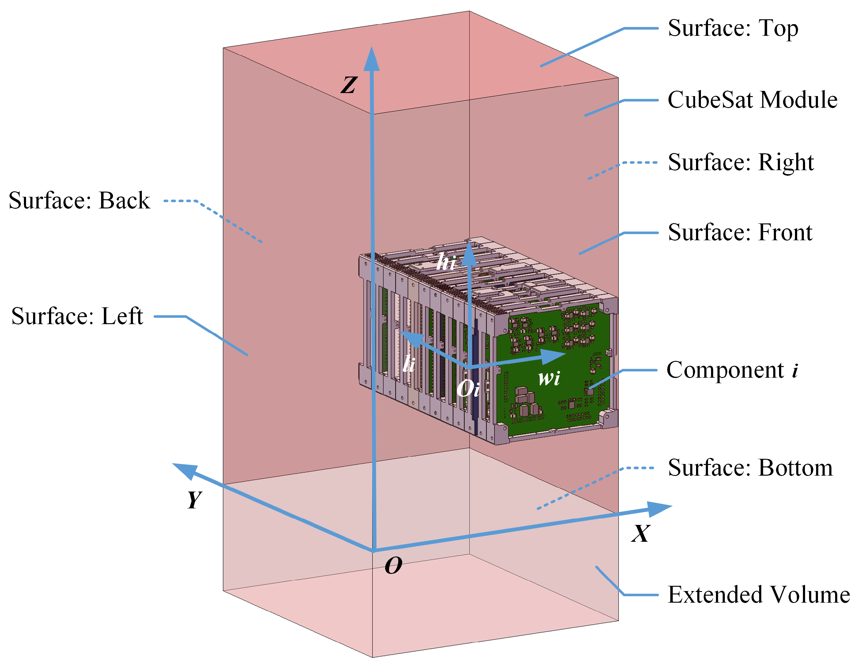
2. Mathematical Model for SLOD of Cubesats

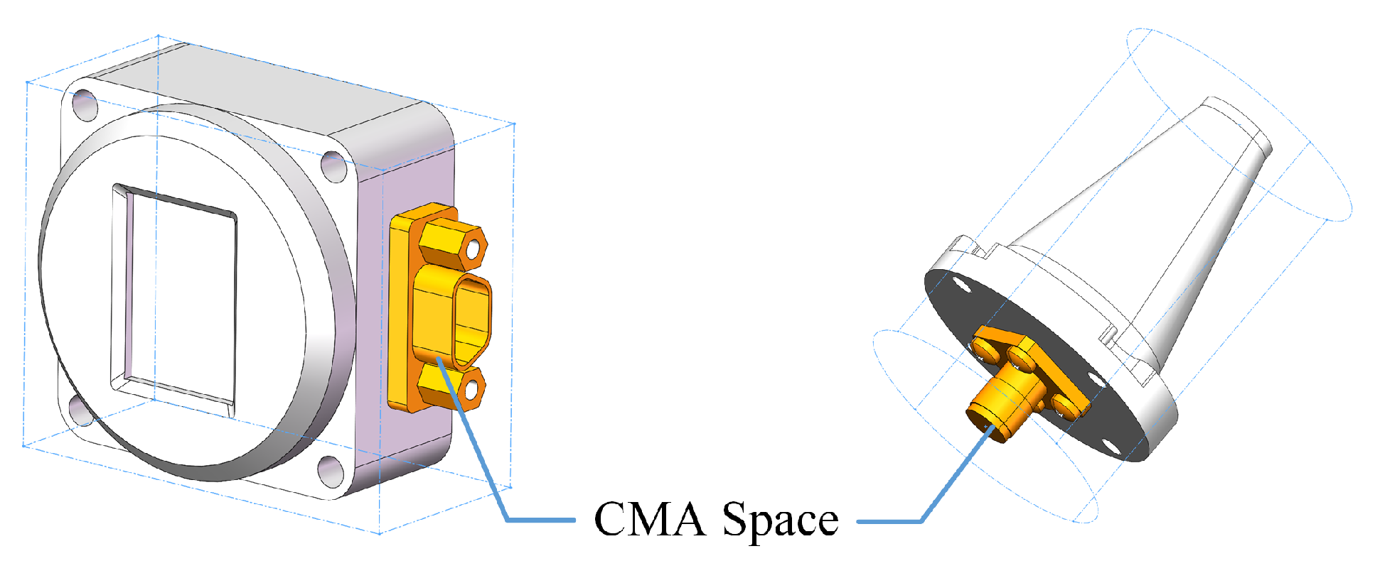
2.1. Key Features of CubeSats

CubeSats possess several key features that distinguish them from traditional satellite configurations and significantly impact their layout and design. These unique characteristics also present specific challenges for layout optimization.
One of the most critical features of CubeSats is that their dimensions are strictly constrained by design standards. Given their small volume and weight, the satellite components must adhere to stringent size requirements, which considerably limits the solution space for layout design. Furthermore, all components of a CubeSat are housed within a single satellite module, unlike traditional satellites that divide the layout into multiple compartments based on structural panels. Once the components are installed on their respective mounting surfaces, a unified calculation of interference among all components within the only module is necessary. The onboard components exhibit several notable characteristics. Most components are rectangular or can be enclosed within a rectangular bounding box, while others are better suited to a cylindrical bounding box. In addition, these components are subject to CMA (Compatibility, Maintainability, and Accessibility) constraints, which require careful design to ensure proper integration, ease of maintenance, and accessibility for wiring, cable routing, and other operational needs. It is crucial to ensure that there is no interference between the bounding volumes of different components and that all components are completely contained within the envelope of the satellite module. Another important aspect is that, due to resource limitations, CubeSats mainly rely on passive thermal control to maintain healthy in-orbit temperature environment. This imposes higher demands on the thermal distribution of the components, thereby necessitating that components are installed as close to the satellite’s structural panels as possible rather than being suspended in free space.
Considering these key features, the CubeSat module can be described as a cube, as shown in Figure 1. The satellite module consists of six mounting surfaces, front, back, left, right, top, and bottom, with additional extended volume at the bottom to simulate the unique Tuna Can space defined in CubeSat design standards.
To represent the dimensions and positions of the components, a bounding box method is adopted. Each component is described as either a rectangular or cylindrical box, as shown in Figure 2, while taking into account the CMA requirements. To address the computational complexity of three-dimensional space, the cubic bounding boxes are aligned with the satellite coordinate system.
This approach simplifies the complex engineering problem of CubeSat layout optimization into a mathematical model that can be efficiently solved, while still capturing the critical constraints and characteristics inherent in CubeSat design.

2.2. Assumption and Objectives

The CubeSat layout optimization relies on several simplifying assumptions to make the design problem tractable. The spacecraft’s structure is idealized as a rectangular cuboid, and each internal component is approximated by a rectangular or cylindrical bounding volume including CMA space. The mass of cables is omitted from the model; since they account for less than 5% of the total mass and are nearly uniformly distributed, their effect on the center of mass and moments of inertia is negligible. Additionally, any structural reinforcements or modifications required to accommodate components are assumed to have minimal impact on the CubeSat’s overall stiffness and dynamics, effectively preserving the characteristics of the standard frame.
Based on this simplified model, the layout is guided by multiple design objectives. The first is a strict non-interference requirement: all components must fit within the CubeSat’s volume without overlapping or colliding with one another or with the structural walls. The second objective is to optimize the satellite’s mass distribution by minimizing its principal moments of inertia and keeping the center of mass as close as possible to the geometric center. This mass-centric optimization enhances attitude stability and satisfies the typical CubeSat design specification that requires the center of gravity to lie within a few centimeters of the geometric center. In addition, thermal management considerations influence the component arrangement. To achieve a balanced thermal distribution, heat-generating components are placed on different surfaces of the CubeSat, ensuring that no single panel accumulates excessive heat. Moreover, certain subsystems must adhere to relative placement constraints; for instance, star sensors and gyroscopes should be put far away from reaction wheels to minimize disturbance torques. Such alignment guarantees that any vibrations or torques produced by the actuators do not significantly perturb the sensitive sensors, thereby improving the accuracy of attitude determination and control.
It is worth noting that some traditional satellite design factors are omitted in this CubeSat-focused layout design. In particular, no explicit constraint on the structure’s natural frequency is imposed. This simplification is justified due to the CubeSat’s standardized rigid structure and lack of large flexible appendages, ensuring that the fundamental frequency typically meets normal launch requirements. Because internal component placement has a negligible effect on the overall structural modes, the optimization can safely ignore natural frequency constraints and concentrate on the mission-specific layout objectives outlined above.

2.3. Mathematical Model

Let E = { e 1 , e 2 , , e n } represent the set of components of the CubeSat. Each component, e i , is described by several input parameters, including its name, shape type (box or cylinder), dimensions ( l i , w i , h i , and rotation angle θ i for boxes; radius r c i and length l c i for cylinders), mass ( m i ), allowed mounting surfaces ( F i ), centroid offset from the geometric center ( Δ c i ), power consumption ( P i ), position-fixed flags ( f i x e d _ x i , f i x e d _ y i , f i x e d _ z i , and f i x e d _ θ i ), and dimension-fixed flags ( f i x e d _ l i , f i x e d _ w i , and f i x e d _ h i for boxes; f i x e d _ r c i and f i x e d _ l c i for cylinders). The flags take Boolean values, where True indicates that the corresponding variable is constrained, and False indicates unconstrained.
The reference coordinate system O X Y Z is defined with the origin O at the bottom left corner of the internal envelope of the CubeSat module; the X-axis points from the left surface to the right surface, the Y-axis from the front surface to the back surface, and the Z-axis from the bottom surface to the top surface.
The design variable in CubeSat layout optimization is expressed as follows [23]:
L = { L i = ( x i , y i , z i , θ i , η i , s l i , s w i , s h i , s r c i , s l c i ) | i = 0 , 1 , , n 1 }
where ( x i , y i , z i ) denotes the centroid coordinates of component e i in O X Y Z , θ i is the rotation angle for box-shaped components, η i is the mounting surface index, ( s l i , s w i , s h i ) are size scaling factors for box-shaped components, and ( s r c i , s l c i ) are size scaling factors for cylindrical components. The proposed method balances five conflicting objectives, three to be minimized and two to be maximized, within a multi-objective framework.
According to the requirements, the objective of this problem is to find L by minimizing
f 1 ( L ) = V ( L )
f 2 ( L ) = C ( L )
f 3 ( L ) = I ( L )
f 4 ( L ) = T ( L )
f 5 ( L ) = D ( L )
subject to
g ( L ) = i = 0 n 1 j = i + 1 n Δ A i j | η i = η j = 0
where V ( L ) represents the total volume occupied by the components (to be maximized), C ( L ) denotes the centroid offset from the geometric center of the satellite (to be minimized), I ( L ) represents the sum of the three principal moments, T ( L ) represents the standard deviation of power(electric power consumption) distribution among six mounting surfaces (to be minimized), and D ( L ) represents the distance between sensors and actuators (to be maximized).
The constraint g ( L ) ensures no interference between components within the CubeSat module, where Δ A i j is the interference volume of two different components, where i = 0 represents the satellite envelope. Interference between components and the satellite module envelope is not considered explicitly, as this is inherently satisfied by the predefined ranges of the design variables.
The total volume of all components is defined as
V ( L ) = i = 1 n V i ,
where
V i = l i w i h i , if e i is box - shaped , π ( r c i ) 2 l c i , if e i is cylindrical .
The overall centroid of the satellite assembly, including all n internal components and the satellite structure, is given by
C = i = 1 n m i c i + m sat c sat i = 1 n m i + m sat ,
where m i and c i are the mass and centroid of component e i , and m sat and c sat are the mass and centroid of the satellite structure.
The centroid offset C ( L ) measures how far this overall centroid lies from the geometric center of the satellite’s bounding box. The envelope has the dimensions l 0 , w 0 , and h 0 (length, width, and height). Hence,
C ( L ) = ( C x l 0 2 ) 2 + ( C y w 0 2 ) 2 + ( C z h 0 2 ) 2 ,
where C = ( C x , C y , C z ) is as defined in (9).
Let
Δ r i = ( δ i 1 , δ i 2 , δ i 3 )
denote the displacement of the centroid of component e i from C . For a box-shaped component, the moment of inertia contributions along the principal axes are given by
I x x ( i ) = m i ( w i 2 + h i 2 ) 12 + m i δ i 2 2 + δ i 3 2 , I y y ( i ) = m i ( l i 2 + h i 2 ) 12 + m i δ i 1 2 + δ i 3 2 , I z z ( i ) = m i ( l i 2 + w i 2 ) 12 + m i δ i 1 2 + δ i 2 2 .
For cylindrical components, analogous formulas based on the corresponding dimensions are applied. The constant structural inertia is omitted because it does not affect optimization ranking:
I ( L ) = i = 1 N c I x x ( i ) + I y y ( i ) + I z z ( i ) .
The uniformity of the power (electric power consumption) distribution is measured by the standard deviation of the power density on the six mounting surfaces, F (top, bottom, front, back, left, and right), scaled by the average surface area. Let P f and A f denote, respectively, the total power and the area of surface f. We define the power density on surface f as
ρ f = P f A f ,
the mean power density as
ρ ¯ = 1 6 f F ρ f ,
and the average surface area as
A ¯ = 1 6 f F A f .
The uniformity metric for power distribution is then
T ( L ) = A ¯ 1 6 f F ρ f ρ ¯ 2 .
The aggregated separation between sensor and actuator components is defined as
D ( L ) = s S a A c s c a ,
where c s and c a are the centroids of the sensor and actuator components, respectively.
The overall optimization objective function is formulated as
φ ( L ) = i = 1 5 ω i f i ( L ) + λ g ( L ) ,
where the five objectives correspond to maximizing the component volume, minimizing the centroid offset, the moment of inertia, the power distribution standard deviation, and maximizing the sensor–actuator separation. Here, g ( L ) represents the single interference constraint function, and ω i and λ are the weighting and penalty coefficients, respectively.

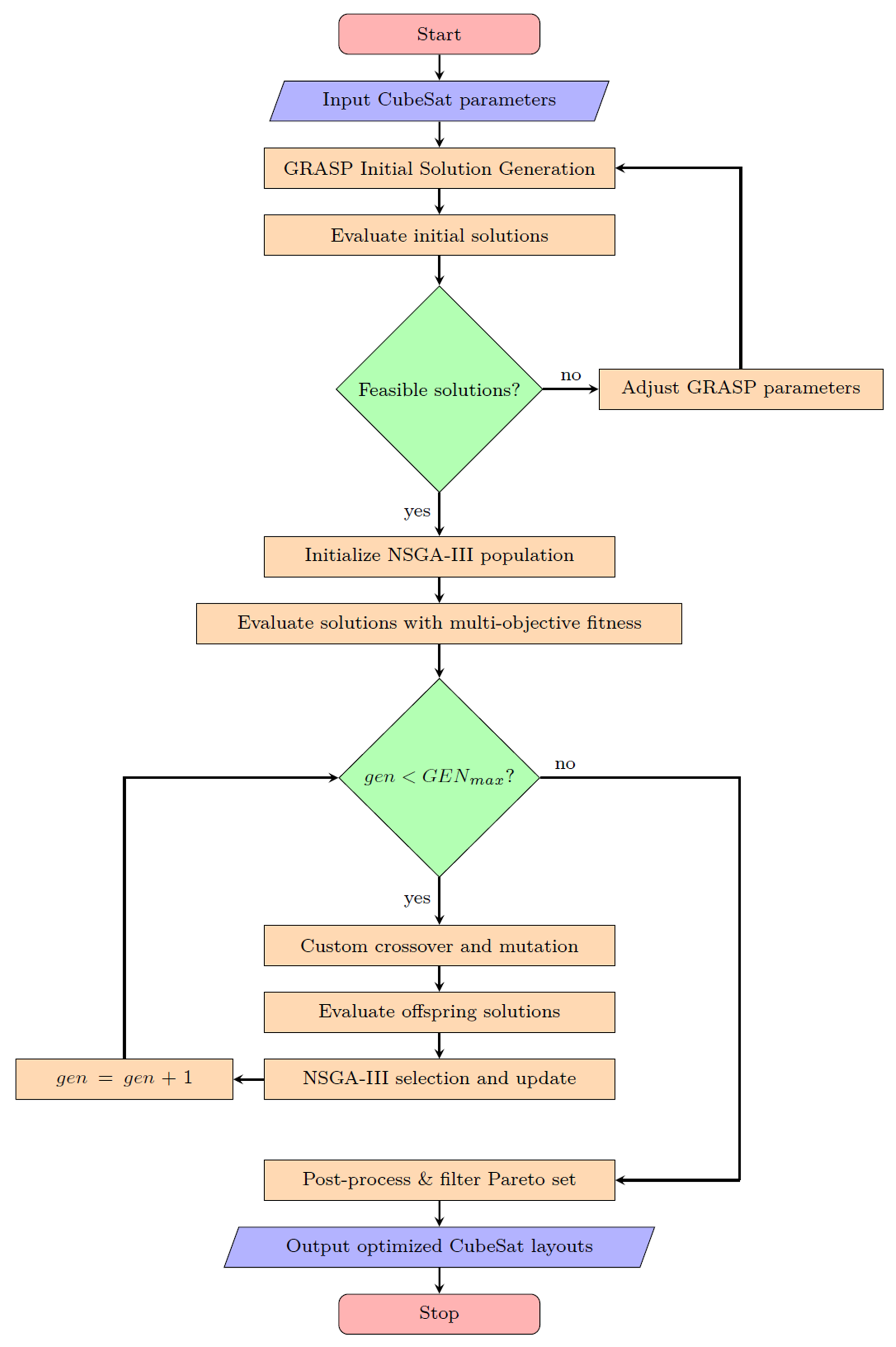
3. Hybrid Algorithm for CubeSat Layout Optimization and Trade-Off Design

This study presents a hybrid optimization approach for CubeSat layout design, aiming to provide direct engineering solutions under complex and conflicting constraints. Targeting the growing demand for larger CubeSats such as 12U, the method integrates the Greedy Randomized Adaptive Search Procedure (GRASP) [30] and Non-dominated Sorting Genetic Algorithm III (NSGA-III) [31] to perform layout optimization and trade-off analysis in a tightly constrained design space. By systematically balancing key factors, such as mass properties, thermal considerations, and interference avoidance, the proposed approach supports both early-stage feasibility evaluation and late-stage fine-tuning, enhancing overall engineering applicability and design efficiency.

3.1. Optimization Strategy

To overcome the significant engineering constraints inherent in the 12U CubeSat layout problem, particularly those associated with tight space limitations and conflicting optimization objectives, a hybrid optimization framework integrating the strengths of GRASP and NSGA-III is proposed. GRASP is adopted initially to efficiently generate feasible high-quality candidate solutions, effectively reducing the extensive infeasibility encountered in conventional evolutionary algorithms when applied directly to complex satellite layout scenarios.
GRASP incorporates two essential phases: construction and local search. In the construction phase, feasible layouts are iteratively built by sequentially placing each component onto the satellite’s mounting surfaces, where candidate positions are evaluated based on interference level and deviation from initial design preferences. Candidate scoring follows the following relation:
Score = Interference + α · Deviation from initial values ,
where the parameter α balances exploration of the feasible region and adherence to initial engineering constraints or intuitive placements. Candidates causing interference volumes exceeding a threshold of are immediately discarded; however, those with interference volumes below this threshold, though not entirely interference-free, are retained for subsequent interference reduction, thus enabling broader exploration toward a global optimum. Sensitivity study of the baseline-bias coefficient α is dicussed in Appendix A. Additionally, a Restricted Candidate List (RCL) [30] composed of candidates with minimal interference and alignment to initial conditions is maintained, from which one candidate is randomly selected to diversify the initial population and prevent premature convergence to local optima.
The local search phase employs a simulated annealing approach to iteratively reduce interference and enhance solution quality. Here, perturbations of the layout are probabilistically accepted based on the Metropolis criterion:
P ( Δ E , T ) = exp Δ E T ,
where Δ E represents the incremental interference and T is a temperature parameter gradually decreasing over iterations. This probabilistic acceptance mechanism allows exploration beyond immediate local optima, thus improving global search capabilities and robustness to initial solutions.
After the efficient generation of feasible initial solutions via GRASP, NSGA-III systematically refines the solution set in a multi-objective evolutionary framework, explicitly balancing diverse conflicting objectives including volume utilization, center-of-gravity control, rotational inertia minimization, uniform thermal power distribution, and the maximization of sensor–actuator separations. NSGA-III’s advantage lies in its ability to maintain solution diversity using predefined uniformly distributed reference points across the multi-objective space, ensuring comprehensive exploration of the Pareto-optimal front.
Specifically, the fitness function utilized within NSGA-III captures the practical engineering requirements explicitly through penalty mechanisms to strictly penalize interference among components. Thus, feasible and practically implementable designs dominate the evolving population throughout optimization generations.
By integrating GRASP and NSGA-III, the presented approach leverages GRASP’s robust ability to handle initial feasibility constraints and NSGA-III’s effective navigation of complex multi-objective spaces. The complementary nature of these algorithms is carefully harnessed, with GRASP providing feasible seeds that significantly enhance the evolutionary effectiveness and computational efficiency of NSGA-III. Such hybridization resolves critical deficiencies in traditional optimization frameworks, notably enhancing convergence speed, feasibility, and final solution quality.

3.2. Workflow and Implementation

The workflow of the proposed hybrid optimization approach consists of clearly defined sequential stages, facilitating the efficient handling of practical satellite engineering constraints. Initially, all satellite component parameters—including geometry, mass, allowed mounting surfaces, and power consumption—are explicitly defined alongside the 12U CubeSat envelope dimensions.
Subsequently, GRASP-based initialization rapidly generates multiple feasible candidate layouts. In practice, components are arranged according to fixed installation constraints first, followed by non-fixed components sorted by descending volumes to prioritize the placement of larger and more challenging elements. Candidates causing excessive interference are immediately rejected, maintaining computational efficiency. Candidates causing interference volumes exceeding a 1000 mm 3 threshold are immediately rejected; however, those whose interference levels remain below this threshold—though not entirely interference-free—are retained for subsequent interference reduction, thus enabling broader exploration of the solution space. A caching mechanism and heuristic sorting based on proximity to initial design parameters further improve the speed and quality of candidate selection. This structured initialization greatly reduces the computational burden typically faced by purely evolutionary approaches.
Following initialization, the NSGA-III algorithm systematically explores the multi-objective design space. Key genetic operations including crossover and mutation are meticulously customized to respect the component-specific constraints inherent in satellite layout problems. The custom crossover and mutation operators ensure that offspring solutions remain feasible by dynamically adjusting component positions and dimensions within allowable bounds defined by the CubeSat geometry. For instance, the mutation step involves precise perturbations of component parameters within fine-tuned intervals, guided by predefined micro-perturbation factors to maintain component feasibility and minimize disruptive layout changes.
The evaluation function encapsulates the aforementioned five key engineering objectives into a unified framework, where a penalty scheme is systematically integrated to rigorously enforce non-interference constraints. Such a robust penalty formulation ensures that the evolving solutions continuously satisfy practical satellite engineering demands.
Final solutions undergo post-processing steps, including interference verification and filtering, followed by clustering based on similarity in multi-objective performance. Representative solutions from each cluster form the final Pareto-optimal layout set, providing practical design alternatives for engineers to make balanced and informed trade-off decisions.
Parallel computing techniques using Python 3.11.4’s multiprocessing libraries significantly reduce overall computational time, enhancing practical usability during iterative design stages. Each generation’s evaluations and GRASP candidate generations are fully parallelized, ensuring rapid turnaround suitable for practical engineering applications.
Figure 3 illustrates the detailed workflow of the integrated GRASP and NSGA-III optimization method.

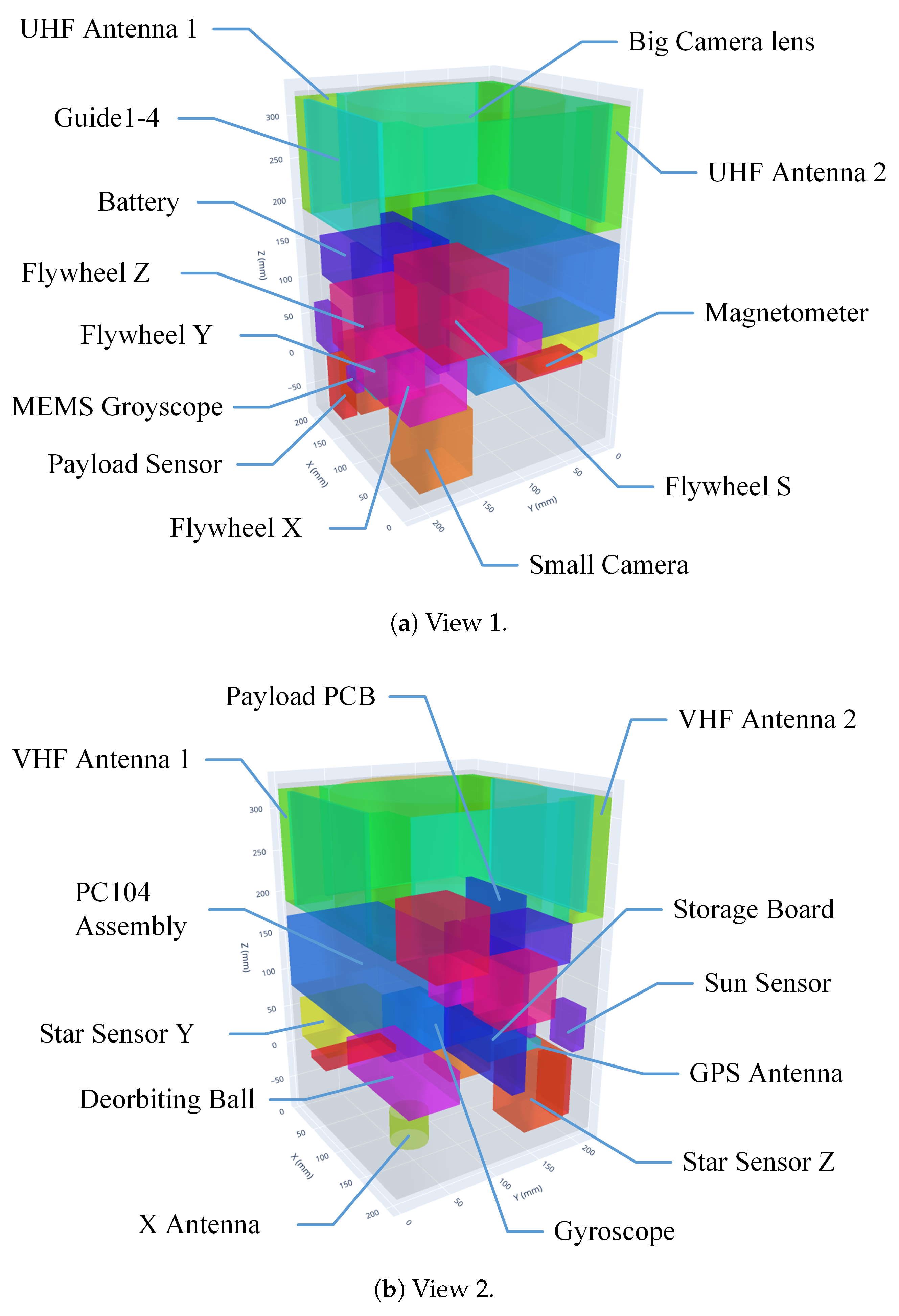
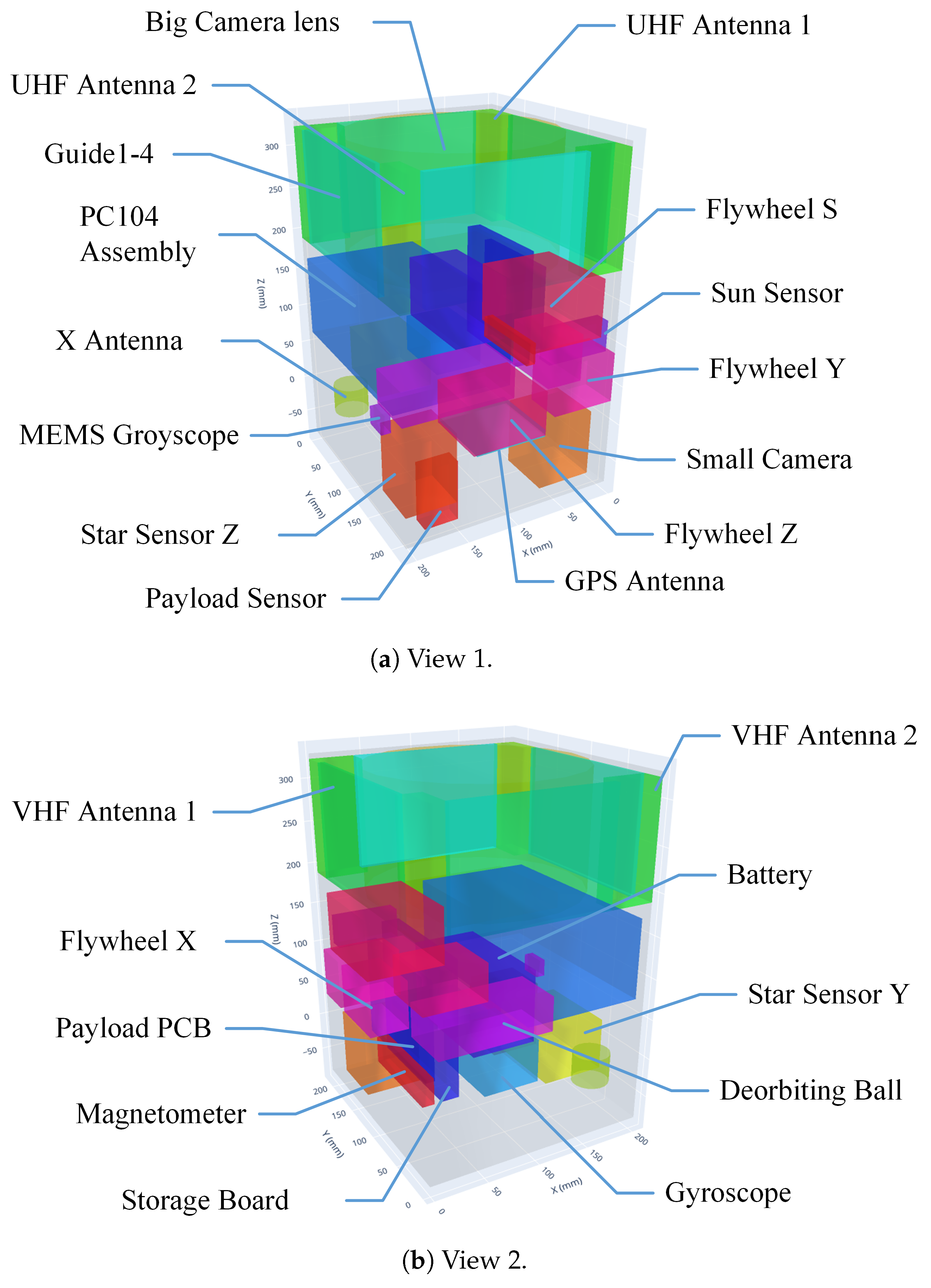
4. Engineering Case Study

To thoroughly demonstrate the effectiveness and practicality of the proposed GRASP and NSGA-III hybrid optimization framework, this section presents a detailed engineering case study of the ASRTU Friendship MicroSat, the first CubeSat jointly developed by Chinese and Russian university students. The case study demonstrates the application of the proposed method across three design stages, highlighting its adaptability to varying complexity and practical constraints. The external appearance of the ASRTU Friendship MicroSat is depicted in Figure 4.
The basic structural and envelope parameters of ASRTU Friendship MicroSat are shown in Table 1.

4.1. Initial Feasibility Analysis

At the start of the satellite design process, only component parameters and basic installation constraints were known, without any initial layout. Part of component dimensions were fixed in this stage. The primary goal was to generate multiple optimal layouts satisfying the interference constraints, serving as initial candidates for subsequent manual design refinements.
The basic parameters of components are shown in Table 2.
The GRASP parameters were configured as
GRASP iterations = 1 , RCL size = 10 , Initial population size = 1000 .
The NSGA-III parameters were set to
M U = 1000 , L A M B D A _ S I Z E = 2000 , G E N S = 100 , C X _ P R O B = 0 . 1 , M U T _ P R O B = 0 . 9 .
The scale factors were permitted to vary between 0.9 and 1.1, giving each size-adjustable component a 10% margin for dimensional tuning.
Applying the GRASP+NSGA-III method in the initial design stage efficiently generates multiple interference-free layouts aligned with preliminary objectives. This enlarges the search space and breaks the limits of manual design. Each optimization run took about 4500 s on an Intel i7-12600K CPU with 64 GB RAM. After removing duplicates, around 50 different and valid layouts were kept. In this calculation, the algorithm produced a Pareto front with 56 non-dominated solutions, as listed in Table 3. For clarity, only one representative layout (solution 3), which was later fine-tuned by the design team, is reported in Table 4 and shown in Figure 5.

4.2. Detailed Design Optimization

In this phase, the manually refined layout from the initial phase was used as the input, as is shown in Table 5. Design constraints were significantly tightened, with only a limited range of size variations permitted for several components, thus greatly increasing the difficulty of obtaining feasible layouts. The basic parameters of components are shown in Table 6.
The GRASP parameters were adjusted to
GRASP iterations = 5 , RCL size = 5 , Initial population size = 1000 .
Correspondingly, the NSGA-III parameters were adjusted to
M U = 1000 , L A M B D A _ S I Z E = 2000 , G E N S = 300 , C X _ P R O B = 0 . 1 , M U T _ P R O B = 0 . 9 .
The scale factors were permitted to vary between 0.9 and 1.1. By assigning the engineering objectives described in Section 2, the proposed algorithm returns layout configurations that can be applied directly in hardware integration. For the few components whose dimensions are still adjustable, the hybrid algorithm is able to obtain the largest feasible envelopes that do not violate any other objective or interference constraint, thus giving clear guidelines for the follow-on component design and the final satellite layout.
Each optimization run required approximately 6000 s on an i7-12600K processor (Intel, Santa Clara, CA, USA) with 64 GB RAM. In this study, the algorithm produced a Pareto front with four non-dominated solutions, as listed in Table 7. For clarity, only one representative layout (solution 2), which was chosen as the detailed layout solution, is reported in Table 8 and illustrated in Figure 6.

4.3. Final-Stage Adjustment and Trade-Off

During the final stage of design, a battery protection circuit board had to be integrated with the battery, which inevitably enlarged the battery’s envelope and forced a reassessment of its mounting surface. At this point, the overall satellite layout was almost frozen and very few components could still be moved or rescaled. Therefore, an additional optimization run was carried out to find engineering-feasible layouts that could accept the larger battery while still satisfying, as far as possible, the multiple design objectives defined earlier.
The initial layout for this phase is shown in Table 9. The basic parameters of components are shown in Table 10.
The GRASP parameters were set to
GRASP iterations = 10 , RCL size = 3 , Initial population size = 100 .
The NSGA-III parameters were set to
M U = 1000 , L A M B D A _ S I Z E = 2000 , G E N S = 100 , C X _ P R O B = 0 . 1 , M U T _ P R O B = 0 . 9 .
The scale factors were permitted to vary between 1 and 1.15. The optimization run required approximately 7300 s on an Intel i7-12600K processor with 64 GB RAM. In this study, the algorithm produced only one solution, as listed in Table 11. The solution is reported in Table 12 and illustrated in Figure 7. According to the calculation result, the width and height of battery component were able to be enlarged by 4% and 2% and give an extended space for the protection circuit board.

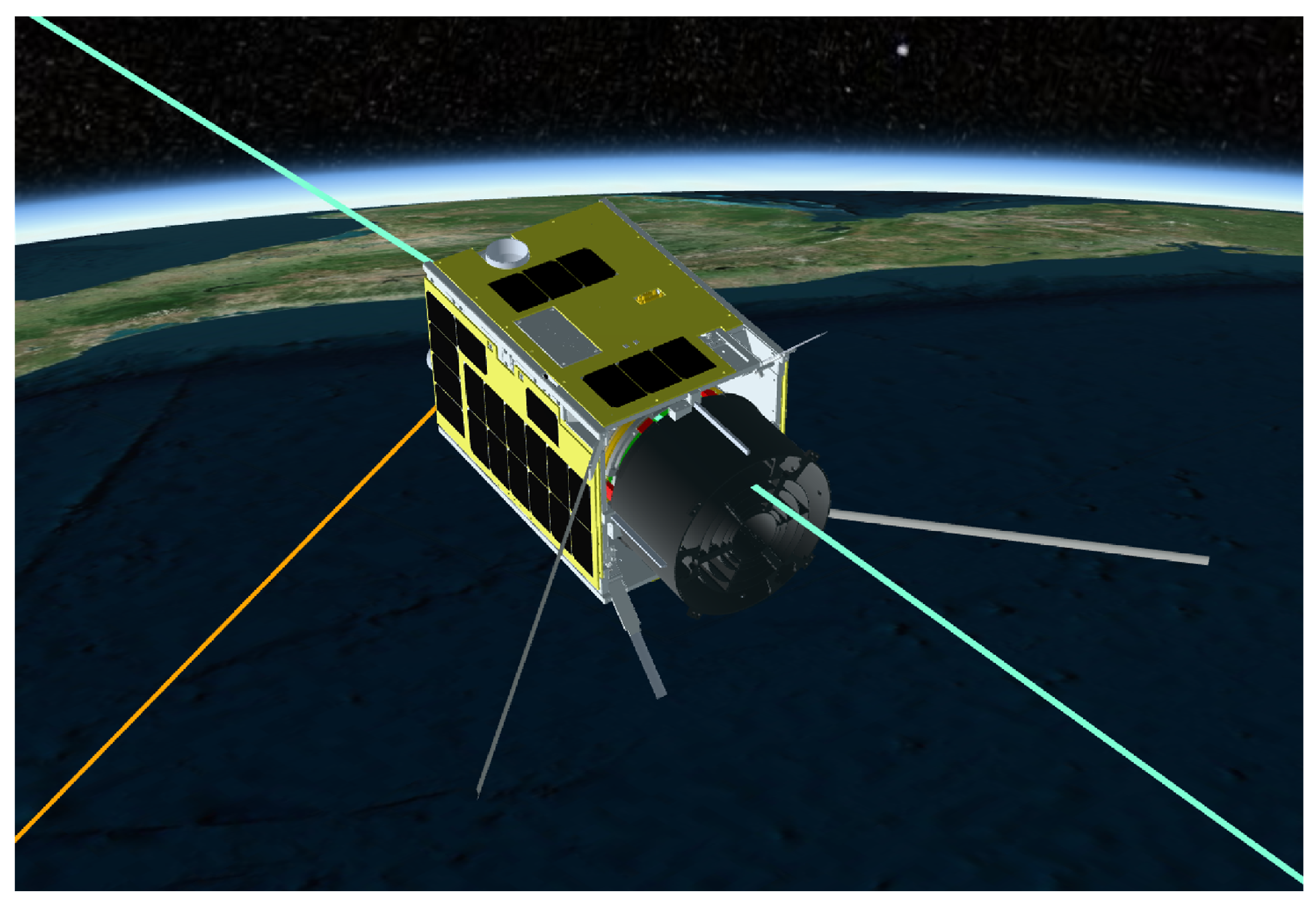
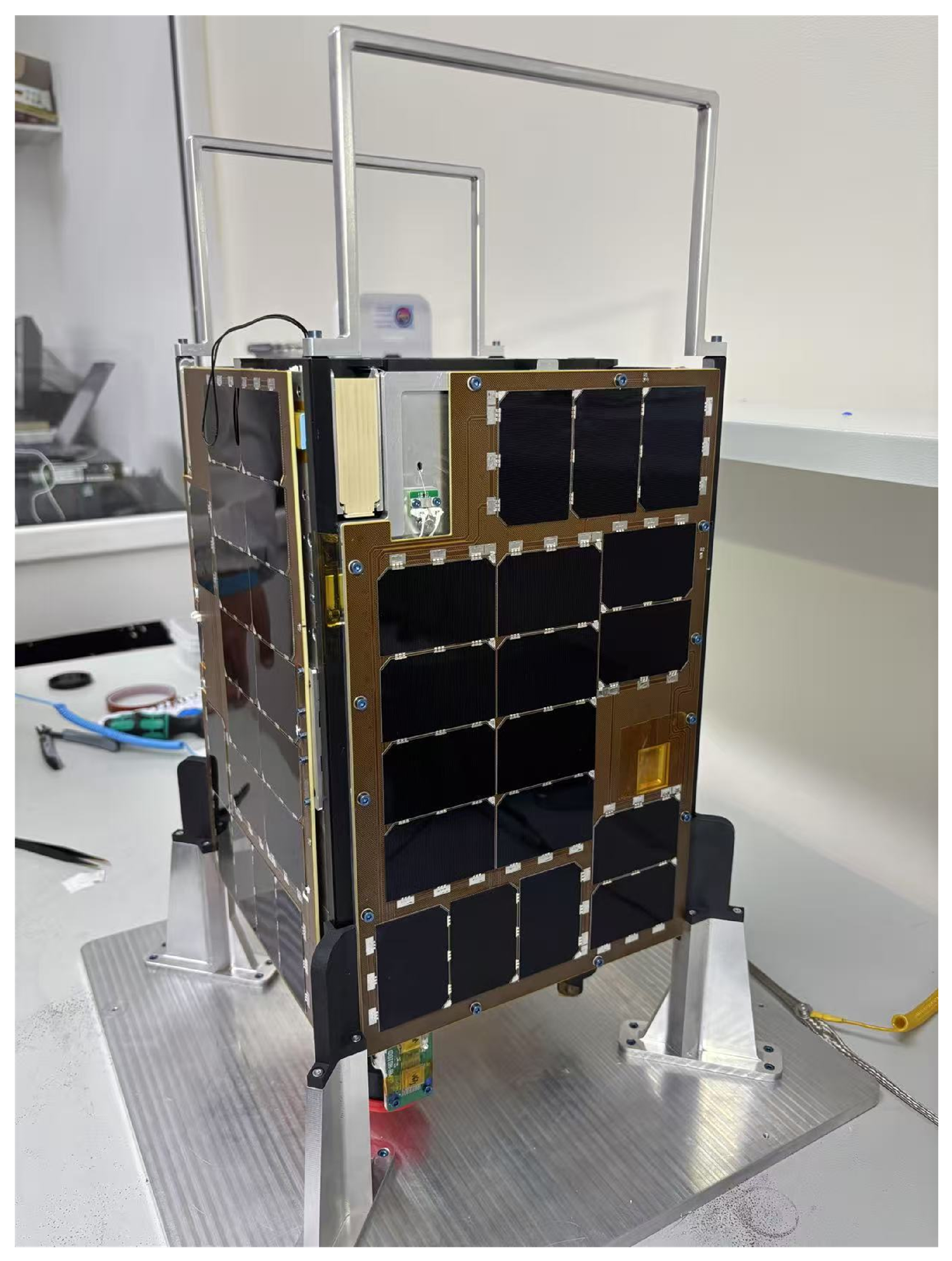
4.4. Ground Validation and In-Orbit Performance

The ASRTU Friendship MicroSat underwent comprehensive ground validation at the Research Center of Satellite Technology, Harbin Institute of Technology, in October 2023. Test results confirmed that the centroid deviation remained within 2 mm of the geometric center (Figure 8). The assembly result, shown in Figure 9, verified full compliance with all predefined layout constraints.
Following its launch on 5 Nov 2024, the satellite entered a stable orbit and began nominal operations. In-orbit thermal data from key subsystems, summarized in Table 13, indicated that temperatures remained within the specified operational range, confirming the effectiveness of the thermal design.

5. Conclusions

This paper has presented an engineering-oriented layout optimization and trade-off design methodology tailored to 12U CubeSats, based on a hybrid GRASP–NSGA-III framework. By combining GRASP’s efficient feasibility search with NSGA-III’s multi-objective diversity preservation, the proposed approach supports the rapid generation of interference-free candidate layouts, the balanced exploration of conflicting objectives, and fine-tuned refinement under tightened constraints. Custom crossover and mutation operators, along with a robust penalty scheme for interference, ensure that all returned designs are immediately implementable in real hardware integration.
The ASRTU Friendship MicroSat case study demonstrates the practical effectiveness of the method. The initial feasibility analysis efficiently produced numerous valid layouts, expanding the design possibilities beyond conventional manual approaches. Detailed and final-stage optimizations accommodated both strict size limits and the late addition of a battery protection board, while still achieving improvements in centroid offset, moment of inertia, and power distribution uniformity. Ground testing confirmed centroid deviations within ±2 mm, and in-orbit thermal measurements indicated that subsystem temperatures were maintained within specified operational limits, validating the effectiveness and practical relevance of the proposed optimization approach.
Compared with traditional packing- or DE-only methods, our hybrid GRASP–NSGA-III approach delivers faster convergence to feasible solutions, greater flexibility in iterative design workflows, and clear guidance on adjustable-component envelopes for follow-on engineering. Future work will explore integration of dynamic constraints (e.g., natural frequency) and extension to other CubeSat form factors, further broadening the applicability of this practical optimization framework.

Author Contributions

Conceptualization, J.Z. and C.Z.; methodology, J.Z.; software, J.Z.; validation, J.Z., Z.L. and L.L.; data curation, Z.L. and L.L.; writing, J.Z., Z.L. and L.L.; visualization, J.Z.; supervision, H.L.; project administration, H.L.; funding acquisition, H.L. All authors have read and agreed to the published version of the manuscript.

Funding

This research received no external funding.

Data Availability Statement

The data are available from the corresponding author upon reasonable request.

Conflicts of Interest

The authors declare no conflicts of interest.

Appendix A. Sensitivity Study of the Baseline-Bias Coefficient α

The coefficient α multiplies the Euclidean distance L L 0 2 between a candidate layout, L , and the baseline layout L 0 . A small α relaxes this penalty and encourages global exploration, whereas a large α keeps the optimization clustered around the baseline and accelerates convergence. Because the acceptable deviation is mission-dependent, α is left as a designer-tunable parameter.
To evaluate the influence of α , a sensitivity study was conducted with the Detailed Design Optimization task described in Section 4.2. Component properties and the baseline layout were kept identical to those in that demonstration. Three representative values were tested: α = 0 . 1 , 1, and 2. Each case was run under the same input parameters as those in the case in Section 4.2, yielding a Pareto front of non-dominated solutions.
Table A1, Table A2 and Table A3 list the solutions with the baseline distance d norm for each α . The single layout closest to the baseline for every run was extracted and is summarised in Table A4. The monotonic decrease in d norm confirms that increasing α forced the optimizer to stay nearer to the initial design, while a smaller value permitted wider exploration of the design space.
Table A1. Solutions for α = 0 . 1 (sorted by d norm ).
ID f 1 = V f 2 = C f 3 = I f 4 = T f 5 = D d norm
2−1.0164  × 10 7 0.5542.4186  × 10 5 3.562−3049.770.243
1−1.0176  × 10 7 0.6652.4266  × 10 5 3.562−3024.640.361
4−1.0110  × 10 7 0.6962.4208  × 10 5 3.724−3083.500.388
3−1.0125  × 10 7 1.0102.4388  × 10 5 3.724−3086.160.953
Table A2. Solutions for α = 1 (sorted by d norm ).
ID f 1 = V f 2 = C f 3 = I f 4 = T f 5 = D d norm
1−1.0176  × 10 7 0.5302.4175  × 10 5 3.562−3049.770.236
2−1.0164  × 10 7 0.6972.4283  × 10 5 3.724−3096.450.390
4−1.0368  × 10 7 0.7012.4206  × 10 5 3.562−3083.500.414
3−1.0122  × 10 7 0.8462.4298  × 10 5 3.562−3091.270.663
Table A3. Solutions for α = 2 (sorted by d norm ).
ID f 1 = V f 2 = C f 3 = I f 4 = T f 5 = D d norm
1−1.0176  × 10 7 0.5272.4173  × 10 5 4.766−3083.580.049
2−1.0162  × 10 7 0.6782.4276  × 10 5 3.724−3057.550.359
4−1.0122  × 10 7 0.7062.4206  × 10 5 3.562−3083.500.422
3−1.0137  × 10 7 0.7972.4289  × 10 5 3.562−3091.270.575
5−1.0101  × 10 7 0.9882.4391  × 10 5 3.724−3091.430.913
Table A4. Representative solution for each α (closest to baseline).
α ID f 1 = V f 2 = C f 3 = I f 4 = T f 5 = D d norm
0.12−1.0164  × 10 7 0.5542.4186  × 10 5 3.562−3049.770.243
11−1.0176  × 10 7 0.5302.4175  × 10 5 3.562−3049.770.236
21−1.0176  × 10 7 0.5272.4173  × 10 5 4.766−3083.580.049

References

  1. Heidt, H.; Puig-Suari, J.; Moore, A.; Nakasuka, S.; Twiggs, R. CubeSat: A new generation of picosatellite for education and industry low-cost space experimentation. In Proceedings of the the 14th Annual/USU Conference on Small Satellites, Logan, UT, USA, 21–24 August 2000. [Google Scholar]
  2. Chin, A.; Coelho, R.; Nugent, R.; Munakata, R.; Puig-Suari, J. CubeSat: The pico-satellite standard for research and education. In Proceedings of the AIAA SPACE 2008 Conference & Exposition, San Diego, CA, USA, 9–11 September 2008. [Google Scholar]
  3. Poghosyan, A.; Golkar, A. CubeSat evolution: Analyzing CubeSat capabilities for conducting science missions. Prog. Aerosp. Sci. 2017, 88, 59–83. [Google Scholar] [CrossRef]
  4. Macario-Rojas, A.; Smith, K. Spiral coning manoeuvre for in-orbit low thrust characterisation in CubeSats. Aerosp. Sci. Technol. 2017, 71, 337–346. [Google Scholar] [CrossRef]
  5. Imken, T.; Castillo-Rogez, J.; He, Y.; Baker, J.; Marinan, A. CubeSat flight system development for enabling deep space science. In Proceedings of the 2017 IEEE Aerospace Conference, Big Sky, MT, USA, 4–11 March 2017; IEEE: Piscataway, NJ, USA, 2017; pp. 1–14. [Google Scholar]
  6. Gardner, T.; Cheetham, B.; Forsman, A.; Meek, C.; Kayser, E.; Parker, J.; Thompson, M.; Latchu, T.; Rogers, R.; Bryant, B.; et al. Capstone: A Cubesat Pathfinder for the Lunar Gateway Ecosystem; Utah State University: Logan, UT, USA, 2021. [Google Scholar]
  7. Schoolcraft, J.; Klesh, A.; Werne, T. MarCO: Interplanetary mission development on a CubeSat scale. In Space Operations: Contributions from the Global Community; Springer: Cham, Switzerland, 2017; pp. 221–231. [Google Scholar]
  8. Peral, E.; Tanelli, S.; Statham, S.; Joshi, S.; Imken, T.; Price, D.; Sauder, J.; Chahat, N.; Williams, A. RainCube: The first ever radar measurements from a CubeSat in space. J. Appl. Remote Sens. 2019, 13, 032504. [Google Scholar] [CrossRef]
  9. Huggins, G.M.; Talaksi, A.; Andrews, D.; Lightsey, E.G.; Cavender, D.; McQueen, D.; Williams, H.; Diaz, C.; Baker, J.; Kowalkowski, M. Development of a CubeSat-scale green monopropellant propulsion system for NASA’s lunar flashlight mission. In Proceedings of the AIAA Scitech 2021 Forum, Virtual Event, 11–15 & 19–21 January 2021; p. 1976. [Google Scholar]
  10. Nason, I.; Puig-Suari, J.; Twiggs, R. Development of a family of picosatellite deployers based on the CubeSat standard. In Proceedings of the Proceedings, IEEE Aerospace Conference, Big Sky, MT, USA, 9–16 March 2002; IEEE: Piscataway, NJ, USA, 2002; Volume 1, p. 1. [Google Scholar]
  11. Young, J.; Inlow, S.; Bender, B. Solving thermal control challenges for CubeSats: Optimizing passive thermal design. In Proceedings of the 2019 IEEE Aerospace Conference, Big Sky, MT, USA, 2–9 March 2019; IEEE: Piscataway, NJ, USA, 2019; pp. 1–7. [Google Scholar]
  12. Li, J.; Post, M.; Wright, T.; Lee, R. Design of Attitude Control Systems for CubeSat-Class Nanosatellite. J. Control Sci. Eng. 2013, 2013, 657182. [Google Scholar] [CrossRef]
  13. Wang, Y.S.; Teng, H.F.; Shi, Y.J. Cooperative co-evolutionary scatter search for satellite module layout design. Eng. Comput. 2009, 26, 761–785. [Google Scholar] [CrossRef]
  14. Feng, E.; Wang, X.; Wang, X.; Teng, H. An algorithm of global optimization for solving layout problems. Eur. J. Oper. Res. 1999, 114, 430–436. [Google Scholar] [CrossRef]
  15. Che, C.; Teng, H.; Wang, Y. Constrained circles packing test problems: All the optimal solutions known. Int. J. Comput. Math. 2010, 87, 2887–2902. [Google Scholar] [CrossRef]
  16. Teng, H.f.; Chen, Y.; Zeng, W.; Shi, Y.j.; Hu, Q.h. A dual-system variable-grain cooperative coevolutionary algorithm: Satellite-module layout design. IEEE Trans. Evol. Comput. 2009, 14, 438–455. [Google Scholar] [CrossRef]
  17. Xiao, R.B.; Xu, Y.C.; Amos, M. Two hybrid compaction algorithms for the layout optimization problem. BioSystems 2007, 90, 560–567. [Google Scholar] [CrossRef]
  18. Xu, Z.Z.; Zhong, C.Q.; Teng, H.F. Assignment and layout integration optimization for simplified satellite re-entry module component layout. Proc. Inst. Mech. Eng. Part G J. Aerosp. Eng. 2019, 233, 4287–4301. [Google Scholar] [CrossRef]
  19. Huo, J.Z.; Teng, H.F.; Sun, W.; Chen, J. Human-computer co-operative co-evolutionary method and its application to a satellite module layout design problem. Aeronaut. J. 2010, 114, 209–223. [Google Scholar] [CrossRef]
  20. Chen, X.; Liu, S.; Sheng, T.; Zhao, Y.; Yao, W. The satellite layout optimization design approach for minimizing the residual magnetic flux density of micro-and nano-satellites. Acta Astronaut. 2019, 163, 299–306. [Google Scholar] [CrossRef]
  21. Li, Z.; Zeng, Y.; Wang, Y.; Wang, L.; Song, B. A hybrid multi-mechanism optimization approach for the payload packing design of a satellite module. Appl. Soft Comput. 2016, 45, 11–26. [Google Scholar] [CrossRef]
  22. Chen, X.; Yao, W.; Zhao, Y.; Chen, X.; Zheng, X. A practical satellite layout optimization design approach based on enhanced finite-circle method. Struct. Multidiscip. Optim. 2018, 58, 2635–2653. [Google Scholar] [CrossRef]
  23. Zhang, J.; Guo, J.; Liu, Y.; Wang, Z.; Feng, Y.; Li, H. Component assignment and layout optimization for multi-module microsatellite considering variable module size. Acta Astronaut. 2022, 198, 36–44. [Google Scholar] [CrossRef]
  24. Cuco, A.P.C.; de Sousa, F.L.; Silva Neto, A.J. A multi-objective methodology for spacecraft equipment layouts. Optim. Eng. 2015, 16, 165–181. [Google Scholar] [CrossRef]
  25. Xu, Z.Z.; Jiang, F.; Zhong, C.Q.; Gou, Y.J.; Teng, H.F. Multi-objective layout optimization for an orbital propellant depot. Struct. Multidiscip. Optim. 2020, 61, 207–223. [Google Scholar] [CrossRef]
  26. Yan’gang, L.; Zheng, Q. A decision support system for satellite layout integrating multi-objective optimization and multi-attribute decision making. J. Syst. Eng. Electron. 2019, 30, 535–544. [Google Scholar]
  27. Fakoor, M.; Ghoreishi, S.M.N.; Sabaghzadeh, H. Spacecraft component adaptive layout environment (SCALE): An efficient optimization tool. Adv. Space Res. 2016, 58, 1654–1670. [Google Scholar] [CrossRef]
  28. Zhang, Z.; Han, Q.; Li, Y.; Wang, Y.; Shi, Y. An evolutionary multiagent framework for multiobjective optimization. Math. Probl. Eng. 2020, 2020, 9147649. [Google Scholar] [CrossRef]
  29. Zheng, Q.; YanGang, L. Multiobjective methodology for satellite cabin layout optimization considering space debris impact risk. J. Spacecr. Rocket. 2018, 55, 232–235. [Google Scholar] [CrossRef]
  30. Feo, T.A.; Resende, M.G. Greedy randomized adaptive search procedures. J. Glob. Optim. 1995, 6, 109–133. [Google Scholar] [CrossRef]
  31. Emmerich, M.T.; Deutz, A.H. A tutorial on multiobjective optimization: Fundamentals and evolutionary methods. Natural computing. 2018, 17, 585–609. [Google Scholar] [CrossRef] [PubMed]
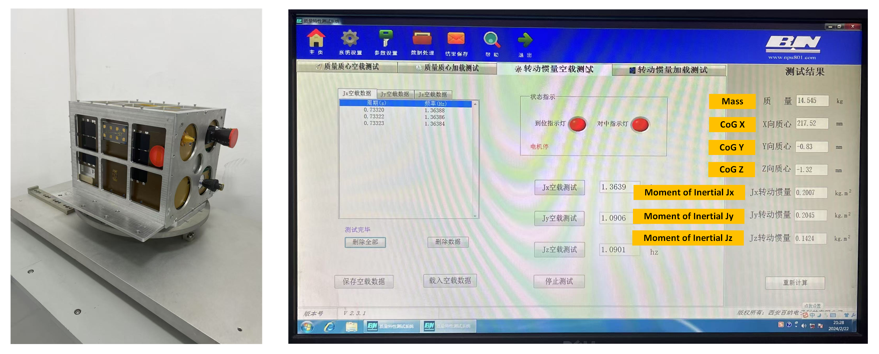
Figure 1. Simplified model of CubeSat module.
Aerospace 12 00506 g001
Figure 2. Simplified model of CubeSat components.
Aerospace 12 00506 g002
Figure 3. Detailed workflow of proposed hybrid GRASP-NSGA-III optimization framework.
Aerospace 12 00506 g003
Figure 4. External view of the ASRTU Friendship MicroSat.
Aerospace 12 00506 g004
Figure 5. Representative 3D layout (Initial Phase).
Aerospace 12 00506 g005
Figure 6. Representative 3D layout (detailed phase).
Aerospace 12 00506 g006
Figure 7. Representative 3D layout (final phase).
Aerospace 12 00506 g007
Figure 8. Ground test centroid deviation results.
Aerospace 12 00506 g008
Figure 9. MicroSat assembly process.
Aerospace 12 00506 g009
Table 1. Structural and envelope parameters.
ParameterValue
m sat 3.576 kg
c sat (103.78, 104.71, 148.07) mm
I s a t , x 158,857.62 kg·mm2
I s a t , y 157,233.84 kg·mm2
I s a t , z 114,844.09 kg·mm2
Envelope (X × Y × Z)206.3 × 216.3 × 328.5 mm
Extended volume length 80 . 0  mm
Table 2. Component basic parameters (initial phase).
NameShapeDimensions (mm)Mass (kg)Power (W)SurfacesAdjustable
Payload Sensorbox(32, 16, 75)0.020.1bottomnone
Star Sensor Zbox(50, 48, 89.8)0.11.276bottomnone
Small Camerabox(54, 54, 84.8)0.1221.5bottomnone
Big Camera cabinbox(104, 93, 17.7)10topnone
Big Camera lenscylinder(95, 95, 139)2.54topnone
Star Sensor Ybox(55, 60, 71.9)0.0111.276frontx, y, z, θ , l, w, h
X Antennacylinder(17, 17, 37.5)0.0340bottomnone
UHF Antenna-1box(40, 133, 21.5)0.0380rightnone
UHF Antenna-2box(40, 133, 21.5)0.0380leftnone
VHF Antenna-1box(40, 133, 21.5)0.0380backnone
VHF Antenna-2box(40, 133, 21.5)0.0380frontnone
Guide 1box(154, 133, 6)0.010leftnone
Guide 2box(144, 133, 6)0.010frontnone
Guide 3box(154, 133, 6)0.010rightnone
Guide 4box(144, 133, 6)0.010backnone
GPS Antennabox(69.4, 69.4, 9)0.0340bottomx, y, z, θ , l, w, h
Gyroscopebox(50, 50, 69)0.1852.5all surfacesx, y, z, θ , l, w, h
PC104 Assemblybox(183.4, 95.3, 100.3)1.74513front, back, left, rightx, y, z, θ , l, w, h
Payload PCBbox(102.7, 109.8, 8)0.0580.4all surfacesx, y, z, θ , l, w, h
Storage Boardbox(15.2, 152.8, 101.7)0.18810all surfacesx, y, z, θ , l, w, h
Batterybox(55, 74.2, 90)0.781all surfacesx, y, z, θ , l, w, h
Sun Sensorbox(59.3, 37, 15)0.0410backx, y, z, θ , l, w, h
MEMS Gyroscopebox(22.4, 22.4, 9)0.0070.187front, back, left, rightx, y, z, θ , l, w, h
Deorbiting Ballbox(120, 54.5, 43.6)0.50.055bottomx, y, z, θ , l, w, h
Flywheel Xbox(61, 61, 36.9)0.2370leftx, y, z, θ , l, w, h
Flywheel Ybox(61, 61, 36.9)0.2370.758backx, y, z, θ , l, w, h
Flywheel Zbox(72, 55, 65)0.2650.758backx, y, z, θ , l, w, h
Flywheel Sbox(86, 71.5, 73.1)0.2650.758leftx, y, z, θ , l, w, h
Magnetometerbox(85.1, 30.5, 10.5)0.010.451all surfacesx, y, z, θ , l, w, h
Table 3. Pareto front fitness (initial phase).
ID f 1 = V f 2 = C f 3 = I f 4 = T f 5 = D ID f 1 = V f 2 = C f 3 = I f 4 = T f 5 = D
1−9.7596  × 10 6 7.3042.3169  × 10 5 4.838−3195.2729−9.4153  × 10 6 8.8612.3078  × 10 5 5.090−3236.52
2−9.7223  × 10 6 5.0222.3770  × 10 5 4.846−2792.8230−9.4077  × 10 6 2.4362.5279  × 10 5 6.785−3480.76
3−9.6961  × 10 6 4.2482.4118  × 10 5 4.010−2680.2731−9.4031  × 10 6 7.2002.3160  × 10 5 4.282−2752.58
4−9.6944  × 10 6 8.3752.5496  × 10 5 4.281−3279.9432−9.3911  × 10 6 6.8242.3334  × 10 5 4.282−2747.88
5−9.6846  × 10 6 4.4602.3643  × 10 5 4.846−2786.6733−9.3819  × 10 6 4.0122.3914  × 10 5 4.846−2711.07
6−9.6715  × 10 6 4.3682.3618  × 10 5 4.846−2686.2434−9.3758  × 10 6 2.2812.5237  × 10 5 6.785−3491.69
7−9.6609  × 10 6 7.8232.3265  × 10 5 4.838−3200.2335−9.3744  × 10 6 12.8172.3114  × 10 5 6.618−3631.56
8−9.6527  × 10 6 4.8792.3865  × 10 5 4.846−2787.0736−9.3595  × 10 6 9.5772.3208  × 10 5 3.263−3272.56
9−9.6401  × 10 6 7.6862.5642  × 10 5 4.337−3313.4137−9.3447  × 10 6 8.7312.3296  × 10 5 5.090−3280.15
10−9.6307  × 10 6 5.4742.3464  × 10 5 4.846−2707.9838−9.3364  × 10 6 2.1832.5318  × 10 5 6.785−3502.03
11−9.6242  × 10 6 7.2102.5722  × 10 5 4.337−3325.4239−9.3336  × 10 6 6.3232.3144  × 10 5 4.846−2756.46
12−9.6167  × 10 6 3.9982.3721  × 10 5 4.846−2699.4240−9.3236  × 10 6 8.9632.3136  × 10 5 5.090−3264.61
13−9.6064  × 10 6 8.3742.3049  × 10 5 4.838−3180.0541−9.3192  × 10 6 5.7622.4300  × 10 5 4.256−2862.58
14−9.5853  × 10 6 8.1862.3082  × 10 5 4.838−3170.5842−9.3095  × 10 6 9.3602.3113  × 10 5 4.962−3232.08
15−9.5769  × 10 6 4.6872.3765  × 10 5 4.846−2791.7343−9.3015  × 10 6 6.7192.4117  × 10 5 4.236−2841.13
16−9.5683  × 10 6 2.0702.5148  × 10 5 6.785−3457.7844−9.2869  × 10 6 3.6892.4958  × 10 5 6.829−3552.82
17−9.5663  × 10 6 6.6992.3185  × 10 5 4.846−2759.2845−9.2843  × 10 6 6.3822.3237  × 10 5 4.282−2755.48
18−9.5443  × 10 6 7.3932.3048  × 10 5 7.160−2744.1046−9.2795  × 10 6 6.3952.4206  × 10 5 4.236−2993.20
19−9.5263  × 10 6 7.3922.2825  × 10 5 7.160−2750.3647−9.2644  × 10 6 9.4112.3186  × 10 5 3.263−3297.64
20−9.5164  × 10 6 1.7212.5042  × 10 5 6.785−3448.1548−9.2516  × 10 6 12.1552.3287  × 10 5 6.618−3642.95
21−9.5131  × 10 6 8.3082.3190  × 10 5 5.090−3219.1149−9.2389  × 10 6 8.9822.3577  × 10 5 4.250−3030.15
22−9.5021  × 10 6 7.1392.3092  × 10 5 4.282−2742.8450−9.2295  × 10 6 4.2762.4954  × 10 5 6.829−3479.01
23−9.4866  × 10 6 8.3432.5621  × 10 5 4.281−3287.5451−9.2275  × 10 6 6.1872.3228  × 10 5 4.282−2736.81
24−9.4774  × 10 6 3.9742.3806  × 10 5 4.846−2703.9552−9.2119  × 10 6 6.4932.3218  × 10 5 4.785−2799.13
25−9.4608  × 10 6 4.1442.3808  × 10 5 4.846−2714.5453−9.2020  × 10 6 9.6802.3044  × 10 5 5.090−3229.01
26−9.4406  × 10 6 6.6932.3239  × 10 5 4.846−2751.8154−9.1838  × 10 6 9.9662.3080  × 10 5 5.090−3242.81
27−9.4294  × 10 6 1.9062.5149  × 10 5 6.785−3469.5855−9.1666  × 10 6 6.5582.3117  × 10 5 4.282−2745.57
28−9.4268  × 10 6 6.3252.3016  × 10 5 4.282−2742.8256−9.1243  × 10 6 9.8872.3106  × 10 5 5.090−3237.34
Table 4. Representative solution (initial phase).
ComponentSurfacex (mm)y (mm)z (mm) θ (°)Scales
Payload Sensorbottom169.3201.3−33.50[1, 1, 1]
Star Sensor Zbottom170.3168.8−20.90[1, 1, 1]
Small Camerabottom36.5174.8−32.40[1, 1, 1]
Big Camera cabintop103.15106.09180.640[1, 1, 1]
Big Camera lenstop103.15108.15259.0[1, 1]
Star Sensor Yfront50.035.9546.1390[0.95, 1, 1]
X Antennabottom177.330.0−18.75[1, 1]
UHF Antenna 1right195.55196.3256.00[1, 1, 1]
UHF Antenna 2left10.7520.0256.00[1, 1, 1]
VHF Antenna 1back20.0205.55256.00[1, 1, 1]
VHF Antenna 2front186.310.75256.00[1, 1, 1]
Guide 1left3.0117.8256.00[1, 1, 1]
Guide 2front93.53.0256.00[1, 1, 1]
Guide 3right203.398.5256.00[1, 1, 1]
Guide 4back112.8213.3256.00[1, 1, 1]
GPS Antennabottom111.23172.974.9590[0.95, 0.9, 1.1]
Gyroscopebottom66.25102.5031.050[1.05, 0.9, 0.9]
PC104 Assemblyfront100.8550.14125.250[1.1, 0.95, 1]
Payload PCBback48.78212.70132.160[0.95, 0.95, 0.9]
Storage Boardright150.37127.2284.040[0.95, 1.1, 1.1]
Batteryback133.40175.80144.7590[0.9, 0.9, 0.9]
Sun Sensorback176.65208.8046.6990[0.9, 0.9, 1]
MEMS Gyroscopeback110.64212.2512.320[0.95, 1.1, 0.9]
Deorbiting Ballbottom137.0045.9120.730[0.95, 0.95, 0.95]
Flywheel Xleft18.45187.4548.9890[0.95, 0.9, 1]
Flywheel Yback68.98196.9348.980[0.95, 0.95, 1.05]
Flywheel Zback124.75183.8077.8090[1.05, 0.9, 1]
Flywheel Sleft40.21152.18125.1590[1.05, 0.9, 1.1]
Magnetometerbottom56.7838.304.9990[0.9, 1.1, 0.95]
Table 5. Initial layout (detailed phase).
NameFacex (mm)y (mm)z (mm) θ (deg)
Payload Sensorbottom169.30201.30−33.500
Star Sensor Zbottom170.30168.80−20.900
Small Camerabottom36.50174.80−32.400
Big Camera cabintop103.15106.09180.640
Big Camera lenstop103.15108.15259.00
Star Sensor Yfront136.8037.5732.000
X Antennabottom177.3030.00−18.75
UHF Antenna 1right195.55196.30297.550
UHF Antenna 2left10.7520.00297.550
VHF Antenna 1back20.00205.55297.550
VHF Antenna 2front186.3010.75297.550
GPS Antennabottom98.80172.654.500
Gyroscopefront75.5035.2034.500
PC104 Assemblyright151.15103.05117.600
Payload PCBleft5.0056.8595.900
Storage Boardfront19.8051.8594.900
Batteryfront65.0050.50102.830
Sun Sensorback40.15208.80115.000
MEMS Gyroscoperight201.80156.5548.800
Deorbiting Ballbottom109.15106.1527.000
Flywheel Xleft18.45142.6562.000
Flywheel Yback32.00197.8562.000
Flywheel Zback104.80183.8037.000
Flywheel Sleft36.55158.00135.250
Magnetometerleft5.2570.80169.800
Table 6. Component basic parameters (detailed phase).
NameShapeDimensions (mm)Mass (kg)Power (W)SurfacesAdjustable
Payload Sensorbox(32, 16, 75)0.020.1bottomnone
Star Sensor Zbox(50, 48, 89.8)0.11.276bottomnone
Small Camerabox(54, 54, 84.8)0.1221.50bottomnone
Big Camera cabinbox(104, 93, 17.7)10topnone
Big Camera lenscylinder(95, 95, 139)2.5004topnone
Star Sensor Ybox(55, 60, 71.9)0.0111.276frontx, y, z, θ , l, w, h
X Antennacylinder(17, 17, 37.5)0.0340bottomnone
UHF Antenna 1box(40, 133, 21.5)0.0380rightnone
UHF Antenna 2box(40, 133, 21.5)0.0380leftnone
VHF Antenna 1box(40, 133, 21.5)0.0380backnone
VHF Antenna 2box(40, 133, 21.5)0.0380frontnone
Guide 1box(154, 133, 6)0.010leftnone
Guide 2box(144, 133, 6)0.010frontnone
Guide 3box(154, 133, 6)0.010rightnone
Guide 4box(144, 133, 6)0.010backnone
GPS Antennabox(69.4, 69.4, 9)0.0340bottomx, y, z, θ , l, w, h
Gyroscopebox(50, 50, 69)0.1852.5all surfacesx, y, z, θ
PC104 Assemblybox(183.4, 95.3, 100.3)1.74513front, back, left, rightx, y, z, θ , l, w, h
Payload PCBbox(102.7, 109.8, 8)0.0580.4all surfacesx, y, z, θ , l, w, h
Storage Boardbox(15.2, 152.8, 101.7)0.18810all surfacesx, y, z, θ , l, w, h
Batterybox(55, 74.2, 90)0.7801all surfacesx, y, z, θ , l, w, h
Sun Sensorbox(59.3, 37, 15)0.0410backx, y, z, θ , l, w, h
MEMS Gyroscopebox(22.4, 22.4, 9)0.0070.187front, back, left, rightx, y, z, θ
Deorbiting Ballbox(120, 54.5, 43.6)0.50.055bottomx, y, z, θ , l, w, h
Flywheel Xbox(61, 61, 36.9)0.2370leftx, y, z, θ
Flywheel Ybox(61, 61, 36.9)0.2370.758backx, y, z, θ
Flywheel Zbox(72, 55, 65)0.2650.758backx, y, z, θ
Flywheel Sbox(86, 71.5, 73.1)0.2650.758leftx, y, z, θ
Magnetometerbox(85.1, 30.5, 10.5)0.0100.451all surfacesx, y, z, θ
Table 7. Pareto front fitness (detailed phase).
ID f 1 = V f 2 = C f 3 = I f 4 = T f 5 = D
1−1.0176  × 10 7 0.6652.4266  × 10 5 3.562−3024.64
2−1.0164  × 10 7 0.5542.4186  × 10 5 3.562−3049.77
3−1.0125  × 10 7 1.0102.4388  × 10 5 3.724−3086.16
4−1.0110  × 10 7 0.6962.4208  × 10 5 3.724−3083.50
Table 8. Representative solution (detailed phase).
ComponentSurfacex (mm)y (mm)z (mm) θ (deg)Scales
Payload Sensorbottom169.3201.3−33.50[1,1,1]
Star Sensor Zbottom170.3168.8−20.90[1, 1, 1]
Small Camerabottom36.5174.8−32.40[1, 1, 1]
Big Camera cabintop103.15106.09180.640[1, 1, 1]
Big Camera lenstop103.15108.15259[1, 1]
Star Sensor Yfront136.837.56632.00[1, 1, 1]
X Antennabottom177.330−18.75[1, 1]
UHF Antenna 1right195.55196.32560[1, 1, 1]
UHF Antenna 2left10.75202560[1, 1, 1]
VHF Antenna 1back20205.552560[1, 1, 1]
VHF Antenna 2front186.310.752560[1, 1, 1]
Guide 1left3117.82560[1, 1, 1]
Guide 2front93.532560[1, 1, 1]
Guide 3right203.398.52560[1, 1, 1]
Guide 4back112.8213.32560[1, 1, 1]
GPS Antennabottom98.8172.654.50[1, 1, 1]
Gyroscopefront7534.53590[1, 1, 1]
PC104 Assemblyright151.15103.52118.5890[1.02, 1.02, 1.2]
Payload PCBleft556.8595.90[1, 1, 1]
Storage Boardback19.851.8594.90[1, 1, 1]
Batteryfront67.549.5100.8250[1.1, 1.1, 1.1]
Sun Sensorback40.15208.81150[1, 1, 1]
MEMS Gyroscoperight201.8161.241.20[1, 1, 1]
Deorbiting Ballbottom110107.27323.5640[1, 1, 1.08]
Flywheel Xleft18.45140.560.590[1, 1, 1]
Flywheel Yback30.5197.8560.590[1, 1, 1]
Flywheel Zback106183.837.50[1, 1, 1]
Flywheel Sleft36.55153135.750[1, 1, 1]
Magnetometerleft5.2552.5525.250[1, 1, 1]
Table 9. Initial layout (final phase).
NameFacex (mm)y (mm)z (mm) θ (deg)
Payload Sensorbottom169.30201.30−33.500
Star Sensor Zbottom170.30168.80−20.900
Small Camerabottom36.50174.80−32.400
Big Camera cabinnone103.15106.09180.640
Big Camera lenstop103.15108.15259.00
Star Sensor Yfront136.8037.5732.000
X Antennabottom177.3030.00−18.75
UHF Antenna 1right195.55196.30297.550
UHF Antenna 2left10.7520.00297.550
VHF Antenna 1back20.00205.55297.550
VHF Antenna 2front186.3010.75297.550
GPS Antennabottom98.80172.654.500
Gyroscopefront75.5035.2034.500
PC104 Assemblyright151.15103.05117.600
Payload PCBleft5.0056.8595.900
Storage Boardfront19.8051.8594.900
Batteryfront65.0050.50102.830
Sun Sensorback40.15208.80115.000
MEMS Gyroscoperight201.80156.5548.800
Deorbiting Ballbottom109.15106.1527.000
Flywheel Xleft18.45142.6562.000
Flywheel Yback32.00197.8562.000
Flywheel Zback104.80183.8037.000
Flywheel Sleft36.55158.00135.250
Magnetometerleft5.2570.80169.800
Table 10. Component basic parameters (final phase).
NameShapeDimensions (mm)Mass (kg)Power (W)SurfacesAdjustable
Payload Sensorbox(32, 16, 75)0.020.10bottomnone
Star Sensor Zbox(50, 48, 89.8)0.101.276bottomnone
Small Camerabox(54, 54, 84.8)0.1221.50bottomnone
Big Camera cabinbox(104, 93, 17.7)1.000topnone
Big Camera lenscylinder(95, 95, 139)2.504topnone
Star Sensor Ybox(55, 60, 71.9)0.0111.276frontx, y, z, θ , l, w, h
X Antennacylinder(17, 17, 37.5)0.0340bottomnone
UHF Antenna 1box(40, 133, 21.5)0.0380rightnone
UHF Antenna 2box(40, 133, 21.5)0.0380leftnone
VHF Antenna 1box(40, 133, 21.5)0.0380backnone
VHF Antenna 2box(40, 133, 21.5)0.0380frontnone
Guide 1box(154, 133, 6)0.010leftnone
Guide 2box(144, 133, 6)0.010frontnone
Guide 3box(154, 133, 6)0.010rightnone
Guide 4box(144, 133, 6)0.010backnone
GPS Antennabox(69.4, 69.4, 9)0.0340bottomx, y, z, θ , l, w, h
Gyroscopebox(50, 50, 69)0.1852.5all surfacesx, y, z, θ
PC104 Assemblybox(201.7, 104.8, 110.3)1.74513front, back, left, rightx, y, z, θ , l, w, h
Payload PCBbox(102.7, 109.8, 8)0.0580.4all surfacesx, y, z, θ
Storage Boardbox(15.2, 152.8, 101.7)0.18810all surfacesx, y, z, θ
Batterybox(60.5, 81.65, 99)0.7801all surfacesx, y, z, θ , l, w, h
Sun Sensorbox(59.3, 37, 15)0.0410backnone
MEMS Gyroscopebox(22.4, 22.4, 9)0.0070.187front, back, left, rightx, y, z, θ
Deorbiting Ballbox(132, 60, 48)0.5000.055bottomnone
Flywheel Xbox(61, 61, 36.9)0.2370leftx, y, z, θ
Flywheel Ybox(61, 61, 36.9)0.2370.758backx, y, z, θ
Flywheel Zbox(72, 55, 65)0.2650.758backx, y, z, θ
Flywheel Sbox(86, 71.5, 73.1)0.2650.758leftx, y, z, θ
Magnetometerbox(85.1, 30.5, 10.5)0.0100.451all surfacesx, y, z, θ
Table 11. Pareto front fitness (final phase).
ID f 1 = V f 2 = C f 3 = I f 4 = T f 5 = D
1−1.0637  × 10 7 0.2782.4370  × 10 5 4.642−2946.12
Table 12. Representative solution (final phase).
ComponentSurfacex (mm)y (mm)z (mm) θ (deg)Scales
Payload Sensorbottom169.3201.3−33.50[1,1,1]
Star Sensor Zbottom170.3168.8−20.90[1, 1, 1]
Small Camerabottom36.5174.8−32.40[1, 1, 1]
Big Camera cabintop103.15106.09180.640[1, 1, 1]
Big Camera lenstop103.15108.15259[1, 1]
Star Sensor Yfront136.837.56632.00[1, 1, 1]
X Antennabottom177.330−18.75[1, 1]
UHF Antenna 1right195.55196.32560[1, 1, 1]
UHF Antenna 2left10.75202560[1, 1, 1]
VHF Antenna 1back20.0205.552560[1, 1, 1]
VHF Antenna 2front186.310.752560[1, 1, 1]
GPS Antennabottom98.8172.654.50[1, 1, 1]
Gyroscopefront75.034.535.00[1, 1, 1]
PC104 Assemblyright151.15100.85117.400[1, 1, 1]
Payload PCBleft4.056.3594.90[1, 1, 1]
Storage Boardfront17.650.8596.40[1, 1, 1]
Batteryfront65.2549.5102.4580[1, 1.04, 1.02]
Sun Sensorback40.15208.8115.00[1, 1, 1]
MEMS Gyroscoperight201.8156.251.20[1, 1, 1]
Deorbiting Ballbottom109.15106.1527.00[1, 1, 1]
Flywheel Xleft18.45140.560.50[1, 1, 1]
Flywheel Yback30.5197.8560.50[1, 1, 1]
Flywheel Zback106.0183.837.50[1, 1, 1]
Flywheel Sleft36.55158.0135.750[1, 1, 1]
Guide 1left3.0117.8256.00[1, 1, 1]
Guide 2front93.53.0256.00[1, 1, 1]
Guide 3right203.398.5256.00[1, 1, 1]
Guide 4back112.8213.3256.00[1, 1, 1]
Magnetometerback42.55211.05170.250[1, 1, 1]
Table 13. In-orbit thermal performance.
SubsystemMin. Temp (°C)Max. Temp (°C)Nominal Range (°C)
PC104 Assembly1428−10 to 45
Gyroscope615−15 to 45
Flywheel X1824−15 to 45
Flywheel Y917−15 to 45
Flywheel Z1725−15 to 45
Flywheel S1118−15 to 45
Big Camera cabin816−15 to 45
Battery9160 to 30
Disclaimer/Publisher’s Note: The statements, opinions and data contained in all publications are solely those of the individual author(s) and contributor(s) and not of MDPI and/or the editor(s). MDPI and/or the editor(s) disclaim responsibility for any injury to people or property resulting from any ideas, methods, instructions or products referred to in the content.

