Abstract
For the diverse payloads of Reusable Launch Vehicles and the inevitable problem of change in the center of mass, this paper proposes an incremental nonlinear dynamic inversion considering centroid variation control. Regarding the trans-atmosphere flight environment, the six-degree-of-freedom dynamics model considering centroid shift, Earth rotation, and the Clairaut Ellipsoid Model is established to improve model accuracy. An incremental nonlinear dynamic inversion considering a centroid variation controller with excellent dynamic performance and adjustment under the centroid variation is designed for the model, which fully meets the safety requirements of RLV reentry. An extended state observer considering centroid variation is proposed to solve the problem with difficult direct measurement of angular acceleration, which incorporates the influence of centroid variation into the known part to improve estimation accuracy and speed. Finally, the simulation results are provided to verify the robustness of the change of centroid position and good control quality with the proposed controller.
1. Introduction
A Reusable Launch Vehicle (RLV) is a type of hypersonic vehicle that can transport goods and personnel to the target orbit, reenter through the atmosphere after completing missions, and finally land on the ground [1]. In recent years, with the rise of the space economy, vertical takeoff and horizontal landing RLVs, such as the Dream Chaser, have attracted the attention of scholars and research institutions from various countries. This type of vehicle has advantages with low reuse costs, minimal overload, and high cargo ratio, which is one of the main directions of low-cost space cargo transportation technology [2].
Compared with traditional aircraft, a horizontal landing RLV has a wide variation range regarding the centroid and focus, which results in drastic changes in stability and places high demands on the centroid adaptability of control. For example, the maximum weight of the American RLV “Dream Chaser” [3,4] is about 14.5 tons, the payload is 5.5 tons, and the cargo ratio is around 38%. It means that the inertia and centroid are greatly affected by the payload, which brings uncertainties. RLV reentry velocity varies widely, which leads to a large range of focus changes; it also has serious nonlinear coupling and aerodynamic uncertainty problems [5]. In addition, RLVs needed to balance low-speed and high-speed performance during the designing, which results in poor stability and excessive sensitivity to changes in center of mass. In summary, compared with traditional aircraft, RLVs need to be more robust for centroid variation.
For centroid variation, engineers and scholars have proposed various solutions. The method of actively moving centroid control to adapt stability requirements is often used in the field of traditional engineering [6,7]. In one paper [8], the Airbus A380 aircraft (Airbus, Toulouse, France) adopts centroid control with moving fuel to adapt diverse payloads to keep the center of gravity within a reasonable range. In another paper [9], a gliding hypersonic warhead adjusts the centroid by a mass slider machine, which ensures stability during the entire flight. A horizontal landing RLV is a gliding hypersonic vehicle without fuel; installing a mass slider machine to RLVs can increase dead weight, which is not conducive for payload. For the above issues, centroid fault-tolerant control has become a better option. The method does not increase dead weight and has better adaptability for a lateral centroid shift, which can enhance the survivability of RLVs in damage.
Research on centroid fault-tolerant control can be divided into high-accuracy modeling and controller design. In terms of modeling, this paper [10] establishes a six-degree-of-freedom dynamics model to simulate centroid shift for damaged aircraft. The paper [11] establishes a six-degree-of-freedom model considering centroid variation under the airflow coordinate system to analyze the impact of change from the perspective of airflow angles. This paper [12] analyzes the effect of changes in inertia, lateral and longitudinal eccentric moments and other aspects based on a dynamics model considering centroid variation. However, the above models are all based on the assumption of the Earth plane. Due to the trans-atmosphere flight environment, the forces, moments, and motion variables of RLVs are more complex and non-ignorable. It is necessary to establish a more accurate model that considers Earth’s ellipsoid, rotation, latitude, longitude positions, and other factors [13] for RLVs.
For a centroid fault-tolerant controller design, this paper [14] proposes an adaptive control to address the problem of unknown inertia and an uncertain centroid, which estimates inertia using the Nussbaum function for unknown damaged aircraft. Different from the damage problem, the inertia of RLVs can be identified in space in advance [15,16], which can be used as an input parameter of the controller to enhance the reentry safety. This paper [17] designs a fault-tolerant controller based on a neural network called RBFNN. The simulations show good stability under centroid shift. Meanwhile, the neural network control is still in the early stages of development [18] and engineering applications are relatively less at present. This paper [19] designs a centroid fault-tolerant control based on multiple observers and the stability of the control is verified by simulations. The paper [20] proposes an integral sliding mode control to solve the problem of centroid variation. All the above methods ensure the robustness and stability but do not pay enough attention to control quality and dynamic performance. In engineering, in order to ensure flight safety, high robustness and good control quality are both important conditions.
For the above problems, this paper establishes a high-accuracy flight dynamics model that considers centroid shift, Earth rotation, and the Clairaut Ellipsoid Model for the trans-atmosphere flight environment. Based on the model, an incremental nonlinear dynamic inversion considering centroid variation control with both great robustness and control quality is proposed. The precise modeling makes full use of the centroid variation identified on orbit, which makes the method advantageous in terms of control surface anti-saturation. Traditional incremental nonlinear dynamic inversion control has been successfully used in X-35 and F-35 series aircraft [21,22,23], which shows potential in engineering applications of such a method. The innovative points of the paper are as follows:
- For the RLVs with a trans-atmosphere flight environment, a flight dynamic equation considering centroid shift, Earth rotation, and the Clairaut Ellipsoid Model is established, which improves model accuracy;
- Based on the high-precision model, an incremental nonlinear dynamic inversion considering centroid variation control is designed. The simulation results show that the controller performs well in dynamic performance, robustness, and control surface anti-saturation under centroid variation, which shows potential in engineering applications;
- To address the difficulty of directly measuring angular acceleration in engineering, an extended state observer considering centroid variation is used for the proposed controller, which incorporates the influence of centroid variation into the known part to improve estimation accuracy and speed.
2. Dynamics Model Considering Centroid Variation
This paper is based on the assumptions of a vehicle rigid body, Earth rotation, and the Clairaut Ellipsoid Model. This paper uses the Columbia space shuttle as a vehicle model, which is similar to horizontal landing RLVs [24].
2.1. Centroid Dynamics
As depicted in Figure 1, the centroid variation refers to the phenomenon that the centroid has moved relative to the origin point of the body coordinate frame. The definitions of other coordinate systems are shown in [25].
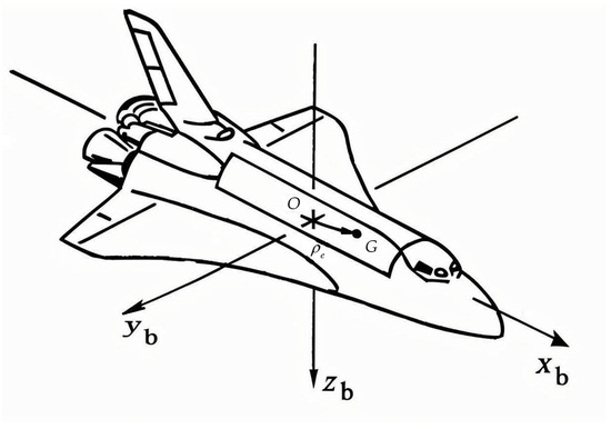
Figure 1.
View of centroid variation.
In the inertial coordinate system, the centroid position vector of the vehicle can be defined as follows:
where denotes the position vector of the origin point .
The relative speed of the vehicle in the Earth coordinate system can be written as:
where denotes the relative velocity vector of the origin point . represents the velocity vector of the centroid compared to the origin point . is the angular rate vector of the body coordinate system relative to the Earth coordinate system.
And the can be expressed as:
In the body coordinate system:
Considering the conditions of the Earth rotation and Clairaut Ellipsoid Model, the following centroid dynamic equation considering variation can be obtained by calculating the second-order derivative of Equation (1):
where is resultant force, represents mass, stands for the centroid position vector, and is the angular rate vector of the Earth.
And can be written as:
For , it can be expressed as:
Considering the rotation of the Earth, it yields:
Equation (6) can be written as:
where is the angular rate vector of the body coordinate system compared to the inertial frame coordinate.
Substituting Equations (3), (4) and (9) into (5), the centroid dynamic equation considering variation can be expressed as:
2.2. Rotational Dynamics
The original expression of angular momentum can be established as:
where represents the distance from the micro mass to the origin point . is the relative speed of the micro mass defined in the inertial frame coordinate system.
Expanding the above equation, one can obtain:
where denotes the distance from the micro mass to the centroid.
And it yields:
where represents the inertia matrix centered on the origin point .
After simplification, the expression for angular momentum can be obtained as:
By taking the derivative of Equation (11), the formula for the moment of momentum can be described as:
where:
where is three-axis moments.
The formula for the moment of momentum can be simplified as:
Substituting (14) into (17) and expanding it, the rotational dynamic equation considering centroid variation can be expressed as:
From Equations (10) and (18), the centroid dynamics and rotational dynamics will couple when the center of mass is changed, which makes the motion of the vehicle more complex. The influence of centroid variation on rotational dynamics is particularly significant [12].
2.3. Rotational Kinematics
To derive the incremental nonlinear dynamic inversion considering centroid variation control, the rotational kinematic equation is provided as follows. Because it is a relationship between velocity and position, the rotational kinematic equation is not affected by centroid variation. According to [26], the formula can be displayed as:
where , , and represent the angles of attack, sideslip, and bank. denotes the transformation matrix from the flight path coordinate system to the body coordinate system. and are the angles of track deviation and track inclination.
The relationship between and is expressed as:
where is the angle rate vector of the ground frame coordinate relative to the Earth frame coordinate.
2.4. Force and Moment Model
According to the parameters in reference [24], the aerodynamic force model can be written as follows:
where represents aerodynamic force. is the transformation matrix from the velocity coordinate system to the body coordinate system. is atmospheric density. denotes the reference area. stand for the basic aerodynamic coefficient. are incremental coefficients brought by elevators, ailerons, rudders, body flaps, and sideslip angles. , and denote ailerons, elevators, and rudders.
The moment model can be described as:
where denotes the wingspan. is the mean aerodynamic chord. represents the basic coefficient. stand for incremental coefficients brought by elevators, ailerons, rudders, body flaps, sideslip angles, and angle rates. , , and are the angle rates of the body coordinate system relative to the ground coordinate system.
Take the gravity into account and, simply, the resultant force of the RLV can be delivered as:
where represents the transformation matrix from the ground frame coordinate to the body coordinate system. is gravitational acceleration, whose calculation method can refer to [27].
Similarly, the three-axis moments can be simplified as:
Equations (23) and (24) are subsequently used for controller design.
2.5. Mass and Inertia Model
This paper simulates the changes of mass parameters by scaling the mass and inertia of the vehicle proportionally and moving the centroid. The weight coefficient of the entire vehicle is . The expression of mass can be written as:
where stands for the initial mass.
The inertia of the vehicle can be defined as:
where , and denote the area moment of inertia. , and represent the product of inertia. The centroid displacement is .
Based on the parallel axis and perpendicular axis theorem of inertia, each component can be described as:
where , and are the original area moment of inertia. is the original product of inertia.
In addition, the inertia matrix centered on the origin point : can be written as:
3. Incremental Nonlinear Dynamic Inversion Considering Centroid Variation Control
According to the theory of singular perturbation, state variables can be divided into fast variables (angle rates) and slow variables (angles), which can be separately designed as inner and outer controllers. Inner loop control with uncertain aerodynamic coefficients uses an incremental nonlinear dynamic inversion considering centroid variation control to improve robustness. Outer loop control designs a dynamic inversion control to ensure accuracy. The control structure is described in Figure 2.
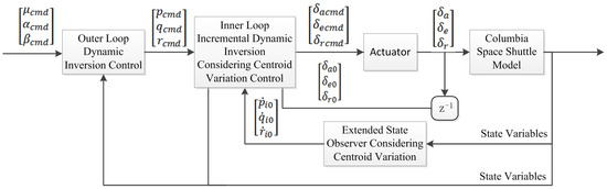
Figure 2.
Control structure.
3.1. Inner Loop Incremental Dynamic Inversion Control
To simplify Equations (23) and (24), the equations of three-axis force and moment can be formulated as follows:
where is dynamic pressure. are aerodynamic coefficients.
Substituting Equation (29) into (10), the centroid dynamic equation can be expressed as follows:
Substituting Equation (30) into (18), the rotational dynamics can be written as:
Substituting Equation (31) into (32), simplifying and writing the equation into an affine nonlinear form, one can obtain:
where represents the state variables . is the control surface state. and are as follows:
When the time interval is small enough, the rotational dynamics of the aircraft are mainly affected by the control surface deflection and the influence of state variables is relatively small, which can be ignored. So by the first-order Taylor expansion for Equation (33) at the state point and ignoring higher-order terms, it yields:
The partial derivative of the part can be ignored if the sampling frequency of the controller is sufficiently fast and one can obtain:
where are the angle rates at the state point . stands for the deflection of control surfaces at the state point .
The controller command can be designed as follows:
where represents the angle rate commands. The physical meaning of is the angle rates at the previous moment.
The method transforms the dependence on an accurate model into a sensing element. According to Equation (37), the controller can be expressed as:
The angular acceleration command is described as:
To sum up, inner loop incremental nonlinear dynamic inversion considering the centroid variation controller has been completed. The method takes the centroid variation into account, so that the control quality can be designed as expected under any centroid shift.
3.2. Outer Loop Dynamic Inversion Control
According to Equation (40), the inner loop controller requires the angle rates as commands, which means can be defined as a virtual control surface for incremental nonlinear dynamic inversion considering centroid variation control. From Equations (19) and (20), the outer loop dynamic inversion controller can be written as:
where is the input command of the dynamic inversion control, which can be expressed as:
Outer loop dynamic inversion control has been completed.
3.3. Extended State Observer Considering Centroid Variation
Regarding the problem of the difficulty of measuring angular acceleration directly, an extended state observer [28] considering centroid variation is proposed, which incorporates the influence of centroid variation into the known part to improves estimation accuracy and speed.
The extended state observer considers centroid variation based on a standard affine nonlinear equation. Based on Equation (33), regarding along with other disturbances as the total disturbance, the affine nonlinear equation can be written as:
where represents total disturbance.
The can be expressed as:
Based on Equation (43), the observer can be delivered as:
where denotes the estimated value of angular acceleration. is the estimated value of the angle rates. represents the estimated value of total disturbance. and are state observer coefficients.
To prove the convergence of the observer, subtracting Equation (45) from (43) and , one can obtain:
where denotes the estimated error of angle rates. is the estimated error of total disturbance.
When the is a bounded function, the convergence of the observer depends solely on the gain coefficients and . According to the bandwidth method of the extended state observer, the coefficients of the extended state observer can be designed as:
where is bandwidth.
Based on the method, the convergence of the extended state observer considering centroid variation can be guaranteed.
4. Simulation
In response, to verify the effectiveness of the incremental nonlinear dynamic inversion considering centroid variation control (INDICCV), two cases are designed based on the Columbia space shuttle [24]. Case 1 compares the control effect under the condition of normal state and centroid variation with aerodynamic coefficient uncertainties to demonstrate the robustness of the INDICCV. Case 2 compares the INDICCV, traditional nonlinear dynamic inversion control (NDI), and adaptive backstepping control (ABKS) [29] under the condition of centroid variation, which shows robustness, control quality, and control surface anti-saturation advantages of the proposed method.
The actuator is simulated by the second-order link, whose bandwidth is 5 Hz. The initial conditions are derived from the curve maneuvering trim [30]. The bandwidth of the extended state observer considering centroid variation is 20 rad/s. According to [24], the control surface’s deflection and its rate limit are shown in Table 1.

Table 1.
Control surface deflection limit.
4.1. Case 1. Control Performance Analysis
Case 1 compares the control effect under the condition of normal state and centroid variation with aerodynamic coefficient uncertainties. In view of the situation that the aerodynamic coefficient cannot be estimated accurately, a part of the parameters is offset to simulate uncertainties. The control gains are shown in Table 2. Initial conditions, centroid variation, and aerodynamic coefficient uncertainties are shown in Table 3.
Table 2.
Control gain of case 1.
Table 3.
Initial conditions of case 1.
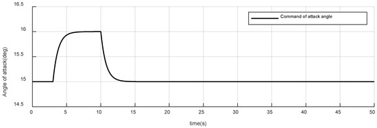
Figure 3.
Command of attack angle of case 1.
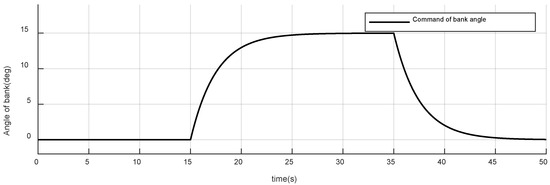
Figure 4.
Command of bank angle of case 1.
The initial command of the attack angle is 15 deg, which gradually rises to 16 deg at and progressively drops back to the initial value at ;
The initial command of the bank angle is 0 deg, which gradually rises to 15 deg at and progressively drops back to the initial value at .
The sideslip angle command remains at zero.
Figure 5, Figure 6 and Figure 7 are attitude responses. The black curve is the control command. Green, blue, and red curves are the normal state, centroid variation with +20% aerodynamic coefficient uncertainties, and centroid variation with −20% aerodynamic coefficient uncertainties, respectively. It is obvious that the INDICCV tracks commands well under the three conditions of normal state and centroid variation with uncertainties.
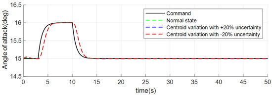
Figure 5.
Responses of attack angle of case 1.
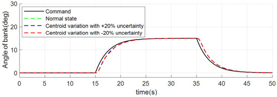
Figure 6.
Responses of bank angle of case 1.
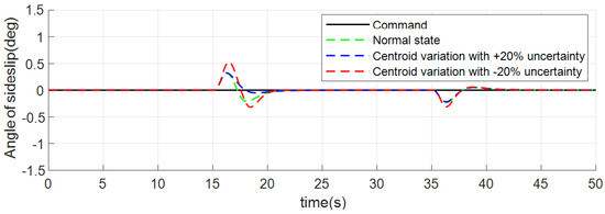
Figure 7.
Responses of sideslip angle of case 1.
Figure 8, Figure 9 and Figure 10 show the tracking error curve where the tracking error refers to the control command minus the actual attitude angle value. It can be observed that under three conditions, the maximum deviations for angle of attack tracking are 0.41 deg, those for bank tracking are 2.53 deg, and those for sideslip tracking are 0.31 deg, 0.32 deg, and 0.51 deg separately, which is relatively small and shows good performance.
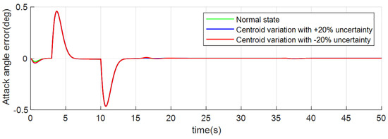
Figure 8.
Attack angle tracking error of case 1.
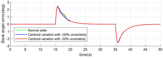
Figure 9.
Bank angle tracking error of case 1.
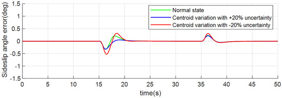
Figure 10.
Sideslip angle tracking error of case 1.
Figure 11, Figure 12 and Figure 13 depict angle rates. All the above figures (Figure 5, Figure 6, Figure 7, Figure 8, Figure 9, Figure 10, Figure 11, Figure 12 and Figure 13) show that the dynamic processes are almost stable under three conditions, which verifies the robustness and good control quality of the INDICCV.
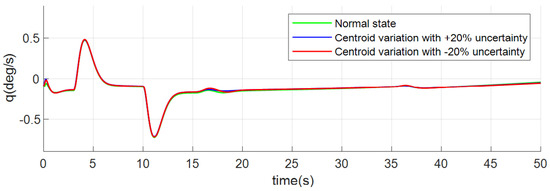
Figure 11.
Responses of pitch rate of case 1.
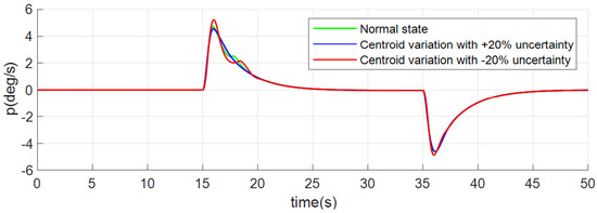
Figure 12.
Responses of roll rate of case 1.
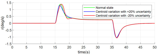
Figure 13.
Responses of yaw rate of case 1.
The control surface deflection curves are shown in Figure 14, Figure 15 and Figure 16. Although the angle and angle rate curves under the three conditions are similar, the control surface deflection will be different due to the centroid variation and aerodynamic coefficient uncertainties. It can be seen from Figure 15 and Figure 16 that when tracking the pitch angle command (), the deflection of the aileron and rudder in the normal state is stable at 0 deg. Meanwhile, under the two conditions of centroid variation with uncertainties, the ailerons are stabilized at 1.3 deg and 2 deg, respectively, and the rudders are stabilized at −6.1 deg and −8.9 deg, respectively, due to lateral and heading centroid shifts.
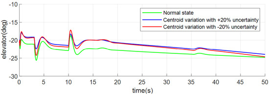
Figure 14.
Responses of elevator of case 1.
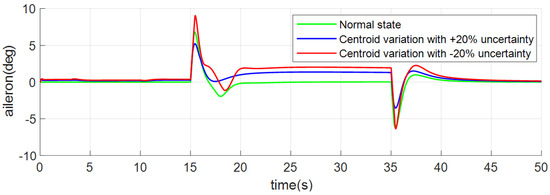
Figure 15.
Responses of aileron of case 1.
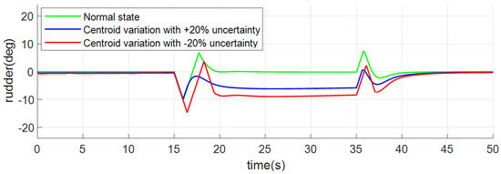
Figure 16.
Responses of rudder of case 1.
In summary, it can be observed that under variation and uncertainties, the INDICCV still maintains good dynamic performance and shows good robustness.
4.2. Case 2. Comparative Analysis
Case 2 compares the INDICCV, traditional dynamic inversion control, and adaptive backstepping control (ABKS) under the condition of centroid variation. The control gains are shown in Table 4. Initial conditions and centroid variation are shown in Table 5.
Table 4.
Control gain of case 2.
Table 5.
Initial conditions of case 2.
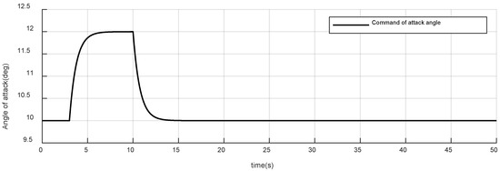
Figure 17.
Command of attack angle of case 2.
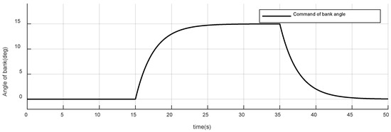
Figure 18.
Command of bank angle of case 2.
The initial command of the attack angle is 10 deg, which gradually rises to 12 deg at and progressively drops back to the initial value at ;
The initial command of the bank angle is 0 deg, which gradually rises to 15 deg at and progressively drops back to the initial value at ;
The sideslip angle command remains at zero.
Figure 19, Figure 20, Figure 21, Figure 22, Figure 23 and Figure 24 show the attitude response and tracking error curve. The black curve is the control command. The green, blue, and red curves are the INDICCV, NDI, and ABKS control, respectively. The INDICCV tracks commands well while the tracking of the NDI is poor under the influence of centroid variation due to the lack of robustness. The ABKS oscillates in responding to instructions. From Figure 25, Figure 26 and Figure 27, the oscillation is caused by the saturation of the control surface deflection rate.
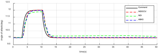
Figure 19.
Responses of attack angle of case 2.
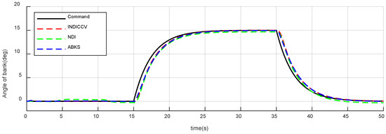
Figure 20.
Responses of bank angle of case 2.
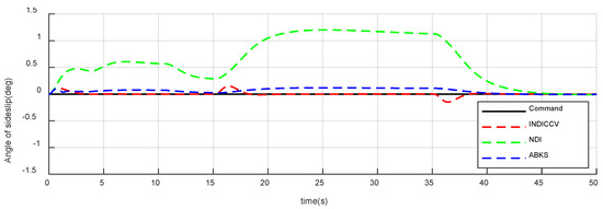
Figure 21.
Responses of sideslip angle of case 2.
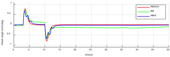
Figure 22.
Attack angle tracking error of case 2.
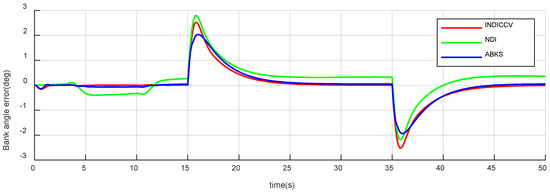
Figure 23.
Bank angle tracking error of case 2.
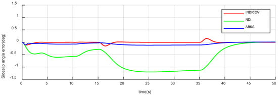
Figure 24.
Sideslip angle tracking error of case 2.
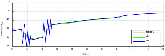
Figure 25.
Responses of elevator of case 2.
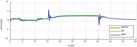
Figure 26.
Responses of aileron of case 2.
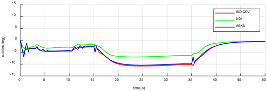
Figure 27.
Responses of rudder of case 2.
From Figure 22, Figure 23 and Figure 24, after the attack angle command of three controllers drops back to the initial value (), the steady-state errors are 0 deg, 0.14 deg, and 0.02 deg, respectively. After the bank angle command rises to 15 deg (), the steady-state errors are 0 deg, 0.32 deg, and 0.04 deg, separately; the sideslip angle steady-state errors are 0 deg, 1.2 deg, and 0.12 deg, respectively. In terms of steady-state error performance, the INDICCV is better than the comparison controllers.
Figure 25, Figure 26 and Figure 27 depict control surface deflection curves; The angle rates are shown in Figure 28, Figure 29 and Figure 30. It is obvious that the curves of the INDICCV are smooth, which is beneficial for engineering applications, while the comparison method of the ABKS experiences obvious oscillation, which is not conducive to engineering. From Figure 25, Figure 26 and Figure 27, it can be observed that the control surface deflection rate is saturated, which causes oscillation. The reason for saturation is that the ABKS not only adapts to external disturbance but also causes the instability of dynamic performance and unexpected overshoot, which brings a burden beyond the capacity of the actuator. The INDICCV shows better anti-saturation ability than the ABKS.
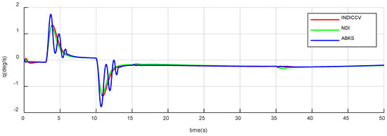
Figure 28.
Responses of pitch rate of case 2.
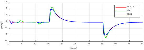
Figure 29.
Responses of roll rate of case 2.
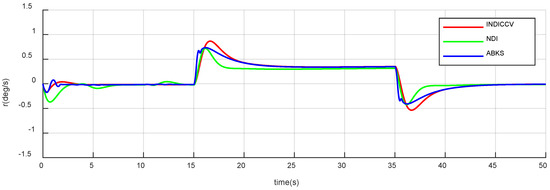
Figure 30.
Responses of yaw rate of case 2.
The INDICCV makes an attitude response to a standard second-order system response through dynamic inversion. The method takes centroid variation and inertia into account, which makes the dynamic performance still able to be designed as expected under centroid shift. The design considers both the robustness and control quality and ensures the safety of reentry.
In summary, the NDI has poor robustness and is unable to track control commands with high accuracy. The dynamic performance of the ABKS cannot be designed and is unstable and the unexpected overshoot causes the control surface deflection rate to be saturated. The INDICCV has no steady-state error, is better than the NDI in terms of tracking commands, and is superior to the ABKS in terms of anti-saturation ability. Both robustness and dynamic performance show advantages of the comparison method.
5. Conclusions
For the problem of the centroid variation of RLVs, this paper proposes an incremental nonlinear dynamic inversion considering centroid variation control. The conclusions are as follows:
- A flight dynamic equation considering centroid shift, Earth rotation, and the Clairaut Ellipsoid Model was established, which improved model accuracy;
- An incremental nonlinear dynamic inversion considering centroid variation control was designed for the problem of centroid variation and an extended state observer was introduced to solve the difficulty with measuring angular acceleration;
- Two sets of simulations were designed. Case 1 verified the robustness and excellent dynamic performance of the INDICCV under conditions of centroid variation with uncertainties. Case 2 compared the INDICCV with the NDI and ABKS, demonstrating the advantages of the INDICCV in steady-state error, anti-saturation ability, and robustness.
Author Contributions
Conceptualization, Q.T., J.G. and Y.F.; Methodology, Q.T.; Software, Q.T.; Validation, Q.T. and J.G.; Formal analysis, Q.T.; Investigation, Q.T.; Resources, Y.F.; Data curation, Q.T.; Writing—original draft, Q.T.; Writing—review & editing, J.G.; Visualization, Q.T.; Supervision, Y.F.; Project administration, Y.F. All authors have read and agreed to the published version of the manuscript.
Funding
This research received no external funding.
Data Availability Statement
The data presented in this study are available in the article.
Acknowledgments
The author sincerely thanks the editor and all anonymous reviewers for their comments, which helped to improve the quality of this article.
Conflicts of Interest
The authors declare no conflicts of interest.
Abbreviations
The following abbreviations are used in this manuscript:
| RLV | Reusable Launch Vehicle |
| INDICCV | Incremental Nonlinear Dynamic Inversion Considering Centroid Variation Control |
| NDI | Nonlinear Dynamic Inversion Control |
| ABKS | Adaptive Backstepping Control |
References
- Dietlein, I.; Bussler, L.; Stappert, S.; Wilken, J.; Sippel, M. Overview of system study on recovery methods for reusable first stages of future European launchers. CEAS Space J. 2024, 17, 71–88. [Google Scholar] [CrossRef]
- Baiocco, P. Overview of reusable space systems with a look to technology aspects. Acta Astronaut. 2021, 189, 10–25. [Google Scholar] [CrossRef]
- Ferretti, S. The Dream Chaser Spacecraft: Changing the Way the World Goes to Space. In Space Capacity Building in the XXI Century; Ferretti, S., Ed.; Springer International Publishing: Cham, Switzerland, 2020; pp. 123–137. [Google Scholar]
- Seedhouse, E. The Space Taxi Race. In SpaceX: Starship to Mars—The First 20 Years; Springer International Publishing: Cham, Switzerland, 2022; pp. 110–142. [Google Scholar]
- Kim, C.; Gwan, D.; Nam, M.S. Beyond the Atmosphere: The Revolution in Hypersonic Flight. Fusion Multidiscip. Res. Int. J. 2021, 2, 152–163. [Google Scholar]
- Li, J.; Gao, C.; Li, C.; Jing, W. A survey on moving mass control technology. Aerosp. Sci. Technol. 2018, 82, 594–606. [Google Scholar] [CrossRef]
- Isgandarov, I.A. Analytical and Simulation Model of a System for Non-Contact Determination of Aircraft Mass and Centre of Gravity. Meas. Tech. 2022, 64, 991–998. [Google Scholar] [CrossRef]
- Vogel, G. Flying the Airbus A380; Crowood: New York, NY, USA, 2012. [Google Scholar]
- Rogers, J.; Costello, M. A variable stability projectile using an internal moving mass. Proc. Inst. Mech. Eng. Part G J. Aerosp. Eng. 2009, 223, 927–938. [Google Scholar] [CrossRef]
- Asadi, D.; Ahmadi, K. Nonlinear robust adaptive control of an airplane with structural damage. Proc. Inst. Mech. Eng. Part G J. Aerosp. Eng. 2020, 234, 2076–2088. [Google Scholar] [CrossRef]
- Meng, Y.; Jiang, B.; Qi, R. Adaptive non-singular fault-tolerant control for hypersonic vehicle with unexpected centroid shift. IET Control. Theory Appl. 2019, 13, 1773–1785. [Google Scholar] [CrossRef]
- Ye, H.; Meng, Y. Adaptive Fault-Tolerant Control of Hypersonic Vehicles with Unknown Model Inertia Matrix and System Induced by Centroid Shift. Appl. Sci. 2023, 13, 830. [Google Scholar] [CrossRef]
- Yibo, D.; Xiaokui, Y.; Guangshan, C.; Jiashun, S. Review of control and guidance technology on hypersonic vehicle. Chin. J. Aeronaut. 2022, 35, 1–18. [Google Scholar]
- Wang, L.; Meng, Y.; Hu, S.; Peng, Z.; Shi, W. Adaptive fault-tolerant attitude tracking control for hypersonic vehicle with unknown inertial matrix and states constraints. IET Control. Theory Appl. 2023, 17, 1397–1412. [Google Scholar] [CrossRef]
- Duan, G.; Liu, G.P.; Pang, Z.H. Identification of Unknown Inertia Parameters of Spacecraft and Spacecraft Hovering. In Proceedings of the 2021 40th Chinese Control Conference (CCC), Shanghai, China, 26–28 July 2021; pp. 7595–7598. [Google Scholar]
- Morelli, E.A. Determining aircraft moments of inertia from flight test data. J. Guid. Control. Dyn. 2022, 45, 4–14. [Google Scholar] [CrossRef]
- Meng, Y.; Jiang, B.; Qi, R. Adaptive fault-tolerant attitude tracking control of hypersonic vehicle subject to unexpected centroid-shift and state constraints. Aerosp. Sci. Technol. 2019, 95, 105515. [Google Scholar] [CrossRef]
- Chai, R.; Tsourdos, A.; Savvaris, A.; Chai, S.; Xia, Y.; Philip Chen, C.L. Review of advanced guidance and control algorithms for space/aerospace vehicles. Prog. Aerosp. Sci. 2021, 122, 100696. [Google Scholar] [CrossRef]
- Ye, H.; Meng, Y. An observer-based adaptive fault-tolerant control for hypersonic vehicle with unexpected centroid shift and input saturation. ISA Trans. 2022, 130, 51–62. [Google Scholar] [CrossRef] [PubMed]
- Guo, F.; Lu, P. Improved Adaptive Integral-Sliding-Mode Fault-Tolerant Control for Hypersonic Vehicle with Actuator Fault. IEEE Access 2021, 9, 46143–46151. [Google Scholar] [CrossRef]
- Ji, C.-H.; Kim, C.-S.; Kim, B.-S. A Hybrid Incremental Nonlinear Dynamic Inversion Control for Improving Flying Qualities of Asymmetric Store Configuration Aircraft. Aerospace 2021, 8, 126. [Google Scholar] [CrossRef]
- Harris, J.J. F-35 flight control law design, development and verification. In Proceedings of the 2018 Aviation Technology, Integration, and Operations Conference, Atlanta, Georgia, 25–29 June 2018; p. 3516. [Google Scholar]
- Walker, G.; Allen, D. X-35B STOVL flight control law design and flying qualities. In Proceedings of the 2002 Biennial International Powered Lift Conference and Exhibit, Williamsburg, NY, USA, 5–7 November 2002; p. 6018. [Google Scholar]
- Eussel, W. Aerodynamic Design Data Book, Volume-I, Orbiter Vehicle SIS-1; National Technical Information Service, US Department of Commerce: Alexandria, VA, USA, 1980.
- Zheng, Z.; Wang, C.; Sun, X.; Yang, L.; Chen, W. Entry Guidance with No-Fly Zone Avoidance for Hypersonic Glide Vehicle. In Proceedings of the 2021 International Conference on Autonomous Unmanned Systems (ICAUS 2021), Changsha, China, 24–26 September 2021; Springer: Singapore, 2022. [Google Scholar]
- Xin, Q.; Shi, Z. Robust Adaptive Backstepping Controller Design for Aircraft Autonomous Short Landing in the Presence of Uncertain Aerodynamics. J. Aerosp. Eng. 2018, 31, 04018005. [Google Scholar] [CrossRef]
- Stevens, B.L.; Lewis, F.L.; Johnson, E.N. Aircraft Control and Simulation: Dynamics, Controls Design, and Autonomous Systems; John Wiley & Sons: New York, NY, USA, 2015. [Google Scholar]
- Zhao, J.; Feng, D.; Cui, J.; Wang, X. Finite-Time Extended State Observer-Based Fixed-Time Attitude Control for Hypersonic Vehicles. Mathematics 2022, 10, 3162. [Google Scholar] [CrossRef]
- Lungu, M.; Lungu, R. Adaptive backstepping flight control for a mini-UAV. Int. J. Adapt. Control. Signal Process. 2013, 27, 635–650. [Google Scholar] [CrossRef]
- McRuer, D.T.; Graham, D.; Ashkenas, I. Aircraft Dynamics and Automatic Control; Princeton University Press: Princeton, NJ, USA, 2014; p. 2731. [Google Scholar]
Disclaimer/Publisher’s Note: The statements, opinions and data contained in all publications are solely those of the individual author(s) and contributor(s) and not of MDPI and/or the editor(s). MDPI and/or the editor(s) disclaim responsibility for any injury to people or property resulting from any ideas, methods, instructions or products referred to in the content. |
© 2025 by the authors. Licensee MDPI, Basel, Switzerland. This article is an open access article distributed under the terms and conditions of the Creative Commons Attribution (CC BY) license (https://creativecommons.org/licenses/by/4.0/).