Effects of Reduced Frequency on the Aerodynamic Characteristics of a Pitching Airfoil at Moderate Reynolds Numbers

Abstract

Aerodynamic characteristics of a pitching NACA 0012 airfoil, including the load performance and flow field features, are studied using numerical simulations in this paper. Large Eddy Simulations (LESs) have been performed, and the chord-based Reynolds number is set to $6.6\times {10}^4$. Pitching frequency varies from 3 to 20 Hz, corresponding to a reduced frequency of 0.094–0.628 ($k=\pi f_{p}c/U_{\infty }$, where $f_p$ is the pitching frequency, c is the chord length, and $U_{\infty }$ refers to the incident flow speed). As the pitching frequency increases, the maximum lift coefficient achieved in one pitching cycle decreases, and the direction of the lift hysteresis loop changes as the pitching frequency exceeds a certain value, leading to a change in the lift of the sign at the zero-incidence moment, which is a result of the instantaneous flow patterns on the airfoil surface. As the pitching frequency increases, flow unsteadiness develops less in one pitching cycle, and the time duration in which the turbulence boundary layer can be detected in one pitching cycle shrinks. Additionally, for the pitching airfoil, combinations of the flow patterns on the upper and lower sides, such as laminar separation and the turbulent boundary layer, or laminar separation and the laminar separation bubble, were observed on the airfoil surface, and these were not detected on a static airfoil at the corresponding Reynolds number. This is considered an effect of the pitching motion that is in addition to the phase-lag effect.

1. Introduction

Because of unsteady inflow conditions or aero-elastic deformation, aerodynamic structures are usually subjected to the dynamic stall condition, which is an unsteady operating phenomenon that can be observed in a variety of applications, such as fixed wing aircrafts, propellers, wind turbines, and compressors [1,2,3]. For example, for small unmanned aerial vehicles (UAVs) powered by multiple propellers under low or moderate Reynolds numbers ($5\times {10}^4<$ Re $<{10}^6$; Re $=U_{\infty }c/\nu$, where $U_{\infty }$ is the free stream velocity, c is the chord length of the airfoil, and $\nu$ is the kinematic viscosity), the propeller blades that are often made of plastic or carbon composite materials may experience different levels of oscillation at high rotational speeds, causing unsteady aerodynamic loads [1] and an increase in aerodynamic noise [4]. For flapping-wing-powered micro aerial vehicles (MAVs), oscillations of wings are actuated to produce lift and thrust. Studies of the unsteady aerodynamic characteristics of oscillating airfoils help enhance the understanding and design of flapping flight vehicles.

The very early investigations conducted on the oscillating airfoils focused on the unsteady characteristics of the aerodynamic loads. Knoller [5] and Batz [6] are among the very first to theoretically explain the thrust generated by a plunging airfoil. Following that, Garrick [7] found that a pure pitching airfoil generated thrust as the pitching frequency exceeded a certain value. The phase-lag effect as well as the resultant load hysteresis induced by the pitching motion has been widely investigated in both numerical and experimental methods [3,8,9,10]. Compared with the static airfoil, a higher maximum lift coefficient can be achieved by the pitching airfoil at an incidence larger than the static stall angle. It is attributed to the large-scale vortex shed from the airfoil leading edge as the airfoil entered the deep-stall region [11,12,13,14]. The downstream convection of the leading-edge vortex delayed the boundary layer separation and hence enhanced the maximum lift coefficient. An increase in the reduced frequency ($k=\pi f_{p}c/U_{\infty }$, where $f_p$ is the pitching frequency) further delays the onset of the leading-edge vortex and hence the boundary layer separation to a larger pitching angle [15].

For the airfoil pitching within a relatively small range of angles, the airfoil does not enter the deep-stall region, but the load hysteresis and phase-lag effect are still detectable. Additionally, the aerodynamic forces are highly sensitive to the pitching angle. Under low-to-moderate Reynolds numbers, the leading-edge separation bubble has the dominant influence on the boundary layer characteristics and transitions [16]. Using the smoke-wire visualization technique, Kim et al. [17,18,19] examined the flow structures near a pitching NACA 0012 airfoil under the light stall condition at $2.3\times {10}^4<\mathrm{Re}<4.8\times {10}^4$. Large-scale vortical structures are observed during the upstroke, and reattachment of the boundary layer occurs during the downstroke, resulting in a larger lift coefficient during the downstroke process on the upper side of the airfoil. It also leads to a conclusion against Carmichael’s [20] conclusion that, for a static airfoil, the laminar separation bubble only formed when the Reynolds number was higher than $5.0\times {10}^4$. Such a difference suggests that the unsteady flow induced by the pitching motion promotes the recovery pressure and hence the flow reattachment.

Using the particle image velocimetry (PIV) technique, Zhou et al. [21,22,23] measured the trailing-edge boundary layer features of a pitching NACA 0012 airfoil at $\mathrm{Re}=6.6\times {10}^4$. The displacement thickness of the boundary layer on the upper side experiences a sudden increase during the upstroke. A large-scale vortex street is observed as the airfoil achieves a certain pitching angle, showing that the pitching motion can induce a larger negative pressure gradient. The presence of the vortex street contributes to the generation of a narrow-band noise peak centred at the vortex shedding frequency. Additionally, an increase in broadband noise is induced by the increase in boundary layer thickness at the corresponding phase positions.

In this study, surface flow structures of a pitching airfoil are examined using the Large Eddy Simulation (LES) method. Although the effect of the pitching motion on the aerodynamic loads have been widely investigated, there is not much literature investigating the low-to-moderate Reynolds number cases, which apply to most small air vehicles, and their aerodynamic characteristics are complicated and worth investigating. The authors’ previous papers [21,23] revealed the flow patterns and the boundary layer features near the trailing edge, but the flow structures on the front and mid part of the pitching airfoil were not discussed due to the limitation of the experimental facilities. Additionally, there is a lack of a parametric study of the effect of reduced frequency. Using the numerical simulation method, flow structures, including the flow unsteadiness near the wall, as well as the development of the boundary layer over the whole airfoil in one pitching cycle, are revealed and examined. The effects of reduced frequency are carefully discussed. The remainder of this paper is organized as follows. The numerical method applied in this study and its validation are introduced in Section 2. The presentation and discussion of the simulation results are shown in Section 3. At last, the conclusions achieved in this study are summarized in Section 4.

2. Methodology

In this study, the airflow over a pitching wing with an airfoil of NACA 0012 is investigated. The wing has a chord length of 100 mm and a span of 100 mm, giving an aspect ratio of 1. The Reynolds number based on the chord length is $6.6\times {10}^4$. The pitching motion of the wing follows a sinusoidal function, which is expressed as

$$\alpha =Asin(2\pi f_{p}t+{\alpha }_m),$$

(1)

where $\alpha$ is the instantaneous pitching angle, A is the pitching amplitude, $f_p$ is the pitching frequency, ${\alpha }_m$ is the mean pitching angle, and t is the time. In this study, the pitching amplitude A is fixed as $7.5°$, and the pitching frequency varies from 3 to 20 Hz, corresponding to the reduced frequency being 0.094–0.628. As shown in Figure 1, the pitching axis locates at 1/4-chord from the leading edge. For comparison, computations on a static airfoil with various angles of attack (AoA) have been conducted. All cases discussed in the present paper are listed in

Table 1. Values of all the parameters of the test cases.

Case Index	S1	S2	S3	S4	P1	P2	P3	P4	P5	P6
Re	$6.6\times {10}^4$
$f_p$ (Hz)	-				3	5	8	10	12	20
k	-				0.094	0.157	0.25	0.314	0.376	0.628
${\alpha }_A$ (°)	-				7.5
${\alpha }_m$ (°)	-				0
AoA (°)	0	2	5	7.5	-

.

Numerical Methods and Validation

Simulations were conducted on the commercial CFD software ANSYS FLUENT 19.1. The Large Eddy Simulation (LES) approach was used with the k-$\omega$ Shear–Stress Transport (SST) turbulence model. This model can well predict the flow field subjected to the adverse pressure gradient and flow separation, and it is suitable for the low Reynolds number conditions [24]. The Semi-Implicit Method for Pressure Linked Equations (SIMPLE) algorithm was employed to accomplish the pressure–velocity coupling.

The computational domain as well as the sketch of the mesh near the wing are presented in Figure 2. As shown in Figure 2a, the computational domain has a thickness of c, a height of $30c$, and a length of $35c$. The far-field boundary is placed $20c$ downstream of the trailing edge, which was determined according to previous research [25,26]. To deal with the pitching motion of the wing, the computational domain is divided into two mesh fields: a rigid circular moving mesh field and a steady outer mesh field. In the moving mesh field, the meshes are moved with the pitching airfoil surface within the circular zone with a radius of $5c$, and a moving boundary is set as the interface between two mesh fields. A rectangular grid and an “O-shape” grid were applied to build the simulation in free-field and near the airfoil surface, respectively. The boundaries consist of an inlet, an outlet, upper and lower walls, and the airfoil surface. A uniform velocity is given at the inlet boundary. A pressure outlet with a gauge pressure of 0 Pa is applied to simulate the atmospheric environment. The turbulence intensity and viscosity ratio at the inlet are set as 1% and 1, respectively, to simulate an incident flow with a low turbulence level.

The mesh within the boundary layer region has a growth rate of 1.1, and the mesh resolution is $y^{+}<1$, $x^{+}<50$, and $z^{+}<30$, satisfying the requirements of LES [27]. The pitching motion (as expressed by Equation (1)) of the airfoil is defined using a User Defined Function (UDF), which is a C++ program compiled in Fluent. The mesh sensitivity analysis was conducted using three meshes as listed in

Table 2. Properties of the three meshes for the grid dependence analysis.

Mesh Index	Number of Cells	Number of Cells on Foil	Lift Coefficient
Mesh #1	2,681,100	6400	0.477
Mesh #2	6,288,540	13,000	0.479
Mesh #3	9,739,380	18,000	0.479

, in which the time-averaged lift coefficients for a static airfoil with the AoA being 5.0° are used for examination. The same lift coefficient was obtained using Meshes #2 and #3. For the sake of saving computational resources and time, all computations reported in this paper were performed with Mesh #2. The sensitivity to the time step size was tested with the time step being $5\times {10}^{-4}\mathrm{s}$, $1\times {10}^{-4}\mathrm{s}$, and $2\times {10}^{-4}\mathrm{s}$. It turned out that, in terms of lift coefficient, the time step size does not have any influence on the results. Therefore, the time step $1\times {10}^{-4}\mathrm{s}$ was selected. At each time step, the convergence was stopped as the absolute residuals ${10}^{-5}$ and ${10}^{-7}$ for continuity and momentum quantities, respectively, were fulfilled. For each case, more than 10 pitching cycles were run to obtain stable load hysteresis.

Validation of the present numerical simulation using static and pitching airfoil cases has been reported in previous studies conducted by the authors [28,29], in which the same numerical setup was applied. Experimental load hysteresis obtained from a pitching airfoil [30] was employed for the validation. Good feasibility of the numerical method in solving the present problem has been proved and demonstrated.

3. Results

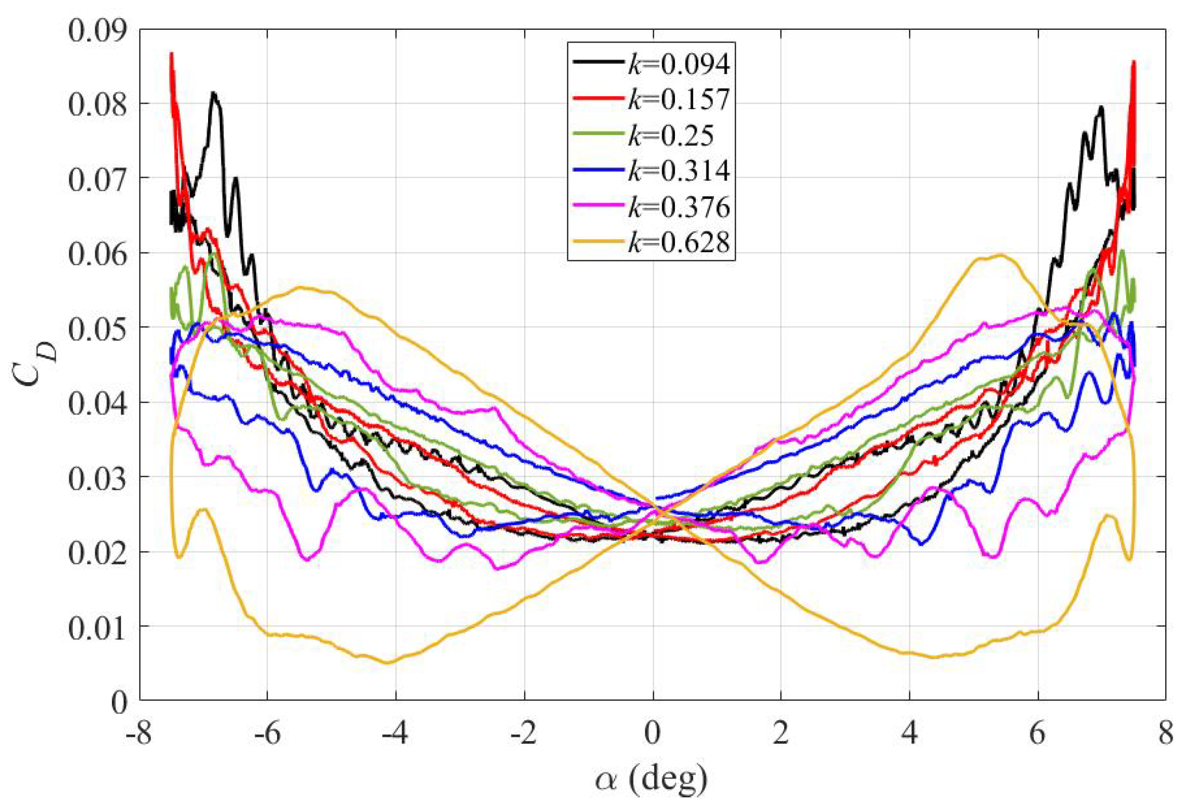
3.1. Aerodynamic Loads

The hysteresis loops of the lift coefficient obtained for different reduced frequencies are presented in Figure 3. With the present pitching amplitude, 7.5°, the pitching angle does not reach the stall angle under the present Reynolds number $6.6\times {10}^4$. The pitching airfoil does not enter the deep stall region, and there is no sudden drop of the $C_l$ curve observed in Figure 3. As the reduced frequency increases from 0.094 to 0.25, in one pitching cycle, the loop has a counter-clockwise circulation direction, and the area closed by the lift coefficient loop shrinks. At $k=0.25$, the lift coefficient changes linearly with the pitching angle, and there is almost no hysteresis loop observed. It suggests that, for a pitching airfoil, although the phase-lag effect is always observed, the hysteresis loop does not necessarily form. It is determined by the operational conditions. As the reduced frequency goes beyond 0.25, the circulation turns to the clockwise direction, and the area closed by the loop increases with the reduced frequency.

The change of the hysteresis loop direction comes with the fact that the lift coefficient at zero incidence has the opposite sign. For cases $k=0.094$, 0.314, and $0.628$, the lift coefficients are $-0.19$, 0.08, and 0.29, respectively. During the first half cycle, the zero-lift of each case is achieved at the pitching angle of $1.0°$ (upstroke), $0.8°$ (downstroke), and $5.0°$ (downstroke), respectively. The instantaneous chordwise distributions of the pressure coefficient at the moment $t=0$ for three cases are shown in Figure 4. With $k=0.094$, the pressure coefficient on the lower side is larger than that on the upper side. As a result, the lower side is the suction side, and the upper side is the pressure side at the corresponding moment. The resultant force in the vertical direction points downwards and has a negative lift, while, with $k=0.314$, the pressure coefficient on the lower side goes beyond that on the upper side after the chordwise position $0.08c$, making the upper side the suction side. Consequently, there is a positive lift for this moment. As the reduced frequency increases to $0.628$, the pressure coefficient on the lower side is larger than that on the upper side almost in the whole chordwise range, resulting in a lift coefficient being 0.29 at this moment.

As the induced frequency increases, the maximum lift coefficient achieved in one pitching cycle decreases. As shown in Figure 5, when the reduced frequency is lower than 0.157, the maximum lift coefficient in one pitching cycle can achieve about 0.698 or slightly lower, which is lower than the lift coefficient for the static airfoil at the corresponding angle of attack. As the reduced frequency goes beyond 0.25, the maximum lift coefficient suddenly drops to 0.52, and it continues to decrease as the reduced frequency further increases. Meanwhile, with a higher reduced frequency, the maximum lift is achieved at a lower incidence (${\alpha }_{Cl,max}$). As the reduced frequency increases from 0.094 to 0.628, the ${\alpha }_{Cl,max}$ decreases from $7.5°$ to $5.2°$ in the upstroke.

The drag coefficient profile, as shown in Figure 6, is also highly dependent on the reduced frequency. As the reduced frequency increases, the maximum drag in one pitching cycle decreases. When the reduced frequency varies between 0.094 and 0.25, the drag coefficient curve in the up- and down-stroke almost overlap with each other, forming small hysteresis loops. As the reduced frequency goes beyond 0.25, the hysteresis loop expands, and the pitching angle at which the maximum drag is achieved decreases. At $k=0.628$, the maximum drag observes at $5.1°$, and it drops suddenly afterwards. The lift and drag coefficients profiles are closely related to the time variation of the instantaneous flow structure near the wall, which will be presented and discussed in the following sections.

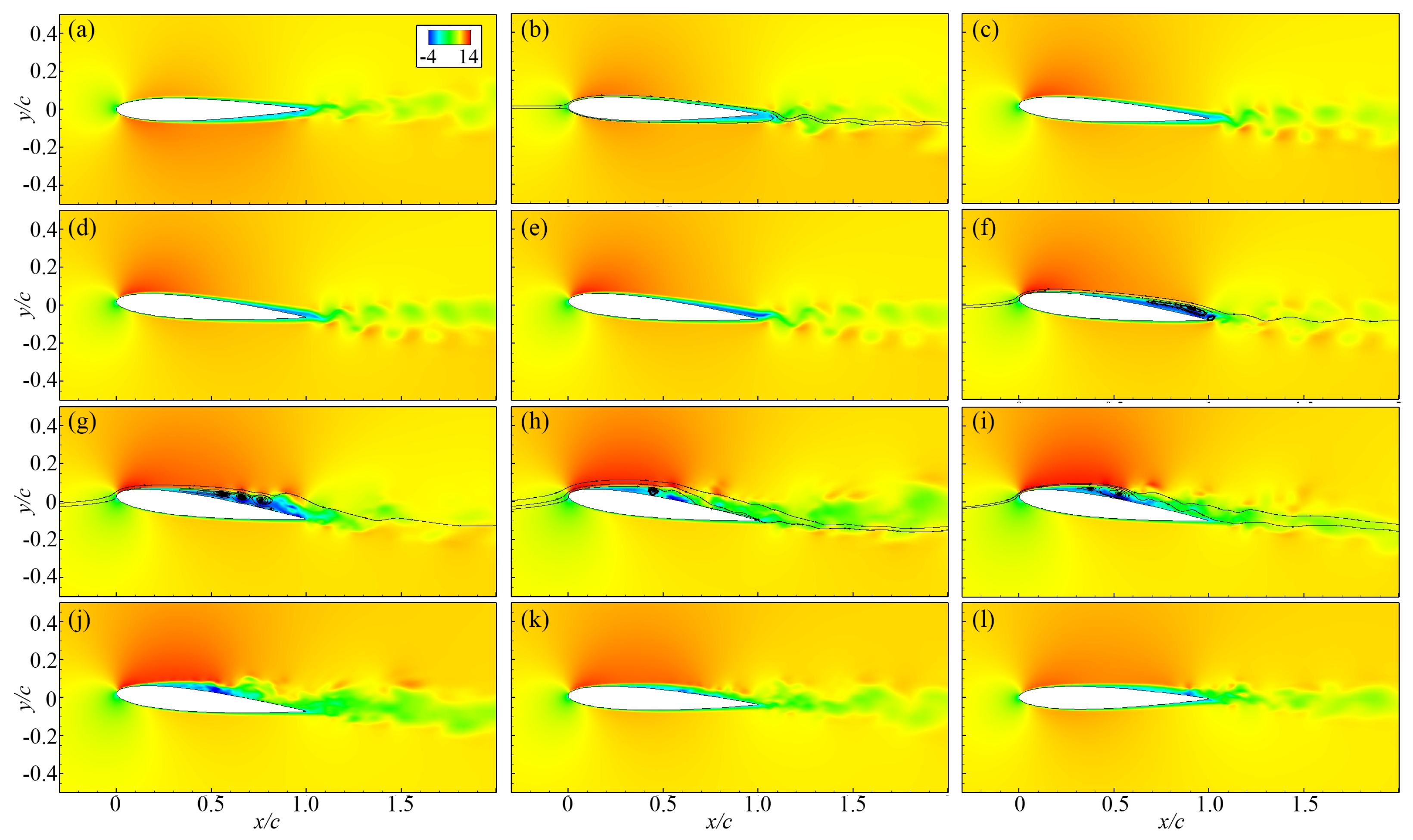
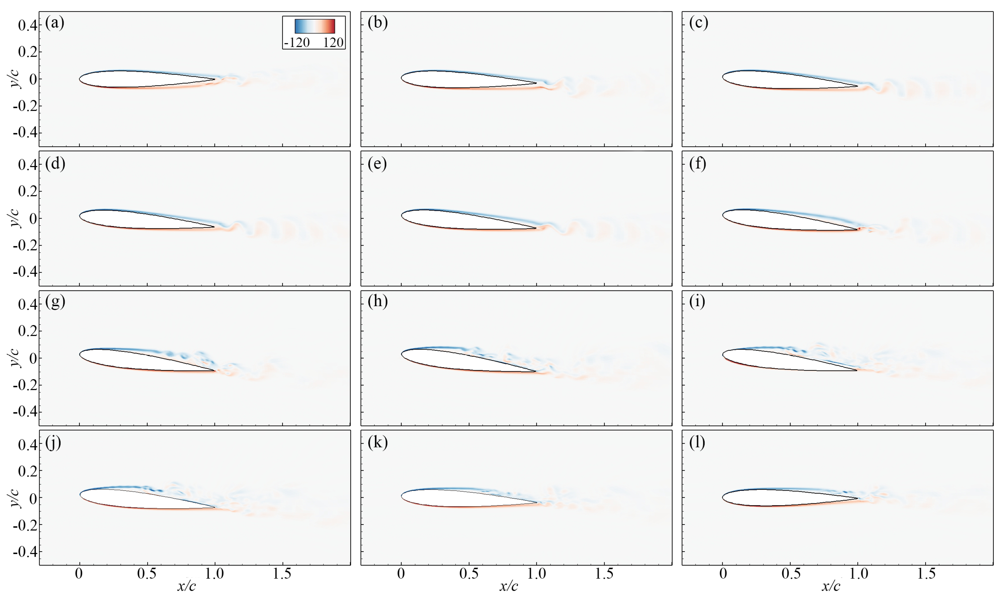
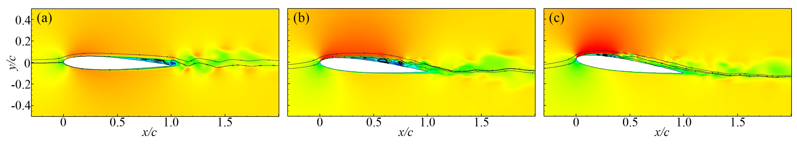
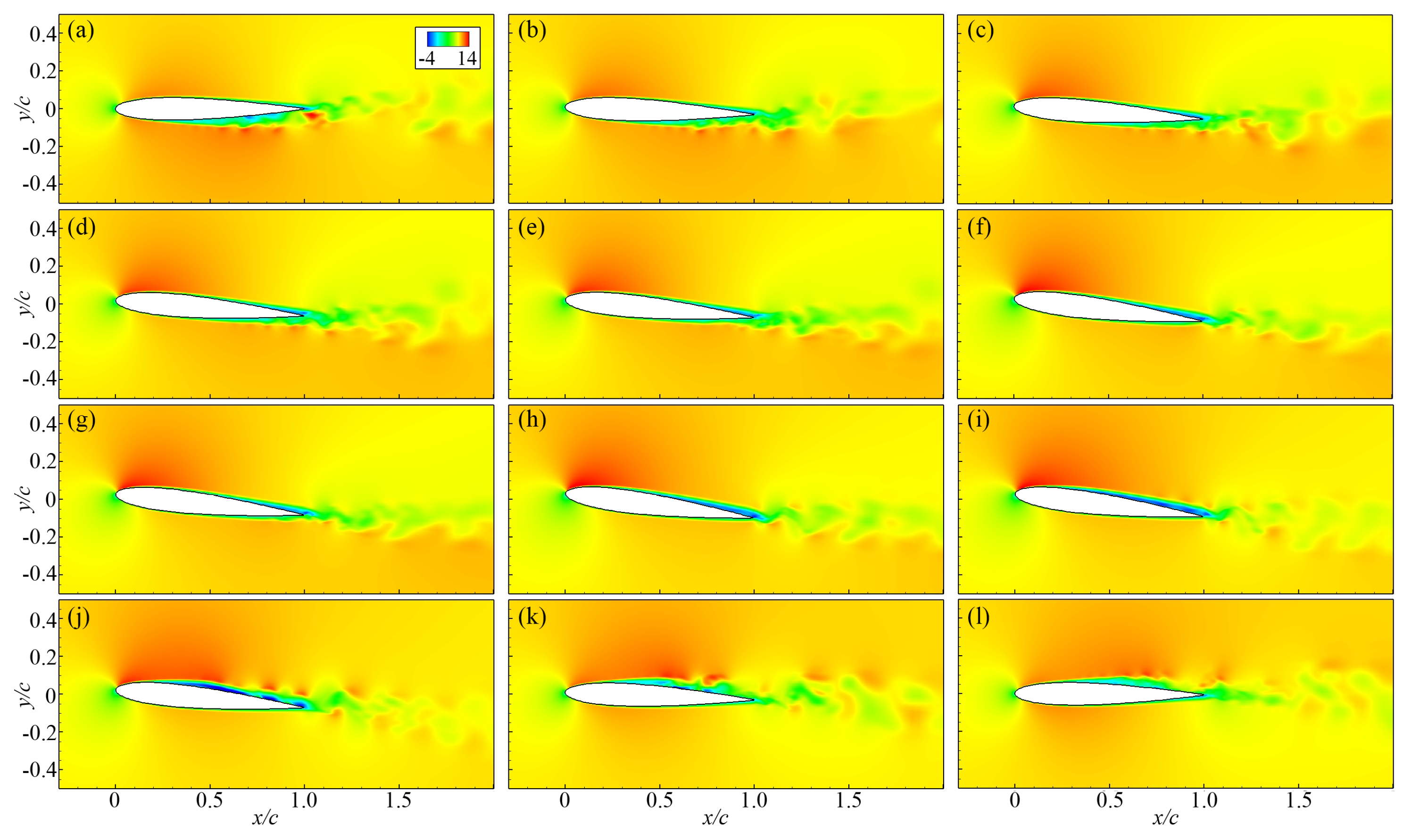
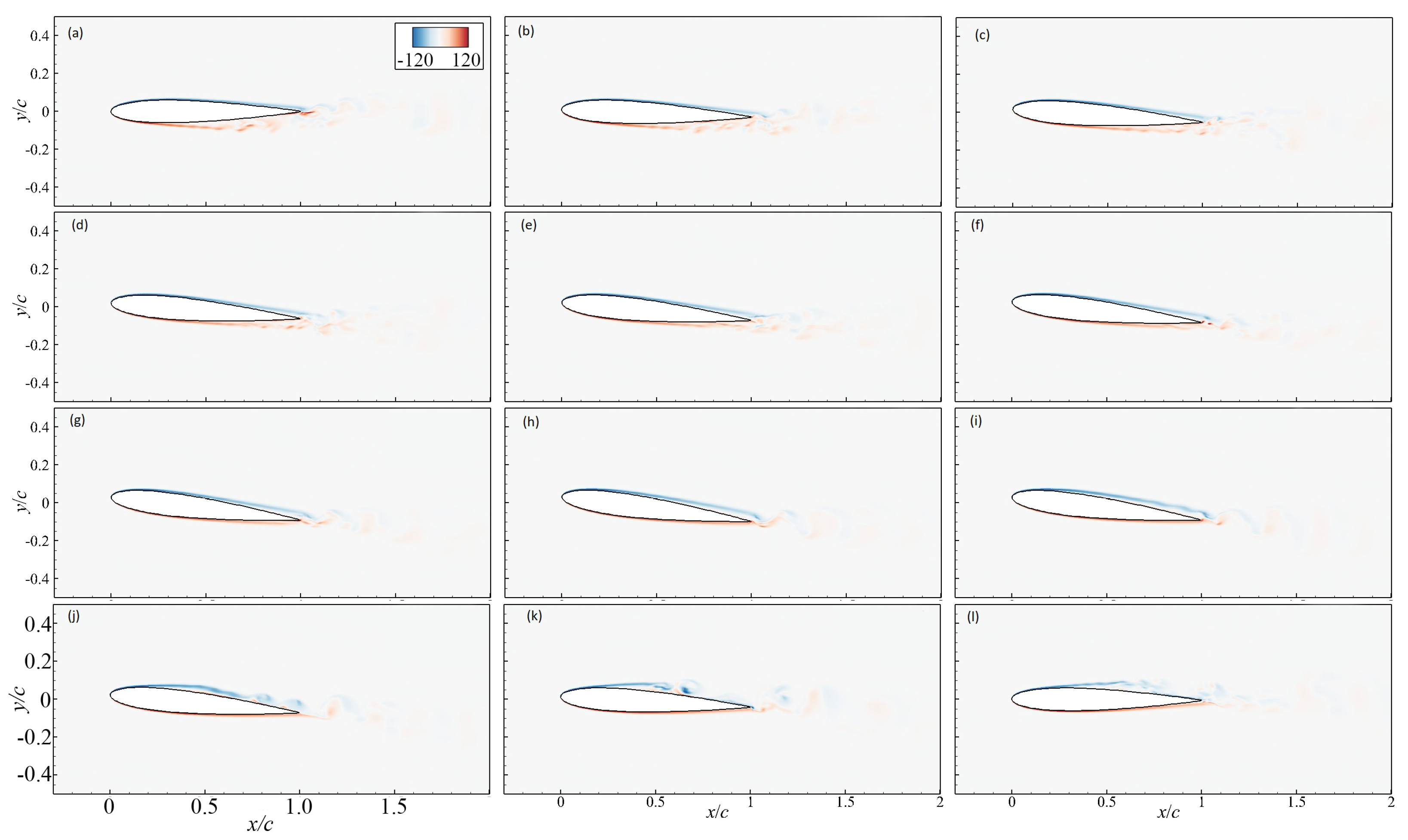
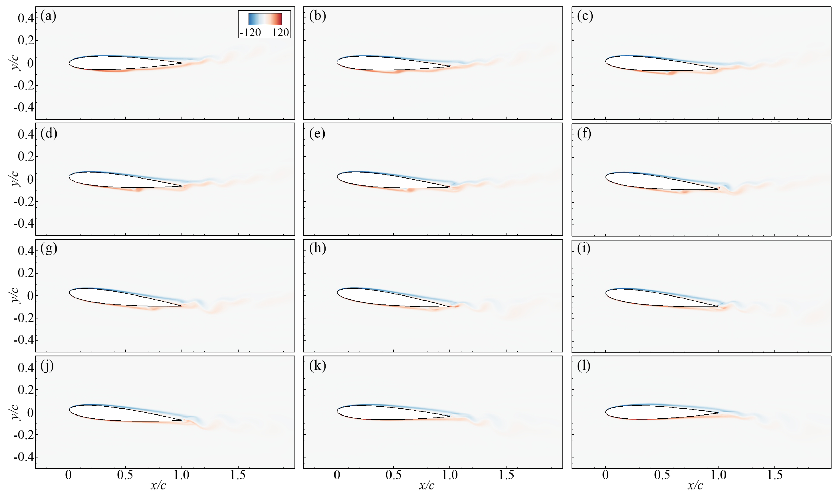
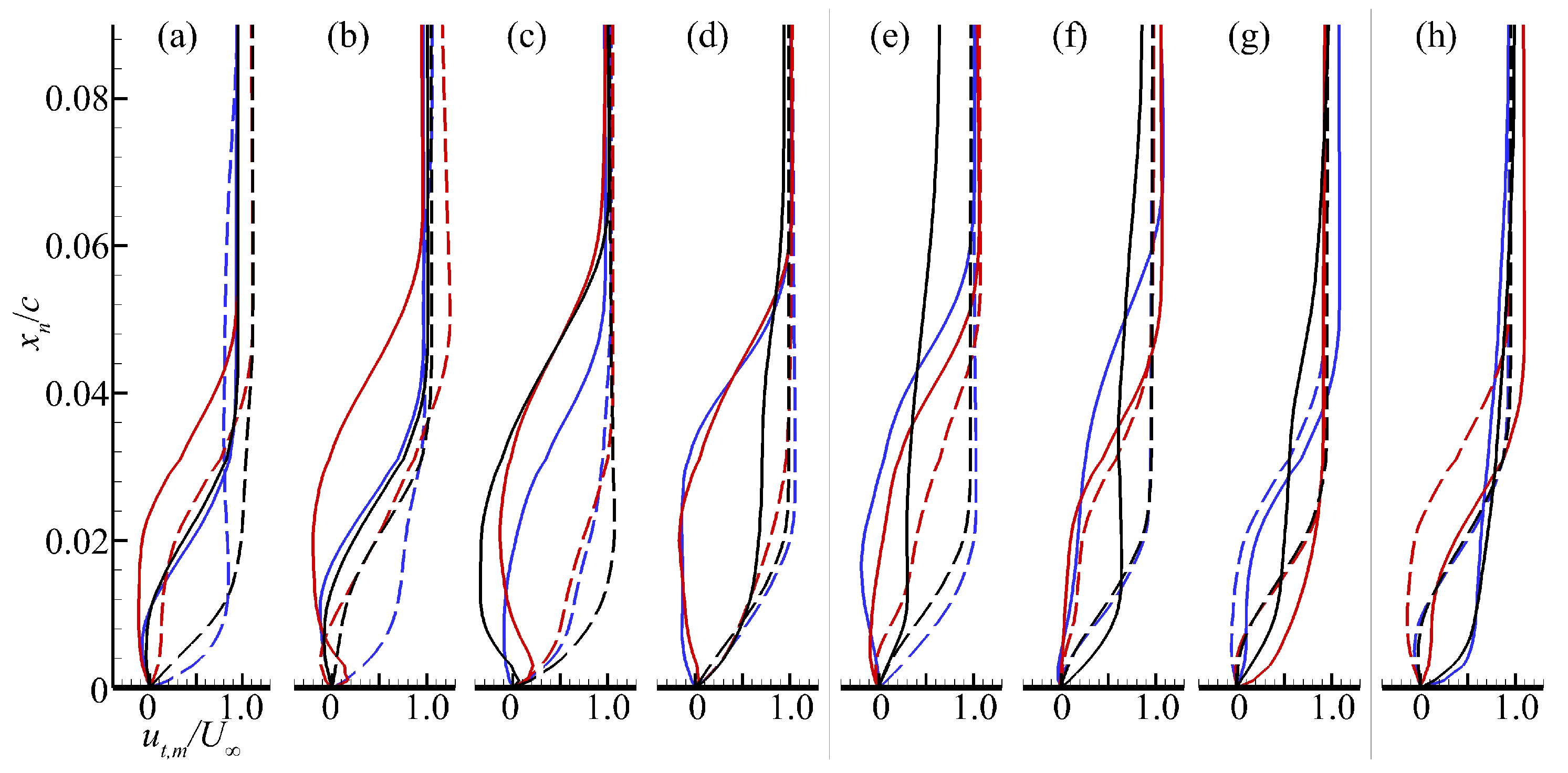
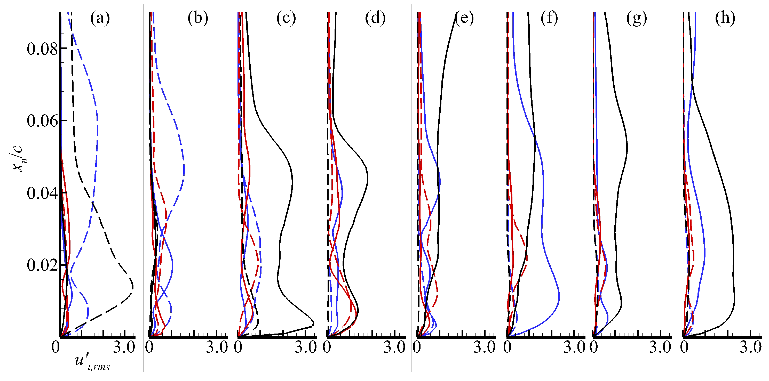
3.2. Flow Pattern near the Pitching Wing

Instantaneous flow patterns for the case with $k=0.094$ are presented in Figure 7 and Figure 8, which are, respectively, coloured by the horizontal velocity component u and the non-dimensional vorticity, which is defined as $\omega c/U_{\infty }$. Since the mean pitching angle is zero and the airfoil features a symmetric profile, only the first half pitching cycle is included. For comparison, the velocity fields obtained from the static airfoil at different angles of attack are given in Figure 9. As shown in Figure 7a–h, in the first quarter pitching cycle, the flow on the lower side remains attached to the wall. On the upper side, the separation point moves from the trailing edge towards the front part as the pitching angle increases, gradually extending the flow separation area. As a result, the region subjected to the negative pressure gradient and reversed flow gradually enlarges. Being different from the static airfoil, the upstroke pitching motion suppresses the flow separation on the upper side. For instance, as shown in Figure 7b and Figure 9a, with the incident angle being $2°$, the region subjected to the reversed flow on the pitching airfoil is much smaller than that on the static airfoil.

As the separation region enlarges, a large-scale coherent structure induced by the reversed flow is present on the upper side near the trailing edge (see Figure 7h, for instance). As the pitching angle increases and the separation point moves upstream, the separation area does not extend infinitely. Instead, the separation vortex breaks into a sequence of vortices as the pitching angle achieves $6.2°$, and the vortex sequence develops into a vortex street at $6.9°$, as shown in Figure 7g and Figure 8g. The vortices are shed from the chordwise position near $0.5c$, and the flow separation point at this moment is $0.24c$. Compared with the static airfoil (as shown in Figure 9b), the vortex street on the pitching airfoil appears at a larger incident angle, while the initiation point of the vortices is located at an upstream position. It should be noted that the incidence at which the vortex street is detected in the present numerical simulation is over $1°$ larger than that observed in the experiments reported by Zhou et al. [23]. This is possibly attributed to the fact that there was no correction applied to the angles of attack referred to in those experiments due to the lack of an effective correction method for the pitching airfoil.

The presence of a vortex street means that a front-part, local flow reattachment occurs, and a separation bubble forms on the front part of the airfoil. Forward flow near the wall is observed right downstream of the first vortex in Figure 7g. This observation agrees well with the flow visualization results reported by Kim and Chang [17], which were acquired using smoke wire technology. As the airfoil approaches the maximum pitching angle, as shown in Figure 7h, flow reattachment occurs in the rear part of the airfoil, the region being downstream of the reattachment point subjected to the turbulent boundary layer. Following that, after $0.25T$, as the pitching angle decreases back to zero, the boundary layer on the upper surface of the trailing edge are maintained in the turbulent state.

Referring to the lift and drag curves presented in Figure 3 and Figure 6, it can be seen that the presence of the vortex street induces increases in both the lift and drag coefficients. In the upstroke stage, as shown in Figure 3, a sudden increase in the $C_l$-$\alpha$ curve slope is observed after $6°$, which is attributed to the presence of the vortex sequence, which prohibits the flow separation. Meanwhile, the large-scale vortex sequence also induces a sudden increase in $C_d$, and the largest $C_d$ reaches the maximum at $6.8°$. Following that, a sudden decrease in $C_d$ occurs, which is attributed to the flow reattachment in the rear part of the airfoil, which leads to the reduction of the separation region.

When $k=0.314$, as shown in Figure 10 and Figure 11, the variation of the flow pattern near the wall shows a different sequence. During the upstroke process, no transition of the boundary layer occurs on the upper side. Only the laminar separation is observed, and the reverse flow region extends towards the leading edge monotonically. Meanwhile, the lower side experiences a transition from the turbulent state to the laminar state. The vortex street on the upper side are observed at $t=0.37T$, at which time the airfoil is in the downstroke process, as shown in Figure 11j. Compared with the vortex street for the case with $k=0.094$, it appears at a later time, has lower strength, and sheds from a more downstream position, $0.65c$. It agrees with the variation trend concluded from experiments [21,23] whereby, as the reduced frequency increases, the time at which the vortex street appears is delayed, and its strength decreases.

As the reduced frequency increases to $0.628$, as shown in Figure 12a and Figure 13a, the upwards deflection of the wake is observed as the airfoil passes the zero-incidence position, which is not seen for cases with lower reduced frequencies. Afterwards, before $t=0.19T_p$, although the airfoil has a positive pitching angle, the wake maintains the upwards deflection, suggesting that, when the reduced frequency is high enough, the wake profile has a hysteresis effect as well. Additionally, during the upstroke process, the laminar flow separation and laminar separation bubble appears simultaneously on the upper and lower sides (see Figure 12a–g), respectively. The laminar separation bubble then moves downstream, and the flow finally re-attaches to the airfoil surface. Note that, as shown in Figure 8 and Figure 11, a shedding of large-scale vortices always occurs on the upper side. As the reduced frequency increases to $0.628$, the separation vortices can only be observed on the lower side.

Comparisons of boundary layer profiles at the trailing edge of cases with $k=0.094$, 0.314, and 0.628 are presented in Figure 14 and Figure 15, in which the phase-averaged tangential velocity ($u_{t,m}/U_{\infty }$) and root mean square of the tangential velocity fluctuation ($u_{t,rms}^{\prime }$) are presented, respectively. It can be seen that the thickening of the boundary layer on the upper side occurs earlier with larger reduced frequencies. Especially when $k=0.628$, the tangential velocity achieves $0.99U_{\infty }$ at $x_n=0.5c$, which is about $0.18c$ larger than that for $k=0.094$ and $0.314$. Additionally, most of the time, the largest velocity fluctuation is obtained with $k=0.094$, and the lowest is always achieved with $k=0.628$. This suggests that increasing the reduced frequency lowers the velocity fluctuations and suppresses the shedding of large-scale separation vortices on the upper side.

Features of the flow structures contribute to the characteristics of the $C_L$ and $C_D$ curves. As discussed above, in one pitching cycle, the lift hysteresis loops for $k=0.094$ and $0.314$ show opposite rotational direction. Consequently, at the moment $t=0$, when the airfoil passes the zero incidence, the lift coefficients of the two cases show opposite signs. As shown in Figure 7a and Figure 10a, at the moment $t=0$, for both cases, the upper side is subjected to the laminar boundary layer separation near the trailing edge, while on the lower side, with $k=0.094$, a laminar separation bubble is observed near the trailing edge, and the local velocity is higher than that on the upper surface, leading to a negative lift; with $k=0.314$, a sequence of separation vortices are observed, generating a large pressure fluctuation (see Figure 4) near the trailing edge, leading to a higher pressure than that on the upper side. Therefore, opposite lift directions are detected for different reduced frequencies.

The phase difference of the near-wall flow structure explains why the maximum lift coefficient decreases as the reduced frequency increases. From the aforementioned load curves and flow patterns, it can be concluded that the lift coefficient at a certain pitching angle is determined by the geometric incident angle and the instantaneous flow structure, which is affected by the pitching frequency. For instance, with $k=0.094$, the vortex street on the upper side is observed at $\alpha =6.2°$, and it is subjected to the turbulent boundary layer as the airfoil achieves the maximum pitching angle, leading to the maximum lift over the whole pitching cycle. As the pitching frequency increases, the presence of the vortex street and hence the turbulent boundary layer is delayed. With $k=0.314$, the turbulent boundary layer on the suction side appears in the downstroke as the airfoil approaches the mean position (see Figure 10k), while at the maximum incidence, the upper side is subjected to the laminar boundary layer separation (see Figure 10h), resulting in a lower lift than that of cases with lower pitching frequencies. As the reduced frequency increases to 0.628, at the maximum incidence, the upper side is still subjected to the laminar boundary layer separation (see Figure 12h), while the lower side observes a small separation bubble causing a decrease in the local pressure. As a result, the lift coefficient at the corresponding moment is lower than that of cases with lower reduced frequencies.

As mentioned above, the pitching motion of the airfoil induces combinations of flow structures on the upper and lower sides that do not present on a static airfoil with the present Reynolds number. A summary of the flow structures on two sides of the airfoil in the first half pitching cycle is given in Figure 16, in which the combinations induced by the pitching motion are marked by the dashed box. With $k=0.094$ and $0.314$, the combinations of laminar separation (upper side) and the laminar separation bubble (lower side) does not occur with a static airfoil. It can only be observed on a static NACA 0012 airfoil when the Reynolds number is as large as $1.6\times {10}^5$ with an angle of attack of $1.5°$ [31]. This implies that the increase in the pitching frequency has a similar effect as increasing the Reynolds number. Furthermore, for a static airfoil, under this Reynolds number, when there is a turbulent boundary layer on the suction side, the pressure side must be subjected to the attached laminar flow, while with $k=0.314$, the laminar boundary layer separation (upper side) and the turbulent boundary layer (lower side) are observed simultaneously. As the reduced frequency increases to $0.628$, at the moment $t=0$, the laminar boundary layer separation and laminar separation bubble are observed simultaneously on the upper and lower side, respectively, which is another phenomenon that is not detected on a static airfoil at the corresponding Reynolds number. This suggests that the effects of the pitching motion not only include the phase lag of certain flow structures, but also are embodied in combinations of flow states that are not observed on a static airfoil.

4. Conclusions and Future Work

Aerodynamic loads and flow structures of a pitching NACA 0012 airfoil were investigated using numerical simulations. The LES approach was employed with the SST turbulence model. All simulations were conducted at a Reynolds number of $6.6\times {10}^4$, and the mean and maximum pitching angles were fixed at $0°$ and $7.5°$, respectively. The effects of reduced frequency are discussed after analyzing and comparing results obtained at $k=0.094$–$0.628$. By examining the load hysteresis, transient variations of flow structures, and boundary layer features near the trailing edge, the following conclusions can be drawn.

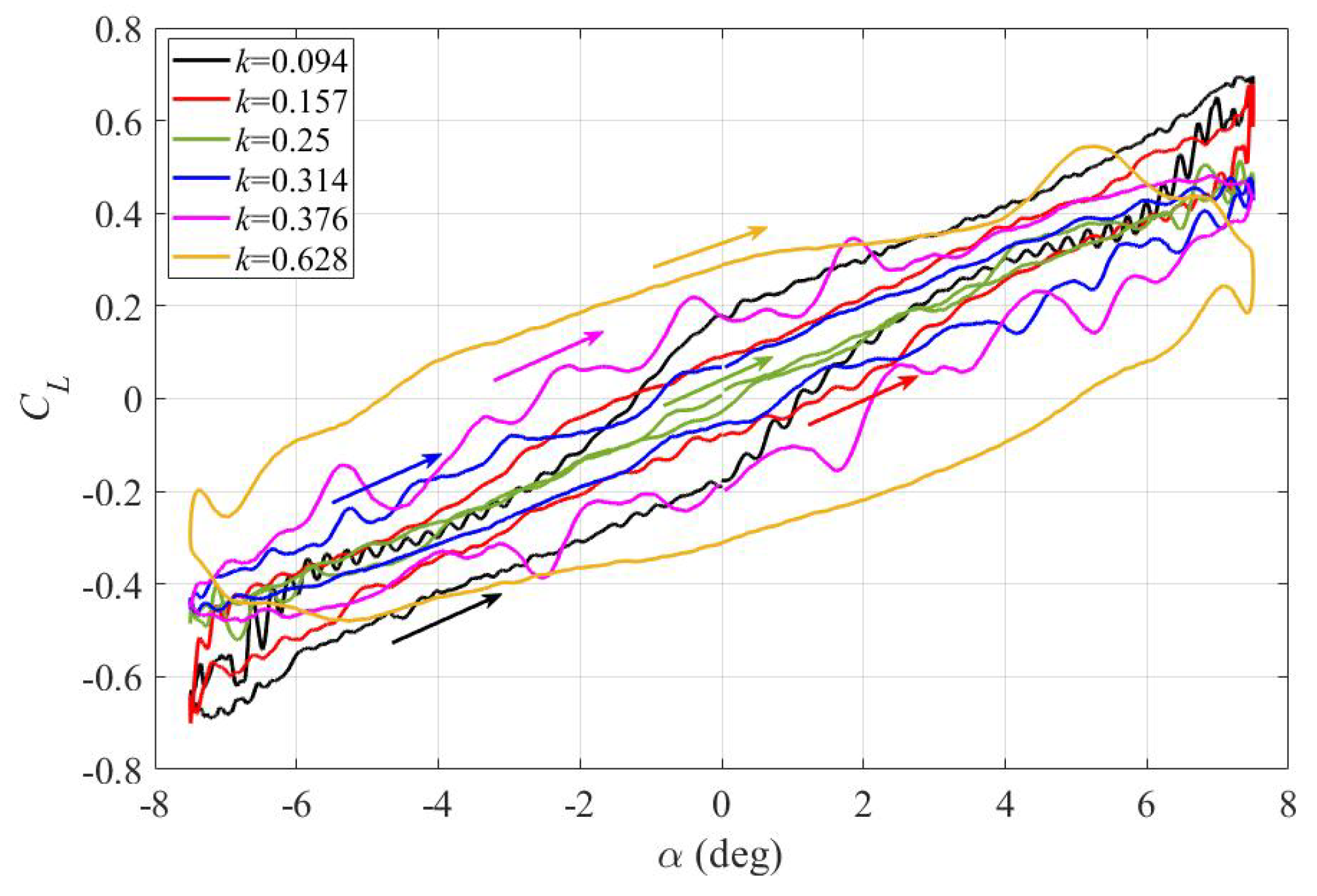
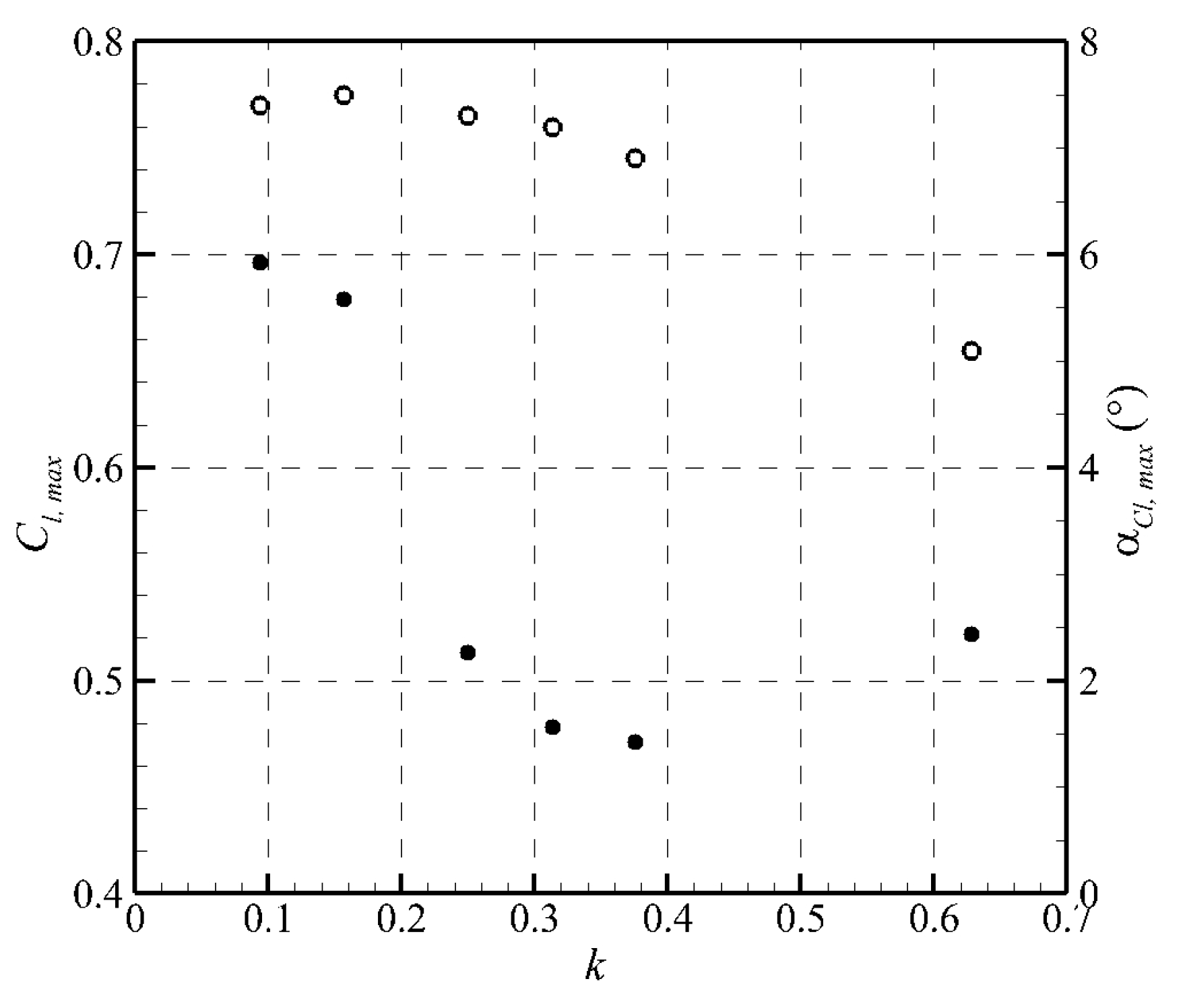
• As the reduced frequency increases from 0.094 to 0.628, the maximum lift coefficient shows a decreasing trend, and the pitching angle at which it is achieved becomes smaller. In one pitching cycle, the circling direction turns from counter-clockwise to clockwise as the reduced frequency exceeds 0.25; consequently, signs of the zero-angle lift coefficient change correspondingly.
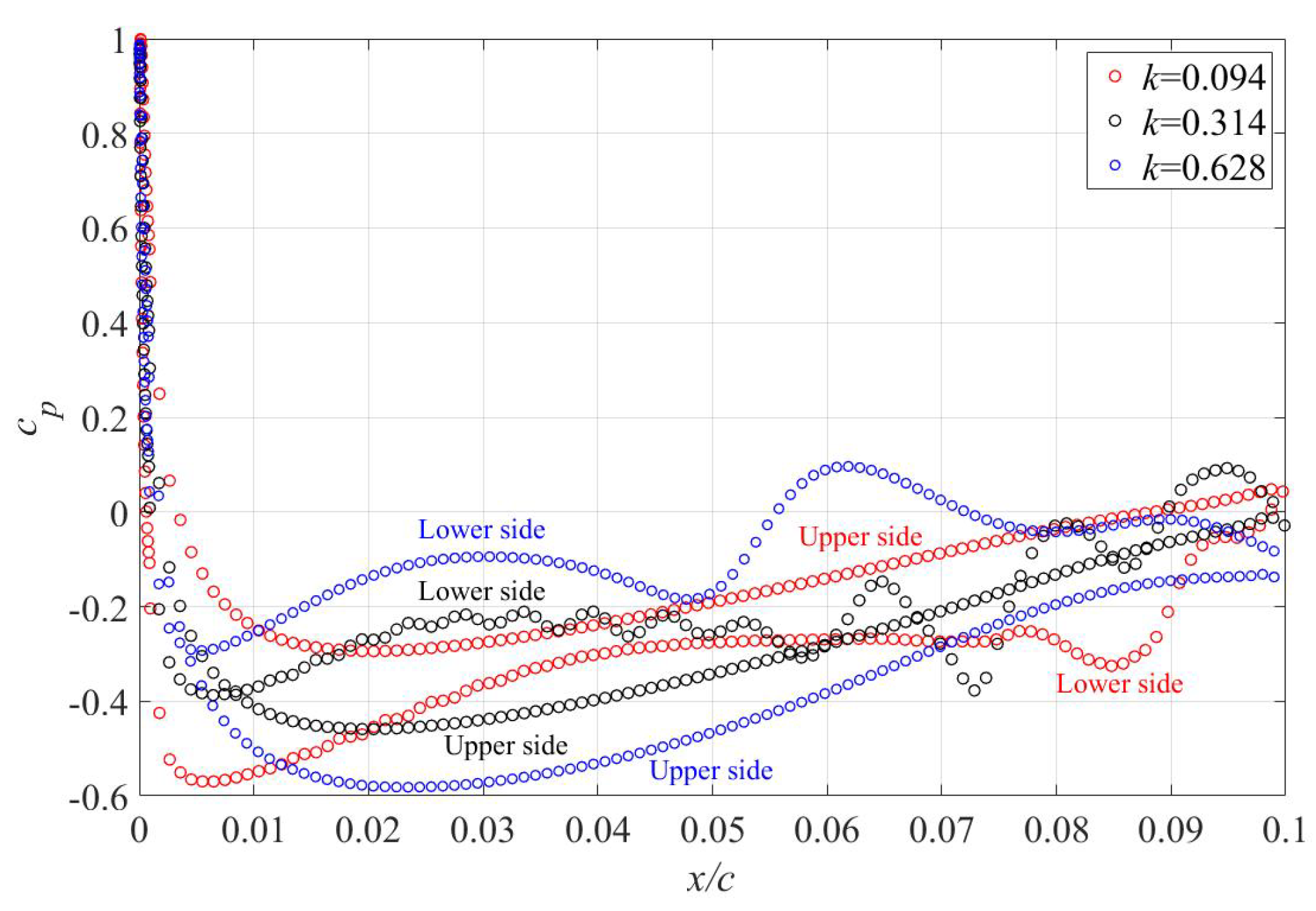
• Besides the phase-lag effect, the pitching motion induces combinations of flow profiles on the upper and lower sides that are not present on a static airfoil at the corresponding Reynolds number, and it is more obvious as the reduced frequency increases. This phenomenon has been rarely reported in previous research. This suggests that the pitching motion not only delays the onset of certain flow patterns, but also induces new observations that are not present on the static airfoil.

This research explores the effects of reduced frequency on the dynamic load and flow structures and the associated boundary-layer features of a pitching airfoil. Results obtained in this research can contribute to the development of more accurate aerodynamic and acoustic prediction models for low Reynolds number airfoils in dynamic stall experiments, and hence help build improved performance prediction models for applications such as propellers in a real operational environment. This will constitute some of the authors’ future research.

References

1. Lee, H.; Lee, D.-J. Rotor interactional effects on aerodynamic and noise characteristics of a small multirotor unmanned aerial vehicle. Phys. Fluids 2020, 32, 047107. [Google Scholar] [CrossRef]
2. Zhao, B.; Li, B.; Cui, W.; Huang, C.; Zhou, T. Approximate entropy identification of flow unsteadiness and surge precursor in both subsonic centrifugal and axial compressors. Phys. Fluids 2025, 37, 027144. [Google Scholar] [CrossRef]
3. McCroskey, W.J.; Carr, L.W.; McAlister, K.W. Dynamic stall experiments on oscillating airfoils. AIAA J. 1976, 14, 57–63. [Google Scholar] [CrossRef]
4. Intaratep, N.; Alexander, W.N.; Devenport, W.J.; Grace, S.M.; Dropkin, A. Experimental study of quadcopter acoustics and performance at static thrust conditions. In Proceedings of the 22nd AIAA/CEAS Aeroacoustics Conference, Lyon, France, 30 May–1 June 2016. [Google Scholar]
5. Knoller, R. Die Gesetze des Luftwiderstandes; Flug- und Motortechnik: Wien, Austria, 1909; Volume 3. [Google Scholar]
6. Betz, A. Ein beitrag zur erklaerung des segelfluges. Z. Flugtech. Motorluftsch. 1912, 3, 269–270. [Google Scholar]
7. Garrick, I. Propulsion of a Flapping and Oscillating Airfoil; Tech. Rep. NACA-TR-567; NACA: Washington, DC, USA, 1937. [Google Scholar]
8. McAlister, K.; Pucci, S.; McCroskey, W.; Carr, L. An Experimental Study of Dynamic Stall on Advanced Airfoil Section; Volume 2: Pressure and Force Data; Tech. Rep. TM-84345-VOL-2; NASA: Washington, DC, USA, 1982. [Google Scholar]
9. Sheng, W.; Galbraith, R.; Coton, F. Prediction of dynamic stall onset for oscillatory low-speed airfoils. J. Fluids Eng. 2008, 130, 101204. [Google Scholar] [CrossRef]
10. Rival, D.; Tropea, C. Characteristics of pitching and plunging airfoils under dynamic-stall conditions. J. Aircr. 2010, 47, 80–86. [Google Scholar] [CrossRef]
11. Carr, L.W.; McAlister, K.W.; McCroskey, W.J. Analysis of the Development of Dynamic Stall Based on Oscillating Airfoil Experiments; Tech. Rep. TN-D-8382; NASA: Washington, DC, USA, 1977. [Google Scholar]
12. Carr, L.W. Progress in analysis and prediction of dynamic stall. J. Aircr. 1988, 25, 6–17. [Google Scholar] [CrossRef]
13. Wernert, P.; Geissler, W.; Raffel, M.; Kompenhans, J. Experimental and numerical investigations of dynamic stall on a pitching airfoil. AIAA J. 1996, 34, 982–989. [Google Scholar] [CrossRef]
14. Sarkar, S.; Venkatraman, K. Influence of pitching angle of incidence on the dynamic stall behavior of a symmetric airfoil. Eur. J. Mech. B Fluids 2008, 27, 219–238. [Google Scholar] [CrossRef]
15. Guillaud, N.; Balarac, G.; Goncalvès, E. Large eddy simulations on a pitching airfoil: Analysis of the reduced frequency influence. Comput. Fluids 2018, 161, 1–13. [Google Scholar] [CrossRef]
16. Negi, P.S.; Vinuesa, R.; Hanifi, A.; Schlatter, P.; Henningson, D.S. Unsteady aerodynamic effects in small-amplitude pitch oscillations of an airfoil. Int. J. Heat Fluid Flow 2018, 71, 378–391. [Google Scholar] [CrossRef]
17. Kim, D.-H.; Chang, J.-W. Unsteady boundary layer for a pitching airfoil at low Reynolds numbers. J. Mech. Sci. Technol. 2010, 24, 429–440. [Google Scholar] [CrossRef]
18. Kim, D.-H.; Chang, J.-W. Low-Reynolds-number effect on the aerodynamic characteristics of a pitching NACA0012 airfoil. Aerosp. Sci. Technol. 2014, 32, 162–168. [Google Scholar] [CrossRef]
19. Kim, D.-H.; Chang, J.-W.; Sohn, M.H. Unsteady aerodynamic characteristics depending on reduced frequency for a pitching NACA0012 airfoil at Rec=2.3×10⁴. Int. J. Aeronaut. Space Sci. 2017, 18, 8–16. [Google Scholar] [CrossRef]
20. Carmichael, B. Low Reynolds Number Airfoil Survey; Tech. Rep. CR-165803-VOL-1; NASA: Washington, DC, USA, 1981; Volume 1. [Google Scholar]
21. Zhou, T.; Sun, Y.; Fattah, R.; Zhang, X.; Huang, X. An experimental study of trailing edge noise from a pitching airfoil. J. Acoust. Soc. Am. 2019, 145, 2009–2021. [Google Scholar] [CrossRef]
22. Zhou, T.; Zhang, X.; Zhong, S. An experimental study of trailing edge noise from a heaving airfoil. J. Acoust. Soc. Am. 2020, 147, 4020–4031. [Google Scholar] [CrossRef]
23. Zhou, T.; Zhong, S.; Fang, Y. Trailing-edge boundary layer characteristics of a pitching airfoil at a low Reynolds number. Phys. Fluids 2021, 33, 033605. [Google Scholar] [CrossRef]
24. Camacho, E.A.; Neves, F.; Silva, A.R.; Barata, J.M. Plunging airfoil: Reynolds number and angle of attack effects. Aerospace 2021, 8, 216. [Google Scholar] [CrossRef]
25. Zhao, M.; Zhao, Y.; Liu, Z.; Du, J. Proper orthogonal decomposition analysis of flow characteristics of an airfoil with leading edge protuberances. AIAA J. 2019, 57, 2710–2721. [Google Scholar] [CrossRef]
26. Zhao, M.; Zhao, Y.; Liu, Z. Dynamic mode decomposition analysis of flow characteristics of an airfoil with leading edge protuberances. Aerosp. Sci. Technol. 2020, 98, 105684. [Google Scholar] [CrossRef]
27. Piomelli, U.; Balaras, E. Wall-layer models for large-eddy simulations. Annu. Rev. Fluid Mech. 2002, 34, 349–374. [Google Scholar] [CrossRef]
28. Cao, H.; Zhang, M.; Cai, C.; Zhang, Z. Flow topology and noise modeling of trailing edge serrations. Appl. Acoust. 2020, 168, 107423. [Google Scholar] [CrossRef]
29. Zhao, M.; Xu, L.; Tang, Z.; Zhang, X.; Zhao, B.; Liu, Z.; Wei, Z. Onset of dynamic stall of tubercled wings. Phys. Fluids 2021, 33, 081909. [Google Scholar] [CrossRef]
30. Miklosovic, D.; Murray, M.; Howle, L. Experimental evaluation of sinusoidal leading edges. J. Aircr. 2007, 44, 1404–1408. [Google Scholar] [CrossRef]
31. Pröbsting, S.; Serpieri, J.; Scarano, F. Experimental investigation of aerofoil tonal noise generation. J. Fluid Mech. 2014, 747, 656–687. [Google Scholar] [CrossRef]
Figure 1. Sketch of the pitching airfoil.
Aerospace 12 00457 g001
Figure 2. Demonstrations of the (a) computational domain and (b) mesh near the airfoil leading edge.
Aerospace 12 00457 g002
Figure 3. Comparison of the C l hysteresis of various reduced frequencies.
Aerospace 12 00457 g003
Figure 4. Comparison of the pressure coefficient profiles at t = 0 for two different reduced frequencies.
Aerospace 12 00457 g004
Figure 5. Dependence of the maximum lift coefficient (solid circles) and incidences at which the maximum lift coefficient is achieved (empty circles) on the reduced frequency.
Aerospace 12 00457 g005
Figure 6. Comparison of the C d hysteresis of various reduced frequencies.
Aerospace 12 00457 g006
Figure 7. Contour maps of the instantaneous horizontal velocity in the first half pitching cycle ( 0 < t < 0.5 T p ) for k = 0.094 . (a) t = 0 T p . (b) t = 0.05 T p . (c) t = 0.09 T p . (d) t = 0.11 T p . (e) t = 0.13 T p . (f) t = 0.16 T p . (g) t = 0.19 T p . (h) t = 0.25 T p . (i) t = 0.31 T p . (j) t = 0.37 T p . (k) t = 0.44 T p . (l) t = 0.49 T p . Contour maps are coloured by u / U .
Aerospace 12 00457 g007
Figure 8. Contour maps of the instantaneous dimensionless vorticity in the first half pitching cycle ( 0 < t < 0.5 T p ) for k = 0.094 . (a) t = 0 T p . (b) t = 0.05 T p . (c) t = 0.09 T p . (d) t = 0.11 T p . (e) t = 0.13 T p . (f) t = 0.16 T p . (g) t = 0.19 T p . (h) t = 0.25 T p . (i) t = 0.31 T p . (j) t = 0.37 T p . (k) t = 0.44 T p . (l) t = 0.49 T p . Contour maps are coloured by ω z * .
Aerospace 12 00457 g008
Figure 9. Contour maps of the instantaneous horizontal velocity of the static airfoil. (a) α = 2 ° . (b) α = 5 ° . (c) α = 7.5 ° . Contour maps are coloured by u / U .
Aerospace 12 00457 g009
Figure 10. Contour maps of the instantaneous horizontal velocity in the first half pitching cycle ( 0 < t < 0.5 T p ) for k = 0.314 . (a) t = 0 T p . (b) t = 0.05 T p . (c) t = 0.09 T p . (d) t = 0.11 T p . (e) t = 0.13 T p . (f) t = 0.16 T p . (g) t = 0.19 T p . (h) t = 0.25 T p . (i) t = 0.31 T p . (j) t = 0.37 T p . (k) t = 0.44 T p . (l) t = 0.49 T p . Contour maps are coloured by u / U .
Aerospace 12 00457 g010
Figure 11. Contour maps of the instantaneous dimensionless vorticity in the first half pitching cycle ( 0 < t < 0.5 T p ) for k = 0.314 . (a) t = 0 T p . (b) t = 0.05 T p . (c) t = 0.09 T p . (d) t = 0.11 T p . (e) t = 0.13 T p . (f) t = 0.16 T p . (g) t = 0.19 T p . (h) t = 0.25 T p . (i) t = 0.31 T p . (j) t = 0.37 T p . (k) t = 0.44 T p . (l) t = 0.49 T p . Contour maps are coloured by ω z * .
Aerospace 12 00457 g011
Figure 12. Contour maps of the instantaneous horizontal velocity in the first half pitching cycle ( 0 < t < 0.5 T p ) for k = 0.628 . (a) t = 0 T p . (b) t = 0.05 T p . (c) t = 0.09 T p . (d) t = 0.11 T p . (e) t = 0.13 T p . (f) t = 0.16 T p . (g) t = 0.19 T p . (h) t = 0.25 T p . (i) t = 0.31 T p . (j) t = 0.37 T p . (k) t = 0.44 T p . (l) t = 0.49 T p . Contour maps are coloured by u / U .
Aerospace 12 00457 g012
Figure 13. Contour maps of the instantaneous dimensionless vorticity in the first half pitching cycle ( 0 < t < 0.5 T p ) for k = 0.628 . (a) t = 0 T p . (b) t = 0.05 T p . (c) t = 0.09 T p . (d) t = 0.11 T p . (e) t = 0.13 T p . (f) t = 0.16 T p . (g) t = 0.19 T p . (h) t = 0.25 T p . (i) t = 0.31 T p . (j) t = 0.37 T p . (k) t = 0.44 T p . (l) t = 0.49 T p . Contour maps are coloured by ω z * .
Aerospace 12 00457 g013
Figure 14. Comparisons of the phase-averaged boundary layer profiles at the trailing edge for different cases. (a) t = 0 T p . (b) t = 0.09 T p . (c) t = 0.16 T p . (d) t = 0.25 T p . (e) t = 0.31 T p . (f) t = 0.37 T p . (g) t = 0.44 T p . (h) t = 0.49 T p . Solid lines: upper side. Dashed lines: lower side. Black: k = 0.094 . Blue: k = 0.314 . Red: k = 0.628 .
Aerospace 12 00457 g014
Figure 15. Comparisons of the root mean squares of the tangential velocity at the trailing edge for different cases. (a) t = 0 T p . (b) t = 0.09 T p . (c) t = 0.16 T p . (d) t = 0.25 T p . (e) t = 0.31 T p . (f) t = 0.37 T p . (g) t = 0.44 T p . (h) t = 0.49 T p . Solid lines: upper side. Dashed lines: lower side. Black: k = 0.094 . Blue: k = 0.314 . Red: k = 0.628 .
Aerospace 12 00457 g015
Figure 16. Combinations of instantaneous flow profiles on the upper and lower sides for cases with different reduced frequencies. LBL: laminar boundary layer. LBLS: LBL separation. TB: turbulent boundary layer.
Aerospace 12 00457 g016