Aircraft Routing and Crew Pairing Solutions: Robust Integrated Model Based on Multi-Agent Reinforcement Learning

Abstract

Every year, airlines invest considerable resources in recovering from irregular operations caused by delays and disruptions to aircraft and crew. Consequently, the need to reschedule aircraft and crew to better address these problems has become pressing. The airline scheduling problem comprises two stages—that is, the Aircraft-Routing Problem (ARP) and the Crew-Pairing Problem (CPP). While the ARP and CPP have traditionally been solved sequentially, such an approach fails to capture their interdependencies, often compromising the robustness of aircraft and crew schedules in the face of disruptions. However, existing integrated ARP and CPP models often apply static rules for buffer time allocation, which may result in excessive and ineffective long-buffer connections. To bridge these gaps, we propose a robust integrated ARP and CPP model with two key innovations: (1) the definition of new critical connections (NCCs), which combine structural feasibility with data-driven delay risk; and (2) a spatiotemporal delay-prediction module that quantifies connection vulnerability. The problem is formulated as a sequential decision-making process and solved via a novel multi-agent reinforcement learning algorithm. Numerical results demonstrate that the novel method outperforms prior methods in the literature in terms of solving speed and can also enhance planning robustness. This, in turn, can enhance both operational profitability and passenger satisfaction.

1. Introduction

In the civil aviation sector, airline planning, including strategic-, tactical-, and operational-level planning, can be a complex and challenging task. Tactical-level planning primarily involves four stages—that is, the schedule design [1,2,3], fleet assignment [4,5,6,7], aircraft routing [8,9,10,11], and crew pairing [12,13,14]. Conventionally, these stages (or problems) are solved in sequence, with each stage’s output serving as the input for the next.

Although the divide-and-conquer method can reduce the complexity of a problem, this modeling approach can lead to a suboptimal solution [15,16,17], particularly for the Aircraft-Routing Problem (ARP) and Crew-Pairing Problem (CPP). The primary source of interaction between the two stages is the change in flight connection time. The buffer time required between two successive flights is not only affected by the minimum sit-time but must also consider whether the crew changes aircraft. For example, when a crew works on two successive flights without changing aircraft, the buffer time between the two flights can be less than the minimum sit-time but must be better than the minimum turn time. These connections are defined as short connections. Consequently, the results of the ARP must be considered when generating crew pairings. However, this sequential approach obtains solutions that are not optimal [18].

Tactical-level plans made before the start of the season are vulnerable to operational disruptions and flight delays that can lead to economic losses for the airlines, as well as damage to their reputations, which can affect their passenger loyalty. Thus, an increasing number of studies have been conducted on the robustness of flight schedules for aircraft and crew [3,9,19,20]. In this context, ‘robustness’ is defined as the ability of a flight plan to suppress the occurrence and propagation of flight delays. Generally, this is quantified by two metrics: (1) the number of flights or flight connections vulnerable to disruptions [21] and (2) the total propagated delay [17,19].

In current research on integrated ARP and CPP, robustness is typically achieved by reallocating buffer time between flights to absorb either non-propagated delays (NPDs) caused by preceding disruptions or anticipated propagated delays. Therefore, how to allocate buffer time effectively between flight connections plays a critical role in schedule robustness. However, overly long or improperly placed buffer times can lead to inefficient schedules, delay propagation, and the reduced utilization of aircraft and crew. Existing methods often rely on static buffer allocation rules, attempting to enhance robustness by extending buffer times across all flight connections indiscriminately. Yet, they lack effective mechanisms for identifying which connections are truly vulnerable to disruptions. As a result, these approaches frequently lead to ineffective or even wasteful buffer time allocation.

Motivated by these gaps, we propose a robust integrated ARP and CPP (RAC) scheduling model aiming to avoid suboptimal decisions and non-robust schedules. First, we design robust policies based on the integrated ARP and CPP characteristics—including buffer time allocation and encouraging the crew to follow the aircraft. Unlike static-rule-based methods, we introduce a data-driven framework that integrates delay prediction and defines new critical connections (NCCs) to identify vulnerable flight links. This enables more targeted and effective buffer time reallocation. Later, we develop the RAC model as a sequential decision-making problem and design a novel reinforcement learning (RL) method to solve the problem. However, the integrated ARP and CPP involve multiple interdependent decision-makers (heterogeneous aircraft fleets and crew groups), each governed by domain-specific rules and restrictions. To address this complexity, we adopt multi-agent reinforcement learning, which enables distributed coordination by decomposing the problem into autonomous agents that optimize their policies while respecting inter-agent dependencies. Finally, extensive computational studies demonstrate that the proposed approach outperforms traditional and heuristic baselines in terms of both solution quality and schedule robustness.

This study is guided by the following key research questions:

(1)

How can flight connections that are truly vulnerable to disruption be systematically identified using data-driven delay prediction?

(2)

How can such predictions be effectively incorporated into a robust and integrated ARP–CPP scheduling model?

(3)

Can a learning-based algorithm efficiently generate resilient aircraft and crew schedules under complex operational constraints?

The remainder of this paper is organized as follows: Section 2 presents a review of the relevant literature; in Section 3, we propose a robust integrated model for the ARP and CPP; Section 4 describes the proposed algorithm designed to solve the model; Section 5 presents the experimental results; in Section 6, we summarize the main contributions of this study and identify meaningful directions for future research.

2. Literature Review

This section reviews research on integrated robust ARP and CPP and RL in airline tactical-level planning problems.

2.1. Robust Integrated ARP and CPP

Over the past decade, extensive studies have focused on integrating the ARP and CPP. Cordeau et al. [22] restricted crew-to-follow aircraft to short connections. Practically, a flight plan in which crew members frequently change aircraft is more likely to suffer from disruptions. Two such cases are illustrated in Figure 1. In the first case, the aircraft from Flight 1 is transferred to Flight 2, and the crew is transferred to Flight 3. If Flight 1 is delayed, Flights 2 and 3 are affected. However, when a crew follows the aircraft (Case 2), only one flight is affected. Consequently, studies have sought to design flight plans in which crews change aircraft infrequently, aiming to enhance the robustness of aircraft and crew scheduling [17,23,24,25]. Table 1 summarizes previous studies on the robust integrated ARP and CPP.

Figure 1. Illustration of crews following aircraft.

Delay absorption (DA) is also used to improve the robustness of aircraft and crew planning. By effectively reallocating buffer time, DA enables the better absorption of disruptions. See Figure 2 for an example.

Figure 2. Illustration of delay absorption.

Dunbar et al. [26,27] proposed a delay propagation formula to accurately estimate and minimize the extra costs owing to propagated delays in a framework that integrated the ARP and CPP. Cacchiani and Salazar-González [28] presented a robust model integrating the fleet assignment problem (FAP), ARP, and CPP. Robustness was ensured by avoiding a short buffer time for the flight connection and penalizing the expected propagated delay. They proposed and compared four heuristic algorithms for solving the model. Ahmed et al. [25] integrated the ARP and CPP by presenting a new polynomial quadratic model. After linearization, their model could be efficiently solved using a commercial solver without the introduction or application of complex Benders’ decomposition or column generation techniques. This study was recently enhanced by Ahmed et al. [17], who integrated the problem with the FAP. Notably, these four seminal studies ensured the robustness of the ARP or CPP by prolonging the connection time between two flights, which was too short to absorb potential disruptions (called critical connections). However, this practice could produce many useless long-buffer connections. Compared to the models proposed by Ahmed et al. [17,25], our approach introduces a delay-prediction-driven mechanism for identifying critical connections and reallocating buffer time more precisely. This enhances the accuracy of buffer management and allows integration with existing airline scheduling systems that handle turnaround planning and crew assignment, thereby improving the model’s practical implementability.

Table 1. Overview of studies on integrated robust integrated ARP and CPP.

Paper	Network	Method to Ensure Robustness	Solving Method
Cordeau et al. [22]	TS	Crews follow aircraft on short connections (CFA)	Benders decomposition
Mercier et al. [18]	TS	Avoid crew changing aircraft on restricted connections (CFA)	Benders decomposition
Weide et al. [23]	SN	Crews follow aircraft on short connections (CFA)	Iterative solution approach
Dück et al. [29]	SN	Minimizing the total propagated delay (DA)	Column generation and dynamic programming
Dunbar et al. [26]	SN	Minimizing the total propagated delay (DA)	An iterative approach
Dunbar et al. [27]	SN	Stochastic versions of Dunbar et al. [26] (DA)	A heuristic algorithm
Ruther et al. [24]	CN	Crews follow aircraft on short connections (CFA)	Dive-and-price
Ahmed et al. [25]	CN	Reward crews following aircraft; penalize connections that are vulnerable to disruptions (CFA and DA)	CPLEX
Cacchiani and Salazar-González [28]	SN	Penalize the expected propagated delay (DA)	Column generation
Ahmed et al. [17]	CN	Penalize the connections that are vulnerable to disruptions and connections crew that do not follow aircraft (CFA and DA)	Proximity search algorithm
This paper	CN	Improved versions of Ahmed et al. [17] (CFA and DA)	Reinforcement learning

Network: Time–space network (TS), connection network (CN), and string network (SN). Method to ensure robustness: Crews follow aircraft (CFA) and delay absorption (DA)

Table 1. Overview of studies on integrated robust integrated ARP and CPP.

Paper	Network	Method to Ensure Robustness	Solving Method
Cordeau et al. [22]	TS	Crews follow aircraft on short connections (CFA)	Benders decomposition
Mercier et al. [18]	TS	Avoid crew changing aircraft on restricted connections (CFA)	Benders decomposition
Weide et al. [23]	SN	Crews follow aircraft on short connections (CFA)	Iterative solution approach
Dück et al. [29]	SN	Minimizing the total propagated delay (DA)	Column generation and dynamic programming
Dunbar et al. [26]	SN	Minimizing the total propagated delay (DA)	An iterative approach
Dunbar et al. [27]	SN	Stochastic versions of Dunbar et al. [26] (DA)	A heuristic algorithm
Ruther et al. [24]	CN	Crews follow aircraft on short connections (CFA)	Dive-and-price
Ahmed et al. [25]	CN	Reward crews following aircraft; penalize connections that are vulnerable to disruptions (CFA and DA)	CPLEX
Cacchiani and Salazar-González [28]	SN	Penalize the expected propagated delay (DA)	Column generation
Ahmed et al. [17]	CN	Penalize the connections that are vulnerable to disruptions and connections crew that do not follow aircraft (CFA and DA)	Proximity search algorithm
This paper	CN	Improved versions of Ahmed et al. [17] (CFA and DA)	Reinforcement learning

Network: Time–space network (TS), connection network (CN), and string network (SN). Method to ensure robustness: Crews follow aircraft (CFA) and delay absorption (DA)

2.2. Reinforcement Learning in Airline Tactical-Level Planning Problems

With the rise of machine learning, studies have begun to apply RL to address airline tactical planning problems—including the FAP, ARP, and CPP.

Ruan et al. [30] successfully designed a heuristic algorithm based on an RL framework to address the ARP. The experiments demonstrated that the proposed algorithm provided better-quality solutions than the genetic algorithm, ant colony optimization, and simulated annealing models. Hu et al. [31] proposed an RL-based method to address aircraft maintenance decisions. Li et al. [32] designed a new algorithm based on an RL framework to address the CPP; the algorithm could produce high-quality solutions for large-scale instances. Thakkar et al. [33] proposed a customer-centric aircraft routing approach integrating dynamic programming and reinforcement learning, introducing a priority assignment mechanism based on customer feedback to prioritize minimizing propagated delays for flights with higher dissatisfaction levels. Evidently, RL-framework-based models can effectively address the tactical-level planning problems of airlines. The RL framework has also been applied to similar optimization problems in civil aviation traffic management. Yuan et al. [34] developed a multi-agent RL-based autonomous interval management system for multi-aircraft scenarios, integrating aircraft performance parameters to enhance both separation assurance and fuel efficiency during en route descent operations. Lee et al. [35] proposed Q-learning and double Q-learning methods for multi-fleet aircraft recovery under severe airline disruptions, showing that RL can flexibly adapt to airline objectives such as minimizing total delays and improving on-time performance using real-world data. Li et al. [36] proposed a real-time airport gate assignment system based on the Asynchronous Advantage Actor–Critic algorithm, integrating flight schedules, gate availability, and passenger walking time into a unified RL framework.

The integrated ARP and CPP can be naturally formulated as a sequential decision-making task with an episodic structure, finite horizon, and well-defined state transitions. These characteristics align with the standard assumptions under which reinforcement learning algorithms are theoretically guaranteed to converge, such as sufficient exploration and bounded returns. In this context, reinforcement learning provides a model-free and flexible framework for optimizing long-term scheduling performance, making it well suited for solving the integrated aircraft and crew planning problems under uncertainty [30,31,32,34]. While prior studies have explored RL applications for the standalone ARP [30,31,33] or CPP [32], these approaches predominantly treat the ARP and CPP as decoupled tasks, overlooking their operational interdependencies. This implies that crew pairing decisions must account for aircraft routing outcomes to ensure schedule feasibility. Sequential or independent optimization methods may lead to suboptimal or even infeasible crew schedules. However, research on integrated flight planning problems through reinforcement learning (RL) frameworks remains scarce. To fill this research gap, this study proposes a novel reinforcement learning (RL) framework to solve the integrated ARP and CPP, explicitly addressing their operational interdependencies.

3. Robust Integrated Model

This study focuses on the RAC model. Here, we first illustrate several concepts and assumptions, followed by a description of notions and the introduction of robustness policies. Finally, we introduce the integrated RAC model.

3.1. Problem Description

The flight scheduling of the airline is divided into two stages [37]. Initially, there is the macro-tactical-level planning of aircraft and crew scheduling for a single season before the season begins. However, within 3–5 days of the actual execution, the airline adjusts or reorganizes the aircraft and crew schedules for the upcoming days (operational-level planning). The primary reason for this reorganization is that pre-established plans may not satisfy maintenance rules or accommodate unforeseen circumstances, such as bad weather conditions or air traffic control. The ARP and CPP examined in this study belong to the second stage, which focuses on the development of robust aircraft and crew schedules for upcoming days based on obtained data regarding potential weather conditions, air traffic control, and other factors. This problem contrasts with creating long-term monthly or seasonal aircraft and crew schedules. Therefore, we develop ARP and CPP models for solving daily periodic flight scheduling problems.

The ARP involves the generation of feasible aircraft rotations that comply with maintenance requirements. Given a set of flights for a specific fleet type, civil aviation authority regulations require maintenance to be performed at airline-designated maintenance workshops after a certain number of flying hours, flight landings, or calendar days [38,39]. The CPP focuses on generating feasible crew schedules that meet safety and labor regulations for duties and pairings. In this context, a duty is defined as a single workday for a crew member that consists of a sequence of flight legs separated by a short rest time. A pairing consists of a consecutive duty period starting and terminating at the same crew base. Two consecutive duties are separated by an overnight rest for the crew [13,14,40].

3.2. Description of Notions

The proposed model is formulated based on a connection network. Let $f\in F$ denote a set of aircraft families. $K^f$ denotes the set of aircraft types belonging to family $f$, indexed by $k$. We can then define the ARP and CPP networks based on the work of Haouari et al. [38], Haouari et al. [40], and Ding et al. [13]. Let $G_k^{ARP}=(V^k,A^k)$ denote the ARP network, where $i \mathrm{a}\mathrm{n}\mathrm{d} j$ represent each node and $(i, j)\in A^k$ represents each arc. Moreover, let $G_f^{CPP}=(V^f,B^f)$ denote the CPP network, where $i \mathrm{a}\mathrm{n}\mathrm{d} j$ represent each node and $(i,j)\in B^f$ represents each arc. The main notation of the ARP and CPP is shown in Table 2 and Table 3, respectively.

Table 2. Notation of ARP.

Sets
$\mathit{P}$	Set of the airport, indexed by $\mathit{p}$
${\mathit{S}}^{\mathit{k}}$	Set of maintenance stations for aircraft of type $\mathit{k}$, indexed by $\mathit{s}$
$\mathit{L}$	Set of legs, indexed by $\mathit{i}$ or $\mathit{j}$
${\mathit{L}}^{\mathit{k}}$	Set of legs that will be served by an aircraft of type $\mathit{k}$, indexed by $\mathit{i}$ or $\mathit{j}$
${\mathit{L}}^{\mathit{f}}$	Set of legs that will be served by an aircraft of family $\mathit{f}$, indexed by $\mathit{i}$ or $\mathit{j}$
${\mathit{L}}_{\mathit{D}}^{\mathit{k}},{\mathit{L}}_{\mathit{D}}^{\mathit{f}}$	A dummy node set of type $k$/family $f$ representing the base where aircraft rotation or crew pairing starts, indexed by 0
${\mathit{L}}_{\mathit{A}}^{\mathit{k}},{\mathit{L}}_{\mathit{A}}^{\mathit{f}}$	A dummy node set of type $k$/family $f$ representing the base where aircraft rotation or crew pairing terminates, indexed by 0
Parameters
${\mathit{t}}_{\mathit{j}}$	The corresponding flying time of flight $\mathit{j}$
${\mathit{D}\mathit{S}}_{\mathit{j}}$	The departure station of flight $\mathit{j}$
${\mathit{A}\mathit{S}}_{\mathit{j}}$	The arrival station of flight $\mathit{j}$
${\mathit{D}\mathit{T}}_{\mathit{j}}$	The departure time of flight $\mathit{j}$ (in minutes)
${\mathit{A}\mathit{T}}_{\mathit{j}}$	The arrival time of flight $\mathit{j}$ (in minutes)
${\mathit{T}}_{\mathit{M}}^{\mathit{k}}$	The time needed to perform the maintenance for aircraft of type $\mathit{k}$
${\mathit{\tau }}^{\mathit{k}}$	Minimum turn time of aircraft of type $\mathit{k}$
${\mathit{N}}^{\mathit{k}}$	Number of available aircraft of type $\mathit{k}$
${\mathit{t}}_{\mathit{m}\mathit{a}\mathit{x}}^{\mathit{k}}$	Maximum flying time between two consecutive maintenance checks of type $\mathit{k}$
${\mathit{\mu }}_{\mathit{m}\mathit{a}\mathit{x}}^{\mathit{k}}$	Maximum times of take-offs between two consecutive maintenance checks of type $k$
${\mathit{d}}_{\mathit{m}\mathit{a}\mathit{x}}^{\mathit{k}}$	Maximum number of calendar days between two consecutive maintenance checks of type $k$
Decision variables
${\mathit{x}}_{\mathit{i}\mathit{j}}$	Binary variable that equals one if arc $(\mathit{i},\mathit{j})\in \mathit{A}$ is selected, and 0 otherwise
${\mathit{u}}_{\mathit{j}}^{\mathit{a}}$	Total accumulated flying hours for an aircraft since its last maintenance check after serving flight $\mathit{j}$
${\mathit{\mu }}_{\mathit{j}}^{\mathit{a}}$	Total accumulated times of take-offs and landings for an aircraft since its last maintenance check after serving flight $\mathit{j}$
${\mathit{d}}_{\mathit{j}}$	Total accumulated number of calendar days for an aircraft since its last maintenance check after serving flight $\mathit{j}$

Table 3. Notation of CPP.

Parameters
${\mathit{s}}_{\mathit{m}\mathit{a}\mathit{x}},{\mathit{s}}_{\mathit{m}\mathit{i}\mathit{n}}$	Maximum and minimum sit-time between two consecutive flights
${\mathit{l}}_{\mathit{m}\mathit{a}\mathit{x}},{\mathit{l}}_{\mathit{m}\mathit{i}\mathit{n}}$	Maximum and minimum layover duration between two consecutive flights
${\mathit{s}}_{\mathit{i}\mathit{j}}$	Denoting the sit-time for crew if and only if $s_{min}\le {DT}_j-{AT}_i\le s_{max}$
${\mathit{l}}_{\mathit{i}\mathit{j}}$	Denoting the layover time for crew if and only if $l_{min}\le {DT}_j-{AT}_i\le l_{max}$
${\mathit{N}}^{\mathit{f}}$	Number of available crews qualified to serve family $f$
${\mathit{t}}_{\mathit{m}\mathit{a}\mathit{x}}^{\mathit{c}}$	Maximum flying time within a duty
${\mathit{\mu }}_{\mathit{m}\mathit{a}\mathit{x}}^{\mathit{c}}$	Maximum number of take-offs within a duty
${\mathit{\lambda }}_{\mathit{m}\mathit{a}\mathit{x}}$	Maximum duty duration
${\mathit{\upsilon }}_{\mathit{m}\mathit{a}\mathit{x}}$	Maximum number of duties within a pairing
${\mathit{\eta }}_{\mathit{m}\mathit{a}\mathit{x}},{\mathit{\eta }}_{\mathit{m}\mathit{i}\mathit{n}}$	Minimum/maximum time away from the base of a pairing
Decision variables
${\mathit{y}}_{\mathit{i}\mathit{j}}$	Binary variable that equals one if $(\mathit{i},\mathit{j})\in \mathit{B}$ is selected, and zero otherwise
${\mathit{z}}_{\mathit{i}\mathit{j}}$	Binary variable that equals one if crew serves the same aircraft on two consecutively flights $i$ and $j$, and zero otherwise
${\mathit{u}}_{\mathit{j}}^{\mathit{c}}$	Total accumulated duty flight duration for a crew since its last layover after serving flight $\mathit{j}$
${\mathit{\mu }}_{\mathit{j}}^{\mathit{c}}$	Total accumulated number of take-offs and landings for the crew since its last layover after serving flight $\mathit{j}$
${\mathit{\lambda }}_{\mathit{j}}$	Total accumulated duty duration for a crew since its last layover after serving flight $\mathit{j}$
${\mathit{v}}_{\mathit{j}}$	Total accumulated number of duties for a crew since its last layover after serving flight $\mathit{j}$
${\mathit{\eta }}_{\mathit{j}}$	Total accumulated time away from base for a crew since its last layover after serving flight $\mathit{j}$

The formation proposed in this paper is an arc-based connection network model. In this network, each node represents a single flight $i$, and each arc $(i,j)$ represents a feasible flight pair that can be chosen. By connecting these flight pairs, feasible sequences of aircraft or crew strings are ultimately formed.

The arc sets $A^k$ and $B^f$ can be divided into several sub-sets:

• ${ A}_1^k:(i,j)\in A_1^k$ if and only if a maintenance check can be performed between ${AT}_i$ and ${DT}_j$, and both $i$ and $j$ are executed the same day by the same aircraft.
• $A_2^k: (i,j)\in A_2^k$ if and only if a maintenance check can be performed between ${AT}_i$ and ${DT}_j$, and $j$ is executed the day after $i$ by the same aircraft.
• $A_3^k:(i,j)\in A_3^k$ if and only if a maintenance check cannot be performed between ${AT}_i$ and ${DT}_j$, and both $i$ and $j$ are executed the same day by the same aircraft.
• $A_4^k:(i,j)\in A_4^k$ if and only if a maintenance check cannot be performed between ${AT}_i$ and ${DT}_j$, and $j$ is executed the day after i by the same aircraft.

Among them, $A_M^k\equiv A_1^k\bigcup A_2^k$ is the set of maintenance arcs; $A_{NM}^k\equiv A_3^k\bigcup A_4^k$ is the set of non-maintenance arcs:

• $B_1^f:(i,j)\in B_1^f$ if and only if the crew that serves family $f$ consecutively serves flights $i$ and $j$, corresponding to the maximum and minimum layover duration.
• $B_2^f:(i,j)\in B_2^f$ if and only if the crew that serves family $f$ consecutively serves flights $i$ and $j$, corresponding to the maximum and minimum layover duration.
• $B_s^f:$ The set of short connections.

Figure 3 illustrates the network of ARP for aircraft type $k$. Assume that the minimum turn time is 30 min. The time needed to perform maintenance is 600 min. Since the base is airport $P$, all arcs departing from airport $P$ belong to $A_{D_p}^k$, and all arcs arriving at airport $P$ belong to $A_{A_p}^k$.

Figure 3. ARP network.

Figure 4 illustrates the network of the CPP for family $f$. Assume that the specified crew sit-time is between 30 and 240 min, and the specified layover time is between 600 and 1200 min. Since the base is airport $P$, all arcs departing from airport $P$ belong to $B_{D_p}^f$, and all arcs arriving at airport $P$ belong to $B_{A_p}^f$.

Figure 4. CPP network.

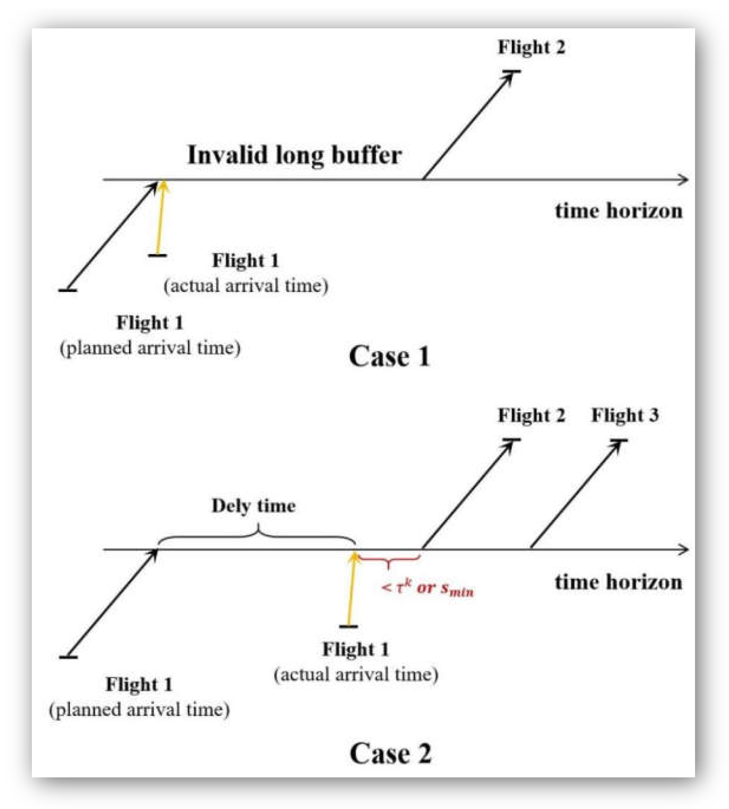
3.3. Robust Policies for ARP and CPP

Ahmed et al. [17,25] applied the buffer time reallocation method to improve scheduling robustness by penalizing flight connections (critical connections) vulnerable to disruption. To explain this, let us first introduce the concept of a critical connection.

Critical connection: This refers to a feasible aircraft or crew connection $\left(i,j\right)$ for which its buffer time, $I_{ij}^k$ or $I_{ij}^f$, is short. For each arc $(i,j)\in A^k$, $I_{ij}^k$ denotes the aircraft’s planned buffer time of arc $(i,j)$, and for each arc $(i,j)\in B_1^f$, $I_{ij}^f$ denotes the crew’s planned buffer time of arc $(i,j)$, which can be expressed as follows:

$$I_{ij}^k={DT}_j-{AT}_i-{\tau }^k$$

(1)

$$I_{ij}^f={DT}_j-{AT}_i-s_{min}$$

(2)

Ahmed et al. [17,25] aimed to absorb potential delays by increasing the buffer time for each connection. However, they did not evaluate the possible delay time for each connection or the ability of the connection to absorb the delay. As a result, the model extended buffer times as much as possible across all connections, rather than prioritizing those with a higher risk of delay. This non-selective allocation ultimately resulted in an ineffective buffer time reallocation. Figure 5 presents the results provided by Ahmed et al. [17,25]. In Case 1, a relatively long buffer time is allocated to the flight connection (1,2). However, as Flight 1 operates on schedule, both the aircraft and crew remain idle on the ground for an extended period, leading to the inefficient use of resources. Case 2 presents a different situation where Flight 1 is delayed. The buffer time for the flight connection (1,2) is insufficient for absorbing this delay, leading to delay propagation for Flight 2. However, the buffer time for the flight connection (1,3) is able to effectively absorb the delay, making it a better scheduling solution. From these two cases, we can conclude that for buffer time re-allocation, it is necessary to (i) avoid excessively long and ineffective long-buffer connections and (ii) ensure that the buffers between flight connections are capable of effectively absorbing delays. Therefore, the accurate prediction of flight delays is crucial for buffer time re-allocation.

Figure 5. Two cases: Results provided by Ahmed et al. [17,25].

In this study, a delay-prediction system is embedded to assess the sensitivity and vulnerability of each connection to disruptions (shown in Appendix B), thereby defining the concept of a new critical connection (NCC).

New critical connection (NCC): This refers to a feasible aircraft or crew connection $\left(i,j\right)$, where the planned buffer time $I_{ij}^k$ or $I_{ij}^f$ is insufficient for absorbing the predicted delay time ${DAT}_i$ of flight $i$. In this study, the possible delay time (${DAT}_i$) can be predicted using a data-driven approach. Formally, an arc $(i,j)\in A_{NC}^k$ if and only if the possible delay time (${DAT}_i$) is larger than the buffer time of the connection and the difference between them is larger than a threshold $I^D$. Thus, an arc $\left(i,j\right)\in A_{NC}^k⟺\left(\mathrm{i}\right){AS}_i={DS}_j;\left(\mathrm{i}\mathrm{i}\right){DT}_j-{AT}_i\ge {\tau }^k;(\mathrm{i}\mathrm{i}\mathrm{i}){DAT}_i-I_{ij}^k>I^D.$ Moreover, an arc $(i,j)\in B_{NC}^f$ if and only if the possible delay time (${DAT}_i$) is larger than the buffer time of the connection and the difference between them is larger than a threshold $I^D$. Thus, an arc $\left(i,j\right)\in B_{NC}^f⟺(\mathrm{i}){AS}_i={DS}_j;(\mathrm{i}\mathrm{i}){DT}_j-{AT}_i\ge s_{min};(\mathrm{i}\mathrm{i}\mathrm{i}) {DAT}_i-I_{ij}^k>I^D.$ The threshold $I^D$ is set as the 95th percentile (P95) of the distribution of ${DAT}_i-I_{ij}$ (historical deviations between predicted delays and buffer time) to ensure robustness while avoiding over-conservatism. This balances the coverage of 95% of delay scenarios with resource efficiency, thereby avoiding over-reservation for the extreme 5% of tail-end delays [41,42,43].

Robustness objective: When an NCC is chosen as the decision for aircraft rotation, the objective function is punished by $p_{ij}^k$, and when an NCC is chosen as the decision for crew pairing, the model incurs a penalty of $p_{ij}^f$. $p_{ij}^k$ and $p_{ij}^f$ can be defined as follows:

$$p_{ij}^k=\left\{\begin{array}{c}{({DAT}_i-I_{ij}^k-I^D)}^2, if (i,j)\in A_{NC}^k\\ 0,otherwise\end{array}\right.$$

(3)

$$p_{ij}^f=\left\{\begin{array}{c}{({DAT}_i-I_{ij}^f-I^D)}^2, if (i,j)\in B_{NC}^f\\ 0,otherwise\end{array}\right.$$

(4)

According to the discussion in Section 2.1, the connection that allows the aircraft and crew to remain together can effectively suppress delay propagation [41,42,43]. Specifically, it suggests that a single flight delay can cause no more than one subsequent delay, whereas separating the crew and aircraft may lead to delay propagation relative to two subsequent flights. Therefore, if an NCC is chosen but the crew does not change aircraft on this connection, the objective function will receive a compensatory reward ${\rho }_{ij}=p_{ij}^f$. This implies the elimination of penalties for delays in subsequently assigned flights caused by crew reassignment to different aircraft [17,25]. For flight connections that do not belong to the set of new critical connections, a fixed reward ${\rho }_{ij}=\overline{\rho }$ will be collected if the aircraft and crew remain together on the connection. Here, $\overline{\rho }$ is a fixed value related to the average flight delay. The reward ${\rho }_{ij}$ can be defined as follows:

$${\rho }_{ij}=\left\{\begin{array}{c}{p}_{ij}^f,if (i,j)\in A_{NC}^k\cup B_{NC}^f\\ \overline{\rho },otherwise\end{array}\right.$$

(5)

3.4. A Nonlinear MIP Formulation for RAC

In this study, we develop an RAC model (Model II) based on the model in Ahmed et al. [17,25] (Model I). Model II can be expressed as follows:

$$max\sum _{(i,j)\in A^k\cup B^f}{\rho }_{ij}{z}_{ij}-\sum _{(i,j)\in A_{NC}^k}{p}_{ij}^k{x}_{ij}-\sum _{(i,j)\in B_{NC}^f}{p}_{ij}^f{y}_{ij}$$

(6)

The objective function (6) involves the penalty of the NCC and the reward for the crew following the aircraft. For the first part, a prize ${\rho }_{ij}$ is granted to each connection where the crew follows the aircraft. In the second two parts, the NCC is penalized by $p_{ij}^k$ and $p_{ij}^f$.

To obtain a feasible solution, the model must satisfy the following aircraft routing and crew pairing constraints. Aircraft routing constraints include flight connections, aircraft capacity, flow conservation, and maintenance feasibility requirements. Crew pairing constraints include flight connection, crew capacity, flow conservation, and duty/pairing feasibility constraints. In addition, linking constraints related to short connections between the two problems must also be met. For clarity, detailed descriptions of the constraints are provided in Appendix C.

4. The Proposed Algorithm

In this section, the proposed multi-agent RL-based algorithm is introduced. First, RL background details are discussed, after which the process of transforming the RAC model into a problem using a Markov decision process (MDP) framework is presented. Finally, we introduce the proposed multi-agent RL algorithm.

4.1. Background

RL is a field of machine learning that emphasizes how an agent should act in a given environment to maximize cumulative rewards through a continuous trial-and-error-based process [44,45]. It can usually be modeled as an MDP framework. A model-free MDP comprises three basic elements—that is, the state, action, and reward. The MDP is a process in which an agent performs an action based on the state and reward obtained from the environment [46,47]. The Monte Carlo control method is a simple method for solving a model-free MDP. Based on the averaged sample returns, the Monte Carlo control method learns from the completed sequence and updates the value function when all states are traversed.

Considering that the integrated ARP and CPP emphasize the integrity of the sequence decision and the influence between states, we use the Monte Carlo control method to generate a robust flight plan.

4.2. Formulation of RAC as Markov Decision Process

First, we model the RAC as a sequential decision-making problem based on the MDP. Consequently, we can define three elements—that is, the state, action, and reward function—for the new sequential decision-making problem. Notably, the proposed model includes two agents for the aircraft and crew, with the two agents having a completely cooperative relationship.

4.2.1. State Space

The state vector $s_t$can be considered to be the basic information required by the two agents for each action at the decision step $t$. Each state $s_t$ at step t is defined as a composite structure containing two modules: $s_t=({FlightInfo}_t,PreviousAssignment)$. ${FlightInfo}_t$ includes five-dimensional information: the flight departure airport, departure time, arrival airport, arrival time, and flight time. The PreviousAssignment module includes the flight number, the assigned aircraft, and the assigned crew from the previous step $t-1$. Moreover, each element in the set of states can be arranged incrementally according to the departure time of each flight. The two agents transition from the initial state to the terminal state, assigning the aircraft or crew to each state along the way. Whenever a crew-following-aircraft connection or NCC exists, the agent receives corresponding rewards.

4.2.2. Action Space

In the new RAC sequential decision-making problem, the action $a_{s_t}$ represents the behavior of the two agents and assigns the aircraft or crew to the flight state $s_t$ during interactions with the environment at decision step $t$. It is crucial to emphasize that the action space is dynamically constrained by a comprehensive set of rules (Constraints (A6)–(A46)) that encode resource-specific dependencies. These constraints ensure that the decision-making process accounts for the temporal evolution of resource availability.

4.2.3. Reward Function

The reward function and cooperation mechanism of the two agents must be designed according to the objective function and constraints of the RAC model. The reward function $r_t$ denotes the rewards obtained after the aircraft agent and crew agent perform action $a_{s_t}$. Let $(i_a,j_a)$ denote the newly generated flight connection resulting from the completion of action $a_{s_t}$.

$$r_t=\left\{\begin{array}{c}{\rho }_{(i_a,j_a)},if x_{i_a,j_a}=1 and y_{i_a,j_a}=1\\ -p_{(i_a,j_a)}^k,if (i_a,j_a)ϵA_{NCC}^k\\ -p_{(i_a,j_a)}^f,if (i_a,j_a)ϵB_{NCC}^f\\ M,if {\mathbb{I}}_{violate}(a_t)=1\\ 0,otherwise\end{array}\right.$$

(7)

where M is a large penalty value. The indicator function ${\mathbb{I}}_{violate}=1$ if and only if aircraft maintenance or crew rules are violated after the completion of action $a_{s_t}$; otherwise, ${\mathbb{I}}_{violate}=0$.

The two agents move continuously from the initial state to the last state and assign the aircraft and crew to each state when meeting the RAC constraints. If an NCC occurs, the two agents receive corresponding negative rewards. If aircraft maintenance is not feasible, the aircraft agent receives the corresponding negative reward. When violating the crew rules, the crew agent receives corresponding negative rewards. Finally, when each state is assigned to the corresponding aircraft and crew, we can determine whether there is an unfeasible short connection or a connection in which the crew can follow the aircraft based on the scheduling results and then assign the corresponding positive or negative feedback. Notably, we first assume that all short connections are selectable. When a short connection occurs but is not feasible, the two agents receive the corresponding negative reward (NR). This negative reward is related to the number of iteration rounds; when the same infeasible short connection occurs in multiple iterations, the crew agent receives a negative reward.

Here, we denote $R_t$ as the reward received in the decision step $t$. The total discounted reward $G_t$ at the decision step $t$ can be expressed as follows:

$$G_t=(R_t+\gamma R_{t+1}+{\gamma }^2{R}_{t+2}+\dots |s_t=s)$$

(8)

where $\gamma$ denotes the discount factor in the process of cumulative positive/negative reward, which determines the importance of immediate feedback versus future feedback under the policy $\pi (s_t,a_{s_t})$. If $\gamma$ is set to 1, the two agents focus more on future rewards. Conversely, if $\gamma$ is set to 0, only immediate rewards are considered. In this paper, $\gamma$ is set to 1 to maximize the total cumulative rewards.

There may be multiple actions ($a_{s_t}$) when selecting an aircraft or crew for state $s_t$. Thus, to find the optimal policy $\pi (s_t,a_{s_t})$, it is necessary to generate state action evaluation value functions $Q(s,a_s)$, as shown in Equation (9), and determine the optimal policy ${\pi }^{best}(s)$ using Equation (10). It should be noted that the optimal action in each state must satisfy the aircraft maintenance and crew constraints in Appendix C.

$$Q_{\pi }(s,a_s)=(\sum _{i=0}^{\infty }{\gamma }^i{R}_{t+i}|s_t=s,a_t=a_s)$$

(9)

$${\pi }^{best}(s)=arg{max}_{a}Q(s,a_s)$$

(10)

Here, we can use the $\epsilon$-greedy policy to select the current optimal action. This implies that the agent has a high probability of choosing the action with the maximum Q value, but the agent has probability $\epsilon$ when choosing a random action. The goal of this method is to encourage the agent to select more random policies during the early stages of learning to promote initial exploration. For details, see Equation (11).

$$a(s)=\left\{\begin{array}{c}arg{max}_{a}Q(a,a_s), \forall random(\mathrm{0,1})\le 1-\epsilon \\ random{a}_s, \forall random(\mathrm{0,1})>1-\epsilon \end{array}\right.$$

(11)

The RAC model is solved in parallel for the entire aircraft family; hence, for aircraft family $f$, the flights that each subfleet needs to execute are fixed in advance by the FAP, whereas the crews for family $f$ need to execute the flight of each subfleet. The framework of the proposed algorithm for a single aircraft family is as shown in Figure 6. For a single aircraft family $f$, the aircraft agent is divided into several subagents to generate aircraft rotation. Meanwhile, the crew agent needs to generate schedules for the crew qualified for these aircraft types. The two types of agents share global information, generate feasible flight strings in parallel, collect rewards, update the Q value table, and return to iterations.

Figure 6. Framework of proposed algorithm (RL) for a single aircraft family.

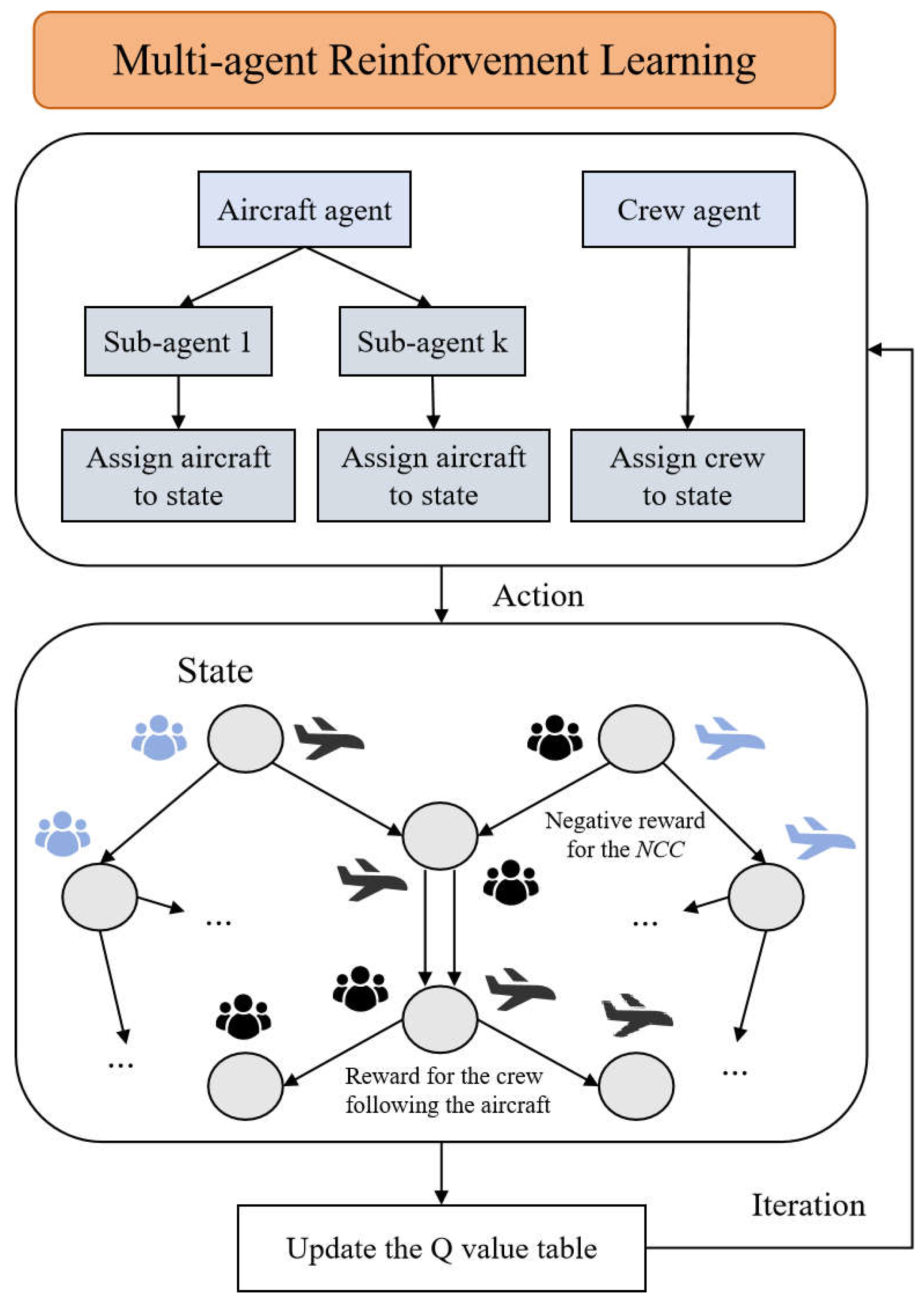
4.3. Reinforcement Learning-Based Algorithm

In this study, we propose an algorithm based on the MDP framework for the RAC model and the work of Lee et al. [48] and Ruan et al. [21]. Here, we define three new lists as follows:

$FL$: A list containing details of flight legs.

${AN}^k$: A list containing the tail numbers for subfleet $k$.

${CN}^f$: A list containing the number of crews that can execute family $f$.

We split ${AN}^k$ into three sublists—that is, ${IU}_a^k$, ${NIU}_a^k$, and ${IM}_a^k$. Here, the sublist ${IU}_a^k$ denotes the list of aircraft used, ${NIU}_a^k$ denotes the list of available aircraft, and ${IM}_a^k$ denotes the list of aircraft in maintenance. The same split can be created for ${CN}^f$. Here, sublist ${IU}_c^f$ denotes the list of crew members on duty, ${NIU}_c^f$ denotes the list of available crews, and ${IL}_c^f$ denotes the list of crews with a layover. To ensure robustness, we create four empty lists—that is, normal flight connections (${FC}_a^k$ and ${FC}_c^f$) and non-NCCs ($N-{NCC}_a^k \mathrm{a}\mathrm{n}\mathrm{d} N-{NCC}_c^f$). Finally, we prepare the Q value table, where each element in the table indicates the value of choosing action $a_{s_t}$.

Start to formulate a reinforcement learning policy. The agents constantly allocate aircraft and crew to the state and follow these steps until the terminal flight’s completion:

Step 1: If the list $IU$ or $FC$ is empty, assign the first aircraft/crew in list $NIU$ to its current state, delete the aircraft/crew from $NIU$, and add it to the $IU$. Then, move to the next stage and check whether any aircraft/crew in $IM/IL$ has completed maintenance/layover operations. If so, move them from $IM/IL$ to $NIU$ for subsequent selection, and move to Step 2.

Step 2: If $IU$ is not empty, check whether there are aircraft/crew in list $IU$ that meet Constraints (A6)–(A41). If present, add all aircraft/crew that satisfy the constraints to $FC$ and proceed to Step 3. If no aircraft/crew satisfy the constraints, return to Step 1 for reselection. Moreover, if any aircraft does not meet the maintenance constraints, it is deleted from $IU$ and added to $IM$. The maintenance visit is then arranged based on the arc set $A_M^k$ and provides a negative reward when there is any unavoidable infeasible maintenance. Meanwhile, if any crew does not meet the work-rule constraints, it is deleted from $IU$ and added to $IL$. The layover visit is then arranged based on the arc set $B_2^f$ and provides a negative reward when there is any unavoidable infeasible layover.

Step 3: If $FC$is not empty, check whether there are any aircraft/crew in $FC$ that are non-NCCs. If yes, remove them from the $FC$ and add them to the $N-NCC$ and move to Step 4. If not, proceed to Step 5.

Step 4: If there are any non-NCCs, the agents select the aircraft/crew with the highest current Q value from $N-NCC$ with a probability of 1 − $\epsilon$ or randomly select an aircraft in $IU$with probability $\epsilon$ and assign it to the current state. Subsequently, the agents receive the corresponding reward. Move to the next state and update lists $IU$ and $NIU$. Reset $FC$ and $N-NCC$, and return to Step 1. If this is the last state, proceed to Step 6.

Step 5: If there are only NCCs, the aircraft/crew agent selects the aircraft with the maximum current Q value from $FC$ with probability 1 − $\epsilon$ and receives a negative reward for the NCC or randomly selects the first aircraft/crew from $FC$ or $NIU$ with probability $\epsilon$ and assigns it to the current state. Move to the next state and update lists $IU$ and $NIU$. Reset $FC$, and return to Step 1. If this is the last state, proceed to Step 6.

Step 6: If the agents traverse from the first flight state to the last state, they move to the Q value table’s update stage.

Update of Q Value Table

After the aircraft and the crew agents have completed a round of state action selection, the algorithm checks for any infeasible short connections or valid crew-following-aircraft connections and assigns corresponding positive or negative rewards to the two agents. Calculate the cumulative reward $G_e$ for this round. $G_e$ is the cumulative reward based on state $s$ and action $a_s$. To improve the convergence speed, $G_e$ is computed using different strategies depending on the round index, as shown in Equations (12)–(14):

$$G_e(s,a_s)=\left\{\begin{array}{c}{\displaystyle \sum _{t=1}^{t=T}}{r}_t, 0\le e\le E_2,\\ {\displaystyle \sum _{t=1}^{t=T}}{r}_t-G_{average}, E_2\le e\le E_1.\end{array}\right.$$

(12)

$$G_{average}={\displaystyle \frac{{\sum }_{e=1}^{e=E_2}{\sum }_{t=1}^{t=s}{r}_t}{E_2}}$$

(13)

$$Q(s,a_s)=Q(s,a_s)+\alpha (G_e-Q(s,a_s))$$

(14)

where $E_1$ denotes the maximum allowable number of rounds set by the algorithm, $E_2$ denotes the number of intermediate rounds set to accelerate the convergence of the algorithm, and $T$ denotes the total number of time steps in an episode. Accordingly, update the Q table based on Equation (14), where $\alpha$ denotes the independently set learning rate. If the algorithm reaches the set maximum allowable number of rounds ($E_1$), the iteration is terminated, and the final flight plan is generated. The learning rate $\alpha$ is set to 0.1 if $G_{e+1}\le G_e$ and 0.2 otherwise.

5. Computational Results and Discussion

In this section, we compare the results provided by Model I (the model proposed by Ahmed et al. [17,25]) and Model II (the model proposed in this study). We use the proposed RL-based algorithm to solve these two models.

5.1. Comparison Method

We compare the performance of the RL-based algorithm with sophisticated methods for solving the integrated ARP and CPP, such as CPLEX, the Proximity Search Algorithm (PSA), and the column generation algorithm-based method (CG-B), as proposed in recent works [13,15,17,25,28]. To avoid making the paper overly lengthy, the details of the methods are presented in Appendix A. All computational experiments are carried out on an Intel Core i7-8750H CPU-based platform running at 2.20 GHz with 16 GB of RAM, without GPU acceleration. For the largest instance tested, the model converges within 1800 episodes, with a total training time of approximately 2.4 h on this standard CPU platform.

5.2. Data Introduction

The ARP and CPP examined in this study do not involve the macro-level scheduling of aircraft and crew (further details are provided in Section 3.1), where plans are made six months prior to the start of a season. Instead, these problems focus on rescheduling aircraft and crew for the upcoming days based on anticipated irregular conditions that may occur prior to macrolevel planning (3–5 days prior). Therefore, we chose a three-day schedule to perform robustness testing on the models. The flights in this schedule are repeated daily with minor differences each day. The input data for the RAC model include four instances (Table 4), and the largest instance includes 1239 flights. The primary dataset used in this study is provided by a partner airline through a research collaboration agreement.

Table 4. Description of the instances.

Instance		Aircraft			Short Connection
	Family	Aircraft Type	Aircraft	Flights
Instance I	A320	A320	8	40	5
Total	1	1	8	40	5
Instance II	A320	A320	12	110	24
	BAE	BAE200	5	53	9
Total	2	2	17	162	33
Instance III	F100	F100	18	99	33
	ERJ170	ERJ170	6	39	10
		ERJ190	10	82	12
	A320	A320	32	456	90
Total	3	4	66	676	145
Instance IV	ERJ145	ERJ135	5	36	9
		ERJ145	8	78	6
	CRJ	CRJ100	7	72	9
		CRJ700	5	42	6
	BAE	BAE200	5	39	9
		BAE300	5	72	4
	A320	A319	30	312	64
		A320	42	477	123
		A321	12	111	6
Total	4	9	119	1239	236

We collect air route data, historical delay records, weather conditions, and air traffic control data (from VariFlight) relevant to the four instances for a single season. We group these data into different datasets based on a three-day cycle and selected six datasets. Then, we expand the Test Case into six groups by incorporating different irregular event data (six data sets), labeled as Test Case (1), Test Case (2), ..., Test Case (6). Subsequently, we use a data-driven approach to predict the potential arrival delays for each flight. The details are presented in Appendix B. We build the sets of NCCs for each flight in the Test Case (1)–Test Case (6).

To account for the maintenance feasibility of the ARP, duties, and pairing legacy for the CPP, we set the corresponding parameters based on the literature. In general, each fleet type has its own requirements between two consecutive A-checks.

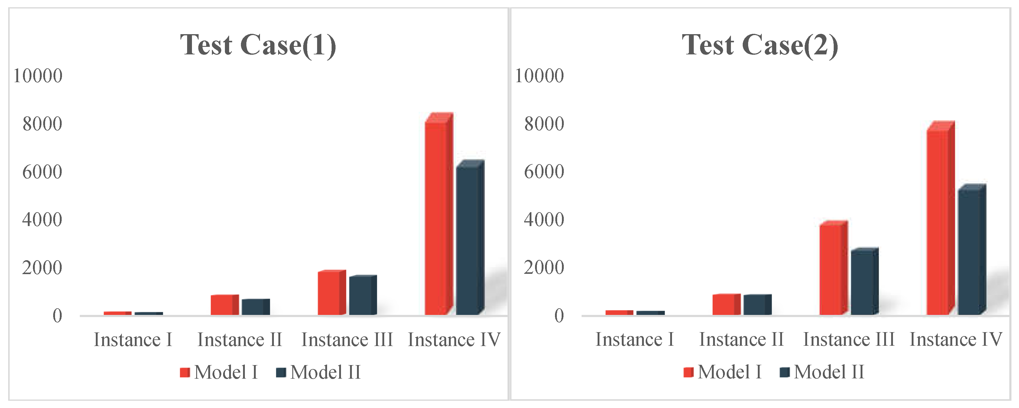
5.3. Robust Model Performance

In this section, we compare the robustness of the plans generated by Model I and Model II. We use Model I and Model II to solve these instances. Section 5.3.1 compares various robustness indicators. Section 5.3.2 carries out a simulation to calculate propagated delays to compare the abilities of the plans to absorb disruptions.

5.3.1. Comparison of Robustness Indicators

For convenience of presentation, we select the results of Test Case (1) for the comparison of robustness indicators. In this study, the connection delay is defined as the departure delay of the arriving flight at the connection. To better demonstrate results, we can define the following:

• CON1: New critical aircraft connection: The number of CON1s effectively reflects the total number of aircraft connections that are vulnerable to disruption. For each CON1, we can calculate${ VD}_{ij}={DAT}_i-I_{ij}^k$, which reflects the degree of vulnerability to disruptions. If ${ VD}_{ij}=40$, the aircraft connection could experience a delay of 40 min. Based on the calculated results, we divide CON1 into three intervals—that is, 15–30, 31–60, and more than 60.
• CON2: New critical crew connection: The number of CON2s effectively reflects the total number of crew connections that are vulnerable to disruption. For each new critical aircraft connection, we can calculate${ VD}_{ij}={DAT}_i-I_{ij}^f$, which reflects the degree of vulnerability to disruptions. If ${ VD}_{ij}=40$, the crew connection could experience a delay of 40 min. Based on the calculated results, we divide CON2 into three intervals—that is, 15–30, 31–60, and more than 60.
• CON3: Connections between crews following aircraft on two consecutive flights.
• Z: Objective function value.
• Delay penalty: Penalty value for an NCC in the objective function. This value represents the degree to which the flight schedule is vulnerable to disruption.

Table 5, Table 6, Table 7 and Table 8 present the summary of results obtained using the four different methods when applied to Model I and Model II. The results show that for all instances, the plan generated by Model II (the proposed model) outperforms Model I (the model proposed by Ahmed et al. [17,25]) for any robustness metric. We can compute the deviation between the results of Model I and Model II as follows:

$$Deviation=100\times {\displaystyle \frac{{Result}_{Model I}-{Result}_{Model II}}{{Result}_{Model I}}}$$

(15)

Table 5. Results for the CPLEX.

	Model	CPU (s.)	CON1	CON1 (15–30)	CON1 (31–60)	CON1 (>60)	CON2	CON2 (15–30)	CON2 (31–60)	CON2 (>60)	CON3	Z	% GAP
Instance I	Model I	7.4	7	5	2	0	19	10	9	0	5	−13,535	0
	Model II	8.1	0	0	0	0	0	0	0	0	5	2500	0
Instance II	Model I	261.2	20	15	5	0	32	22	10	0	86	18,393	0
	Model II	253.3	2	2	0	0	1	1	0	0	92	45,614	0
Instance III	Model I	*	*	*	*	*	*	*	*	*	*	*	*
	Model II	*	*	*	*	*	*	*	*	*	*	*	*
Instance IV	Model I	*	*	*	*	*	*	*	*	*	*	*	*
	Model II	*	*	*	*	*	*	*	*	*	*	*	*

* The method are unable to find any feasible solution within 20 h of CPU time.

Table 6. Results for the reinforcement learning-based algorithm.

	Model	CPU (s.)	CON1	CON1 (15–30)	CON1 (31–60)	CON1 (>60)	CON2	CON2 (15–30)	CON2 (31–60)	CON2 (>60)	CON3	Z	% GAP
Instance I	Model I	1.1	7	5	2	0	19	10	9	0	5	−13,535	0
	Model II	0.9	0	0	0	0	0	0	0	0	5	2500	0
Instance II	Model I	7.3	20	15	5	0	32	22	10	0	86	18,393	0
	Model II	7.5	2	2	0	0	1	1	0	0	92	45,614	0
Instance III	Model I	278.3	29	15	14	0	30	19	11	0	302	114,242	1.35
	Model II	281.2	1	0	1	0	0	0	0	0	325	161,275	1.74
Instance IV	Model I	8750.2	186	64	91	31	252	84	120	48	782	153,180	3.74
	Model II	8545.7	106	36	44	26	73	13	40	20	807	420,798	3.21

Table 7. Results for the proximity search algorithm.

	Model	CPU (s.)	CON1	CON1 (15–30)	CON1 (31–60)	CON1 (>60)	CON2	CON2 (15–30)	CON2 (31–60)	CON2 (>60)	CON3	Z	% GAP
Instance I	Model I	27.1	7	5	2	0	19	10	9	0	5	−13,535	0
	Model II	29.3	0	0	0	0	0	0	0	0	5	2500	0
Instance II	Model I	1422.4	20	14	6	0	33	25	8	0	85	18,017	0.20
	Model II	1602.5	2	2	0	0	1	1	0	0	92	45,614	0
Instance III	Model I	7947.1	29	16	13	0	29	18	11	0	299	109,233	5.66
	Model II	8204.6	1	0	1	0	0	0	0	0	323	155,663	5.13
Instance IV	Model I	31,002.5	185	65	89	31	256	90	121	45	775	139,521	12.20
	Model II	33,473.7	108	40	42	26	72	15	38	19	801	409,235	5.77

Table 8. Results for the column generation algorithm-based method.

	Model	CPU (s.)	CON1	CON1 (15–30)	CON1 (31–60)	CON1 (>60)	CON2	CON2 (15–30)	CON2 (31–60)	CON2 (>60)	CON3	Z	% GAP
Instance I	Model I	20.0	7	5	2	0	19	10	9	0	5	−13,535	0
	Model II	23.3	0	0	0	0	0	0	0	0	5	2500	0
Instance II	Model I	105.2	20	15	5	0	32	22	10	0	86	18,393	0
	Model II	117.2	2	2	0	0	1	1	0	0	92	45,614	0
Instance III	Model I	>60,000	29	15	14	0	30	19	11	0	302	115,784	0
	Model II	>60,000	1	0	1	0	0	0	0	0	326	164,081	0
Instance IV	Model I	*	*	*	*	*	*	*	*	*	*	*	*
	Model II	*	*	*	*	*	*	*	*	*	*	*	*

* The method are unable to find any feasible solution within 20 h of CPU time.

Table 9 presents the minimum, maximum, and average deviations between the results of Model I and Model II. Evidently, CON1 (aircraft connections that are highly vulnerable to disruption) decreases by 43.01–100% in Model II. Similarly, CON2 (crew connections that are highly vulnerable to disruption) decreases by 77.78% on average. Moreover, compared with the results from Model I, CON1 and CON2 at different intervals (15–30, 31–60 and more than 60) decrease considerably using Model II. Moreover, the number of CON3s in the two models are similar. The higher the CON3, the more robust the plan. Table 9 shows that the delay penalty decreases by an average of 58.82% in Model II, indicating that the plans provided by Model II are less susceptible to disruption.

Table 9. Robustness improvement of Model II over Model I.

	CON1	CON1	CON1	CON1	CON2	CON2	CON2	CON2	CON3	Delay Penalty
		(15–30)	(31–60)	(>60)		(15–30)	(31–60)	(>60)
Minimum deviation (%)	43.01	43.75	51.65	16.13	71.03	84.52	66.67	58.33	−7.90	52.40
Maximum deviation (%)	100	100	100	16.13	100	100	100	58.33	0	100
Average deviation (%)	54.96	61.62	59.82	16.13	77.78	89.63	73.33	58.33	−4.60	58.82

Model I vs. Model II: The schedule generated by Model I contains a substantial number of ineffective long-buffer connections. In these long-buffer connections, flights either experience no delays or very short delays. Consequently, the aircraft and crew members are left idle, potentially leading to reduced utilization rates or exacerbating delays. Model II addresses this problem by integrating a data-driven approach to transfer ineffective long-buffer times to flight connections that are more vulnerable to disruptions. Metrics such as the CON1, CON2, and delay penalty are used to evaluate the impact of the buffer time absorption in the face of disruption. Evidently, Model II outperforms Model I. However, this heavily relies on the results of data analysis—that is, Model II performs better with more precise data analysis.

5.3.2. Flight Delay Simulation

We simulate delay propagation using actual delay values to compare the resilience of flight schedules from Model I and Model II. This approach is similar to the simulation study described in Aloulou et al. [49] and Ahmed et al. [19]. The steps are as follows:

Step 1. Use the actual delay values from the Test Case as the assigned delay values for each flight, denoted as ${RD}_i$.

Step 2. Calculate the propagated delay based on the generated flight schedules. The calculation formula is given by

$${PD}_j=max({DT}_i+t_i+{\tau }^k+{PD}_i+{RD}_i-{DT}_j,0)$$

(16)

where flights $i$ and $j$ are two consecutive legs.

Figure 7 shows the results of the comparison. In most Test Cases, the schedules generated by Model II can better suppress the propagation of delays compared to those generated by Model I, reducing delays by 13.9% to 39.8%. The main reason for this is that Model II captures more irregular information that could potentially cause delays compared with Model I, thereby enabling it to generate more robust flight plans.

Figure 7. Comparison of propagated delay.

Moreover, the simulation results indicate that the model delivers robust performance under mild to moderate disruption scenarios (e.g., Test Cases 5 and 6). However, as the overall level of flight delays escalates (e.g., Test Cases 1 and 2), its ability to absorb and mitigate delays correspondingly declines. Although the model consistently outperforms Model I in reducing delay propagation, its effectiveness becomes increasingly constrained under severe operational stress. These findings underscore the importance of integrating supplementary delay recovery strategies when managing large-scale disruptions in airline operations.

5.3.3. Statistical Significance Validation

To validate the statistical significance of model improvements, we systematically analyze the core performance metrics of Model II and Model I using non-parametric statistical methods based on 24 experimental datasets generated from six test cases across Instances I–IV. Specifically, Wilcoxon signed-rank tests (one-tailed) are conducted to evaluate the significance of differences in cumulative delay time, CON1, CON2, and CON3. Effect sizes are calculated to quantify the magnitude of improvement. The non-normality of the data, confirmed by Shapiro–Wilk tests ($p<0.05$), justifies the use of non-parametric methods. Table 10 summarizes the statistical test results.

Table 10. Summary of statistical test results.

Metric	Test Method	p-Value	Mean Difference (Model II–Model I)	Effect Size (r)	Significance (α = 0.05)
PD	Wilcoxon signed-rank	<0.001	−527.3	0.92	Yes
CON1	Wilcoxon signed-rank	0.001	−34.5	0.58	Yes
CON2	Wilcoxon signed-rank	<0.001	−51.2	0.85	Yes
CON3	Wilcoxon signed-rank	<0.001	+24.6	0.88	Yes

The results demonstrate that Model II outperforms Model I across all test cases ($p\le 0.001$): cumulative delay time decreases by an average of 527.3 min ($r=0.92$, large effect), CON1 and CON2 decrease by 34.5 ($r=0.58$, large effect) and 51.2 ($r=0.85$, large effect), respectively, while CON3 increases by 24.6 ($r=0.88$, large effect). The outliers do not significantly impact the overall conclusions. The statistical results confirm the advantages of Model II in reducing delays and enhancing robustness.

5.4. Algorithm Performance

Since the number of flights has not changed, Test Case (1)–Test Case (6) are similar in problem scale. Therefore, there will not be significant differences in computation times. We select Test Case (1) for comparing the performance of the calculation method. According to the calculations, the state space sizes for Instances I–IV are 1.2 × 10⁴, 1.4 × 10⁵, 6.6 × 10⁶, and 6.8 × 10⁷, respectively.

The third column of Table 5, Table 6, Table 7 and Table 8 shows the time required by the different algorithms to solve Model I and Model II. Table 11 summarizes the CPU times of the different methods for solving these instances. The CPLEX method can solve small-sized cases in a reasonable time (Instance I and Instance II) but cannot solve medium- and large-sized cases (Instance III and Instance IV). In Table 5, Table 6, Table 7, Table 8 and Table 10, * indicates that the method is unable to find an optimal solution within 6 h. Evidently, the RL and PSA methods can effectively solve all instances within a reasonable time. Notably, the RL method has a considerable speed advantage over the CPLEX and PSA methods. For the largest instance (including 1239 flights), the RL method obtains the result in 2.5 h and is approximately 70% faster than the PSA method. The CG-B method is capable of solving medium- and small-sized instances (Instances I–III), but struggles to efficiently handle large-sized instances (Instance IV). This limitation arises because the number of path variables generated by dynamic programming grows exponentially with the problem’s size, significantly increasing the solution time for each pricing problem iteration. These challenges necessitate the development of additional acceleration strategies.

Table 11. Comparison of CPU times (CPLEX, RL, PSA, and CG-B).

CPU (s.)	Model I				Model II
	Instance I	Instance II	Instance III	Instance IV	Instance I	Instance II	Instance III	Instance IV
CPLEX	7.4	261.2	*	*	8.1	253.3	*	*
RL	1.1	7.3	278.3	8750.2	0.9	7.5	281.2	8545.7
PSA	27.1	1422.4	7947.1	31,002.5	29.3	1602.5	8204.6	33,473.7
CG-B	20	105.2	>60,000	*	23.3	117.2	>60,000	*

* The method are unable to find any feasible solution within 20 h of CPU time.

We calculate the percentage gap between the results obtained using the CPLEX method and those obtained using the RL and PSA methods. For a large-sized instance, we obtain the best upper-bound solution from the CPLEX method after running the algorithm for 6 h to compare the quality of the solutions obtained by the various methods. The results are presented in the last columns of Table 6 and Table 7. Table 12 summarizes the quality of the solutions obtained by each method. For small-sized instances (Instance I and Instance II), all methods are able to obtain the optimal solution. For a medium-sized instance (Instance III), only CG-B can achieve the optimal solution, but the computation time exceeded 16 h. For Instance III, only the RL and PSA methods can obtain solutions within a reasonable time frame, and the RL method generates higher-quality solutions than the PSA method. However, with the increase in flight scale (Instance IV), the solutions produced by the PSA method deviate significantly from the exact optimal solution, with a gap as high as 12.2%. This is because the PSA method is a greedy neighborhood search algorithm, where solution quality and efficiency heavily depend on the quality of the initial solution and the performance of the black-box solver, making it more prone to local optima in large-scale problems. Nevertheless, even for large-sized instances, while not always optimal, the RL method obtains solutions of relatively high quality (all gaps < 4%) in significantly less time. Therefore, this overall validates that the proposed algorithm can obtain solutions more rapidly compared to other available methods in recent works, while simultaneously achieving high-quality aircraft and crew scheduling plans.

Table 12. Comparison of solution qualities (CPLEX, RL, PSA, and CG-B).

% GAP	Model I				Model II
	Instance I	Instance II	Instance III	Instance IV	Instance I	Instance II	Instance III	Instance IV
CPLEX	0	0	*	*	0	0	*	*
RL	0	0	1.35	3.74	0	0	1.74	3.21
PSA	0	0.20	5.66	12.20	0	0	5.13	5.77
CG-B	0	0	0	*	0	0	0	*

* The method are unable to find any feasible solution within 20 h of CPU time.

Figure 8 illustrates the convergence performance of the reinforcement learning model on large-scale datasets (Instance III and Instance IV). It can be observed that both curves exhibit a clear convergence trend.

Figure 8. Convergence performance of RL on large-scale instances (Instance III and IV).

6. Conclusions

With the continual increase in civil aviation passenger traffic, the aviation industry is facing increasingly severe challenges, including numerous flight delays. Airlines must invest considerable resources and effort to address these problems. Accordingly, operational research methods need to be applied to optimize flight networks, improve scheduling plans, and enhance service levels to address customer dissatisfaction.

In this study, we propose a novel method based on a reinforcement learning (RL) framework to address the robust integrated aircraft routing and crew pairing problem. Specifically, we developed a robust integrated model embedded with a neural network-based delay-prediction module. This component enables us to identify flight connections that are most vulnerable to disruption, thereby supporting more targeted buffer time reallocation and enhanced robustness. Additionally, we encourage the crew to follow the aircraft on continuous flight connections. This method helps reduce flight delays caused by the inability of crew members to arrive on time. The proposed model is formulated as a complex mixed-integer quadratic programming problem. We reformulate it as a sequential decision-making task under the Markov decision process framework and design a reinforcement learning algorithm for the solution. The experimental results show that our method performs favorably compared to baseline methods in terms of both computational efficiency and robustness improvements.

This study addresses the three research questions posed in the Introduction:

(1)

High-risk flight connections (NCCSs) are identified using a spatiotemporal graph convolutional network (STGCN)-based delay-prediction model;

(2)

These predictions are integrated into the integrated ARP and CPP scheduling model via a robustness-oriented objective;

(3)

A learning-based approach is shown to generate robust and resilient schedules under complex operational constraints.

The proposed framework provides a practical decision-support tool for airline operators seeking to improve schedule robustness under uncertainty. By integrating delay prediction and resource coordination in a unified model, the method supports more proactive and resilient scheduling practices. The model can be applied in operational planning systems to reduce propagated delays, improve crew and aircraft utilization, and enhance overall on-time performance. Furthermore, the reinforcement learning-based approach offers adaptability and scalability, making it suitable for future extensions involving dynamic re-planning and irregular operations management.

This study has several limitations that present opportunities for future improvement. First, while our model integrates the aircraft routing problem and crew pairing problem, it does not include the fleet assignment problem (FAP), which is a critical component of airline planning. Integrating FAP into the current framework could further improve the overall solution quality and schedule robustness. However, this would also significantly increase the computational complexity of the problem. Designing a reinforcement learning-based approach to solve a fully integrated three-stage problem—including FAP, CPP, and ARP—represents an important direction for our future research. Second, the proposed method is not designed to handle real-time recovery after operational disruptions. How to dynamically reassign aircraft and crew in response to last-minute changes—such as cancelations, delays, or crew unavailability—remains an open challenge. Future work could explore extending the framework to support online decision-making and adaptive re-optimization in real-time operational environments.

Appendix A.1. CPLEX

CPLEX is an efficient integer programming solver. The model has some quadratic constraints; hence, it is necessary to linearize it before using CPLEX to solve it. In the interests of conciseness, the linearization process is not discussed in this paper, and its details can be found in the work of Ahmed et al. [17].

Appendix A.2. Proximity Search Algorithm

Ahmed et al. [17] and Ding et al. [13] designed the proximity search algorithm (PSA) to solve the integrated ARP and CPP. This method is capable of obtaining high-quality scheduling results within a short time frame. The main steps are presented as follows.

First, remove the CPP constraints and linking constraints from the RAC model, retaining only the ARP-related parts in the objective function, to construct the ARP model. Use CPLEX to solve the ARP model and then incorporate the aircraft scheduling results into the RAC model as parameters. Solve the RAC model to obtain the crew scheduling results, yielding the initial solution $(x^0, y^0, z^0)$.

Next, add the cutoff constraint (A1) to the model RAC.

$$f(x,y,z)\le f(\tilde{x},\tilde{y},\tilde{z})-\theta$$

(A1)

In the cutoff constraint (A1), $\left(\tilde{x},\tilde{y},\tilde{z}\right)$ is the reference solution for each iteration, and $\theta >0$ is a small tolerance value.

Then, replace the original objective function (6) with the joint Hamming distance (A2) and obtain the modified model.

$$∆(x,y,\tilde{x},\tilde{y})=∆(x,\tilde{x})+∆(y,\tilde{y})$$

(A2)

Next, use the CPLEX to solve the modified model, searching for a solution that satisfies the cutoff constraint (A.1.) and minimizes the Hamming distance (A2). If an improved solution $(x^{*},y^{*},z^{*})$ is found and satisfies constraint (A2), accept the improved solution and update the reference solution: $\tilde{x}:=x^{*}, \tilde{y}:=y^{*}$. Then, update the cutoff constraint (A2). Repeat the steps until the termination condition is met (e.g., iteration limit or no further improvement in solution quality), and obtain the final solution. The details can be found in Ahmed et al. [17] and Ding et al. [5].

Appendix A.3. Column Generation Algorithm-Based Method

Column generation is a commonly used exact algorithm for solving ARP and CPP. Cacchiani et al. [15,28] designed a column generation algorithm-based method (CG-B) to solve the integrated ARP and CPP. It is important to note that this method cannot directly solve the model (A6)–(A46). To address this, we define $crϵCR$ as the feasible crew routes in the CPP network (Figure 4). Additionally, the arc-based variables $y_{ij}$ need to be replaced with path-based variables $y_{cr}$. Here, $y_{cr}$ is a binary variable that equals one if and only if the crew route $cr$ is selected, and zero otherwise. Consequently, the objective function (6) is replaced as follows:

$$max\sum _{(i,j)\in A^k\cup B^f}{\rho }_{ij}{z}_{ij}-\sum _{(i,j)\in A_{NC}^k}{p}_{ij}^k{x}_{ij}-\sum _{crϵCR}{p}_{cr}^f{y}_{cr}$$

(A3)

In the objective function (A3), $p_{cr}^f$ is the total NCC penalty for each crew route $crϵCR$.

For changes related to the constraints associated with the $y$-variables, please refer to Cacchiani et al. [15]. The steps of the CG-B can be summarized as follows: First, solve the linear programming relaxation of the above model by applying column generation on the $y$-variables to obtain a lower bound. Then, based on the generated path variables, a reduced mixed integer linear programming (MILP) model is constructed, and CPLEX is used to solve the MILP model to obtain the upper bound. Finally, all $y$-variables with reduced costs lower than the gap between the upper and lower bounds are generated using dynamic programming. A reduced MILP model is built, incorporating these reduced-cost $y$-variables, $x$-variables, and $z$-variables, and CPLEX is ultimately used to solve this model to obtain the optimal solution.

Appendix B.1. Definition of Airport Network

We construct an airport-weighted network graph $G(V,E,W)$ based on the topological relationship, where the vertices are airports and the edges are routes. The weight matrix $W$ between the two airports is determined by the flight frequency between them. Based on the connectivity between airport nodes, we account for the interdependencies of delays across airports and calculate the influence weights ${\omega }_{p_1{p}_2}$ between two nodes according to the weekly regular flight frequencies. The specific calculation formula is as follows:

$${\omega }_{p_1{p}_2}=\left\{\begin{array}{c}{\displaystyle \frac{f_{p_1{p}_2}-f_{min}}{f_{max}-f_{min}}}, p_1\ne p_2 and {\displaystyle \frac{f_{p_1{p}_2}-f_{min}}{f_{max}-f_{min}}}\\ 0, otherwise\end{array}\ge \varpi \right.$$

(A4)

where $f_{p_1{p}_2}$ denotes the weekly flight frequencies of airport nodes${ p}_1$ and${ p}_2$. $f_{min}$ and $f_{max}$ represent the minimum and maximum weekly flight frequencies, respectively. $\varpi$ is the threshold used to control the sparsity of the weight matrix $W$.

The time dimension is introduced into the defined weighted digraph to obtain a spatiotemporal graph of the airport network. Notably, the ARP and CPP are completed approximately 3–5 days in advance. Consequently, owing to the time gap, we are unable to obtain delay data for the previous adjacent period. For the unavailable data, we use the historical delays in these periods as supplemental data. Based on this, the problem could be expressed as predicting the arrival delay of each node in the airport network in the future period based on historical delay data, as well as weather and military activities in the future. The prediction is completed through the fusion of two modules—that is, the spatiotemporal feature extraction module and the external feature extraction module.

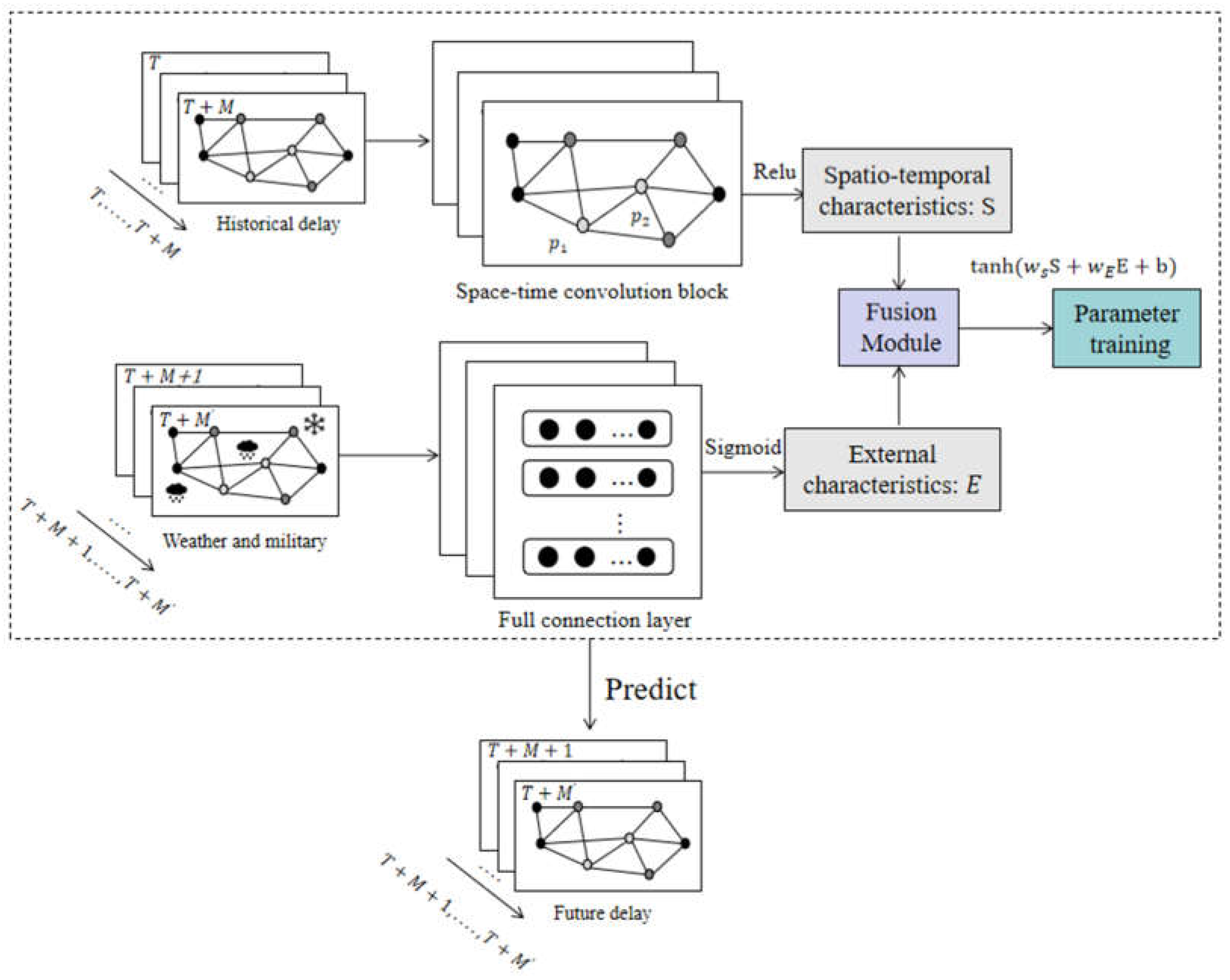
Appendix B.2. Spatiotemporal Convolution Module

The spatiotemporal feature extraction module first employs spectral graph convolution (SGC) to capture spatial dependencies. To address the irregular topology and complex node interactions in airport networks, we define the graph Laplacian matrix:

$$L=D-W$$

(A5)

where D is the degree matrix, and W is the weight matrix.

Through eigendecomposition, graph signals are transformed into the spectral domain via graph Fourier transform for convolution operations. To mitigate computational complexity in large-scale networks, Chebyshev polynomial approximation is adopted. By adjusting the polynomial order, the model extracts spatial delay propagation patterns within the airport network.

The temporal gated convolutional layer uses one-dimensional causal convolution to process historical delay sequences. Key temporal information is dynamically filtered through a gated linear unit (GLU) to suppress noise and enhance feature representation. Residual connections are added to the convolutional layers to alleviate the gradient vanishing problem caused by increased network depth. Multiple temporally gated convolutional layers are stacked to extract multi-scale temporal features.

The time-gated convolution layer and spatial spectral convolution layer then form a spatiotemporal convolution block, which acts on the time-series data generated by each node of the airport network. Subsequently, an activation function is used to increase the nonlinear relationship between the convolution layers. Finally, a time convolution layer is added to reduce the dimensions of the extracted multidimensional features.

Appendix B.3. External Feature Extraction Module

Poor weather conditions and military activities can significantly affect flight delays. To address these external disturbances, an external feature extraction module is integrated to refine the prediction. Specifically, meteorological data (wind speed, visibility, and precipitation) and military activity indicators are encoded as input features. A fully connected layer is first applied to reduce the feature dimensions and extract critical patterns. Subsequently, a temporal convolution layer convolves the processed features to generate a one-step prediction. Additionally, layer normalization is applied to the output to prevent overfitting.

Appendix B.4. Fusion Module

We then use a linear transformation to integrate the output data of the above two modules. Moreover, we map the multidimensional features of the output to one dimension and transform the output value to [−1,1] using the activation function tanh.

Appendix B.5. Model Validation

To comparatively validate the predictive performance of the model, the proposed STGCN method in this paper is compared with three traditional time series forecasting approaches: the historical mean method (where the predicted value is the average of airport flight delay times over a specific historical period), random forest [50], and LSTM networks [51]. The baseline models are appropriately constructed based on relevant literature. Each model utilizes historical delay data to predict future average airport departure delay times. For ease of comparison, the prediction time windows are set to 1 h and 4 h. We select Test Case (1) to Test Case (6) from Section 5.2 for model training and prediction. The mean absolute error (MAE) is adopted to evaluate the prediction results of each algorithm.

The spatiotemporal feature extraction module in the model consists of two stacked spatiotemporal convolutional blocks with channel numbers of 32 and 64, respectively. The kernel sizes of both the spatial convolutional layer and the temporal gated convolutional layer are set to 3. The initial learning rate is 0.01, decaying by 70% every 10 epochs, with a maximum iteration count of 50 and a batch size of 100. The prediction performances of all models are summarized in Table A1.

Table A1. Predictive accuracy: STGCN vs. baseline models.

Data Set	Evaluation Metric	Time Window (h)	Historical Mean Method	Random Forest	LSTM Networks	STGCN
Test Case (1)	MAE	1	6.124	4.357	4.212	3.852
		4	6.124	4.525	4.473	4.021
Test Case (2)	MAE	1	5.965	4.124	4.027	3.783
		4	5.965	4.253	4.224	3.971
Test Case (3)	MAE	1	5.373	3.642	3.526	3.374
		4	5.373	3.733	3.664	3.625
Test Case (4)	MAE	1	5.594	4.012	3.857	3.656
		4	5.594	4.276	4.018	3.829
Test Case (5)	MAE	1	5.923	4.124	4.002	3.798
		4	5.923	4.398	4.215	3.865
Test Case (6)	MAE	1	5.235	3.685	3.593	3.312
		4	5.235	3.741	3.737	3.542

Table A1. Predictive accuracy: STGCN vs. baseline models.

Data Set	Evaluation Metric	Time Window (h)	Historical Mean Method	Random Forest	LSTM Networks	STGCN
Test Case (1)	MAE	1	6.124	4.357	4.212	3.852
		4	6.124	4.525	4.473	4.021
Test Case (2)	MAE	1	5.965	4.124	4.027	3.783
		4	5.965	4.253	4.224	3.971
Test Case (3)	MAE	1	5.373	3.642	3.526	3.374
		4	5.373	3.733	3.664	3.625
Test Case (4)	MAE	1	5.594	4.012	3.857	3.656
		4	5.594	4.276	4.018	3.829
Test Case (5)	MAE	1	5.923	4.124	4.002	3.798
		4	5.923	4.398	4.215	3.865
Test Case (6)	MAE	1	5.235	3.685	3.593	3.312
		4	5.235	3.741	3.737	3.542

As shown in Table A1, the STGCN model achieves superior performance across most scenarios in terms of the MAE compared to other baseline models under most scenarios, while the historical mean method demonstrates the weakest performance among all baseline models. Deep learning-based approaches exhibit significantly better predictive capabilities than the random forest method, further confirming that deep learning algorithms can effectively uncover latent patterns from nonlinear and complex datasets.

To further validate the impact of severe weather and military activity features on prediction accuracy, we construct a variant model STGCN-N by removing the external feature extraction module from STGCN. The corresponding prediction performance is presented in Table A2.

Table A2. Predictive accuracy: STGCN vs. STGCN-N.

Data Set	Time Window (h)	MAE (min)		% R
		STGCN	STGCN-N
Test Case (1)	1	3.852	4.201	57.0
	4	4.021	4.503	56.6
Test Case (2)	1	3.783	4.021	55.1
	4	3.971	4.233	54.7
Test Case (3)	1	3.374	3.502	43.0
	4	3.425	3.679	42.5
Test Case (4)	1	3.656	3.861	45.6
	4	3.829	4.052	47.2
Test Case (5)	1	3.798	4.019	50.4
	4	3.865	4.189	52.6
Test Case (6)	1	3.312	3.615	42.1
	4	3.542	3.859	41.9

Table A2. Predictive accuracy: STGCN vs. STGCN-N.

Data Set	Time Window (h)	MAE (min)		% R
		STGCN	STGCN-N
Test Case (1)	1	3.852	4.201	57.0
	4	4.021	4.503	56.6
Test Case (2)	1	3.783	4.021	55.1
	4	3.971	4.233	54.7
Test Case (3)	1	3.374	3.502	43.0
	4	3.425	3.679	42.5
Test Case (4)	1	3.656	3.861	45.6
	4	3.829	4.052	47.2
Test Case (5)	1	3.798	4.019	50.4
	4	3.865	4.189	52.6
Test Case (6)	1	3.312	3.615	42.1
	4	3.542	3.859	41.9

Define $R$ as the proportion of nodes where the MAE between the STGCN model’s predicted airport delay times and the ground-truth values on a given test set is lower than that of the STGCN-N model across all prediction nodes. As shown in Table A2, the $R$ values exceed 40% in all datasets, validating that the external factor features (weather and military activity) served a corrective role in refining the prediction results.

Appendix C.1. Aircraft-Routing Constraints

Flight-connection constraints: By guaranteeing that each flight has one predecessor and one successor in rotation, Constraints (A6) and (A7) ensure the connectivity of the aircraft connection network. Meanwhile, the first flight has a pre-sequence dummy flight, and the last flight has a post-sequence dummy flight.

$$\sum _{i:(i,j)\in A^k\cup A_D^k}{x}_{ij}=1, \forall f\in F,k\in K^f,j\in L^k,$$

(A6)

$$\sum _{i:(j,i)\in A^k\cup A_A^k}{x}_{ji}=1, \forall f\in F,k\in K^f,j\in L^k,$$

(A7)

Aircraft-capacity constraints: Constraint (A8) requires that the total number of aircraft in service for aircraft rotation should not exceed the available number by limiting the number of starting arcs.

$$\sum _{(i,j)\in A_D^k}{x}_{ij}\le N^k,\forall f\in F,k\in K^f,$$

(A8)

Flow-conservation constraints: Constraint (A9) guarantees the flow conservation of the aircraft in each rotation by balancing the dummy starting and ending arcs.

$$\sum _{(i,j)\in A_{A_p}^k}{x}_{ij}-\sum _{(i,j)\in A_{D_p}^k}{x}_{ij}=0,\forall f\in F,k\in K^f,p\in P,$$

(A9)

Maintenance-feasibility constraints: Nonlinear Constraints (A10)–(A19) ensure aircraft maintenance feasibility. More precisely, Constraints (A10)–(A12) restrict the total flying time of the aircraft. Constraints (A13)–(A15) ensure that the maximum takeoff and landing restrictions are satisfied. Constraints (A16)–(A19) ensure a maximum calendar day restriction for the aircraft.

$$u_j^a{x}_{ij}=t_j{x}_{ij},\forall f\in F,k\in K^f,j\in L^k,(i,j)\in A_M^k,$$

(A10)

$$u_j^a{x}_{ij}=(u_i^a+t_j)x_{ij},\forall f\in F,k\in K^f,j\in L^k,(i,j)\in A_{NM}^k,$$

(A11)

$$t_j\le u_j^a\le t_{max}^k,\forall f\in F,k\in K^f,j\in L^k,$$

(A12)

$${\mu }_j^a{x}_{ij}=x_{ij},\forall f\in F,k\in K^f,j\in L^k,(i,j)\in A_M^k,$$

(A13)

$${\mu }_j^a{x}_{ij}=({\mu }_j^a+1)x_{ij},\forall f\in F,k\in K^f,j\in L^k,(i,j)\in A_{NM}^k,$$

(A14)

$$1\le {\mu }_j^a\le {\mu }_{max}^k,\forall f\in F,k\in K^f,j\in L^k,$$

(A15)

$$d_j{x}_{ij}=x_{ij},\forall f\in F,k\in K^f,j\in L^k,(i,j)\in A_M^k,$$

(A16)

$$d_j{x}_{ij}=d_i{x}_{ij},\forall f\in F,k\in K^f,j\in L^k,(i,j)\in A_3^k,$$

(A17)

$$d_j{x}_{ij}=(d_i+1)x_{ij},\forall f\in F,k\in K^f,j\in L^k,(i,j)\in A_4^k,$$

(A18)

$$t_j\le d_j\le d_{max}^k,\forall f\in F,k\in K^f,j\in L^k,$$

(A19)

Appendix C.2. Crew-Pairing Constraints

Flight-connection constraints: Constraints (A20) and (A21) ensure the connectivity of the crew connection network by ensuring that each flight has one predecessor and one successor for each pairing. Additionally, a starting/ending flight has a pre-sequence/post-sequence dummy flight.

$$\sum _{i:(i,j)\in B^f\cup B_D^f}{y}_{ij}=1,\forall f\in F,j\in L^f,$$

(A20)

$$\sum _{i:(j,i)\in B^f\cup B_A^f}{y}_{ji}=1,\forall f\in F,j\in L^f,$$

(A21)

Crew-capacity constraints: Constraint (A22) is imposed to ensure that the total number of crew members for the considered aircraft family does not exceed the qualified capacity.

$$\sum _{(i,j)\in B_D^f}{y}_{ij}\le N^f,\forall f\in F,j\in L^f,$$

(A22)

Flow-conservation constraints: Constraint (A23) guarantees flow conservation for the crew.

$$\sum _{(i,j)\in B_{D_p}^f}{y}_{ij}-\sum _{(i,j)\in B_{A_p}^f}{y}_{ij}=0,\forall f\in F,p\in P,$$

(A23)

Duty and pairing feasibility constraints: Quadratic Constraints (A24)–(A41) ensure the feasibility of pairing and duty. Specifically, Constraints (A24)–(A26) help tally the total flying time and impose restrictions accordingly. Constraints (A27)–(A29) limit the maximum takeoff and landing times for the crew in one duty. Constraints (A30)–(A32) ensure that the duty duration does not exceed the maximum restricted value. Constraints (A33)–(A36) require that the number of duties within a pairing does not exceed the designated restriction. Constraints (A37)–(A41) ensure that the maximum time away from the base is adhered to.

$$u_j^c{y}_{ij}=t_j{y}_{ij},\forall f\in F,j\in L^f,(i,j)\in B_2^f\cup B_D^f,$$

(A24)

$$u_j^c{y}_{ij}=(u_i^c+t_j)y_{ij},\forall f\in F,j\in L^f,(i,j)\in B_1^f,$$

(A25)

$$1\le u_j^c\le t_{max}^c,\forall f\in F,j\in L^f,$$

(A26)

$${\mu }_j^c{y}_{ij}=y_{ij},\forall f\in F,j\in L^f,(i,j)\in B_2^f\cup B_D^f,$$

(A27)

$${\mu }_j^c{y}_{ij}=({\mu }_i^c+1)y_{ij},\forall f\in F,j\in L^f,(i,j)\in B_1^f,$$

(A28)

$$1\le {\mu }_j^c\le {\mu }_{max}^c,\forall f\in F,j\in L^f,$$

(A29)

$${\lambda }_j{y}_{ij}=t_j{y}_{ij},\forall f\in F,j\in L^f,(i,j)\in B_2^f\cup B_D^f,$$

(A30)

$${\lambda }_j{y}_{ij}=({\lambda }_i+s_{ij}+t_j)y_{ij},\forall f\in F,j\in L^f,(i,j)\in B_1^f,$$

(A31)

$$t_j\le {\lambda }_j\le {\lambda }_{max},\forall f\in F,j\in L^f,$$

(A32)

$$v_j{y}_{ij}=y_{ij},\forall f\in F,j\in L_D^f,(i,j)\in B_D^f,$$

(A33)

$$v_j{y}_{ij}=v_i{y}_{ij},\forall f\in F,j\in L^f,(i,j)\in B_1^f,$$

(A34)

$$v_j{y}_{ij}=(v_i+1)y_{ij},\forall f\in F,j\in L^f,(i,j)\in B_2^f,$$

(A35)

$$1\le v_j\le v_{max},\forall f\in F,j\in L^f,$$

(A36)

$${\eta }_j{y}_{ij}=t_j{y}_{ij},\forall f\in F,j\in L_D^f,(i,j)\in B_D^f,$$

(A37)

$${\eta }_j{y}_{ij}=({\eta }_i+s_{ij}+t_j)y_{ij},\forall f\in F,j\in L^f,(i,j)\in B_1^f,$$

(A38)

$${\eta }_j{y}_{ij}=({\eta }_i+l_{ij}+t_j)y_{ij},\forall f\in F,j\in L^f,(i,j)\in B_2^f,$$

(A39)

$${\eta }_i\ge {\eta }_{min}{y}_{ij},\forall f\in F,j\in L_A^f,(i,j)\in B_A^f,$$

(A40)

$$t_j\le {\eta }_j\le {\eta }_{min},\forall f\in F,j\in L^f,$$

(A41)

Appendix C.3. Linking Constraints

Short-connection constraints: Constraint (A42) ensures that the crew must follow the aircraft in the short connection; otherwise, the short connection should not be selected.

$$y_{ij}\le x_{ij},\forall f\in F,(i,j)\in B_s^f,$$

(A42)

Relationship between $x,y, \mathrm{a}\mathrm{n}\mathrm{d} z$: Constraints (A43)–(A46) guarantee that $z_{ij}=1$ if and only if $x_{ij}$ and $y_{ij}$ are both equal to 1.

$$0\le z_{ij}\le x_{ij},\forall f\in F,(i,j)\in A^k\cap B^f,\forall k\in K^f,j\in L^k,$$

(A43)

$$0\le z_{ij}\le y_{ij},\forall f\in F,(i,j)\in A^k\cap B^f,\forall k\in K^f,j\in L^k,$$

(A44)

$$z_{ij}\ge x_{ij}+y_{ij}-1,\forall f\in F,(i,j)\in A^k\cap B^f,\forall k\in K^f,j\in L^k,$$

(A45)

$$x_{ij}, y_{ij}, z_{ij}\in \left\{\mathrm{0,1}\right\},\forall i,j\in L.$$

(A46)

References

1. Xu, Y.; Wandelt, S.; Sun, X. Airline integrated robust scheduling with a variable neighborhood search based heuristic. Transp. Res. Part B Methodol. 2021, 149, 181–203. [Google Scholar] [CrossRef]
2. Birolini, S.; Antunes, A.P.; Cattaneo, M.; Malighetti, P.; Paleari, S. Integrated flight scheduling and fleet assignment with improved supply-demand interactions. Transp. Res. Part B Methodol. 2021, 149, 162–180. [Google Scholar] [CrossRef]
3. Yan, C.; Barnhart, C.; Vaze, V. Choice-based airline schedule design and fleet assignment: A decomposition approach. Transp. Sci. 2022, 56, 1410–1431. [Google Scholar] [CrossRef]
4. Kızıloğlu, K.; Sakallı, Ü.S. Integrating Flight Scheduling, Fleet Assignment, and Aircraft Routing Problems with Codesharing Agreements under Stochastic Environment. Aerospace 2023, 10, 1031. [Google Scholar] [CrossRef]
5. Ding, C.; Guo, Y.; Weng, J. Robust Model for Fleet Assignment with Station Purity and Robust Opportunities. In Proceedings of the 2021 9th International Conference on Information Technology: IoT and Smart City, Guangzhou, China, 22–25 December 2021. [Google Scholar]
6. Liu, M.; Ding, Y.; Sun, L.; Zhang, R.; Dong, Y.; Zhao, Z.; Wang, Y.; Liu, C. Green Airline-Fleet Assignment with Uncertain Passenger Demand and Fuel Price. Sustainability 2023, 15, 899. [Google Scholar] [CrossRef]
7. Khanmirza, E.; Nazarahari, M.; Haghbeigi, M. A heuristic approach for optimal integrated airline schedule design and fleet assignment with demand recapture. Appl. Soft Comput. 2020, 96, 106681. [Google Scholar] [CrossRef]
8. Eltoukhy, A.E.; Chan, F.T.; Chung, S.H.; Niu, B.; Wang, X.P. Heuristic approaches for operational aircraft maintenance routing problem with maximum flying hours and man-power availability considerations. Ind. Manag. Data Syst. 2017, 117, 2142–2170. [Google Scholar] [CrossRef]
9. Eltoukhy, A.E.; Wang, Z.X.; Chan, F.T.; Chung, S.H.; Ma, H.L.; Wang, X.P. Robust aircraft maintenance routing problem using a turn-around time reduction approach. IEEE Trans. Syst. Man Cybern. Syst. 2019, 50, 4919–4932. [Google Scholar] [CrossRef]
10. Birolini, S.; Jacquillat, A. Day-ahead aircraft routing with data-driven primary delay predictions. Eur. J. Oper. Res. 2023, 310, 379–396. [Google Scholar] [CrossRef]
11. Akıncılar, A.; Güner, E. A new tool for robust aircraft routing: Superior Robust Aircraft Routing (sup-RAR). J. Air Transp. Manag. 2025, 124, 102744. [Google Scholar] [CrossRef]
12. Wen, X.; Chung, S.H.; Choi, T.M.; Fu, X. Airline cabin crew pairing with accurate characterization of cross-class substitution: A branch-and-price approach. Transp. Res. Part B Methodol. 2024, 190, 103084. [Google Scholar] [CrossRef]
13. Ding, C.; Chen, X.; Wu, W.; Wei, W.; Xin, Z. Game-theoretic analysis of the impact of crew overnight hotel cost on airlines’ fleet assignment and crew pairing. J. Air Transp. Manag. 2023, 113, 102491. [Google Scholar] [CrossRef]
14. Zeren, B.; Özcan, E.; Deveci, M. An adaptive greedy heuristic for large scale airline crew pairing problems. J. Air Transp. Manag. 2024, 114, 102492. [Google Scholar] [CrossRef]
15. Cacchiani, V.; Salazar-González, J.J. Optimal solutions to a real-world integrated airline scheduling problem. Transp. Sci. 2017, 51, 250–268. [Google Scholar] [CrossRef]
16. Shao, S.; Sherali, H.D.; Haouari, M. A novel model and decomposition approach for the integrated airline fleet assignment, aircraft routing, and crew pairing problem. Transp. Sci. 2017, 51, 233–249. [Google Scholar] [CrossRef]
17. Ahmed, M.B.; Hryhoryeva, M.; Hvattum, L.M.; Haouari, M. A matheuristic for the robust integrated airline fleet assignment, aircraft routing, and crew pairing problem. Comput. Oper. Res. 2023, 137, 105551. [Google Scholar] [CrossRef]
18. Mercier, A.; Cordeau, J.F.; Soumis, F. A computational study of Benders decomposition for the integrated aircraft routing and crew scheduling problem. Comput. Oper. Res. 2005, 32, 1451–1476. [Google Scholar] [CrossRef]
19. Yan, C.; Kung, J. Robust aircraft routing. Transp. Sci. 2018, 52, 118–133. [Google Scholar] [CrossRef]
20. Ma, H.L.; Sun, Y.; Chung, S.H.; Chan, H.K. Tackling uncertainties in aircraft maintenance routing: A review of emerging technologies. Transp. Res. Part E Logist. Transp. Rev. 2022, 164, 102805. [Google Scholar] [CrossRef]
21. Wen, X.; Ma, H.L.; Chung, S.H.; Khan, W.A. Robust airline crew scheduling with flight flying time variability. Transp. Res. Part E Logist. Transp. Rev. 2020, 144, 102132. [Google Scholar] [CrossRef]
22. Cordeau, J.F.; Stojković, G.; Soumis, F.; Desrosiers, J. Benders decomposition for simultaneous aircraft routing and crew scheduling. Transp. Sci. 2001, 35, 375–388. [Google Scholar] [CrossRef]
23. Weide, O.; Ryan, D.; Ehrgott, M. An iterative approach to robust and integrated aircraft routing and crew scheduling. Comput. Oper. Res. 2010, 37, 833–844. [Google Scholar] [CrossRef]
24. Ruther, S.; Boland, N.; Engineer, F.G.; Evans, I. Integrated aircraft routing, crew pairing, and tail assignment: Branch-and-price with many pricing problems. Transp. Sci. 2017, 51, 177–195. [Google Scholar] [CrossRef]
25. Ahmed, M.B.; Mansour, F.Z.; Haouari, M. Robust integrated maintenance aircraft routing and crew pairing. J. Air Transp. Manag. 2018, 73, 15–31. [Google Scholar] [CrossRef]
26. Dunbar, M.; Froyland, G.; Wu, C.L. Robust airline schedule planning: Minimizing propagated delay in an integrated routing and crewing framework. Transp. Sci. 2012, 46, 204–216. [Google Scholar] [CrossRef]
27. Dunbar, M.; Froyland, G.; Wu, C.L. An integrated scenario-based approach for robust aircraft routing, crew pairing and re-timing. Comput. Oper. Res. 2014, 45, 68–86. [Google Scholar] [CrossRef]
28. Cacchiani, V.; Salazar-González, J.J. Heuristic approaches for flight retiming in an integrated airline scheduling problem of a regional carrier. Omega 2020, 91, 102028. [Google Scholar] [CrossRef]
29. Dück, V.; Ionescu, L.; Kliewer, N.; Suhl, L. Increasing stability of crew and aircraft schedules. Transp. Res. Part C Emerg. Technol. 2012, 20, 47–61. [Google Scholar] [CrossRef]
30. Ruan, J.H.; Wang, Z.X.; Chan, F.T.; Patnaik, S.; Tiwari, M.K. A reinforcement learning-based algorithm for the aircraft maintenance routing problem. Expert Syst. Appl. 2021, 169, 114399. [Google Scholar] [CrossRef]
31. Hu, Y.; Miao, X.; Zhang, J.; Liu, J.; Pan, E. Reinforcement learning-driven maintenance strategy: A novel solution for long-term aircraft maintenance decision optimization. Comput. Ind. Eng. 2021, 153, 107056. [Google Scholar] [CrossRef]
32. Li, Y.; Wang, X.; Kang, Q.; Fan, Z.; Yao, S. An MCTS-Based Solution Approach to Solve Large-Scale Airline Crew Pairing Problems. IEEE Trans. Intell. Transp. Syst. 2023, 24, 5477–5488. [Google Scholar] [CrossRef]
33. Thakkar, D.; Palaniappan, B. Aircraft routing using dynamic programming and reinforcement learning: A customer-centric approach. J. Air Transp. Res. Soc. 2024, 2, 100018. [Google Scholar] [CrossRef]
34. Yuan, J.; Pei, Y.; Xu, Y.; Ge, Y.; Wei, Z. Autonomous interval management of multi-aircraft based on multi-agent reinforcement learning considering fuel consumption. Transp. Res. Part C Emerg. Technol. 2024, 165, 104729. [Google Scholar] [CrossRef]
35. Lee, J.; Lee, K.; Moon, I. A reinforcement learning approach for multi-fleet aircraft recovery under airline disruption. Appl. Soft Comput. 2022, 129, 109556. [Google Scholar] [CrossRef]
36. Li, H.; Wu, X.; Ribeiro, M.; Santos, B.; Zheng, P. Deep reinforcement learning approach for real-time airport gate assignment. Oper. Res. Perspect. 2025, 14, 100338. [Google Scholar] [CrossRef]
37. Eltoukhy, A.E.; Wang, Z.X.; Shaban, I.A.; Chan, F.T. Coordinating aircraft maintenance routing and integrated maintenance staffing and rostering: A Stackelberg game theoretical model. Int. J. Prod. Res. 2022, 60, 7450–7474. [Google Scholar] [CrossRef]
38. Haouari, M.; Shao, S.; Sherali, H.D. A lifted compact formulation for the daily aircraft maintenance routing problem. Transp. Sci. 2013, 47, 508–525. [Google Scholar] [CrossRef]
39. Sanchez, D.T.; Boyacı, B.; Zografos, K.G. An optimisation framework for airline fleet maintenance scheduling with tail assignment considerations. Transp. Res. Part B Methodol. 2020, 133, 142–164. [Google Scholar] [CrossRef]
40. Haouari, M.; Zeghal Mansour, F.; Sherali, H.D. A new compact formulation for the daily crew pairing problem. Transp. Sci. 2019, 53, 811–828. [Google Scholar] [CrossRef]
41. AhmadBeygi, S.; Cohn, A.; Guan, Y.; Belobaba, P. Analysis of the potential for delay propagation in passenger airline networks. J. Air Transp. Manag. 2008, 14, 221–236. [Google Scholar] [CrossRef]
42. GiGiannikas, V.; Ledwoch, A.; Stojković, G.; Costas, P.; Brintrup, A.; Al-Ali, A.A.S.; Chauhan, V.K.; McFarlane, D. A data-driven method to assess the causes and impact of delay propagation in air transportation systems. Transp. Res. Part C Emerg. Technol. 2022, 143, 103862. [Google Scholar] [CrossRef]
43. Dück, V. Increasing Stability of Aircraft and Crew Schedules. Ph.D. Thesis, Paderborn University, Paderborn, Germany, 2010. [Google Scholar]
44. Moerland, T.M.; Broekens, J.; Plaat, A.; Jonker, C.M. Model-based reinforcement learning: A survey. Found. Trends Mach. Learn. 2023, 16, 1–118. [Google Scholar] [CrossRef]
45. Szepesvári, C. Algorithms for Reinforcement Learning; Springer Nature: Berlin/Heidelberg, Germany, 2022. [Google Scholar]
46. Liu, Y.; Chen, Y.; Jiang, T. Dynamic selective maintenance optimization for multi-state systems over a finite horizon: A deep reinforcement learning approach. Eur. J. Oper. Res. 2020, 283, 166–181. [Google Scholar] [CrossRef]
47. Bennett, A.; Kallus, N. Proximal reinforcement learning: Efficient off-policy evaluation in partially observed markov decision processes. Oper. Res. 2023, 72, 1071–1086. [Google Scholar] [CrossRef]
48. Lee, H.R.; Lee, T. Multi-agent reinforcement learning algorithm to solve a partially-observable multi-agent problem in disaster response. Eur. J. Oper. Res. 2021, 291, 296–308. [Google Scholar] [CrossRef]
49. Aloulou, M.A.; Haouari, M.; Mansour, F.Z. A model for enhancing robustness of aircraft and passenger connections. Transp. Res. Part C Emerg. Technol. 2013, 32, 48–60. [Google Scholar] [CrossRef]
50. Rebollo, J.J.; Balakrishnan, H. Characterization and prediction of air traffic delays. Transp. Res. Part C Emerg. Technol. 2014, 44, 231–241. [Google Scholar] [CrossRef]
51. Gui, G.; Liu, F.; Sun, J.; Yang, J.; Zhou, Z.; Zhao, D. Flight delay prediction based on aviation big data and machine learning. IEEE Trans. Veh. Technol. 2019, 69, 140–150. [Google Scholar] [CrossRef]