Relative Pose Estimation of an Uncooperative Target with Camera Marker Detection

Abstract

Accurate and robust relative pose estimation is the first step in ensuring the success of an active debris removal mission. This paper introduces a novel method to detect structural markers on the European Space Agency’s Environmental Satellite (ENVISAT) for safe de-orbiting using image processing and Convolutional Neural Networks (CNNs). Advanced image preprocessing techniques, including noise addition and blurring, are employed to improve marker detection accuracy and robustness from a chaser spacecraft. Additionally, we address the challenges posed by eclipse periods, during which the satellite’s corners are not visible, preventing measurement updates in the Unscented Kalman Filter (UKF). To maintain estimation quality in these periods of data loss, we propose a covariance-inflating approach in which the process noise covariance matrix is adjusted, reflecting the increased uncertainty in state predictions during the eclipse. This adaptation ensures more accurate state estimation and system stability in the absence of measurements. The initial results show promising potential for autonomous removal of space debris, supporting proactive strategies for space sustainability. The effectiveness of our approach suggests that our estimation method, combined with robust noise adaptation, could significantly enhance the safety and efficiency of debris removal operations by implementing more resilient and autonomous systems in actual space missions.

1. Introduction

The escalating problem of space debris necessitates innovative solutions for identification and removal with a high level of autonomy [1], particularly for large defunct satellites such as ESA’s ENVISAT, an inactive Earth observation satellite. In the past ten years, deep learning (DL) has profoundly influenced the development of computer vision algorithms, enhancing their performance and robustness in various applications such as image classification, segmentation, and object tracking. This momentum has carried into spacecraft pose estimation, where DL-based methods have begun to surpass traditional feature-engineering techniques reported in the literature [2,3], corner and marker detection algorithms such as FAST, Shi-Tomasi, and Hough transform methods [4,5,6,7]. CNNs have shown promising results in spacecraft pose estimation tasks, particularly for non-cooperative targets. Previous studies have utilized a variety of techniques, including perspective-n-point (PnP) algorithms [8], blob detection methods [9], and region-based methods [10,11], to estimate spacecraft poses from monocular images. These methods, while effective under controlled conditions, often struggle with challenges such as poor lighting, sensor noise, and complex geometries typical of space-based imagery [12]. Generally, the scarcity of extensive synthetic space image datasets, crucial for comprehensive CNN training, necessitates the use of networks pre-trained on terrestrial images. To adapt these for space applications, transfer learning is used, focusing on training only selected layers of the CNN [13]. Detection of key points such as corners involves predicting the 2D projections of specific 3D key points from the spacecraft’s imaged segments using a deep learning model. These key points are usually determined by the CAD model of the spacecraft. In the absence of a CAD model, methods like multi-view triangulation or structure from motion are employed to create a 3D wire frame model that includes these key points [14,15]. The key point location regression technique involves direct estimation of key point positions [16,17]. The segmentation-driven method utilizes a network with dual functions, segmentation and regression, to deduce key point locations. The image is sectioned into a grid, isolating the spacecraft within certain grid cells. The positions of the key points are then computed as offsets within these identified cells, which improves the prediction accuracy. Variations of this model have been optimized for space deployment, reducing the parameter count without compromising the accuracy of prediction [18,19]. The heat map prediction method represents the likelihood of key point locations from which the highest probability points are extracted as the actual locations. Moreover, there is a bounding box approach using the enclosed bounding boxes over the key points that are predicted along with confidence scores rather than using the key point locations or heat maps [20,21]. Recent work [22] has highlighted the limitations of feature-based approaches and demonstrated how CNNs can overcome some of these challenges, improving robustness against sensor noise and environmental variations. In this study, we expand on these efforts by leveraging CNNs to detect structural markers on the ENVISAT satellite, which is crucial for autonomous space debris removal and de-orbiting operations.

On the other hand, the estimation algorithms are an integral part of determining the spacecraft pose, and they involve deducing the value of a desired quantity from indirect, imprecise, and noisy observations. When this quantity is the current state of a dynamic system, the process is termed as the best estimate obtained from the measurements. Moreover, estimation of the relative position and the target attitude are crucial for safe proximity operations. This necessitates complex on-board computations at a frequency ensuring accuracy requirements are met. However, the limited computational power of current processors constrains the estimation processes. Therefore, developing efficient algorithms that minimize computational demands while maintaining necessary performance and reaching the best estimate are crucial for the sake of these missions. This estimate is produced by an optimal estimator, a computational algorithm, effectively utilizing available data, system knowledge, and disturbance information. For linear and Gaussian scenarios, the posterior distribution remains Gaussian, and the Kalman Filter (KF) is used to compute its mean and covariance matrix. However, practical problems are often nonlinear, leading to non-Gaussian probability density functions (PDFs). Various techniques address non-linear estimation problems in space applications. One straightforward method is to linearize the dynamics and measurement equations around the current estimate, as done in the Extended Kalman Filter (EKF) [23], which applies KF mechanics to a linearized system. Higher-order Taylor series approximations can extend the EKF’s first-order approximation. The Gaussian Second-Order Filter (GSOF), for example, truncates the Taylor series at the second order to better handle system nonlinearity [24]. This requires knowledge of the estimation error’s central moments up to the fourth order to calculate the Kalman gain. For instance, while the EKF uses first-order truncation requiring covariance matrices, the GSOF requires third and fourth central moments of the state distribution. The GSOF approximates the prior PDF as Gaussian at each iteration and performs a linear update based on a second-order approximation of the posterior estimation error. Other linear filters use different approximations, such as Gaussian quadrature, spherical cubature, ensemble points, central differences, and finite differences [25]. Alternatively, the Unscented Kalman Filter (UKF) employs the unscented transformation to better manage nonlinearity in dynamics and measurements, typically achieving higher accuracy and robustness than the EKF. The UKF uses this transformation for a more precise approximation of the predicted mean and covariance matrix, remaining a linear estimator where the estimate is a linear function of the current measurement [26]. The UKF offers a solution by using the unscented transformation, which avoids linearization by propagating carefully selected sample points through the nonlinear system, providing superior performance in such situations [27,28]. Recently, even the use of artificial intelligence methods for non-linear estimation has also been reported in the literature [29,30].

In this paper, we address a novel approach using image processing from a chaser spacecraft to detect structural markers on the ENVISAT satellite, as well as an estimation framework utilizing UKF to facilitate its safe de-orbiting. Utilizing high-resolution imagery, this study employs our own CNN, TinyCornerNET, designed for precise marker detection, essential for the subsequent removal process. The methodology incorporates image preprocessing, including noise addition, to enhance feature detection accuracy under varying space conditions. Each image taken by the camera is processed via the CNN, which provides corner measurements to the filter, and the filter predicts the required relative pose states. This is challenging due to the tumbling motion of ENVISAT. Until this point, there is no merged solution for this problem; therefore, we propose a full pipeline for the relative pose navigation system, where the relative position and velocity states are estimated for both translational and angular components. To enhance the robustness and to propose a realistic scenario, this work introduces a tuning process for noise covariance matrix ($\mathbf{Q}$) adjustment during eclipse periods, when the satellite’s corner markers become occluded and measurements are unavailable, which was not studied in recent works [31]. This approach ensures that the state estimation remains robust by accounting for increased uncertainty during these periods of no visibility, thus improving the accuracy of both translational and rotational state predictions. By adjusting $\mathbf{Q}$ during eclipse periods, the UKF can effectively mitigate the risk of estimation divergence, maintaining system stability and ensuring accurate tracking even in the absence of real-time measurements. Preliminary results demonstrate the system’s efficacy in identifying corner points on the satellite and its ability to maintain translational and rotational estimates within appropriate levels, promising a significant leap forward in automated space debris removal technologies. This work builds on recent advances in space debris monitoring and removal strategies, echoing the urgent call for action highlighted in studies such as [32,33,34], which emphasize the growing threat of space debris and the need for effective removal mechanisms [35]. Our findings indicate a scalable solution for debris management, aligned with the proactive strategies recommended by the Inter-Agency Space Debris Coordination Committee (IADC) [36].

2. Methodology

In this section, the methodology underlying the proposed approach is detailed. It covers the dynamics governing both the chaser and the target spacecraft, the simulation setup for the ENVISAT satellite, and the process of preparing the data for image-based measurements and estimation.

2.1. Dynamics

In the following analysis, several assumptions are made to represent the dynamics modeling the chaser and target spacecraft. Firstly, it is presumed that the inertia properties of both the chaser and the target are perfectly known beforehand. This assumption simplifies the dynamic modeling by removing uncertainties related to mass distribution and moments of inertia. Secondly, the absolute motion of the chaser is considered deterministic. Lastly, neither flexible dynamics nor external disturbances are taken into account. This implies that the translational and rotational dynamics are decoupled. These assumptions streamline the analysis by focusing on the primary dynamics without uncertain factors. However, they are validated by the knowledge of the scenario, as ENVISAT’s models are known and available to the public. Therefore, the motion of the chaser and the target can be represented as follows.

2.1.1. Absolute Chaser Motion

The chaser motion is described by the following equations, where $\mu$ is the gravitational parameter of the Earth, $\overline{r}$ is the position of the chaser center of mass with respect to the Earth, and $\theta$ is the true anomaly in the orbit of the chaser.

$$\begin{array}{c}\hfill \ddot{\overline{r}}=\overline{r}{\dot{\theta }}^2-{\displaystyle \frac{\mu }{{\overline{r}}^2}}\end{array}$$

(1)

$$\begin{array}{c}\hfill \ddot{\theta }=-2{\displaystyle \frac{\dot{\overline{r}}\dot{\theta }}{\overline{r}}}\end{array}$$

(2)

2.1.2. Relative Translational Dynamics

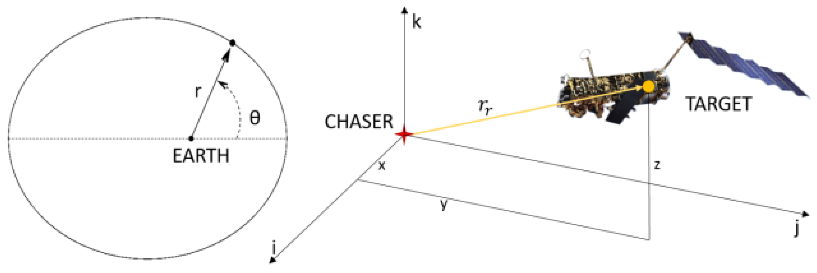
The target, ENVISAT, has its relative translational dynamic equations developed with respect to the local-vertical–local-horizontal (LVLH) frame of the chaser. The target relative position, denoted as ${\mathbf{r}}_{\mathbf{r}}$, and relative velocity, ${\mathbf{v}}_{\mathbf{r}}$, are defined in the chaser LVLH frame, expressed as follows:

$$\begin{array}{cc}\hfill {\mathbf{r}}_{\mathbf{r}}& =x\widehat{\mathbf{i}}+y\widehat{\mathbf{j}}+z\widehat{\mathbf{k}}\hfill \end{array}$$

(3)

$$\begin{array}{cc}\hfill {\mathbf{v}}_{\mathbf{r}}& =\dot{x}\widehat{\mathbf{i}}+\dot{y}\widehat{\mathbf{j}}+\dot{z}\widehat{\mathbf{k}}\hfill \end{array}$$

(4)

In this context, x, y, and z are the components of the position vector ${\mathbf{r}}_{\mathbf{r}}$ within the chaser LVLH frame, and $\widehat{\mathbf{i}}$, $\widehat{\mathbf{j}}$, and $\widehat{\mathbf{k}}$ represent the respective unit vectors of the reference frame. Thus, the equations of relative motion of the target can be written in the following way:

$$\begin{array}{c}\hfill \ddot{x}=2\dot{\theta }\dot{y}+\ddot{\theta }y+{\dot{\theta }}^{2}x-{\displaystyle \frac{\mu (\ddot{r}+x)}{{[{(\overline{r}+x)}^2+y^2+z^2]}^{3/2}}}+{\displaystyle \frac{\mu }{{\overline{r}}^2}}\end{array}$$

(5)

$$\begin{array}{c}\hfill \ddot{y}=-2\dot{\theta }\dot{x}-\ddot{\theta }x+{\dot{\theta }}^{2}y-{\displaystyle \frac{\mu y}{{[{(\overline{r}+x)}^2+y^2+z^2]}^{3/2}}}\end{array}$$

(6)

$$\begin{array}{c}\hfill \ddot{z}=-{\displaystyle \frac{\mu z}{{[{(\overline{r}+x)}^2+y^2+z^2]}^{3/2}}}\end{array}$$

(7)

Figure 1 gives a visual representation of the translational dynamics [37].

2.1.3. Rotational Dynamics

The relative orientation of the body-fixed frame on the target with respect to the body-fixed frame of the chaser can be represented with a rotational matrix $\mathbf{\Gamma }$. Thus, the relative angular velocity ${\mathit{\omega }}_{\mathit{r}}$ in the target body-fixed reference frame is dependent on the angular velocity of the chaser ${\mathit{\omega }}_{\mathit{c}}$ and the angular velocity of the target ${\mathit{\omega }}_{\mathit{t}}$, both represented in their own body-fixed reference frames.

$$\begin{array}{c}\hfill {\mathit{\omega }}_{\mathit{r}}={\mathit{\omega }}_{\mathit{t}}-\mathbf{\Gamma }{\mathit{\omega }}_{\mathit{c}}\end{array}$$

(8)

$$\begin{array}{c}\hfill {\dot{\mathit{\omega }}}_{\mathbf{r}}={\dot{\mathit{\omega }}}_{\mathbf{t}}-\mathbf{\Gamma }{\dot{\mathit{\omega }}}_{\mathbf{c}}+{\mathit{\omega }}_{\mathit{r}}\wedge \mathbf{\Gamma }{\mathit{\omega }}_{\mathit{c}}\end{array}$$

(9)

The relative attitude of the target is established by the parametrization of the rotation matrix $\mathbf{\Gamma }$. The Modified Rodriguez Parameters (MRPs) are utilized as the minimal set of three parameters that allow it to overcome singularities and to describe rotation. The quaternions representing the orientation of ENVISAT can be expressed as $\mathbf{q}$, which consists of four components: a scalar one $q_4$, and $q_1$, $q_2$, and $q_3$. The three-axis angular velocity of ENVISAT is represented by $\mathit{\omega }$, with components ${\omega }_x$, ${\omega }_y$, and ${\omega }_z$.

$$\begin{array}{c}\hfill \mathbf{q}=\left[\begin{array}{c}\overline{\mathbf{q}}\\ q_4\end{array}\right]\end{array}$$

(10)

$$\begin{array}{c}\hfill \overline{\mathbf{q}}=\left[\begin{array}{c}{q}_1\\ q_2\\ q_3\end{array}\right]=\widehat{\mathbf{n}}sin{\displaystyle \frac{\varphi }{2}}\end{array}$$

(11)

$$\begin{array}{c}\hfill q_4=cos{\displaystyle \frac{\varphi }{2}}\end{array}$$

(12)

$$\mathbf{p}={\displaystyle \frac{\overline{\mathbf{q}}}{(1+q_4)}}=\widehat{\mathbf{n}}tan{\displaystyle \frac{\varphi }{4}}$$

(13)

where $\mathbf{p}$ is the three-dimensional MRP vector. The kinematic equation of motion is able to be derived using the target’s relative angular velocity. Therefore, the time evolution of the MRP is described as follows.

$$\dot{\mathbf{p}}={\displaystyle \frac{1}{4}}\left[(1-{\mathbf{p}}^T\mathbf{p}){\mathbf{I}}_3+2\mathbf{p}{\mathbf{p}}^T+2[\mathbf{p}\wedge ]\right]{\mathit{\omega }}_{\mathit{r}}$$

(14)

Note that ${\mathbf{I}}_3$ is a $3\times 3$ identity matrix, and $[\mathbf{p}\wedge ]$ identifies the $3\times 3$ cross product matrix, given as follows:

$$[\mathbf{p}\wedge ]=\left[\begin{array}{ccc}0& -p_3& p_2\\ p_2& 0& -p_1\\ -p_2& p_1& 0\end{array}\right]$$

(15)

The rotation matrix $\mathbf{\Gamma }$ that connects the chaser body-fixed frame and the target body-fixed frame can thus be derived as follows:

$$\begin{array}{c}\hfill {ϵ}_1=4{\displaystyle \frac{1-{\mathbf{p}}^T\mathbf{p}}{{(1+{\mathbf{p}}^T\mathbf{p})}^2}}\end{array}$$

(16)

$$\begin{array}{c}\hfill {ϵ}_2=8{\displaystyle \frac{1}{{(1+{\mathbf{p}}^T\mathbf{p})}^2}}\end{array}$$

(17)

$$\begin{array}{c}\hfill \mathbf{\Gamma }\left(\mathbf{p}\right)={\mathbf{I}}_3-{ϵ}_1[\mathbf{p}\wedge ]+{ϵ}_2{[\mathbf{p}\wedge ]}^2\end{array}$$

(18)

The torque-free Euler equations describe the absolute rotational dynamics of the chaser. The relative attitude dynamics are obtained by substituting the kinematics relationship in the Euler absolute equations of the target spacecraft.

$${\mathbf{J}}_{\mathbf{t}}{\dot{\mathit{\omega }}}_{\mathbf{r}}+{\mathit{\omega }}_{\mathbf{r}}\wedge {\mathbf{J}}_{\mathbf{t}}{\mathit{\omega }}_{\mathbf{r}}={\mathbf{M}}_{app}-{\mathbf{M}}_g-{\mathbf{M}}_{ci}$$

(19)

Note that ${\mathbf{J}}_{\mathbf{t}}$ is the matrix of inertia of the target, ${\mathbf{M}}_{app}$ is the apparent torques, ${\mathbf{M}}_g$ is the gyroscopic torques, and ${\mathbf{M}}_{ci}$ is the chaser-inertial torques, defined as follows:

$$\begin{array}{c}\hfill {\mathbf{M}}_{app}={\mathbf{J}}_{\mathbf{t}}{\mathit{\omega }}_{\mathbf{r}}\wedge \mathbf{\Gamma }{\mathit{\omega }}_{\mathbf{c}}\end{array}$$

(20)

$$\begin{array}{c}\hfill {\mathbf{M}}_g=\mathbf{\Gamma }{\mathit{\omega }}_{\mathbf{c}}\wedge {\mathbf{J}}_{\mathbf{t}}\mathbf{\Gamma }{\mathit{\omega }}_{\mathbf{c}}+{\mathit{\omega }}_{\mathbf{r}}\wedge {\mathbf{J}}_{\mathbf{t}}{\mathit{\omega }}_{\mathbf{c}}+\mathbf{\Gamma }{\mathit{\omega }}_{\mathbf{c}}\wedge {\mathbf{J}}_{\mathbf{t}}{\mathit{\omega }}_{\mathbf{r}}\end{array}$$

(21)

$$\begin{array}{c}\hfill {\mathbf{M}}_{ci}={\mathbf{J}}_{\mathbf{t}}\mathbf{\Gamma }{\dot{\mathit{\omega }}}_{\mathbf{c}}\end{array}$$

(22)

2.2. ENVISAT Satellite Simulation

Detailed models of the satellite’s orientation and movement patterns, replicating the complex dynamics encountered in orbit, are simulated in this section. By leveraging computational tools, we were able to create accurate ground truth data for both the pose and marker locations on the satellite by propagating the equations of motion of the chaser and target satellites using the Runge–Kutta–Fehlberg method. This simulation process was critical for establishing a reliable dataset that mirrors the real-world conditions the satellite would experience in space. Figure 2 visualizes the ENVISAT satellite and its geometrical dimensions used within the simulation environment (commas are decimal separators). The European Space Agency online sources provide details about ENVISAT’s mass, the location of its center of mass, and its moments of inertia, as well as its geometric center and volume [38]. Figure 3 shows the series of simulated images for the ENVISAT satellite as follows. Note that the solar panel is not included in the simulation, but the main rectangular body is modeled for assessing the accuracy of the corner detection algorithm and verification. The state vector that has 12 components (the relative position between target and chaser centers of mass, relative velocity of the center of mass, MRPs for attitude, and angular velocities) and the true measurement of all the corner locations (which would be the ground truth for the corner detection algorithm) are stored after each simulation.

2.3. Data Preparation

Upon completion of the simulation, the generated images, which encapsulate the precise pose and marker information of the satellite, were transferred to a Python environment for further processing. The transition from MATLAB R2024b to Python 3.13.3 was essential for integrating the simulation data with the image processing and machine learning pipeline that follows. In Python, one of the initial steps involved converting the RGB images obtained from the simulation into gray-scale. This conversion is pivotal for the subsequent corner detection process, as working with gray-scale images reduces computational complexity and focuses the analysis on the structural information relevant to marker detection. By eliminating the color data, we can enhance the efficiency and accuracy of the CNN in identifying the critical corner locations on the satellite. The streamlined dataset, now optimized for neural network processing, sets the stage for the effective application of machine learning techniques in detecting the markers essential for the satellite’s pose estimation and debris removal strategy.

3. TinyCornerNET: A Lightweight CNN for Spaceborne Marker Detection

CNNs are a type of deep learning model designed to process data with a grid-like topology, such as images. CNNs use convolutional layers to automatically and adaptively learn spatial hierarchies of features from input data. Key components include convolutional layers, pooling layers, and fully connected layers. The architecture of CNNs has evolved from simpler models like AlexNet [39] to more complex ones like High-Resolution Network (HR.Net) [40]. These advancements have significantly enhanced their ability to perform tasks such as image and video recognition, object detection, and more. The advantages of using CNNs over traditional neural networks in computer vision include the reduction of the number of trainable parameters, improving generalization, reducing overfitting, and ease of implementation for large-scale networks with CNNs compared to other neural network types.

3.1. The CNN Architecture Basics

The CNN architecture consists of multiple layers, each serving a distinct function. These functions include a convolutional layer, pooling layer, activation function, fully connected layer, and loss functions. Over the past decade, numerous CNN architectures have been introduced. These architectures have significantly enhanced performance across various applications through structural changes, regularization, and parameter optimization. Major improvements have stemmed from reorganizing processing units and developing new blocks, particularly by increasing network depth. This section examines key CNN architectures from AlexNet in 2012 to the High-Resolution model, analyzing features like input size, depth, and robustness to guide researchers in selecting the appropriate architecture for their tasks [41]. Figure 4 visually demonstrates the CNN architecture as following [42].

The input layer is where the raw data (e.g., images) are fed into the network. The convolutional layer applies convolutional filters to the input data to extract features such as edges, textures, and patterns. Each filter creates a feature map by sliding over the input data and performing element-wise multiplications and summations. The rectified linear unit (ReLU) activation block function introduces non-linearity into the network. It replaces all negative pixel values in the feature maps with zero, allowing the network to learn more complex patterns. The pooling layer reduces the spatial dimensions of the feature maps (width and height) while retaining the most important information. Common types of pooling include max pooling, which selects the maximum value from a set of neighboring pixels, and average pooling, which computes the average value. The flattening block converts the 2D feature maps into a 1D vector, which can be fed into the fully connected layers. This step is necessary for transitioning from the convolutional layers to the fully connected layers. A fully connected layer connects every neuron in the previous layer to every neuron in the next layer. It combines the features extracted by the convolutional layers to make final predictions. This layer often includes several fully connected layers for deeper networks. Finally, the output layer produces the final predictions of the network. In classification tasks, this layer typically uses a softmax activation function to output a probability distribution over the possible classes [43].

3.2. Network Architecture

In this work, the chosen neural network model is our lightweight CNN architecture design, named TinyCornerNET, developed specifically for structural marker detection on the ENVISAT satellite. Unlike more complex networks such as L-CNN [44] or stacked hourglass models, TinyCornerNET is optimized for efficiency and simplicity, making it highly suitable for real-time applications in spaceborne systems with limited computational resources. TinyCornerNET consists of a series of convolutional layers with ReLU activations and a final sigmoid-activated convolutional output layer to predict a likelihood map of marker positions. The detailed architecture is given in Figure 5, and the parameters are summarized in

Table 1. Architecture of TinyCornerNET for marker detection.

Layer Type	Output Size	Parameters
Input image	$1280\times 1280\times 1$	-
Conv1 (ReLU)	$1280\times 1280\times 16$	$3\times 3$ filter, 16 filters
Conv2 (ReLU)	$1280\times 1280\times 32$	$3\times 3$ filter, 32 filters
Conv3 (ReLU)	$1280\times 1280\times 64$	$3\times 3$ filter, 64 filters
Conv4 (Sigmoid)	$1280\times 1280\times 1$	$1\times 1$ filter, 1 filter

. Note that it is trained with 100 random simulated images.

3.3. Marker Detection

TinyCornerNET outputs a heatmap representing the probability of marker locations in the image. A dynamic threshold based on the maximum heatmap intensity is applied to identify candidate corners. Non-Maximum Suppression (NMS) is then used to eliminate redundant detections, retaining only the most probable marker positions. The performance of TinyCornerNET marker detection is compared against traditional corner detection methods such as Harris [45], Shi-Tomasi [5], and FAST [4]. As shown in Figure 6, TinyCornerNET demonstrates superior reliability, detecting a higher number of markers across a variety of conditions, including noisy and blurred imagery. The performance results reported in the histogram are based on a complete simulation composed of 6035 simulated images, with the addition of mild black-pepper noise and affine translation-rotation that mimics the behavior of camera movements on a dynamic platform, like shaking, vibrating, or rotating, which are counted as external disturbances.

As evident from the results, TinyCornerNET consistently detects a higher number of markers compared to traditional algorithms, particularly under degraded imaging conditions. The mean number of detected markers for TinyCornerNET was 6.37, clearly outperforming L-CNN (5.36), Harris (3.47), Shi-Tomasi (5.19), and FAST (0.61) detectors. Note that our CNN detects a minimum of five and a maximum of seven corners for each image; there are no fewer corners detected by TinyCornerNET (blue color) on the histogram. This superior performance can be attributed to TinyCornerNET’s ability to learn spatial features directly from training data rather than relying on handcrafted feature extraction methods, which are often sensitive to noise and illumination changes. As a result, TinyCornerNET demonstrates greater robustness and adaptability, making it an ideal solution for marker detection tasks in dynamic and challenging spaceborne imaging environments. It is a fast, lightweight, and highly reliable marker detection method that greatly improves downstream processing pipelines such as 3D reconstruction and autonomous navigation in space missions. Its computational time is comparable to the Harris corner detector, taking approximately 250 s to process 6035 images.

4. Filtering

The selected algorithm for this study is the UKF, used to estimate the relative pose of ENVISAT with respect to the chaser. The UKF is an estimation algorithm designed to handle nonlinear systems. Unlike the EKF, which relies on linearizing the system and measurement equations using first-order Taylor expansions, the UKF employs the unscented transformation to address nonlinearity directly. However, it is important to underline that it still employs a linear measurement update [46], which better fits the limited computational power of onboard computers. This method involves propagating a set of carefully chosen sample points through the nonlinear system to capture the posterior mean and covariance accurately. The UKF’s effectiveness is demonstrated through its application in various scenarios, such as the European Space Agency’s e.deorbit mission, which targets the ENVISAT satellite [47]. The performance of the UKF, evaluated through numerous numerical simulations, highlights its advantages in terms of accuracy, robustness, and computational efficiency, making it a preferred choice for handling the nonlinear dynamics of space missions [48].

4.1. The Filtering Algorithm

The weights for the sigma points in the UKF are determined using the parameters $\alpha$, $\beta$, and $\kappa$. These parameters help with controlling the spread and scaling of the sigma points around the mean. The parameter $\alpha$ determines the spread of the sigma points, $\kappa$ is a secondary scaling parameter, and $\beta$ is used to incorporate prior knowledge of the distribution. The scaling parameter $\lambda$ is computed as:

$$\lambda ={\alpha }^2(L+\kappa )-L$$

(23)

where L is the dimensionality of the state vector, 12 in our case. The weights for the mean and covariance of the sigma points are given as:

$$\begin{array}{c}\hfill W_m^{\left(0\right)}={\displaystyle \frac{\lambda }{L+\lambda }}\end{array}$$

(24)

$$\begin{array}{c}\hfill W_c^{\left(0\right)}={\displaystyle \frac{\lambda }{L+\lambda }}+(1-{\alpha }^2+\beta )\end{array}$$

(25)

$$\begin{array}{c}\hfill W_m^{\left(i\right)}=W_c^{\left(i\right)}={\displaystyle \frac{1}{2(L+\lambda )}},i=1,\dots ,2L\end{array}$$

(26)

where $W_m^{\left(i\right)}$ are the weights for the mean and $W_c^{\left(i\right)}$ are the weights for the covariance. The UKF algorithm can be divided into the prediction step and measurement update.

4.1.1. Prediction Step

The PDF is represented via a set of points:

$$\begin{array}{c}\hfill {\chi }_k^{\left(i\right)}=\left\{\begin{array}{cc}{\widehat{\mathbf{x}}}_{k-1}\hfill & \mathrm{for}i=0\hfill \\ {\widehat{\mathbf{x}}}_{k-1}+{\left(\sqrt{(L+\lambda ){\mathbf{P}}_{k-1}}\right)}_i\hfill & \mathrm{for}i=1,\dots ,L\hfill \\ {\widehat{\mathbf{x}}}_{k-1}-{\left(\sqrt{(L+\lambda ){\mathbf{P}}_{k-1}}\right)}_{i-L}\hfill & \mathrm{for}i=L+1,\dots ,2L\hfill \end{array}\right.\end{array}$$

(27)

where ${\chi }_k^{\left(i\right)}$ are the sigma points, ${\widehat{\mathbf{x}}}_{k-1}$ is the previous state estimate, and ${\mathbf{P}}_{k-1}$ is the previous state covariance. The points are propagated to the current time step:

$${\chi }_{k|k-1}^{\left(i\right)}=f({\chi }_{k-1}^{\left(i\right)},{\mathbf{u}}_{k-1})$$

(28)

where f is the state transition function and $u_{k-1}$ are the control inputs. The predicted mean is calculated as follows:

$${\widehat{\mathbf{x}}}_{k|k-1}=\sum _{i=0}^{2L}{W}_m^{\left(i\right)}{\chi }_{k|k-1}^{\left(i\right)}$$

(29)

and the state predicted covariance is as follows:

$${\mathbf{P}}_{k|k-1}=\sum _{i=0}^{2L}{W}_c^{\left(i\right)}\left({\chi }_{k|k-1}^{\left(i\right)}-{\widehat{\mathbf{x}}}_{k|k-1}\right){\left({\chi }_{k|k-1}^{\left(i\right)}-{\widehat{\mathbf{x}}}_{k|k-1}\right)}^T+\mathbf{Q}$$

(30)

where $\mathbf{Q}$ is process noise covariance for additive disturbances.

4.1.2. Update Step

The update step of the filters starts with the evaluation of the sigma points in the measurement domain:

$${\gamma }_k^{\left(i\right)}=h\left({\chi }_{k|k-1}^{\left(i\right)}\right)$$

(31)

where h is the measurement function and ${\gamma }_k^{\left(i\right)}$ is the sigma points that are transformed through the measurement function. The predicted measurement mean ${\widehat{\mathbf{z}}}_k$ is computed as follows:

$${\widehat{z}}_k=\sum _{i=0}^{2L}{W}_m^{\left(i\right)}{\gamma }_k^{\left(i\right)}$$

(32)

The predicted measurement covariance ${\mathbf{S}}_k$ is calculated as:

$${\mathbf{S}}_k=\sum _{i=0}^{2L}{W}_c^{\left(i\right)}\left({\gamma }_k^{\left(i\right)}-{\widehat{\mathbf{z}}}_k\right){\left({\gamma }_k^{\left(i\right)}-{\widehat{\mathbf{z}}}_k\right)}^T+{\mathbf{R}}_k$$

(33)

where ${\mathbf{R}}_k$ is the measurement noise covariance. ${\mathbf{R}}_k$ is tuned to account for varying levels of camera noise and blur in the imagery used for detecting corners on the satellite. ${\mathbf{R}}_k$ is constructed as a 21 × 21 matrix to account for the noise in the position measurements of seven structural markers on the satellite. Each marker provides measurements along three axes (x, y, and z), which results in three rows and columns per marker in the matrix. Therefore, for all seven markers, ${\mathbf{R}}_k$ has a total of 21 rows and columns. Kalman gain ${\mathbf{K}}_k$ is calculated as follows.

$${\mathbf{T}}_k=\sum _{i=0}^{2L}{W}_c^{\left(i\right)}\left({\chi }_{k|k-1}^{\left(i\right)}-{\widehat{\mathbf{x}}}_{k|k-1}\right){\left({\gamma }_k^{\left(i\right)}-{\widehat{\mathbf{z}}}_k\right)}^T$$

(34)

$${\mathbf{K}}_k={\mathbf{T}}_k{\mathbf{S}}_k^{-1}$$

(35)

The state and its covariance can be updated with the following:

$${\widehat{\mathbf{x}}}_k={\widehat{\mathbf{x}}}_{k|k-1}+{\mathbf{K}}_k({\mathbf{z}}_k-{\widehat{\mathbf{z}}}_k)$$

(36)

$${\mathbf{P}}_k={\mathbf{P}}_{k|k-1}-{\mathbf{K}}_k{\mathbf{S}}_k{\mathbf{K}}_k^T$$

(37)

Overall, the UKF stands out as a powerful tool in the realm of nonlinear estimation, offering significant improvements over traditional methods by leveraging its nonlinear transformation capabilities.

5. The Measurement Model

The observations provided to the filter use a measurement model that combines the translational and rotational states. However, the propagation of dynamics can still be separated into translational and rotational components, resulting in faster and more efficient estimation of relative translational states and relative velocities and relative rotational states and angular velocities. This approach allows the state vector, although 12 components long, to be divided into two separate parts of 6 components each, propagating the translational and rotational models in parallel. The filter uses a 4th-order Runge–Kutta integrator for propagation in order to assess the onboard application. Before beginning the estimation, the filter uses information from the previous step to calculate the marker visibility. Depending on the simulation requirements, the filter can operate with the entire set of markers or limit measurements to three markers, with the selection process explained later. Additionally, measurement failures can be included in the simulation to show the robustness of the proposed technique. Finally, the estimated relative states are compared with the true states, propagated with high accuracy, to evaluate the performance of the filter.

5.1. Marker Creation

Filters require accurate measurements to effectively correct the predicted values and accurately determine the target’s attitude. Most filters for space applications depend on camera image processing. In practical scenarios, the image processing software is configured to identify target points in each captured image, known as markers. The software processes the camera image, identifies the marker positions, and then transmits this information to the filter. Selecting markers is a complex task influenced by the target’s shape, volume, and color, as the image processing must be rapid. Commonly, target corners are selected as markers, utilizing reliable corner detection algorithms like the Harris–Stephens [45] and Förstner algorithms. Effective interaction between the filter and the image processing software is crucial. After an initial period during which the first measurements are taken and the position error rapidly decreases, the communication should be optimized to expedite marker estimation. Once the filter completes its iterative cycle, it can inform the camera where to search for markers in the subsequent image. This enables the camera software to analyze a smaller image region, reducing the need to process all pixels and focusing only on those near the predicted marker positions. In the context of the ENVISAT relative pose estimation problem, it was decided to use the corners of the main body as markers and track their positions over time. Consequently, the marker positions can offer valuable information since the position of each marker is well known with respect to the center of mass. By tracking the trajectory of these markers, the filter can reconstruct the state of the spacecraft and calculate its relative position and velocity. The main body of ENVISAT, excluding the solar panel, can be modeled as a simple parallelepiped with eight corners. These corners are selected as the filter markers, and their positions relative to the center of mass are known. Each marker is identified by a letter, resulting in markers labeled A, B, C, D, E, F, G, and H, as reported in the previous studies [37].

5.2. Camera Transformation and 3D Reconstruction from 2D Pixel Data

To accurately estimate the 3D positions of the markers on the satellite, it is necessary to transform the 2D pixel coordinates detected by the CNN module into 3D space. This transformation is achieved using both the intrinsic and extrinsic camera parameters. Figure 7 visually demonstrates how the camera transformation works from world coordinates to pixel coordinates. Note that the selected camera model is a pinhole camera model [49].

In the figure, $x_w$, $y_w$, and $z_w$ are the world coordinates of the satellite corners; $x_c$, $y_c$, and $z_c$ are the coordinates of the satellite’s corners on the camera frame; $x_i$ and $y_i$ are the coordinates of the satellite’s corners on the image frame; and u and v are the pixel locations to be detected by the CNN.

5.2.1. Intrinsic Camera Parameters

The intrinsic parameters describe the internal characteristics of the camera, including its focal length, principal point, and pixel scaling. These parameters are represented by the camera intrinsic matrix ${\mathbf{C}}_{int}$, which is a $3\times 3$ matrix that maps the 3D coordinates of a point in the camera’s coordinate system to 2D image plane coordinates. The intrinsic matrix is defined as:

$${\mathbf{C}}_{int}=\left[\begin{array}{ccc}{f}_x& 0& c_x\\ 0& f_y& c_y\\ 0& 0& 1\end{array}\right]$$

(38)

where $f_x$ and $f_y$ are the focal lengths in the x and y directions, respectively. Parameters $c_x$ and $c_y$ represent half the width and height of the image plane, respectively. In the pinhole camera model, they are used to ensure that the u and v coordinates are always positive. This transforms the image coordinate system to have a domain of $[0,2c_x]$ and $[0,2c_y]$ for u and v, respectively, rather than $[-c_x,c_x]$ and $[-c_y,c_y]$. This matrix is applied to the 3D points in camera space to project them onto the 2D image plane, producing pixel coordinates. The CNN module detects these pixel locations for the satellite’s corners.

5.2.2. Extrinsic Camera Parameters

The extrinsic parameters define the position and orientation of the camera in the world coordinate system. These parameters are encapsulated in the extrinsic transformation matrix $[\mathbf{\Gamma }|\mathbf{t}]$, where $\mathbf{\Gamma }$ is a $3\times 3$ rotation matrix (from the MRPs) and $\mathbf{t}$ is a $3\times 1$ translation vector. The extrinsic matrix transforms the 3D world coordinates of the satellite into the camera’s coordinate system:

$${\mathbf{C}}_{ext}=\left[\begin{array}{cc}\mathbf{\Gamma }& \mathbf{t}\\ 0& 1\end{array}\right]$$

(39)

Therefore, the transformation from world coordinates ${\mathbf{X}}_{\mathrm{world}}$ to camera coordinates ${\mathbf{X}}_{\mathrm{camera}}$ is given by:

$${\mathbf{X}}_{\mathrm{camera}}=\mathbf{\Gamma }{\mathbf{X}}_{\mathrm{world}}+\mathbf{t}$$

(40)

5.2.3. Conversion from 2D Pixel Coordinates to 3D World Coordinates

To reconstruct the 3D positions of the satellite’s markers from 2D image coordinates, a standard camera transformation process is employed. Starting from the 2D pixel coordinates $(u,v)$ detected by the CNN module, the following transformation is applied. Using the intrinsic camera matrix ${\mathbf{C}}_{int}$, the 2D pixel coordinates $(u,v)$ are mapped to camera coordinates ${\mathbf{X}}_{\mathrm{camera}}$ as follows:

$${\mathbf{X}}_{\mathrm{camera}}={\mathbf{C}}_{int}^{-1}\left[\begin{array}{c}u\\ v\\ 1\end{array}\right]·{\mathbf{Z}}_{\mathrm{camera}}$$

(41)

Here, ${\mathbf{Z}}_{\mathrm{camera}}$ is the depth of the point, and ${\mathbf{C}}_{int}^{-1}$ is the inverse of the intrinsic matrix. This step translates the 2D pixel coordinates into the camera’s 3D space by introducing the depth information, obtained as a part of the state estimate relative position.

5.2.4. Transformation to World Coordinates

Once the 3D coordinates in the camera space are computed, the inverse of the extrinsic matrix $[\mathbf{\Gamma }|\mathbf{t}]$ is used to convert these into world coordinates:

$${\mathbf{X}}_{\mathrm{world}}={\mathbf{\Gamma }}^{-1}({\mathbf{X}}_{\mathrm{camera}}-\mathbf{t})$$

(42)

By applying these transformations, the detected 2D pixel coordinates from the CNN module are converted into 3D world coordinates, enabling accurate state estimation of the satellite’s relative position and orientation by providing measurements. Figure 8 visually summarizes the transformations between coordinate frames.

5.3. Measurement Equations

The state vector has 12 components that can be divided into 4 parts. Each part, composed of three elements, describes one aspect of the pose of the target satellite, ENVISAT.

$$\mathbf{x}=(x,y,z,\dot{x},\dot{y},\dot{z},p_1,p_2,p_3,w_x,w_y,w_z)$$

(43)

Note that the full simulation works with 18 states for the propagation of absolute states as well, i.e., the chaser’s orbit in terms of position and velocity with respect to the ECI frame. The four key components to be tracked are the relative position between the centers of mass of the target and chaser, the relative velocity of the center of mass, the Modified Rodrigues Parameters (MRPs), and the angular velocities. Therefore, it is necessary to evaluate the marker positions based on the predicted state to compare the predicted measurements with the actual measurements obtained from the camera system during the update step of the filter. Let $\mathbf{u}$ represent the position vector of the chaser’s center of mass relative to ENVISAT’s center of mass. The measurements for each marker are calculated individually as follows: the marker position vector ${\mathbf{v}}_i$ is initially expressed in the target’s reference frame, known from the available CAD models of ENVISAT. This vector is then transformed into the chaser’s reference frame by multiplying it with the rotation matrix $\mathbf{\Gamma }$. Finally, the position measurement of each marker relative to the chaser is determined through a simple vector difference:

$${\mathbf{z}}_i={\mathbf{\Gamma }}^T{\mathbf{v}}_i-\mathbf{u}$$

(44)

Here, ${\mathbf{z}}_i$ represents the position measurement of a marker relative to the chaser’s center of mass, and the rotation matrix $\mathbf{\Gamma }$ is derived from the MRP, meaning that the measurement models couples translation and rotational states. Figure 9 demonstrates how the vectors are arranged in the measurement equations [37].

5.4. Measurement Noise Covariance Calculation

A statistical estimation procedure was developed based on repeated TinyCornerNET detections over a single image to obtain a physically accurate measurement noise covariance matrix $\mathbf{R}$ that reflects real-world sensor uncertainty. We empirically derive $\mathbf{R}$ from repeated runs of TinyCornerNET under simulated variability, resulting in data-driven characterization of the uncertainty of the 3D measurement rather than giving it arbitrary or constant values. The procedure starts with a chosen image projected from the satellite simulation along with the corresponding ground truth corner locations and depths. TinyCornerNET utilizes randomized sensor perturbation in multiple iterations to detect 2D corner positions. These perturbations, which mimic real-world phenomena like camera shake, sensor noise, and image deterioration, include affine jitter, random noise injection, and controlled blur. The positions of each set of identified 2D pixels are transformed into 3D coordinates. For each marker $i\in \{A,B,\dots ,H\}$, this process yields a distribution of 3D measurements ${\left\{{\mathbf{z}}_i^{\left(k\right)}\right\}}_{k=1}^N$, where N is the number of Monte Carlo runs. The sample covariance of these measurements is then computed as follows:

$$\begin{array}{c}\hfill {\mathbf{R}}_i={\displaystyle \frac{1}{N-1}}\sum _{k=1}^N({\mathbf{z}}_i^{\left(k\right)}-{\overline{\mathbf{z}}}_i){({\mathbf{z}}_i^{\left(k\right)}-{\overline{\mathbf{z}}}_i)}^T\end{array}$$

(45)

where ${\overline{\mathbf{z}}}_i$ is the mean of the 3D positions of marker i. To capture a global characterization of the sensor noise model, all residuals across all markers are stacked, and a global covariance matrix $\mathbf{R}$ is estimated:

$$\begin{array}{c}\hfill \mathbf{R}=\mathrm{cov}\left(\bigcup _i{\left\{{\mathbf{z}}_i^{\left(k\right)}-{\overline{\mathbf{z}}}_i\right\}}_{k=1}^N\right)\end{array}$$

(46)

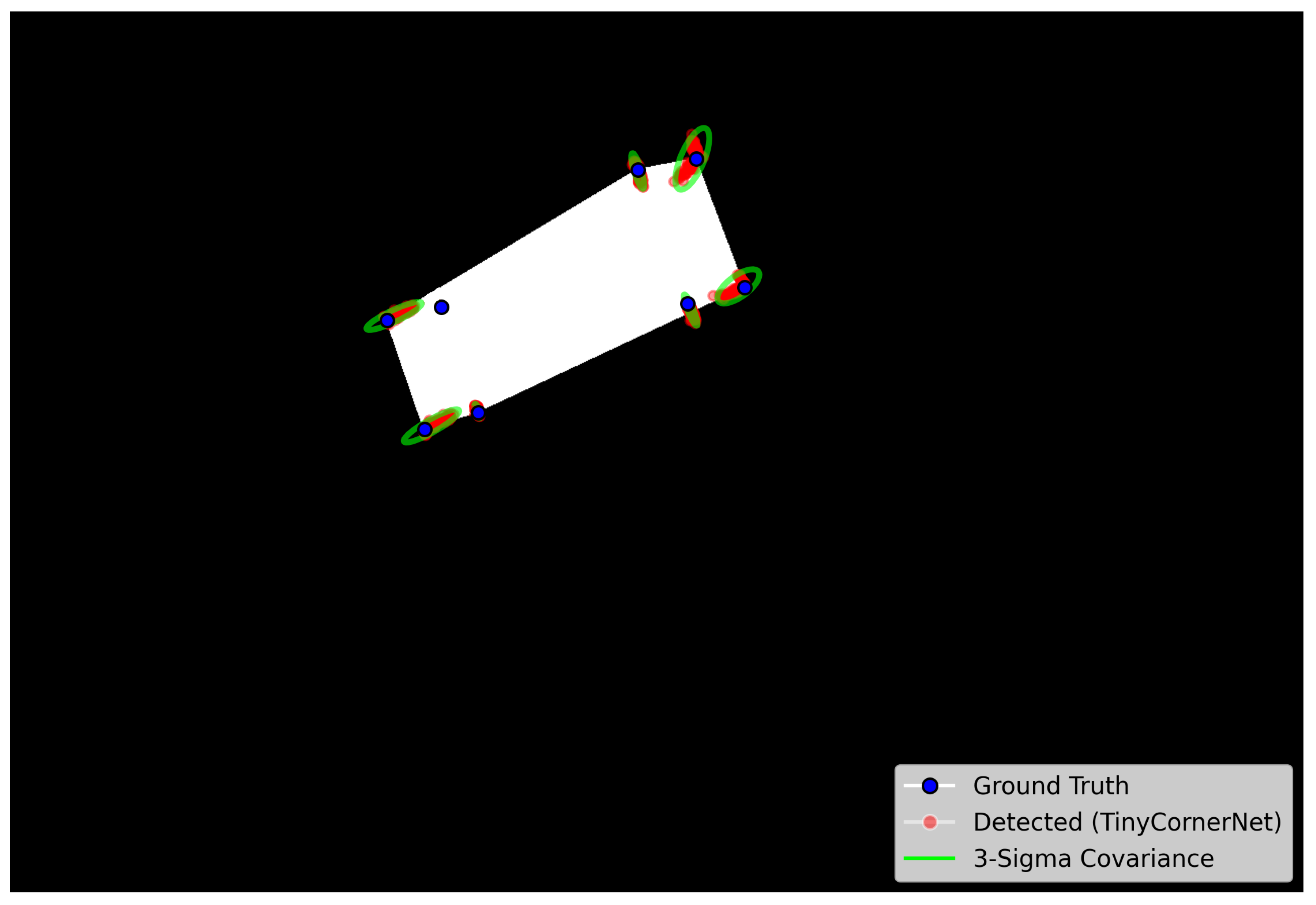
The resulting covariance matrix is integrated into the UKF initialization, ensuring the filter’s confidence in measurements. Figure 10 visualizes the CNN-detected marker spread around the ground truth for a sample image, where ellipses represent $3\sigma$ contours of the 2D covariance. Based on the TinyCornerNET detection statistics, the measurement noise covariance matrix for a single corner in 3D space was estimated through repeated randomized simulations. The resulting covariance captures the expected uncertainties, incorporating the effects of sensor noise, blur, and affine perturbations. The final estimated $\mathbf{R}$ matrix for a single corner is given as follows:

$${\mathbf{R}}_{SingleCorner}=\left[\begin{array}{ccc}4\times {10}^{-2}& 0& -2\times {10}^{-2}\\ 0& 1\times {10}^{-2}& 0\\ -2\times {10}^{-2}& 0& 4\times {10}^{-2}\end{array}\right]$$

(47)

As shown, the off-diagonal elements reveal a correlation between the x and z components, while the y-axis (depth) remains uncorrelated. This structure reflects the physical imaging characteristics where depth uncertainty arises independently from lateral uncertainties. Since each satellite corner marker is assumed to be independent, the full measurement noise matrix $\mathbf{R}$ for all markers is constructed by stacking the individual ${\mathbf{R}}_{\mathrm{Single}\mathrm{Corner}}$ blocks along the diagonal, forming a $21\times 21$ covariance matrix for the measurement vector when all visible markers are detected.

5.5. Markers Visibility

The presented measurement model relies on the positions of the eight corners of ENVISAT’s main body. However, the camera cannot capture all marker positions in a single frame because some markers are obscured by the ENVISAT’s structure itself. As a result, the filter cannot use the entire set of markers simultaneously; it has to adjust its measurements based on the visible markers. Consequently, the size of the measurement vector varies depending on the number of visible markers. Each marker provides three position measurements as an observation, so the measurement vector $\widehat{\mathbf{z}}$ will have $3·i$ components, where $i=0,\dots ,7$. The visible markers are located on the visible faces of the satellite, which are easier for the CNN to detect. Thus, the detection process focuses on identifying these visible faces for marker extraction. The requirement for face visibility is determined by the following equation:

$$\mathbf{u}·\mathbf{\Gamma }{\widehat{\mathbf{n}}}_i<0\mathrm{for}i={\psi }_1,\dots ,{\psi }_8$$

(48)

where ${\psi }_i$ defines the $i^{th}$ face of the main body. If the scalar product between the relative position vector of the chaser and the target $\mathbf{u}$ and the unit vector perpendicular to the face ${\widehat{\mathbf{n}}}_i$ is negative, it indicates that the face is oriented towards the camera, making the markers on that face visible. The filter uses the state information at the beginning of each observation to predict which markers will be visible in the next step, preparing to receive the correct number of measurements from the camera. The filter hardcodes the mapping between ENVISAT’s faces and the relative markers according to the vectors ${\widehat{\mathbf{n}}}_i$, thereby predicting marker visibility. The filter handles marker visibility in a binary manner, assigning a value of one if a marker is visible and zero if it is not, so that it can adapt the measurement dimensionality.

5.6. Marker Association

Once the CNN detects the potential marker positions, these measurements are compared to the predicted locations obtained busing Equation (44) for each marker through the filter’s estimated states. The association process is refined by minimizing the total distance between the predicted and measured positions. The total minimum distance is calculated using the Euclidean distance to ensure that the predicted marker locations are as close as possible to the measured ones. Mathematically, this operation can be shown by constructing a cost function, J, that minimizes the squared distance between the predicted marker locations, ${\mathsf{ø}}_j$, and the measured marker locations, ${\mathbf{\Xi }}_i$. The cost function J selects the pairings $(i,j)$ that minimize the total squared distance, effectively associating each predicted marker to the closest measured marker. This can be formulated as follows:

$$J=arg\underset{i,j}{min}\sum _{i,j}{({\mathbf{\Xi }}_i-{\mathsf{ø}}_j)}^2$$

(49)

Figure 11 visually demonstrates the marker association process that uses the previous equation to match the specific markers with the corners.

Dashed yellow lines represent the distance to the second-closest corner, while the orange solid line shows the shortest path to a specific corner. The marker association optimization ensures that the markers identified by the CNN are associated with the correct position vector ${\mathbf{v}}_i$.

6. Numerical Results

Before discussing the results of this work, it would be appropriate to give an end-to-end pipeline for summarizing all components until this point. Therefore, Figure 12 provides a pipeline diagram of the method discussed in this work. Moreover, as shown in Figure 9, ENVISAT’s center of mass is separated from the geometric center, located closer to one of the solar panel sides. This asymmetry in the density creates robustness in the marker association for the initial and transient parts of the filtering simulation.

Note that in the estimation framework, initial uncertainties are accounted for by introducing random noise into all states. Specifically, a standard normal distribution is applied to these states, with varying levels of uncertainty to reflect their initial conditions, which are given in

Table 2. Initial conditions.

Translational Dynamics		Rotational Dynamics
x (m)	−0.002	$\varphi$ (roll,rad)	1.66
y (m)	−31.17	$\theta$ (pitch,rad)	2.27
z (m)	0	$\psi$ (yaw,rad)	−0.38
$\dot{x}$ (m/s)	−3.5 × 10−6	${\omega }_x$ (rad/s)	0.02
$\dot{y}$ (m/s)	−2.0 × 10−6	${\omega }_y$ (rad/s)	0.02
$\dot{z}$ (m/s)	0	${\omega }_z$ (rad/s)	0.04

. For the position state, a normal distribution with a standard deviation of 1.0 is used, indicating relatively high uncertainty in the initial position estimation. The velocity state is subjected to a tighter distribution with a standard deviation of $1.0\times {10}^{-1}$. Similarly, the MRPs, representing the satellite’s attitude, are modeled with a normal distribution with a standard deviation of $1.0\times {10}^{-2}$, indicating moderately high uncertainty in the initial orientation. Lastly, the angular velocity state is assigned a standard deviation of $1.0\times {10}^{-3}$. The parameters for the UKF are selected as follows: $\alpha =0.25$, $\beta =2.0$, and $\kappa =3.0$. These values are chosen based on standard guidelines for UKF performance and system dynamics. All other simulation-related parameters, such as the inertia tensor and mass of ENVISAT, are taken from the literature [50].

Our initial findings demonstrate promising outcomes in the detection and analysis of structural markers on the ENVISAT satellite through processed imagery. This approach not only enhances the robustness of our detection algorithms under varied operational scenarios but also aligns with the typical image quality captured by space-borne sensors. Each simulated image undergoes a preprocessing phase where Gaussian noise and blur are applied to prove the robustness and performance of the software. The addition of Gaussian noise is intended to mimic the electronic noise and sensor imperfections typically found in spacecraft imaging systems. This noise simulates the random variations in pixel intensity that occur due to various factors. Simultaneously, a Gaussian blur was applied to replicate the blurring effect caused by minute focusing discrepancies or motion effects that can occur in a spacecraft’s optical system [12].

Table 3. Camera intrinsic properties and simulation parameters.

Parameter	Value
$FoV$ (Field of view)	45 (degree)
$f_x$ (Focal length in x-direction)	1280 (pxs)
$f_y$ (Focal length in y-direction)	1280 (pxs)
$c_x$ (Principal point x-coordinate)	640 (pxs)
$c_y$ (Principal point y-coordinate)	640 (pxs)
Affine translation (std. dev.)	3 pixels (in both x and y)
Affine rotation (std. dev.)	1 (degree)

shows the camera and simulation parameters selected within this study.

Figure 13 demonstrates the preliminary results of a CNN algorithm. After marker identification, the measurements coming from the CNN algorithm are fed into the UKF framework as the measurements of the filter for the relative pose estimation. As a reminder, it is assumed that a priori knowledge of the geometrical and physical characteristics of both chaser and target is available, with rigid body dynamics, and that the chaser motion is deterministic and without external disturbances or control actions. The camera cannot detect all marker positions in a single frame because parts of ENVISAT’s structure obscure some markers. Consequently, the filter does not operate with the entire set of markers but adjusts its measurements frame-by-frame based on which markers are visible. The visibility and correct association of a corner to its corresponding marker are crucial, as locating more markers tends to enhance the estimation accuracy since it increases the observability of the system. Moreover, the presence of Gaussian noise and blur in the measurements further exacerbates the degradation in estimation quality. These factors introduce additional variability and error into the measurements, which in turn affect the overall accuracy of the position and orientation estimates.

In order to understand the effects of measurement noise and the number of visible markers, Monte Carlo runs were executed within the UKF framework. Note that in all Figure 14, Figure 15 and Figure 16, the red dashed lines represent the three sigma values from the updated error covariance matrix of the filter, the solid blue lines are the three sigma values obtained from the sampled errors of the Monte Carlo, and the gray lines are single Monte Carlo runs of the simulation. The effective (sampled) errors are computed as the root-sum-square (RSS) differences between the true states and the estimated mean states. Note that the effective error of the Monte Carlo simulation represents the actual error spread of the filter, calculated by running multiple simulations with different initial conditions. The estimated errors, derived from the covariance matrix, are computed as the square root of the sum of the diagonal elements corresponding to the filter states. The difference can be obviously seen in Figure 14 and Figure 15, where the standard deviation of the measurement noise (zero-mean Gaussian) for the sensors is increased from $0.02$ to $0.2$. These values are selected to simulate mild to moderate noise on digital, simulated images. This dual impact of fewer markers and increased noise highlights the challenges in accurately determining the satellite’s state under suboptimal conditions. These results underscore the importance of maximizing the number of observed markers and minimizing noise to achieve high-quality estimation of the satellite’s relative position and orientation. Finally, in Figure 16, it is evident that with fewer markers observed throughout the time period, the estimation accuracy is also decreased.

Again, in Figure 14, Figure 15 and Figure 16, the red dashed lines represent the three-sigma values derived from the estimated error covariance matrix, and the blue lines show that the effective three-sigma values obtained from the sampled errors are close to each other and encapsulating the Monte Carlo errors. Consequently, the UKF has performed well, maintaining estimation accuracy despite the challenges posed by reduced marker observations and other uncertainties in the simulation, such as the measurement noise on the sensors. The filter is able to predict its own uncertainties, and the initial large error covariance is reduced rapidly to steady-state values. Indeed, to show convergence, the figures are zoomed around the steady state, while the initial large uncertainties are out of the graph (for visualization purposes). The error spikes are visible around some points, especially for the rotational position and velocity errors. The fundamental reason behind this phenomenon is the positioning of ENVISAT in the camera frame and its orientation, which reduces observability. It is important to state that the filter robustness and accuracy are sensitive to the filter frequency, which is set at 1 Hz for this study. The filter tends to perform less accurately below this frequency threshold, while it stays convergent above this frequency due to the sampling rate and discretization errors.

Robustness to Missing Observations: The Eclipse

For the ENVISAT satellite, the eclipse duration was calculated to be 35.57 min. This eclipse occurs when the satellite passes into the Earth’s shadow, during which the Sun’s light is blocked, and no direct sunlight reaches the satellite. Regardless of possible detection due to other light sources, it has been assumed to be a worst-case scenario where, during this eclipse period, the corners and markers of the satellite will never be visible to the cameras used for measurement. As a result, there will be no measurement updates in the UKF during this time. The UKF relies on visual tracking to update the satellite’s state estimates, and without sufficient visibility, the necessary data for these updates will be unavailable. Therefore, during the eclipse period, the estimation process will continue without measurement updates, relying solely on the prediction step to propagate the relative pose uncertainties. Figure 17 visualizes the eclipse phase where the Sun is inserted far away in the $-X$ axis.

In order to mitigate the impact of missing measurements and maintain estimation quality, we introduce and adjust the process noise covariance matrix $\mathbf{Q}$ during the eclipse, which starts around the 2000th s of the simulation and continues for approximately 35.57 min. While measurements are unavailable, the fidelity of the uncertainty estimate is merely based on the propagation step. In an ideal scenario, the predicted PDF, approximated as Gaussian by the UKF, perfectly describes the true non-Gaussian PDF, whose shape is unknown. In order to not lose custody of the target with an extreme confident success rate, the UKF predicted covariance needs to guarantee that the full uncertainties of the true PDF are enclosed in its prediction. This aspect is achieved through covariance inflation to ensure that the algorithm counteracts distributions with long tails and many outliers, which usually results from highly nonlinear dynamics (such as ENVISAT’s). The matrix $\mathbf{Q}$ reflects uncertainties in the system dynamics, and increasing its values during the eclipse according to the covariance-inflating methodology helps to ensure that the predicted uncertainty adequately encompasses the potential spread of the state. This inflation prevents the filter from becoming overconfident in its predictions and helps retain robustness under high nonlinearity and absent measurements. As the system is highly nonlinear, and the distribution becomes non-Gaussian, the noise inflation prevents degeneracy from outlier observations or states, providing robustness from every possible revelation. As shown in the results, the covariance inflation guarantees that every possible Monte Carlo simulation, not just in a $3\sigma$ boundary sense, is enclosed in the uncertainty to guarantee that the UKF does not lose fidelity and custody of the target. Once the satellite exits the Earth’s shadow and the eclipse ends, measurement updates resume, and the UKF rapidly reduces accumulated prediction error by incorporating sensor data. To assess the filter’s consistency under these conditions, Monte Carlo simulations were conducted. Figure 18 compares estimated covariances for eclipse and no-eclipse cases, where solid blue lines denote three-sigma bounds from the estimated covariance under eclipse, red dashed lines represent the no-eclipse case, and gray lines show the Monte Carlo errors. In Figure 19, Figure 20, Figure 21 and Figure 22, red dashed lines show three-sigma values from the sampled errors, solid blue lines represent the three-sigma values from the estimated covariance, black lines show the mean error, and gray lines denote the Monte Carlo realizations.

The results demonstrate that the filter remains consistent and accurate in tracking the satellite’s state under nominal conditions. Notably, during the eclipse period, when no measurements are available because of the occlusion of satellite markers, an adjustment of the process noise covariance matrix is implemented. Despite the lack of direct measurement updates during the eclipse, the Monte Carlo errors remain within the expected bounds, indicating that the $\mathbf{Q}$ adaptation preserves the filter’s accuracy and robustness throughout the eclipse period. The matrix $\mathbf{Q}$ is a diagonal matrix in which each diagonal element represents the process noise for a specific state of the system. The first three values $(0,0,0)$ correspond to position states and have negligible process noise. The next three values $(2\times {10}^{-14})$ are for the translational velocity states, reflecting low uncertainty. The following three values $(8\times {10}^{-14})$ are for the rotational states, represented by the MRPs, indicating higher uncertainty. The last three values $(5\times {10}^{-14})$ correspond to the rotational velocity states, with moderate uncertainty. This diagonal structure allows for independent control of the noise levels for each state.

Table 4. Diagonal values of the $\mathbf{Q}$ matrix, categorized by position, velocity, angular position, and angular velocity blue used during the eclipse.

State	Standard Deviation
Position (x, y, z)	0, 0, 0 (m)
Velocity (${\mathbf{v}}_{\mathit{x}}$, ${\mathbf{v}}_{\mathit{y}}$, ${\mathbf{v}}_{\mathit{z}}$)	$2\times {10}^{-14}$, $2\times {10}^{-14}$, $2\times {10}^{-14}$ (m/s)
Angular Position (${\mathbf{r}}_{\mathit{x}}$, ${\mathbf{r}}_{\mathit{y}}$, ${\mathbf{r}}_{\mathit{z}}$)	$8\times {10}^{-14}$, $8\times {10}^{-14}$, $8\times {10}^{-14}$ (rad)
Angular Velocity (${\mathit{\omega }}_{\mathit{x}}$, ${\mathit{\omega }}_{\mathit{y}}$, ${\mathit{\omega }}_{\mathit{z}}$)	$5\times {10}^{-14}$, $5\times {10}^{-14}$, $5\times {10}^{-14}$ (rad/s)

shows the diagonal values of $\mathbf{Q}$.

Beyond the eclipse situation, we also ran a Monte Carlo analysis for a case without any eclipse. This helped us establish a consistent point of comparison. It is available on Appendix A section of this study.

7. Discussion

This paper presents a robust approach to relative pose navigation for the tumbling ENVISAT spacecraft, emphasizing the online collaboration between a filter and a CNN-based image processing camera. As part of this study, we introduce TinyCornerNet, a lightweight CNN specifically designed for robust corner detection in spaceborne imagery. Unlike large-scale models, TinyCornerNet achieves high accuracy while maintaining computational efficiency, making it well-suited for onboard or real-time processing. Its architecture was optimized to reliably detect structural markers on satellite targets under various noise and distortion conditions. The results demonstrated that TinyCornerNet outperforms traditional corner detectors in both accuracy and robustness. In each cycle, the CNN processes the incoming images to extract corner measurements, which the filter then uses to predict and update the uncertainty of the system. Overall, the proposed pipeline not only addresses the complexity of autonomous rendezvous with a non-cooperative target but also lays a foundation for future advancements in space debris monitoring and active removal. Additionally, a key contribution of this work is the adjustment of the process noise covariance matrix via covariance inflation during eclipse periods. This adaptation ensures the continued accuracy of the UKF, allowing it to maintain state estimation despite the absence of direct sensor updates. Monte Carlo simulations, with and without eclipse scenarios, demonstrate the robustness and consistency of the proposed method. In eclipse conditions, the $\mathbf{Q}$ adjustment effectively compensates for the uncertainty introduced by the lack of measurements, keeping estimation errors within expected bounds. The reason is that $\mathbf{Q}$ represents the uncertainty in the system’s dynamics, specifically the degree to which the model’s predictions may diverge from the true state due to unmodeled/unknown or highly nonlinear dynamics, disturbances, or inaccuracies in the dynamic model. By increasing the values in $\mathbf{Q}$ during the eclipse, the filter acknowledges the higher spread of uncertainty and adjusts its predictions accordingly. A higher $\mathbf{Q}$ value increases the predicted state covariance, allowing the filter to reflect the potential range of error in its predictions more accurately. This prevents the filter from becoming overly confident in its predictions, thus mitigating the risk of large deviations between the predicted and true states. Once measurements are available again, the filter can quickly recover, reducing the accumulated uncertainty and maintaining overall consistency. The scenario without an eclipse confirms the filter’s nominal performance with continuous measurements. These findings suggest that the proposed approach offers a scalable, reliable solution for space debris management and contributes significantly to the advancement of autonomous de-orbiting systems.

In future work, we plan to integrate the CNN module directly within the UKF framework to further refine the pose estimation and tracking of space objects. This integration aims to overcome the limitations of current tracking systems by providing more accurate, rapid, and reliable state estimation under the complex and dynamic conditions of space environments. Moreover, the UKF will be improved by trying to implement an online adaptation of the measurement noise matrix rather than putting it into a constant matrix, which is reported to improve the quality of the estimation in different studies [51,52,53]. Future work should also focus on incorporating stochastic absolute values into the estimation process and enhancing the interaction between the camera system and the filter. Introducing stochastic elements can account for uncertainties and variabilities in absolute measurements, thus improving the robustness and accuracy of state estimation. Future work will involve using the full ENVISAT model with all its detailed features (solar panels, body panels, etc.). We will test the corner detection performance under these more realistic conditions to better evaluate the robustness of our method. Additionally, optimizing the interaction between the camera system and the filter can lead to more efficient processing, allowing the filter to guide the camera in focusing on specific regions of interest, thus reducing computational load and improving real-time performance.