Article

Wide-Range Variable Cycle Engine Control Based on Deep Reinforcement Learning

1
School of Aerospace Engineering, Xiamen University, Xiamen 361102, China
2
Aero Engine Academy of China, Beijing 101304, China
*
Author to whom correspondence should be addressed.
Aerospace 2025, 12(5), 424; https://doi.org/10.3390/aerospace12050424
Submission received: 23 March 2025 / Revised: 6 May 2025 / Accepted: 7 May 2025 / Published: 10 May 2025

Abstract

:
In this paper, a controller design method based on deep reinforcement learning is proposed for a wide-range variable cycle engine with a turbine interstage mixed architecture. The PID controller is subject to limitations, including single-input single-output limitations, low regulation efficiency, and poor adaptability when confronted with contemporary variable cycle engines that exhibit complex and multi-variable operating conditions. To solve this problem, this paper adopts a deep reinforcement learning method based on a deep deterministic policy gradient algorithm, and it applies an action space pruning technique to optimize the controller, which significantly improves the convergence speed of network training. In order to verify the control performance, two typical flight conditions are selected for simulation experiments as follows: in the first scenario, H = 0 km and Ma = 0, while in the second scenario, H = 10 km and Ma = 0.9. A comparison of the simulation results shows that the proposed deep reinforcement learning controller effectively addresses the engine’s multi-variable coupling control problem. In addition, it reduces response time by an average of 44.5%, while maintaining a similar overshoot level to that of the PID controller.

1. Introduction

The Variable Cycle Engine (VCE) is a revolutionary aircraft engine that utilizes a sophisticated system to regulate its thermodynamic parameters. This system involves the manipulation of the engine’s variable geometry components, altering their shape, size, and position. The primary objective of this innovation is to expand the engine’s operational speed range, ensuring optimal performance across a wide spectrum of flight regimes, including subsonic, transonic, supersonic, and even hypersonic speeds. In comparison to conventional engines, variable cycle engines are characterized by higher specific thrust, greater circulation capacity, and a broader operational speed range. For this reason, they are a primary focus of aerospace engineering research [1,2].
Since the introduction of the VCE concept by General Electric in the 1960s, significant advancements have been made in the field of variable cycle engines [3]. Typical VCE configurations include the single-externality VCE [4], the double-externality VCE with a core-driven fan stage [5,6], and the triple-externality VCE [7,8]. Compared to the multi-external VCE, the single-externality VCE has relatively fewer variable geometry components. Among them, the Interstage turbine mixed architecture (ITMA) of the single-externality variable cycle engine has received special attention due to its unique advantages. A comparative study in the literature [9] shows that this configuration exhibits a 12.75% reduction in fuel consumption at subsonic cruising speeds, accompanied by exceptional propulsive efficiency. Consequently, it is anticipated that this configuration will serve as the primary architectural framework for the subsequent generation of fighter variable cycle engines. This makes it one of the main architectures for the next generation of variable cycle engines for fighter aircraft.
The integration of variable geometry components within the ITMA architecture has been demonstrated to enhance performance, yet it concomitantly introduces challenges related to control. A systematic study in the literature [10] points out that there are strong nonlinear dynamic characteristics and strong coupling effects when the engine operating conditions change. These phenomena result in the performance limitations of traditional control methods, such as PID control. To address this challenge, artificial intelligence has been shown to have unique advantages. The successful application of neural networks in robot control has been documented in the literature [11,12]. The breakthrough of AI technology in UAV anti-jamming has been demonstrated in the literature [13,14]. The innovative practice of deep reinforcement learning in multi-objective optimization for autonomous driving has been described in the literature [15,16]. In particular, the efficacy of reinforcement learning technology, a field of artificial intelligence that is currently experiencing significant research activity, in addressing multi-constraint problems of nonlinear systems has been substantiated through theoretical analyses documented in the extant literature [17]. The deep reinforcement learning (DRL) framework proposed in the literature provides a novel paradigm for complex control systems [18,19].
As demonstrated in the extant literature, the DRL method has been shown to be a highly adaptable intelligent control method. It has been determined to be particularly suitable for aero-engine systems that exhibit strong nonlinearity, multi-variate coupling, and high-dimensional dynamic characteristics [20]. Consequently, numerous scholars have employed this methodology in the domain of aero-engine control, attaining noteworthy outcomes. For example, Zheng et al. [21] proposed a control system for a conventional turbofan engine that was designed using an online Q-learning algorithm, with an online sliding window deep neural network used to estimate the action value function. Liu et al. [22] have investigated the reinforcement learning control of a variable geometry inlet aspirated hypersonic vehicle based on the Lyapunov function. The transition process control of turbofan engines was addressed by Fang et al. [23], who applied deep reinforcement learning across the entire flight envelope through similarity transformation methods. Tao et al. [24] designed a multi-variable control law for a variable cycle engine and employed deep reinforcement learning algorithms to online optimize the control law, resulting in a fuel consumption rate lower than that achieved by traditional optimization algorithms. Gao et al. [25] employed the Deep Deterministic Policy Gradient (DDPG) algorithm to construct a controller for the transition process of a typical turbofan engine. Additionally, a complementary integrator was introduced to mitigate the steady-state error caused by the approximation error of the deep neural network. However, the majority of the aforementioned DRL research is grounded in the domain of ordinary turbofan turbojet engines. Consequently, there is fewer research focusing on the implementation of DRL in complex control systems for wide-area variable-cycle engines.
In summary, DRL has become an important research direction in the field of aero-engine control, owing to its ability to address complex nonlinearities, multi-variate coupling, and high-dimensional dynamic characteristics. Specifically, the ITMA engine architecture demonstrates considerable promise for advancement; however, the implementation of DRL control methodologies in complex, variable-cycle engine control systems remains under-explored. In this paper, a DRL controller is developed for the ITMA engine control problem. This controller is based on the deep deterministic policy gradient algorithm and action space pruning method. These techniques solve the single-input single-output limitation of the PID controller as well as the coupling between control quantities. At the same time, this controller improves the response speed of the engine during acceleration and deceleration.
The primary contributions of this paper are as follows:
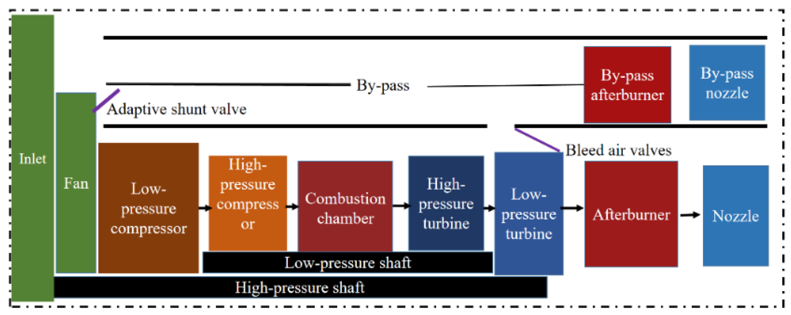
  • A methodology for the design of controllers is proposed. This methodology is based on deep reinforcement learning. The objective of this methodology is to address the complex control problem associated with a wide-area variable-cycle engine that features an interstage turbine mixed architecture.
  • The Deep Deterministic Policy Gradient (DDPG) algorithm is employed to effectively address the nonlinearity, multi-variable coupling, and high-dimensional dynamic characteristics of variable cycle engines.
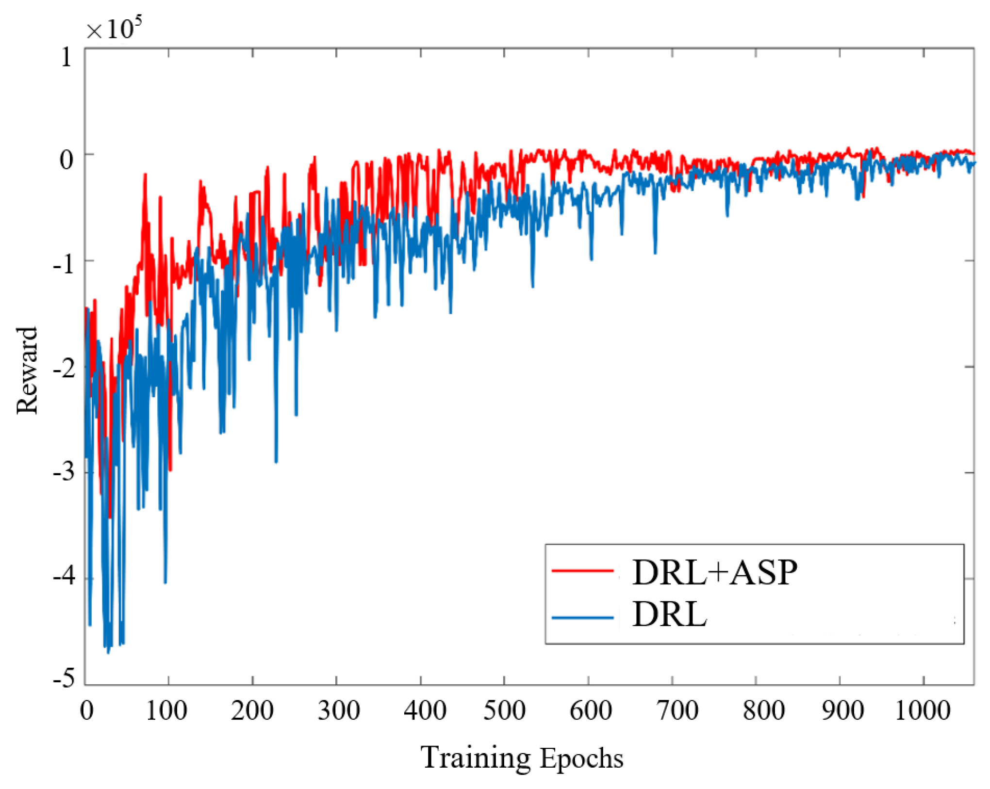
  • Combined with the action space pruning technique, the performance of the controller is optimized and the convergence speed of training is improved. The efficacy of the method in addressing multi-variate coupling problems is substantiated by simulation verification.
The rest of the paper is organized as follows: Section 2 introduces the preliminary knowledge and the mathematical description of the problem in this paper; Section 3 combines the methods of deep reinforcement learning and action space pruning to design the DRL controllers; Section 4 gives the corresponding simulation results and their analysis; and Section 5 concludes the paper.

2. Preliminary Knowledge and Problem Description
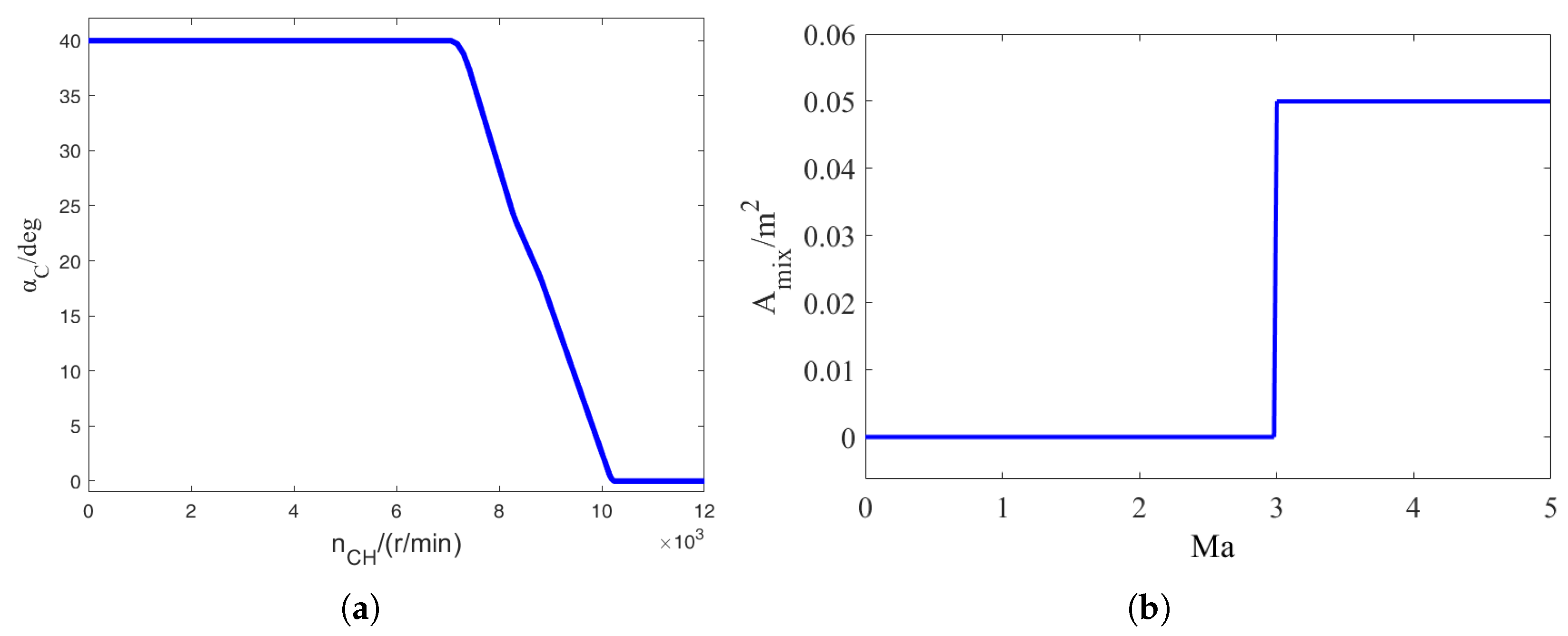
2.1. Study Objects

Figure 1 shows a wide-range variable-cycle engine architecture of the Interstage Turbine Mixed Architecture (ITMA), consisting of an inlet duct, fan, compressor, turbine, combustion chamber, and tailpipe. The architecture employs a multi-stage low-pressure turbine configuration to achieve a higher low-pressure turbine expansion ratio, thereby improving engine airflow and reducing fuel consumption. Furthermore, the single-container configuration of the ramjet stage, in conjunction with the distinct exhaust architecture of the inner and outer containers, effectively decouples the fan from the nozzle. Increasing the fan speed at high Mach numbers enables the fan to operate at a more optimal operating point. Finally, the internal and external bleed air intake area is employed for the interstage turbine mixed architecture. This process serves to mitigate mixing losses and regulate the low-pressure turbine airflow to enhance its efficiency. This architecture has been shown to enhance propulsive efficiency during subsonic flight, and it demonstrates excellent performance during supersonic cruise [9]. A description of the symbols used in this paper for ITMA engines is given in Table A1.
Engine control is achieved by adjusting several adjustable variables during the operation of the ITMA wide-range variable cycle engine. The aforementioned variables encompass the following: the main combustion chamber fuel flow rate denoted by w f , the fuel flow rate of the afterburning chamber denoted by w f , a f t e r , the guide vane angle of the high-pressure compressor denoted by α C , the nozzle throat area denoted by A 8 , the bypass nozzle throat area denoted by A 8 , o u t e r , and the internal and external bleed air intake area denoted by A m i x . The range of parameter variation for these variables is demonstrated in Table 1.
The ITMA engine control system is designed to ensure that the pilot is able to move the throttle stick unrestrictedly over the entire engine operating envelope without causing surge, over-temperature, over-rotation, or exceeding of the operating limits. In order to accomplish this, the reference command values corresponding to each throttle stick position must be calculated. The engine operates in the full speed domain and the culvert ratio is approximately 0.6 under most working conditions. As a result, the low-pressure relative speed, denoted by n R L , is designated as one of the controlled quantities. Secondly, the nozzle throat area, designated as A 8 , exerts a direct influence on the flow rate, thrust output, and efficiency of the core engine. Consequently, the connotation drop ratio, denoted by π , is selected as the second controlled quantity. The regulation of the bypass nozzle of the ITMA engine is also crucial. This regulation plays a dual role as follows: it prevents the occurrence of the surge phenomenon and directly affects the engine’s thrust and the fuel consumption rate, so the outer culvert boost ratio, denoted by π B , is the third controlled quantity. Therefore, the indirect control of the thrust is realized by controlling n R L , π , and π B . The above variables are represented as follows:
n R L = n L / 288.15 / T t 2 ( n L / 288.15 / T t 2 ) d
π = P t 6 P s 31
π B = P t 16 P t 0
where n L is the fan speed, T t 2 is the engine intake temperature, P t 6 is the post-turbine pressure, P t 16 is the pre-afterburner chamber pressure, P s 31 is the high-pressure post-compressor pressure, and P t 0 is the atmospheric static pressure. The subscript d denotes the operating point on the compressor characteristic curve.

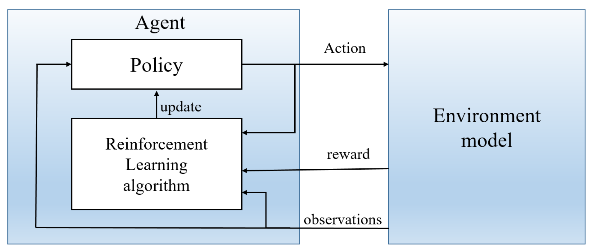
2.2. Overview of Deep Reinforcement Learning

Reinforcement learning aims to learn the optimal policy during the continuous interaction between the agent and the environment so as to generate the best sequence of actions for obtaining the maximum reward. In this process, the main components are the agent and the environment model. In the framework shown in Figure 2, the environment is a place where the agent’s actions take effect and generate rewards and observations. The agent consists of a policy and a learning algorithm. The policy is a function that maps observations to actions, and the learning algorithm is an optimization method used to find the policy.
THe Markov Decision Process (MDP) is a theoretical framework for reinforcement learning. The agent selects the corresponding action a t A ( s ) , and S and A ( s ) are the set of states and the set of actions, respectively, based on the observed state of the environment s t S at a discrete time t. After executing the action, the agent will observe the new state s t + 1 and reward r t R at the next moment. Based on the above information, a history trajectory h t = [ s 0 , a 0 , r 1 , s 1 , a 1 r t , s t ] T can be obtained and the state transfer probability at moment t + 1 is calculated P ( s | s , a ) .
P ( s | s , a ) = P r ( s t + 1 = s , a t = a | s t = s , a t = a )
The rewards are defined as
G t = t = 0 γ t r t + 1
where γ [ 0 , 1 ] is the discount factor, which indicates how much future rewards are discounted from current rewards. Higher discounts indicate a greater emphasis on future rewards.
Policy π ( a | s ) determines the selection probability of the next action based on the current state s t = s . Its computation is based on the state value function V π ( s ) and the action value function Q π ( s , a ) . The state value function V π ( s ) is defined as the expected cumulative reward when starting from state s and following policy π .
V π ( s ) = E a π ( · | s ) R ( s , a ) + γ s P ( s | s , a ) V π ( s )
The expected reward when taking action a in state s and then acting according to policy π is the action value function Q π ( s , a ) as follows:
Q π ( s , a ) = E s P ( · | s , a ) R ( s , a , s ) + γ a π ( a | s ) Q π ( s , a )
The ultimate goal of reinforcement learning is to find an optimal policy π * that maximizes the cumulative reward of taking that policy in any state. The optimal policy satisfies the following:
π * ( s ) = arg max a Q * ( s , a )
The optimal equation under the optimal policy can be expressed as follows:
V * ( s ) = max π V π ( s )
Q * ( s , a ) = max π Q π ( s , a )
DRL combines Deep Learning and Reinforcement Learning by approximating the value functions, policy functions, etc. in Reinforcement Learning through deep neural networks to cope with more complex environments and tasks. The difference between DRL and Reinforcement Learning is that the value functions or policy functions in Reinforcement Learning are represented through tabular methods or linear models, and DRL approximates these functions through deep neural networks.

2.3. Description of the Problem

The engine thrust demand is the reference command for the main control loop, which is obtained by calculating the throttle stick position set by the pilot. Considering the reason that the engine thrust is not measurable in practical applications, the indirect control of thrust is realized by controlling n R L , π , and π B in conjunction with the performance requirements of the engine operation.
In addition, modern aero-engines require the control system to ensure the stability and optimal solution of the engine working state. This system is also responsible for adhering to the safety constraints of the aerodynamic stability and strength. These constraints specifically encompass the following: the relative rotational speeds of high and low pressure must be maintained at a maximum of 105%, and the pre-turbine temperature must be maintained at a maximum of 1750 K. It is imperative that the high-pressure pressurized gas turbine surge margins, denoted by S M C , and the fan surge margins, denoted by S M F , are maintained at a minimum of 5%. Consequently, the objective of this study is to design a controller that will address the following problems:
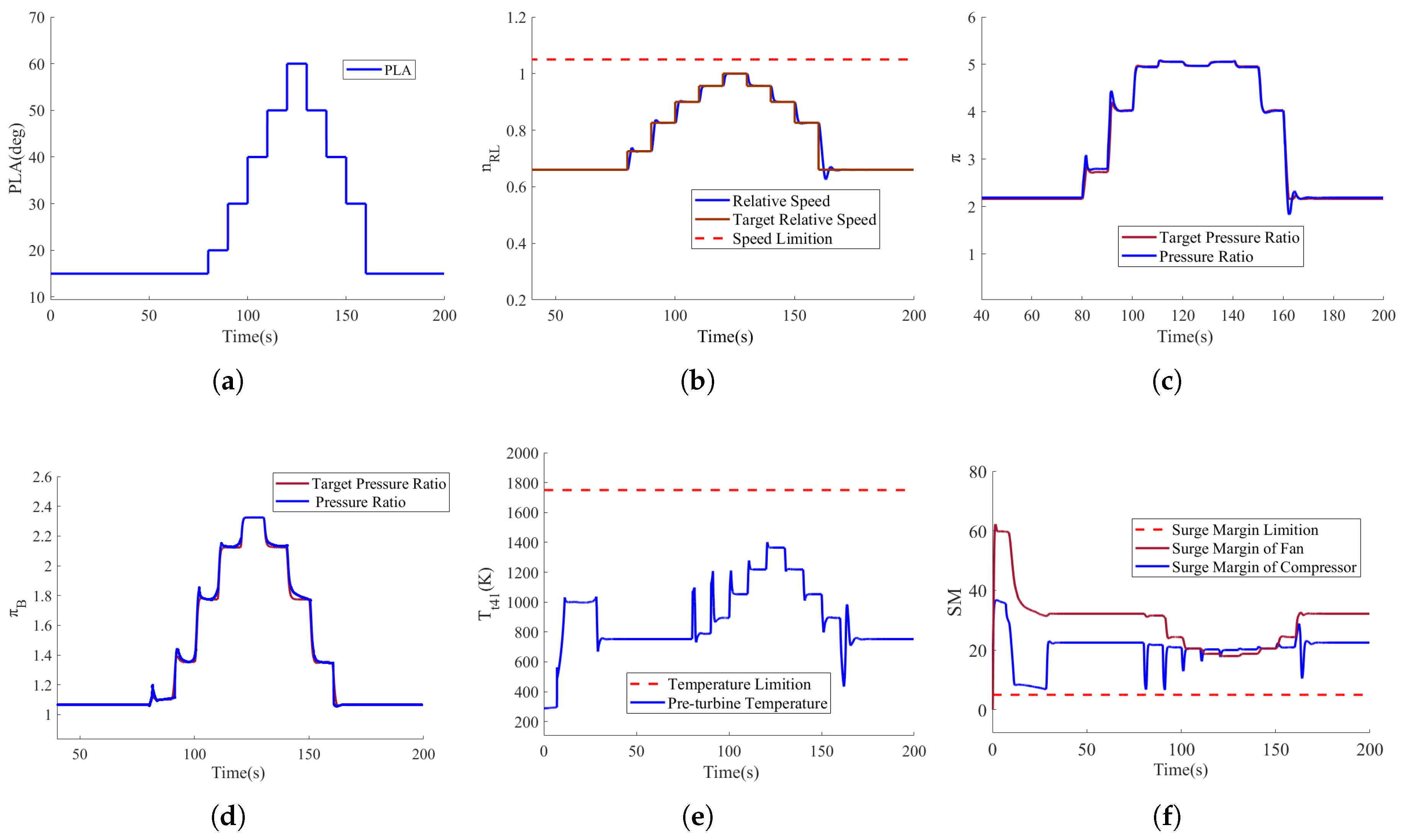
  • (2.3a) Speed tracking control: Ensure that the tracking error of the the low-pressure relative speed eventually converges to zero.
  • (2.3b) Connotation drop ratio tracking control: Ensure that the tracking error of the connotation drop ratio eventually converges to zero.
  • (2.3c) Outer culvert boost ratio tracking control: Ensure that the tracking error of the outer culvert boost ratio eventually converges to zero.
  • (2.3d) Limiting protection control: No over-temperature, over-rotation, or surge occur under any flight condition.
We define the tracking error of the engine as follows:
δ n R L =   | n R L , cmd n R L | δ π =   | π cmd π | δ π B =   | π B , cmd π B |
where δ n R L , δ π , and δ π B denote the deviation between n R L , π , and π B and their respective target instructions.
The mathematical description of the specific problem is as follows. We design feasible control laws that allow the engine to be operated in different flight environments by adjusting μ t = [ W f , A 8 , A 8 , o u t e r , w f , a f t e r , α C , A m i x ] , so that the following holds:
lim t δ n R L = 0 lim t δ π = 0 lim t δ π B = 0 ,
and,
S M C 5 % S M F 5 % T t 41 1750 K n R H 1.05 n R L 1.05 .
The thrust tracking control problem of the ITMA engine is transformed into the multi-variate tracking control problem with the aforementioned constraints. In order to solve this problem, this paper adopts a DRL approach to solve the multi-variate tracking control problem by utilizing its idea of learning optimal strategies.

3. Design of the Deep Reinforcement Learning Controller

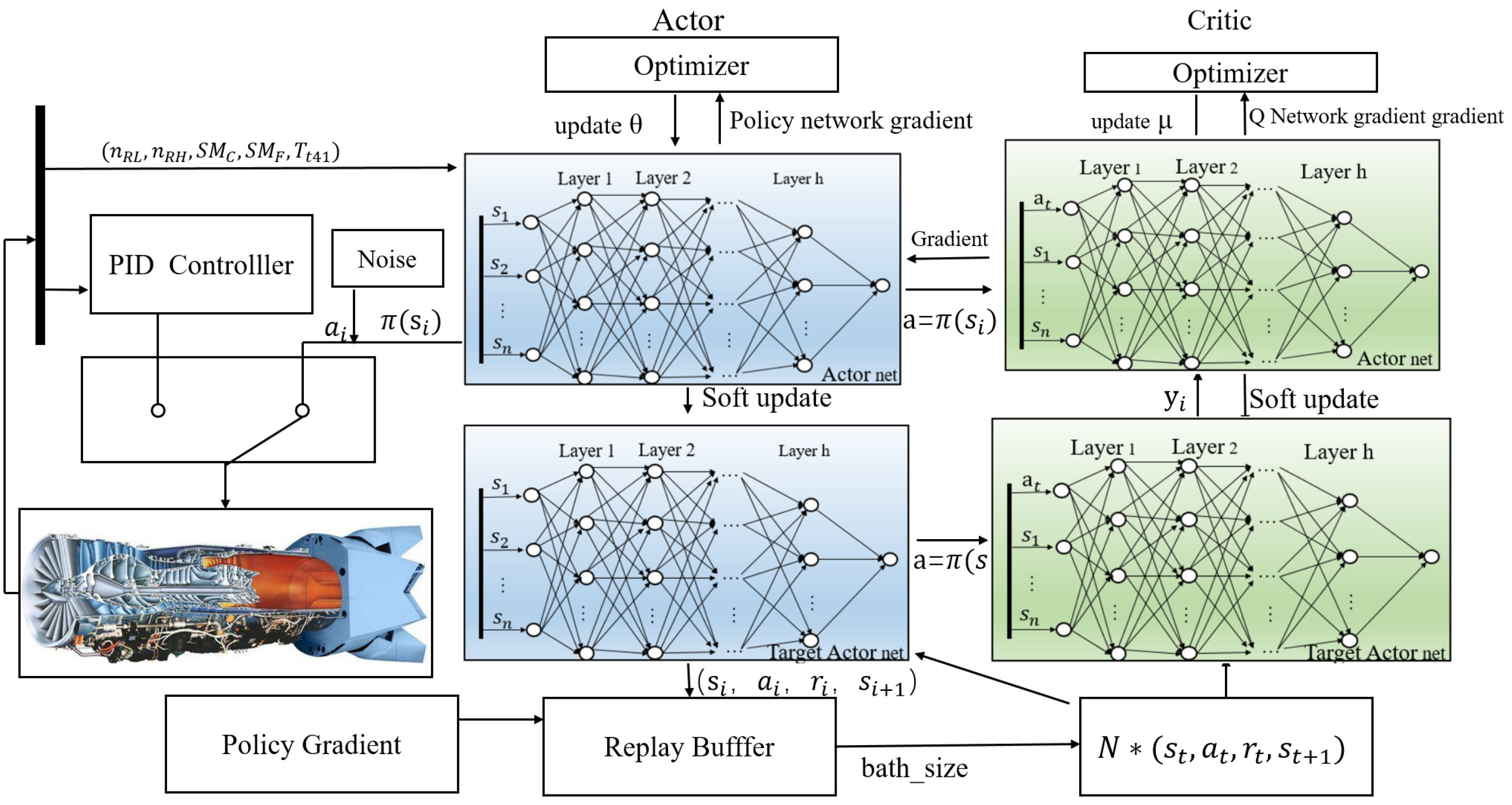
3.1. Control System Structure

The controller outputs of the ITMA engine are six variables, namely, the main combustion chamber fuel flow w f , fuel flow of the afterburner w f , a f t e r , guide vane angle of the high-pressure compressor α C , nozzle throat area A 8 , bypass nozzle throat area A 8 , o u t e r , and internal and external bleed air intake area A m i x .
In the engine control process, we employ a hierarchical control architecture to precisely regulate the key parameters. The core control loop achieves the tracking control of the low-pressure relative rotational speed n R L , connotation drop ratio π , and outer culvert boost ratio π B by adjusting w f , A 8 , and A 8 , o u t e r . Simultaneously, α C , w f , a f t e r , and A m i x are regulated to ensure the engine operates within safe operating limits. Therefore, w f , A 8 , and A 8 , o u t e r are controlled in a closed-loop manner, with the DRL control strategy primarily focuses on learning and optimizing w f , A 8 , and A 8 , o u t e r . The overall control block diagram is shown in Figure 3.
The afterburner has specific operating conditions, outlined as follows: it only activates when the ambient pressure reaches a preset threshold and the throttle angle P L A exceeds 75 deg. w f , a f t e r is obtained by applying correction algorithms based on the Mach number, pressure, temperature, etc., starting from the base fuel.
The control of α C is implemented using a lookup table based on the converted high-pressure speed, with the control law shown in Figure 4a. The control system monitors the corrected speed in real time and uses a one-dimensional interpolation method to obtain α C from the predefined curve.
A m i x is mainly used for high Mach numbers and extreme flight cases, and A m i x is determined by the Mach number; the specific functional relationship is shown in Figure 4b.

3.2. Designing the Agent

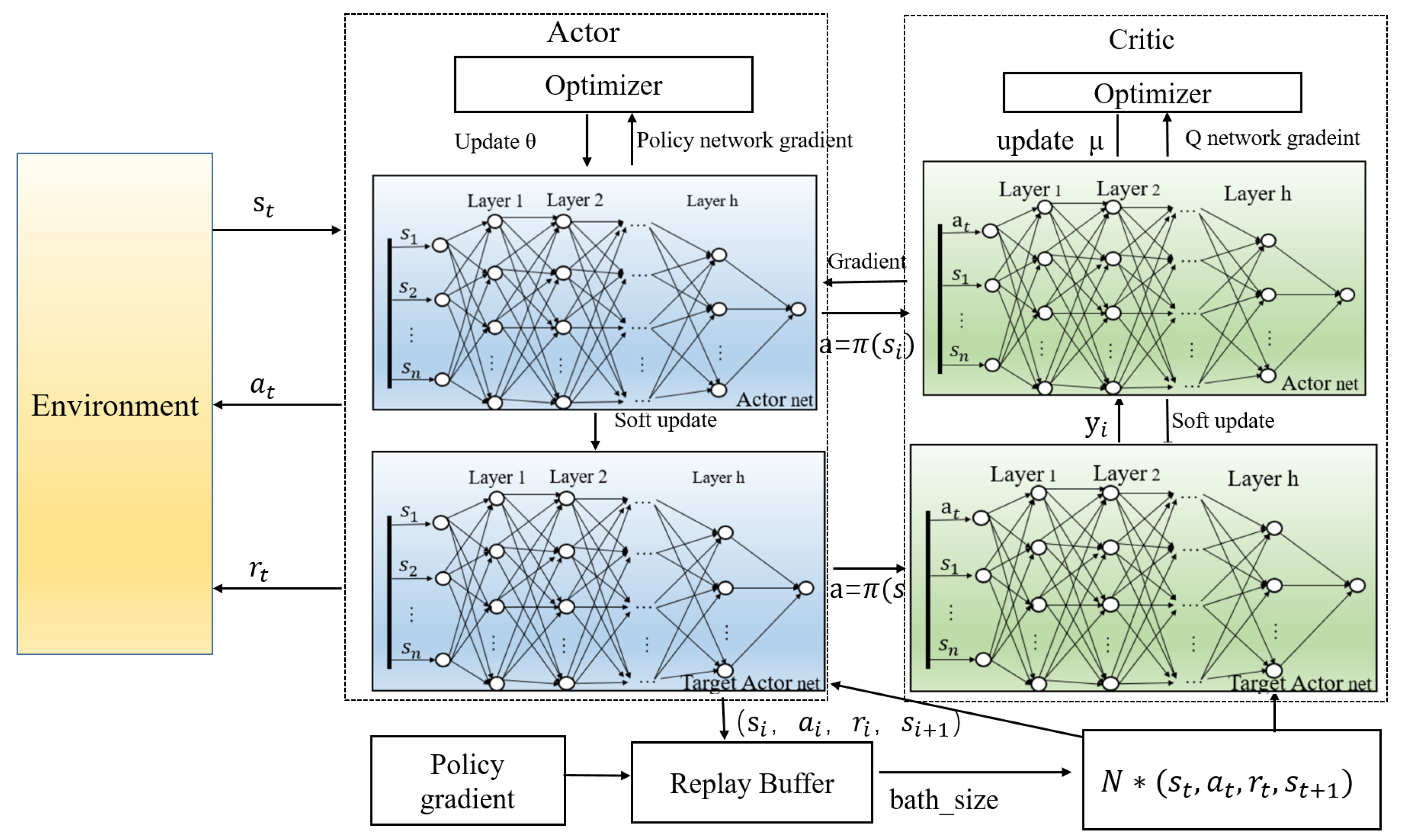
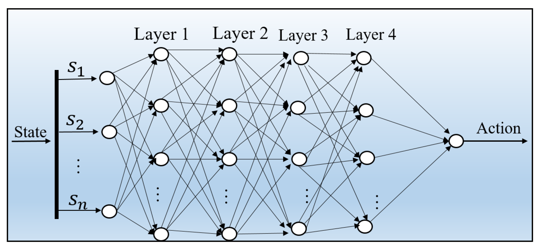
3.2.1. Agent Structure

In this paper, the Deep Deterministic Policy Gradient (DDPG) algorithm [26] is utilized to design the agent. The structure of the DDPG is schematically shown in Figure 5, which consists of a target network and a training network. Both networks belong to the Actor–Critic architecture, where the Actor computes the actions of the agent based on the state of the environment through a policy gradient and decides which actions to perform in the current state to obtain positive rewards. The Critic scores the actions performed by the agent and computes a value function based on the actions, which affects the probability distribution of the actions.
The DDPG contains four neural networks, namely, the Actor network, the Critic network, the Target Actor network, and the Target Critic network. The parameters of the Critic network are denoted by θ ω and the parameters of the Actor network are denoted by θ μ . The Actor network is used to output the action, and the Critic network is used to estimate the Q-value of the action, i.e., Q ( s , a | θ ω ) . After that, the Actor network calculates the gradient to adjust its action output strategy based on the Q value, updating the Actor’s network parameter θ μ . The Critic network is optimized by fitting the future target value based on the reward value and the Q value of the next step, i.e., Q . Then, the output of the Critic network is made to approximate the objective value. However, Q in the target value is a prediction value, so the target value is unstable. Therefore, the DDPG constructs the Target Actor network and the Target Critic network, respectively, where the Target Critic network calculates the Q in the target value, and the next action a needed by Q is output from the Target Actor network.
(1) Network structure
The Actor network structure is shown in Figure 6. For the Actor network, the network structure is determined as one input layer, four hidden layers, and one output layer, considering the variation of multiple variables. Among them, the input layer is used to receive state inputs and the intermediate layer is used to complete the mapping from state to action. We choose ReLU as the activation function. As argued in the literature [27], the Relu function can effectively improve the sparsity of the network and mitigate the overfitting problem. At the same time, it can effectively avoid the phenomenon of gradient vanishing. Considering that the controller output has to satisfy certain physical constraints, we refer to the research results from the literature [28] and adopt the tanh activation function in the output layer, whose smoothness and bounded output range of [−1, 1] can ensure that the generated control instructions are always within the physically realizable range.
The Critic network structure is shown in Figure 7. The Critic network is designed to evaluate the value of a particular action by outputting a Q-value function using the current state and the action as inputs. The Critic network consists of a state path and an action path. The state path is structured with one input layer, two hidden layers and one output layer to capture the relevant features of the input state. The action path is also designed with one input layer, three hidden layers, and one output layer, and the ReLu activation function is used to handle the high dimensional action information and the coupling relationship of each component.
(2) Hyper-parameters
Based on the network structure design described above, the key hyper-parameters of the network are shown in Table 2, which lists the settings of key network parameters in the DRL controller, including the number of hidden layers, the number of nodes in each layer, the learning rate, and the soft update rate for both the Actor network and the Critic network. In addition, the size of the Replay Buffer, the batch size, and the discount factor are specified.

3.2.2. Principles of Policy Optimization

The DDPG contains a total of four neural networks. The Target Actor network predicts the next action a = π ( s t + 1 | θ μ ) , and the Target Critic network can compute the target Q-value function given the current state Q s t + 1 , π ( s t + 1 | θ μ ) | θ ω , which in turn can obtain the target value as follows:
y i = r i + γ Q s t + 1 , π ( s t + 1 | θ μ ) | θ ω
The Critic network outputs the Q-value function of the state-action at the current moment Q s t , a t | θ ω , which is used to evaluate the current strategy as good or bad. The parameters of the Critic network are updated by minimizing the loss value (mean square error loss), defining the loss function when the Critic network is updated as follows:
L = 1 N i y i Q s t , a t | θ ω 2
where a i = π ( s i | θ μ ) . Using the Q-value of the Critic network, the Actor network updates the parameters by a gradient ascent method to maximize the expected reward. The gradient of the policy at the time of updating can be expressed as follows:
θ μ J ( θ μ ) = 1 N i θ μ π s t | θ μ a Q s t , a | θ ω | a = π ( s t )
For the update of the Target network parameters θ μ and θ ω , the DDPG slowly approximates the parameters of the current network through a soft update mechanism, thus stably following the changes of the training network.
θ ω τ ω + 1 τ θ ω
θ μ τ θ + 1 τ θ μ
The DDPG algorithm combines the features of value function-based and policy-based approaches, which allows deep reinforcement learning to deal with continuous action spaces with some exploration capabilities. Therefore the DDPG optimization process is shown in Algorithm  1.    
Algorithm 1: DDPG pseudocode
Aerospace 12 00424 i001

3.3. Algorithm Setup

(1) Observations
Considering the aerodynamic stabilization conditions as well as the intensity limitations during engine operation, eight quantities were selected as the engine state observation, y = [ n R H , n R L , S M C , S M f , T t 41 , δ n R L , δ π , δ π B ] T .
(2) Action space construction
The DRL controller replaces the w f , A 8 , and A 8 , o u t e r controllers in the PID controller, so the action space is represented as μ t = [ w f , A 8 , A 8 , o u t e r ] T .
The Action Space Pruning (ASP) method involved in the literature [29] is also used to customize the strategy for pruning. There are various ways to implement the Action Space Pruning strategy, such as the empirical formula method, polynomial fitting method, neural network fitting method, etc. In this paper, the neural network fitting method is chosen for the design of the Action Space Pruning strategy.
The PID controller data acquisition is carried out first. By carrying out large-scale simulation experiments under a variety of operating conditions, the altitude values, Mach numbers, throttle stick angles under different operating conditions, and the corresponding PID controller outputs of important controllable parameters such as fuel flow, nozzle area, and the target commands of the engine model are recorded. These data are organized into a structured dataset, which serves as the basis for subsequent neural network training.
These data were then fitted using a Backpropagation (BP) neural network to obtain a neural network that outputs controllable parameters based on the altitude, Mach number, and thrust commands, with specific neural network inputs and outputs as shown in Table 3.
Taking the output of the trained BP neural network as a benchmark, the action outputs obtained by the agent through the network computation are limited to ±30% of the benchmark value, thus reducing the range of exploration, increasing the convergence speed, and focusing more on effective strategies. As training progresses, the agent will make careful adjustments around the baseline values, thus improving the quality of the training data, reducing invalid or abnormal training data, and ensuring that the network better fits the target control strategy.
(3) Reward function setting
In the whole control system, the process of setting the reward function is equivalent to the process of formulating learning objectives for the agent. For the closed-loop control of the main combustion chamber fuel flow and nozzle throat area of the ITMA engine, the control objective is to minimize the error between the controlled variables and the target command by adjusting the input μ t = [ W f , A 8 , A 8 , o u t e r , w f , a f t e r , α C , A m i x ] of the aero-engine under different flight environments. At the same time, we ensure that the key performance parameters of the engine cannot exceed the limiting values in extreme operating environments. Therefore, the reward function is set as follows.
r 1 = 5 , δ n R L < 0.0001 0 , 0 δ n R L < 0.0003 1 , 0.0003 δ n R L < 0.0005 50 , 0.0005 δ n R L < 0.001 100 , δ n R L 0.01
The first part is the speed error reward function, which is designed as a stepwise reward function to achieve the target speed. The smaller the error, the larger the reward value.
r 2 = 2 , δ π < 0.001 0 , 0 δ π < 0.003 1 , 0.003 δ π < 0.005 50 , 0.005 δ π < 0.01 100 , δ π 0.01
r 3 = 2 , δ π B < 0.001 0 , 0 δ π B < 0.003 1 , 0.003 δ π B < 0.005 50 , 0.005 δ π B < 0.01 100 , δ π B 0.01
Similarly, the second and third parts are the error reward functions for the internal and external pressure ratios, respectively, which require lower tracking accuracy.
r 4 = i ω i max ( c i ( t ) c i , l ( t ) , 0 )
The total reward is given by the following:
r = r 1 + r 2 + r 3 + r 4
In the last section, c i ( t ) is the engine’s key performance parameter, which contains the engine speed, the surge margin, and the pre-turbine temperature. ω i is a constant representing the weight associated with each critical engine performance parameter in the reward function. Specifically, it is used to amplify negative rewards when critical performance parameters (such as engine speed, surge margin, or pre-turbine temperature) exceed the limits. ω i = 500 . When the critical performance parameters do not exceed the limit values, this section is zero and the control strategy is not affected. When one of the key performance parameters exceeds the limit, the environment generates a large negative reward so that the agent is influenced to avoid making actions that exceed the limit.

3.4. Network Training

3.4.1. Overall Training Framework and Data Interaction

The network training architecture is shown in Figure 8, which presents a complete picture of the overall training framework of the DRL control system and its key components. The operation of the engine control system during the network training process is divided into two phases. The first phase is the engine startup phase, and the first 30 s are designated as the engine startup phase in the mathematical simulation model. This phase is taken over by the conventional PID controller during the training process in order to eliminate the interference of the startup process on the DRL training. After successful startup, the control is handed over to the DRL system. After that, training is performed based on the DDPG algorithm as follows: the Actor network outputs the action, the Critic network estimates the Q-value of the action, the Target Critic network calculates the Q-value in the target value, and the Target actor network outputs the next desired action. In this process, the samples ( s t , a t , r t , s t + 1 ) obtained in the current step are put into the Replay Buffer. When the parameters are updated, N samples are randomly selected from the Replay Buffer to form a small batch of data, and the DDPG algorithm is strictly followed to update the network parameters. In addition, in order to increase the robustness of the network, we add a certain degree of random noise when outputting the action.
The engine model and the agent interact with each other through data to realize the single-step update of the agent network parameters as well as the training optimization mentioned in Section 3.2.2, and the specific interaction process is as follows:
Firstly, we initialize the network parameters of the agent, determine the flight environment of the engine, and obtain the target command by calculation. We start the engine and switch to the DRL controller after 30s. Through the target command and engine output, we calculate the state input of the agent s t , obtain the benchmark value through the ASP strategy, limit the action to within ±30% of the benchmark value, train to obtain the action output, input it into the ITMA engine model, calculate the state input of the agent in the next step s t + 1 , obtain the reward value r t through the pre-set reward function calculation module, and put the experience sample ( s t , a t , r t , s t + 1 ) obtained in the current step into the Replay Buffer. Finally, we update the network parameters, N samples are randomly sampled in small batches from the Replay Buffer, and the network parameters are updated according to the DDPG algorithm. The specific interaction table is shown in Table 4. In this training process, the training-related hyper-parameters are shown in Table 5.

3.4.2. Training Results and Analysis

Figure 9 shows a plot of the reward value versus the number of training epochs of the network. The horizontal axis of the graph represents the training epochs and the vertical axis shows the reward in 10 5 . From the graph, it can be seen that the training technique using ASP technology (red solid line) has a faster convergence rate compared to the base method (blue solid line). The following key conclusions can be drawn from the analysis: the pure DRL curve shows a slow upward trend and requires more training cycles to reach a steady state. The combined DRL + ASP curve exhibits a steeper upward slope in the early training phase, i.e., the ASP technique allows the system to reach the final performance level of pure DRL in about one-third of the training cycles.

4. Simulation Results and Analysis

Two typical working conditions—H = 0 km, Ma = 0; and H = 10 km, Ma = 0.9—are selected for the control system simulation test, and the results are as follows.

4.1. Simulation Results and Analysis for H = 0 km, Ma = 0

Figure 10 and Figure 11 show the PID control and DRL control simulation for H = 0 km, Ma = 0. Respectively, Figure (a) reflects the variation of the throttle stick, and Figures (b), (c), and (d) show the curve tracking of the low-pressure relative rotational speed, connotation drop ratio, and the outer boost ratio, respectively. Figures (e) and (f) show the variation of engine pre-turbine temperature, high-pressure compressor surge margin, and fan surge margin during the variation of the throttle stick according to (a).
Table 6 shows the response time and overshoot of the PLA under the PID and DRL methods during the process of change shown in Figure 10a. Based on the data in Table 6, the following conclusions can be drawn: the dynamic tracking effect of n R L is shown in Figure 10b and Figure 11b, respectively. In each acceleration and deceleration phase, the DRL controller can reduce the response time by an average of 43.65% while maintaining a comparable level of overshooting with PID (for most operating conditions). Figure 10c and Figure 11c show the control effect of the connotation drop ratio under two different controllers, respectively. Overall, the difference in response time between the DRL controller and the PID controller is small, but the DRL controller has an overall lower overshoot, especially during the rapid deceleration of the PLA from 30 to 20, which shows higher stability. The control effect of the outer boost ratio is shown in Figure 10d and Figure 11d. Overall, the response time of the DRL controller is generally shorter than that of the PID controller. In addition, (e) and (f) of Figure 10 and Figure 11 show the variation of T t 41 , SM, respectively, and the red dashed line in the figure indicates the maximum or minimum limit value of this parameter; both controllers are able to keep the engine in a safe operating condition during acceleration and deceleration.

4.2. Simulation Results and Analysis for H = 10 km, Ma = 0.9

Figure 12 and Figure 13, respectively, show the control renderings of PID control and DRL control under H = 10 km and Ma = 0.9 conditions.
From Figure 12c,d, it can be seen that under the environment of H = 10 km and Ma = 0.9, the target pressure ratio of the PLA remains unchanged above 65 deg, and the target relative speed of the engine starts to maintain a constant value after the PLA is above 90 deg in Figure 13a,b. As far as the data in the Table 7 are concerned, the actual values of the low-pressure relative speed and pressure ratio under the PID controller fluctuate significantly, with large increases or decreases several times, which deviate from the target values. The DRL controller can reduce the response time by an average of 45.34%, with relatively less fluctuations.

5. Conclusions

In this paper, a control method based on deep reinforcement learning (DRL) is innovatively proposed for a wide-range variable-cycle aero-engine with a turbine interstage mixed architecture (ITMA). By constructing a deep reinforcement learning control framework, it focuses on solving the control limitation problem of PID control under multi-variate coupling conditions. Two typical flight conditions (H = 0 km, Ma = 0 and H = 10 km, Ma = 0.9) are selected for the study to conduct digital simulation comparison experiments, and the results are discussed.
The proposed DRL control method breaks through the architectural single-input single-output (SISO) limitation of the traditional ITMA controller, and it effectively solves the strong coupling problem among multiple control variables through the feature extraction capability of deep neural networks. In terms of action space design, an innovative action space pruning method is adopted, which significantly reduces the ineffective exploration range of the agent, resulting in a significant increase in the convergence speed, at the same time ensuring the effectiveness of the strategy search.
The simulation data show that compared with the PID control, the DRL controller reduces the dynamic response time by an average of 44.5% while maintaining a similar amount of overshooting, especially in the transition state condition, which exhibits better dynamic tracking performance.
The fast response characteristics and stable control accuracy of this control method are particularly suitable for the control needs of high-mobility military aero-engines. This study provides a new technical route for the DRL control of aero-engines, and subsequent studies will focus on algorithm optimization, including (1) introducing migration learning to improve the control accuracy, (2) developing a lightweight network structure to improve the computational efficiency, and (3) expanding to more complex multi-task collaborative control scenarios in order to meet the needs of the future engineering applications of adaptive cyclic engines.

Author Contributions

Conceptualization, Y.D. and H.S.; methodology, Y.D., F.W. and Y.M.; software, Y.D.; validation, Y.D. and H.S.; formal analysis, Y.D.; investigation, H.S. and Y.D.; resources, H.S. and Y.D.; data curation, Y.D.; writing—original draft preparation, Y.D.; writing—review and editing, H.S. and Y.D.; visualization, Y.D.; supervision, H.S., F.W. and Y.M.; project administration, F.W., Y.M. and H.S.; funding acquisition, F.W., Y.M. and H.S. All authors have read and agreed to the published version of the manuscript.

Funding

This research received no external funding.

Institutional Review Board Statement

Not applicable.

Informed Consent Statement

Not applicable.

Data Availability Statement

Dataset available on request from the authors. The raw data supporting the conclusions of this article will be made available by the authors on request.

Conflicts of Interest

The authors declare no conflicts of interest.

Abbreviations

The following abbreviations are used in this manuscript:
VCEVariable Cycle Engine
ITMAInterstage Turbine Mixed Architecture
DDPGDeep Deterministic Policy Gradient
DRLDeep Reinforcement Learning

Appendix A

Table A1. Notation.
Table A1. Notation.
SymbolAdjustable Variable NameUnit
A 8 Nozzle throat area (inner) m 2
A 8 , o u t e r Nozzle throat area (outer) m 2
A m i x Internal and external bleed air intake area m 2
n L Fan physical speedr/min
n C H High-pressure corrected speedr/min
n R L Low-pressure relative speed\
n R H High-pressure relative speed\
P 0 Atmospheric static pressurePa
P t 2 Engine intake pressurePa
P s 31 Pressure after high-pressure compressorPa
P t 6 Post-turbine pressurePa
P t 16 Pre-combustor pressure (outer bypass)Pa
PLAThrottle lever angledeg
S M C Surge margin of high-pressure compressor\
S M F Surge margin of fan\
T t 2 Atmospheric static temperatureK
T t 25 Temperature after fanK
T t 41 Pre-turbine temperatureK
w f Main combustion chamber fuel flowkg/s
w f , a f t e r Afterburner fuel flowkg/s
α C Guide vane angle of the high-pressure compressordeg
π Pressure ratio\
BBypass ratio\
cmdTarget value\

References

  1. Huang, X.; Chen, Y.; Zhou, H. Analysis on development trend of global hypersonic technology. Bull. Chin. Acad. Sci. 2024, 39, 1106–1120. [Google Scholar]
  2. Zhong, S.; Kang, Y.; Li, X. Technology Development of Wide-Range Gas Turbine Engine. Aerosp. Power 2023, 4, 19–23. [Google Scholar]
  3. Johnson, L. Variable Cycle Engine Developments at General Electric-1955-1995; AIAA: Reston, VA, USA, 1995; pp. 105–143. [Google Scholar]
  4. Mu, Y.; Wang, F.; Zhu, D. Simulation of variable geometry characteristics of single bypass variable cycle engine. Aeroengine 2024, 50, 52–57. [Google Scholar]
  5. Brown, R. Integration of a variable cycle engine concept in a supersonic cruise aircraft. In Proceedings of the AIAA/SAE/ASME 14th Joint Propulsion Conference, Las Vegas, NV, USA, 18–20 June 1978. [Google Scholar]
  6. Allan, R. General Electric Company variable cycle engine technology demonstrator p-rogram. In Proceedings of the AIAA/SAE/ASME 15th Joint Propulsion Conference, Las Vegas, NV, USA, 18–20 June 1979. [Google Scholar]
  7. Feng, Z.; Mao, J.; Hu, D. Review on the development of adjusting mechanism invariable cycle engine and key technologies. Aeroengine 2023, 49, 18–26. [Google Scholar]
  8. Zhang, Y.; Yuan, W.; Zou, T. Modeling technology of high-flow triple-bypass variable cycle engine. J. Propuls. Technol. 2024, 45, 35–43. [Google Scholar]
  9. Liu, B.; Nie, L.; Liao, Z. Overall performance of interstage turbine mixed architecture variable cycle engine. J. Propuls. Technol. 2023, 44, 27–37. [Google Scholar]
  10. Zeng, X.; Gou, L.; Shen, Y. Analysis and modeling of variable cycle engine control system. In Proceedings of the 11th International Conference on Mechanical and Aerospace Engineering (ICMAE), Athens, Greece, 18–21 July 2020. [Google Scholar]
  11. Wu, Y.; Yu, Z.; Li, C.; He, M. Reinforcement learning in dualarm trajectory planning for a free-floating space robot. Aerosp. Sci. Technol. 2020, 98, 105657. [Google Scholar] [CrossRef]
  12. Gu, S.; Holly, E.; Lillicrap, T. Deep reinforcement learning for robotic manipulation with asynchronous off-policy updates. In Proceedings of the IEEE International Conference on Robotics & Automation, Singapore, 29 May–3 June 2017. [Google Scholar]
  13. Wada, D.; AraujoEstrada, S.A.; Windsor, S. Unmanned aerial vehicle pitch control under delay using deep reinforcement learning with continuous action in wind tunnel test. Aerospace 2021, 8, 258. [Google Scholar] [CrossRef]
  14. Liu, Y.; Liu, H.; Tian, Y. Reinforcement learning based two-level control framework of UAV swarm for cooperative persistent surveillance in an unknown urban area. Aerosp. Sci. Technol. 2020, 98, 261–281. [Google Scholar] [CrossRef]
  15. Sallab, A.; Abdou, M.; Perot, E. End-to-End deep reinforcement learning for lane keeping assist. In Proceedings of the 30th Conference on Neural Information Processing Systems (NIPS), Barcelona, Spain, 5–10 December 2016. [Google Scholar]
  16. Kiran, B.; Sobh, I.; Talpaert, V. Deep reinforcement learning for autonomous driving: A survey. IEEE Trans. Intell. Transp. Syst. 2021, 28, 4909–4926. [Google Scholar] [CrossRef]
  17. Mehryar, M.; Afshin, R.; Talwalkar, A. Reinforcement learning. In Foundations of Machine Learning; MIT Press: Cambridge, MA, USA, 2018; pp. 379–405. [Google Scholar]
  18. Mnih, V.; Kavukcuoglu, K.; Silver, D. Playing Atari with deep reinforcement learning. arXiv 2013, arXiv:1312.5602. [Google Scholar]
  19. Qiu, X. Deep Reinforcement Learning. In Foundations of Machine Learning; China Machine Press: Beijing, China, 2020; pp. 339–360. [Google Scholar]
  20. Francois-Lavet, V.; Henderson, P.; Islam, R. An introduction to deep reinforcement learning. Found. Trends Mach. Learn. 2018, 11, 219–354. [Google Scholar] [CrossRef]
  21. Zheng, Q.; Jin, C.; Hu, Z. A study of aero-engine control method based on deep reinforcement learning. IEEE Access 2018, 6, 67884–67893. [Google Scholar] [CrossRef]
  22. Liu, C.; Dong, C.; Zhou, Z. Barrier Lyapunov function based reinforcement learning control for air-breathing hypersonic vehicle with variable geometry inlet. Aerosp. Sci. Technol. 2020, 96, 105537–105557. [Google Scholar] [CrossRef]
  23. Fang, J.; Zheng, Q.; Cai, C. Deep reinforcement learning method for turbofan engine acceleration optimization problem within full flight envelope. Aerosp. Sci. Technol. 2023, 136, 108228–108242. [Google Scholar] [CrossRef]
  24. Tao, B.; Yang, L.; Wu, D. Deep reinforcement learning-based optimal control of variable cycle engine performance. In Proceedings of the 2022 International Conference on Advanced Robotics and Mechatronics (ICARM), Guilin, China, 7–9 November 2022. [Google Scholar]
  25. Gao, W.; Zhou, X.; Pan, M. Acceleration control strategy for aero-engines based on model-free deep reinforcement learning method. Aerosp. Sci. Technol. 2022, 120, 107248–107260. [Google Scholar] [CrossRef]
  26. Silver, D.; Lever, G.; Heess, N. Deterministic Policy Gradient Algorithms. Proc. Mach. Learn. Res. 2014, 32, 387–395. [Google Scholar]
  27. Hahnloser, R.; Sarpeshkar, R.; Mahowald, M. Digital selection and analogue amplification coexist in a cortex-inspired silicon circuit. Nature 2000, 405, 947–951. [Google Scholar] [CrossRef] [PubMed]
  28. He, K.; Zhang, X.; Ren, S.; Sun, J. Delving deep into rectifiers: Surpassing human-level performance on ImageNet classification. In Proceedings of the IEEE International Conference on Computer Vision (ICCV), Santiago, Chile, 7–13 December 2015. [Google Scholar]
  29. Kanervisto, A.; Scheller, C.; Hautamäki, V. Action space shaping in deep reinforcement learning. In Proceedings of the 2020 IEEE Conference on Games (CoG), Osaka, Japan, 24–27 August 2020. [Google Scholar]
Figure 1. Schematic diagram of the engine structure.
Aerospace 12 00424 g001
Figure 2. Reinforcement learning schematic.
Aerospace 12 00424 g002
Figure 3. Structure of the ITMA controller.
Aerospace 12 00424 g003
Figure 4. Control law diagram of α C and A m i x : (a) describes the plot of α C as a function of n C H . (b) shows the plot of A m i x as a function of Ma.
Aerospace 12 00424 g004
Figure 5. Structure of the DDPG algorithm.
Aerospace 12 00424 g005
Figure 6. Actor network structure.
Aerospace 12 00424 g006
Figure 7. Critic network structure.
Aerospace 12 00424 g007
Figure 8. Network training structure diagram.
Aerospace 12 00424 g008
Figure 9. Training progress curve.
Aerospace 12 00424 g009
Figure 10. PID control simulation for H = 0 km, Ma = 0: (a) describes the variation of the throttle stick; (b) shows the curve tracking of the low-pressure relative rotational speed; (c) describes the curve tracking of connotation drop ratio; (d) shows the curve tracking of the outer boost ratio; and (e,f) show the variation of engine pre-turbine temperature high-pressure compressor surge margin, and fan surge margin during the variation of the throttle stick according to (a).
Aerospace 12 00424 g010
Figure 11. DRL control simulation for H = 0 km , Ma = 0 : (a) illustrates the variation of the throttle stick; (b) shows the curve tracking of the low-pressure relative rotational speed; (c) illustrates the curve tracking of the connotation drop ratio; (d) shows the curve tracking of the outer boost ratio; and (e,f) illustrate the variation of engine pre-turbine temperature, high-pressure compressor surge margin, and fan surge margin during the variation of the throttle stick as described in (a).
Aerospace 12 00424 g011
Figure 12. PID control simulation results at H = 10 km and M a = 0.9 : (a) shows the throttle lever angle variation; (b) demonstrates the low-pressure relative rotational speed tracking performance; (c) displays the connotation drop ratio tracking; (d) illustrates the outer culvert boost ratio tracking performance; and (e,f) present the variations of the engine pre-turbine temperature, high-pressure compressor surge margin, and fan surge margin during the throttle lever angle changes corresponding to (a).
Aerospace 12 00424 g012
Figure 13. DRL control simulation for H = 10 km and Ma = 0.9: (a) illustrates the variation of the throttle stick; (b) shows the curve tracking of the low-pressure relative rotational speed; (c) illustrates the curve tracking of the connotation drop ratio; (d) shows the curve tracking of the outer boost ratio; and (e,f) illustrate the variation of engine pre-turbine temperature, high-pressure compressor surge margin, and fan surge margin during the variation of the throttle stick as described in (a).
Aerospace 12 00424 g013
Table 1. Range of variable components.
NotationDefinitionRange
w f Main combustion chamber fuel flow0–1.4 (kg/s)
w f , a f t e r Afterburner fuel flow0–6 (kg/s)
α C Guide vane angle of the high-pressure compressor0–40 (deg)
A 8 Nozzle throat area0–0.45 ( m 2 )
A 8 , o u t e r Bypass nozzle throat area0–0.3 ( m 2 )
A m i x Internal and external bleed air intake area0–0.05 ( m 2 )
Table 2. Hyper-parameters.
ParameterValue
Number of hidden layers in the Actor network4
Number of hidden layers in the Critic networkState: 2, Action: 3
Number of nodes in the Actor network30, 30, 20, 20
Number of nodes in the Critic networkState: 30, 20, Action: 20, 20, 20
Learning rate of the Actor0.0001
Learning rate of the Critic0.001
Soft update rate0.001
Replay Buffer1,000,000
Number of samples in the replay Buffer N512
Discount factor γ 0.99
Table 3. BP network input and output.
NotationParameter NameUnitInput/Output
HFlight altitudekmInput
MaFlight Mach number\
n R L , c m d Low-pressure relative rotational speed command\
π c m d Connotation drop ratio command\
π B , c m d Outer culvert boost ratio command\
w f Main combustion chamber fuel flowkg/sOutput
A 8 Nozzle throat area m 2
A 8 , o u t e r Bypass nozzle throat area m 2
Table 4. Data interaction.
NotationInstructionsData
α C Open-loop control strategy agent model
w f DRL control strategy
w f Open-loop control strategy
A 8 DRL control strategy
A 8 , outer DRL control strategy
A mix Open-loop control strategy
P t 6 Calculate pressure ratio model agent
P s 31 Calculate pressure ratio and safety constraints
n RL For safety constraints
n RH For safety constraints
T t 41 For safety constraints
Table 5. Training-related parameters.
Parameter NameParameter Value
Dimensionality of observations8
Dimensionality of actions3
Training step0.02 s
Number of training epochs1000
Table 6. Comparative data for n R L , π , and π B at H = 0 km and M a = 0 .
Control TypePLAt/s (PID)Overshoot (PID)t/s (DRL)Overshoot (DRL) Δ t (%)
n R L 20–303.1641.4221.3741.7456.57
30–403.2600.5321.439055.86
40–502.58901.145055.77
50–602.20501.068051.56
60–502.10901.3140.837.70
50–402.20501.2320.244.13
40–301.91801.232035.77
30–208.2454.255.1392.2537.67
π 20–303.1479.191.7469.7644.64
30–402.49301.234050.54
40–502.30101.204047.87
50–602.20501.001054.58
60–502.58901.356047.72
50–402.68501.247053.66
40–302.87601.332053.75
30–203.87501.562059.67
π B 20–303.9310.26232.3360.301640.56
30–404.0270.6142.5980.67835.43
40–503.45202.356031.8
50–602.58902.33109.97
60–503.35602.547024.1
50–403.2602.368027.39
40–305.46502.896047.13
30–206.1360.3483.0190.25650.76
Table 7. Comparative data for n R L , π , and π B at H = 10 km and M a = 0.9 .
Control TypePLAt/s (PID)Overshoot (PID)t/s (DRL)Overshoot (DRL) Δ t (%)
n R L 60–753.1640.3441.5150.222552.04
75–604.0440.2071.6930.156358.19
60–902.8691.4291.837035.97
90–1153.451.2252.872016.75
π 60–752.8764.8010.8422.20535.96
75–602.7804.8451.3042.10653.03
60–903.9318.2521.8685.87452.43
90–1153.5475.6671.6583.26553.22
π B 60–752.3014.67091.0563.35654.06
75–603.1325.25161.7543.38643.99
60–903.06811.771.3988.9354.41
90–1153.3564.152.2092.2534.18
Disclaimer/Publisher’s Note: The statements, opinions and data contained in all publications are solely those of the individual author(s) and contributor(s) and not of MDPI and/or the editor(s). MDPI and/or the editor(s) disclaim responsibility for any injury to people or property resulting from any ideas, methods, instructions or products referred to in the content.

