ELVO-Based Autonomous Satellite Collision Avoidance with Multiple Debris

Abstract

The frequent occurrence of space debris collision incidents has made research on autonomous satellite avoidance necessary. Against this backdrop, the paper presents a short-term autonomous space debris avoidance algorithm based on the Equivalent Linear Velocity Obstacle (ELVO) paradigm, which addresses the challenges of multiple debris scenarios and real-time decision-making. Error analysis and compensating terms are provided to enhance the algorithm’s accuracy. Simulations are proposed to validate the algorithm, and the simplified design reduces the online computational load, demonstrating its feasibility for future on-orbit usage.

1. Introduction

In the last few decades, the amount of space debris has dramatically increased [1,2,3], and this trend is expected to continue in the near future. According to estimations by the European Space Agency, as of December 2023, the amount of space debris pieces exceeding 10 cm stands at approximately 36,500, with a staggering one million pieces ranging from 1 to 10 cm. With the continuous increase in satellites and space debris, the risk of collision has proliferated. When the density of objects in low Earth orbit (LEO) becomes too high, collisions between objects could trigger a cascade of further collisions, a phenomenon known as Kessler syndrome [4]. The collision of Kosmos 2251 with Iridium 33 in 2009 serves as a prime example.

Traditional collision avoidance maneuvers rely on ground station and manual operation, requiring extra time and computational resources. Decisions often have to be made days in advance, imposing substantial operational control burdens and increasing the likelihood of a high false-alarm rate. Given the continuous deterioration of the LEO environment, autonomous satellite avoidance is imperative.

Autonomous avoidance brings noteworthy merits. Satellite-borne sensors exhibit superior accuracy in close-range detection, thereby reducing observational uncertainties. Theses sensors for orbital debris detection include optical imagers, LiDAR, radar systems such as Synthetic Aperture Radar (SAR), and infrared detectors, with detection ranges spanning from a few meters to several hundred kilometers (e.g., refs. [5,6]). Optical sensors typically detect debris larger than 10 cm within 10–50 km under sufficient illumination. LiDAR enables high-precision detection of centimeter-scale objects at distances of 10 m to a few kilometers. Radar can detect debris over 10 cm in size at ranges exceeding 100 km, while infrared sensors are capable of identifying thermally contrasting objects at distances up to approximately 100 km. Detection capability is influenced by object size, material properties, and observational conditions. Recent studies on star tracker-based debris detection, such as [7,8], further validate this approach for space domain awareness. High-precision measurements can substantially mitigate false alarms, minimize unnecessary orbital maneuvers, and enable precise estimation of smaller safety margins. Furthermore, satellite-based sensors are capable of detecting uncatalogued space debris in close proximity that ground-based sensing systems cannot observe. By implementing emergency autonomous avoidance maneuvers, satellites are equipped with the capability to effectively respond to unexpected contingencies.

However, current autonomous avoidance systems face critical challenges, with the core contradiction lying in the mismatch between limited onboard resources and the dynamic demands of complex space environments. Specific challenges include the following:

• Severely constrained computational resources conflict sharply with high real-time responsiveness requirements for collision avoidance algorithms.
• Precious propellant and energy reserves necessitate minimizing frequent maneuvers, as they significantly shorten operational lifespans. Optimal orbital maneuvers must balance collision avoidance, propellant conservation, energy consumption, and mission continuity. (The term “balance” refers to the need to find an optimal trade-off between multiple objectives during orbital maneuvers. In general, these objectives may conflict with each other, meaning that prioritizing one goal could negatively impact others).
• Cascading collision risks emerge in constellation satellite clusters or densely populated orbital regions. A single collision avoidance maneuver may trigger domino-like collision chains, creating a situation that is exceptionally difficult to resolve. Indeed, mitigating global collision risks should be a priority and requires a systematic approach.

Scholars have recognized the aforementioned issues and devoted efforts to related research. A genetic algorithm based multiple debris avoidance method was proposed by [9], focusing on finding a safe orbit. Recently, Ref. [10] proposed an autonomous collision-avoidance strategy based on adaptive potential fields and [11] attempted to address the autonomous collision avoidance problem using a reinforcement learning approach. Regarding the mission level, Ref. [12] developed an autonomous spacecraft avoidance framework that dynamically coordinates routine operations and collision evasion through closed-loop planning. Beyond theoretical explorations, mission scenarios such as rendezvous, docking, and on-orbit servicing have been widely emulated on-ground in various facilities [13,14,15]. In particular, facilities such as the Test Environment for Applications of Multiple Spacecraft (TEAMS) and the Distributed Space Systems Laboratory (DSSL) provide experimental testbeds where collision avoidance algorithms have been successfully validated [16].

Nevertheless, real-time decision-making in multi-debris environments remains insufficiently resolved, particularly due to the computational complexity and dynamic uncertainties involved. Furthermore, existing approaches typically focus on avoidance at a single point in time, neglecting the spacecraft’s entire trajectory. This oversight may compromise the satellite’s long-term safety.

In this paper, we propose an algorithm for short-term autonomous avoidance of multiple debris, leveraging the Equivalent Linear Velocity Obstacle (ELVO) method, which is inspired by the Velocity Obstacle concept introduced by [17]. VO paradigm is one effective method for addressing the challenge of autonomous navigation for robots and vehicles [18], which was later improved into multi-agent cases by [19,20]. Robotic experiments [21,22] have shown that VO-based obstacle avoidance methods perform well, demonstrating their effectiveness and reliability in dynamic environments. While the original VO paradigm focused on uniform linear motion with impulse control, several variations have been proposed to extend its application scenarios. Ref. [23] proposed ELVO, extending VO to arbitrary trajectories by considering equivalent linear trajectories of objects, while [20] studied robots with finite acceleration, and [24,25] applied the method to 3D scenarios.

By dynamically computing the Velocity Obstacle Domain (VOD) between debris and the spacecraft, we can generate avoidance paths in real time, making the approach suitable for multi-debris scenarios. It should be noted that this method is valid only under the assumptions of linear uniform motion, impulsive control, and accurate measurement. So, it leads to certain safety risks for satellites during actual close-range space avoidance maneuvers. We overcome the aforementioned issues through safety distance compensation and adaptive online adjustment. This approach demonstrates that, as long as the maneuverability can satisfy the velocity increment required by the ELVO method, the algorithm guarantees collision-free operation for the satellite in short-term scenarios. Detailed error analysis is provided. Finally, we integrate the proposed autonomous algorithm into a traditional long-term avoidance system, and discuss under what circumstances it is appropriate to activate this algorithm for short-term autonomous avoidance.

The rest of this paper is organized as follows. Section 2 outlines the problem formulation and Section 3 develops an ELVO-based collision avoidance algorithm supported by error analysis. This algorithm is integrated into long-term avoidance strategies and discussed in Section 4. Section 5 evaluates the method through numerical simulations of two scenarios, while Section 6 concludes the work.

2. Problem Formulation

This paper studies autonomous collision avoidance of a satellite against multiple proximate space debris objects. Assume that multiple pieces of space debris are distributed near the satellite’s mission orbit, and all of them are within the observable range of the satellite’s onboard sensors. At time $t=t_0$, the satellite has received warnings indicating that some of them are predicted to collide with it at specific future moments. More precisely, let the Time of Closest Approach (TCA) between the satellite and the space debris be denoted as ${\overline{t}}_C^i,i=1,\cdots n_d$, where $n_d$ is the number of the proximate debris. We say that debris i collides with the satellite, if their distance at time ${\overline{t}}_C^i$ is less than or equal to the preset safety distance $R^i$. To avoid collisions, the satellite will execute an autonomous orbital maneuver, which needs to meet the following engineering constraints:

• Control saturation;
• Fuel efficiency;
• Mission continuity.

2.1. Coordinate System

In this work, the Local Vertical Local Horizontal (LVLH) coordinate system is employed to analyze the satellite and debris dynamics, as follows:

• Introduce a reference orbit, whose orbital elements are consistent with those of the satellite at time $t=0$ before any maneuver is performed. The semi-major axis, eccentricity, inclination, right ascension of the ascending node, argument of periapsis, and true anomaly of the reference orbit are denoted by

  $$a_{ref},e_{ref},i_{ref},{\Omega }_{ref},{\omega }_{ref},{\varphi }_{ref}.$$
• The origin of the LVLH coordinate system is located at the center of mass of the reference satellite. The x-axis points from the center of the Earth to the satellite’s center of mass (local vertical), the z-axis points in the direction of the orbital angular momentum vector (perpendicular to the orbital plane), and the y-axis completes the right-handed coordinate system by pointing in the direction of the satellite’s velocity vector (local horizontal).

2.2. Dynamics Models

This paper employs a time-variant linear model from [26] to describe the relative motion with respect to the elliptical reference orbit. In the LVLH coordinate system, the relative motion of the space debris can be written as a series of time-varying linear equations:

$${\dot{\mathit{x}}}^i\left(t\right)=\mathit{A}\left(t\right){\mathit{x}}^i\left(t\right),i=1,\cdots n_d,$$

(1)

where ${\mathit{x}}^i={({\mathit{r}}^{i\top },{\mathit{v}}^{i\top })}^{\top }$ denotes the state of the i-th debris, which consists of both position and velocity components. Moreover, matrix $\mathit{A}\left(t\right)$ is defined by

$$\mathit{A}\left(t\right)=\left(\begin{array}{cccccc}0& 0& 0& 1& 0& 0\\ 0& 0& 0& 0& 1& 0\\ 0& 0& 0& 0& 0& 1\\ ine{n}_{ref}^2+2{\displaystyle \frac{\mu }{r_{ref}^3}}& -{ϵ}_{ref}& 0& 0& 2n_{ref}& 0\\ {ϵ}_{ref}& n_{ref}^2-{\displaystyle \frac{\mu }{r_{ref}^3}}& 0& -2n_{ref}& 0& 0\\ 0& 0& -{\displaystyle \frac{\mu }{r_{ref}^3}}& 0& 0& 0\end{array}\right),$$

(2)

where $\mu$ is the Earth gravity constant, and

$$\left\{\begin{array}{cc}\hfill r_{ref}& ={\displaystyle \frac{a_{ref}(1-e_{ref}^2)}{1+e_{ref}cos{\varphi }_{ref}}}\hfill \\ \hfill n_{ref}& =\sqrt{{\displaystyle \frac{\mu (1+e_{ref}cos{\varphi }_{ref})}{r_{ref}^3}}}\hfill \\ \hfill {ϵ}_{ref}& =-{\displaystyle \frac{2\mu e_{ref}sin{\varphi }_{ref}}{r_{ref}^3}}\hfill \end{array}\right.$$

are the time-varying terms depending on the orbital elements of the reference satellite. Clearly, if $e_{ref}\equiv 0$, Equations (1) and (2) become time-invariant, which are the well-known Clohessy–Wiltshire (C-W) equations.

Similarly, in the LVLH coordinate system, the dynamics for the satellite are

$${\dot{\mathit{x}}}^0\left(t\right)=\mathit{A}\left(t\right){\mathit{x}}^0\left(t\right)+\mathit{B}\mathit{u}\left(t\right),$$

(3)

where ${\mathit{x}}^0={({\mathit{r}}^{0\top },{\mathit{v}}^{0\top })}^{\top }$ denotes the state of the satellite and $\mathit{B}={\left({\mathit{O}}_{3\times 3},{\mathit{I}}_{3\times 3}\right)}^{\top }$ is the control matrix, with $\mathit{O}$ and $\mathit{I}$ being the zero and identity matrices of corresponding shapes. The control input $\mathit{u}$, which represents the satellite’s orbital thrust acceleration, is bounded by its maximum value $u_{max}$.

3. Elvo-Based Space Debris Avoidance

Write the relative state between the satellite and the i-th debris as

$${\mathit{x}}^{0i}\left(t\right)={\mathit{x}}^0\left(t\right)-{\mathit{x}}^i\left(t\right),i=1,\cdots n_d.$$

Accordingly, the position and velocity components of ${\mathit{x}}^{0i}\left(t\right)$ are denoted by ${\mathit{r}}^{0i}\left(t\right)$ and ${\mathit{v}}^{0i}\left(t\right)$, respectively. In this section, we will design a fast online algorithm to ensure that the satellite maintains a safe distance from any space debris, i.e.,

$$∥{\mathit{r}}^{0i}\left(t\right)∥\ge R^i,\forall i=1,\cdots ,n_d,\forall t\ge t_0.$$

(4)

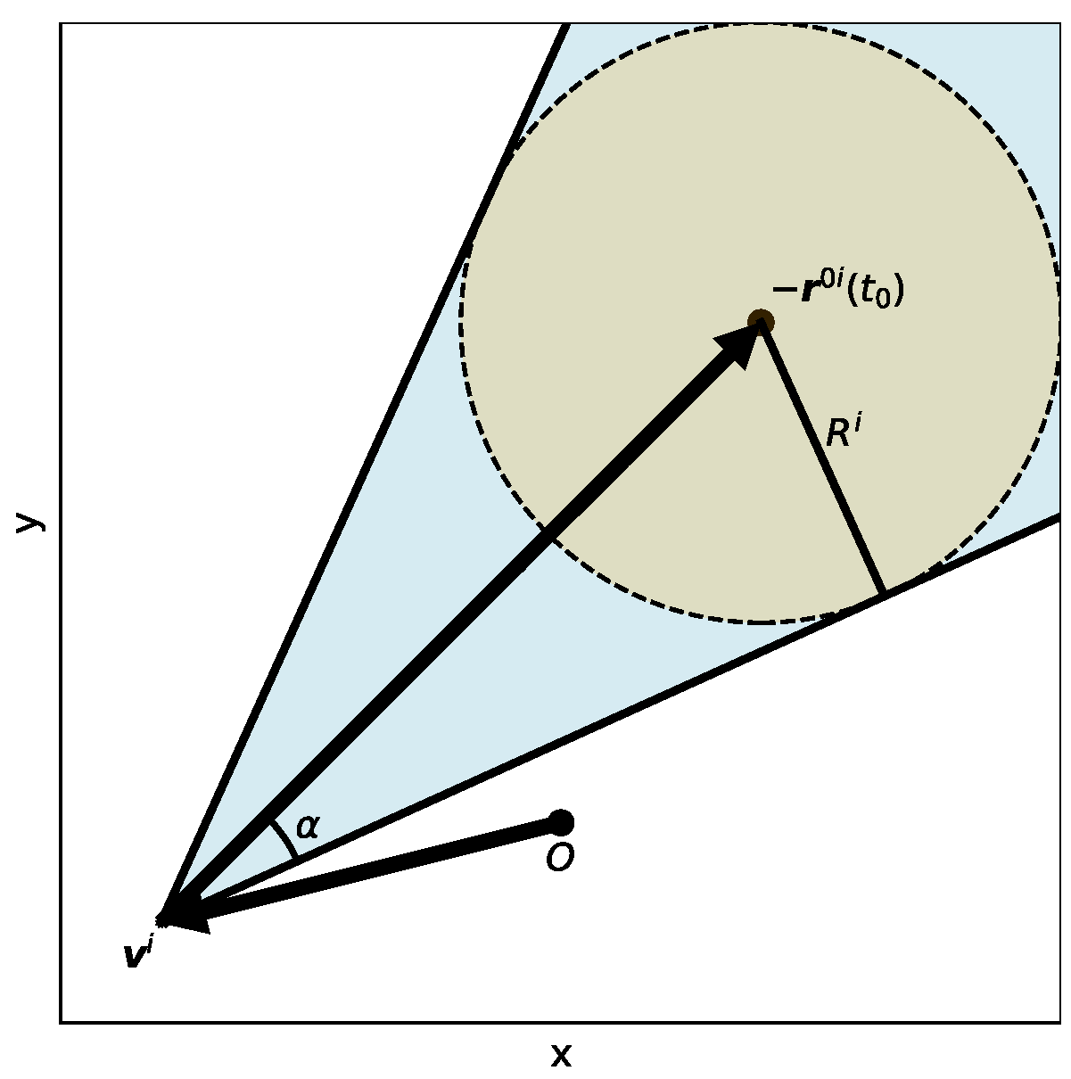
3.1. Velocity Obstacle

The Velocity Obstacle (VO) method is a geometric approach that defines the set of all velocities leading to collisions with other objects, under the assumption that these objects maintain their current velocities. In this work, the idea of VO is employed for space debris avoidance, and the errors introduced by the uniform linear motion assumption will be systematically analyzed and compensated.

We first elaborate on the fundamental principle of the VO method. To this end, we make an ideal assumption here, which will be relaxed in subsequent sections. Suppose the satellite with state ${\mathit{x}}^0$ performs an orbital maneuver control at time $t_0$ to avoid the debris with state ${\mathit{x}}^i$, where both objects are assumed to be in uniform linear motion (it holds when $[t_0,{\overline{t}}_C^i]$ is an extremely short time interval). Therefore, the relative position ${\mathit{r}}^{0i}\left(t\right)$ as a function of time and constant relative velocity ${\mathit{v}}^{0i}$ is given by the following equation:

$${\mathit{r}}^{0i}\left(t\right)={\mathit{r}}^{0i}\left(t_0\right)+t{\mathit{v}}^{0i}.$$

(5)

According to (5), the Relative Collision Cone for the satellite and the i-th debris is defined as the set of all relative velocities that lead to collision:

$$C{C}^{0i}:=\left\{{\mathit{v}}^{0i}|\underset{t\ge t_0}{min}{r}^{0i}\left(t\right)\le R^i\right\},$$

(6)

where $r^{0i}\left(t\right)$ is the magnitude of vector ${\mathit{r}}^{0i}\left(t\right)$. In the following, we denote the magnitude of vector $\mathit{a}$ by a without further explicit mention. Given the geometric relationship, it follows that $C{C}^{0i}$ forms a cone in the space of relative velocity, with apex, axis, and vertex angle defined by $\mathbf{0}$, $-{\mathit{r}}^{0i}\left(t_0\right)$ and $2arcsin(R^i/r^{0i}\left(t_0\right))$, respectively. Defining

$$\alpha :=arcsin(R^i/r^{0i}\left(t_0\right))$$

as the half-vertex angle of the cone, one obtains

$$C{C}^{0i}=\left\{{\mathit{v}}^{0i}|\angle \langle {\mathit{v}}^{0i},-{\mathit{r}}^{0i}\left(t_0\right)\rangle <\alpha \right\}.$$

(7)

The corresponding Velocity Obstacle is then the collection of all the velocities of the satellite that would result in a collision with the i-th debris:

$$\begin{array}{cc}\hfill V{O}^{0i}& :=C{C}^{0i}+{\mathit{v}}^i\hfill \\ \hfill & =\left\{{\mathit{v}}^0|\angle \langle {\mathit{v}}^{0i},-{\mathit{r}}^{0i}\left(t_0\right)\rangle <\alpha \right\}.\hfill \end{array}$$

(8)

Here, ${\mathit{v}}^0$ in (8) represents the satellite’s absolute velocity, whereas ${\mathit{v}}^{0i}$ in (6) denotes the relative velocity between the satellite and the i-th debris. This distinction in notation is intentional, aiming to highlight the transition from relative to absolute velocity space. Figure 1 illustrates the VO for the satellite and debris.

A velocity ${\mathit{v}}^0$ is collision-free for the satellite with respect to the i-th debris if and only if

$${\mathit{v}}^0\notin V{O}^{0i}.$$

Alternatively, this constraint can be expressed in terms of cosine as

$$cos\angle \langle {\mathit{v}}^{0i},-{\mathit{r}}^{0i}\left(t_0\right)\rangle \le cos\alpha ,$$

or, equivalently,

$$-{\displaystyle \frac{{\mathit{v}}^{0i}·{\mathit{r}}^{0i}\left(t_0\right)}{v^{0i}·r^{0i}\left(t_0\right)}}\le \sqrt{1-{\displaystyle \frac{{\left(R^i\right)}^2}{{\left(r^{0i}\left(t_0\right)\right)}^2}}}.$$

Considering all the space debris, we say a velocity ${\mathit{v}}^0$ is collision-free for the satellite if and only if

$$\begin{array}{c}\hfill {\mathit{v}}^0\notin \bigcup _{i}V{O}^{0i}.\end{array}$$

3.2. Equivalent Linear Velocity Obstacle

In view of (1) and (3), the satellite and debris typically undergo nonlinear motion in the LVLH coordinate system. So, these space objects with time-varying velocities ${\mathit{v}}^j\left(t\right),j=0,1,\dots ,n_d$, actually correspond to the positions

$${\mathit{r}}^j\left(t\right)={\mathit{r}}^j\left(t_0\right)+{\int }_{t_0}^t{\mathit{v}}^i\left(s\right)\mathrm{d}s.$$

In this sense, we apply the Equivalent Linear Velocity Obstacle (ELVO) method proposed by [23], defined below, which is a variation of VO developed to account for arbitrary trajectories.

Definition 1. 

The Equivalent Linear Velocity Obstacle (ELVO) between the satellite and the i-th debris at time $t_1$, denoted $ELV{O}^{0i}(t_1,t_0)$, is defined as the VO between the satellite and a virtual object which reaches ${\mathit{r}}^i\left(t_1\right)$ by moving at a constant velocity ${\mathit{v}}^j\left(t_1\right)$ over the interval $[t_0,t_1]$.

Evidently, the virtual object in Definition 1 has a constant velocity ${\mathit{v}}^i\left(t_1\right)$, and at any time t, its position satisfies

$${\widehat{\mathit{r}}}^i\left(t\right)={\mathit{r}}^i\left(t_1\right)+(t-t_1){\mathit{v}}^i\left(t_1\right),$$

as illustrated in Figure 2. So, $ELV{O}^{0i}(t_1,t_0)$ is defined as the VO between the satellite and this virtual object. That is,

$$ELV{O}^{0i}(t_1,t_0)=\left\{{\widehat{\mathit{v}}}^0|\angle \langle {\widehat{\mathit{v}}}^{0i},-{\widehat{\mathit{r}}}^{0i}\left(t_0\right)\rangle <\widehat{\alpha }\right\},$$

where ${\widehat{\mathit{r}}}^{0i}\left(t_0\right):={\mathit{r}}^0\left(t_0\right)-{\widehat{\mathit{r}}}^i\left(t_0\right)$, ${\widehat{\mathit{v}}}^{0i}:={\widehat{\mathit{v}}}^0-{\mathit{v}}^i\left(t_1\right)$ and $\widehat{\alpha }:=arcsin(R^i/\parallel {\widehat{\mathit{r}}}^{0i}\left(t_0\right)\parallel )$. Note that both ${\widehat{\mathit{v}}}^0$ and ${\widehat{\mathit{v}}}^{0i}$ are constant vectors, where ${\widehat{\mathit{v}}}^0$ represents a target velocity of the satellite.

It can be seen from Figure 2 that a portion of collisions resulting from a curved trajectory can be captured by the ELVO. The effectiveness of the method increases as the actual trajectory approaches a straight line. In fact, the velocity increment $\delta \mathit{v}$ provided above guarantees safety only under the assumptions of linear uniform motion, impulsive control, and accurate measurement. But in real close-proximity scenarios, these assumptions are not strictly valid, leading to potential safety risks. To ensure the effectiveness of the method, we need a larger safety distance ${\widehat{R}}^i$ to replace $R^i$ in (6). The specific value of ${\widehat{R}}^i$ will be calculated in the following section.

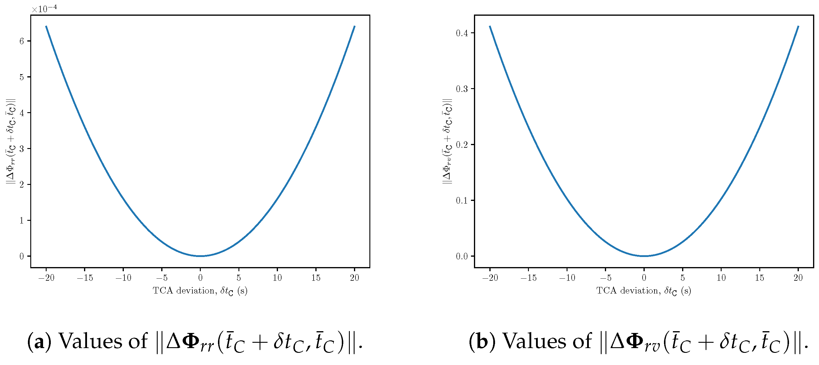
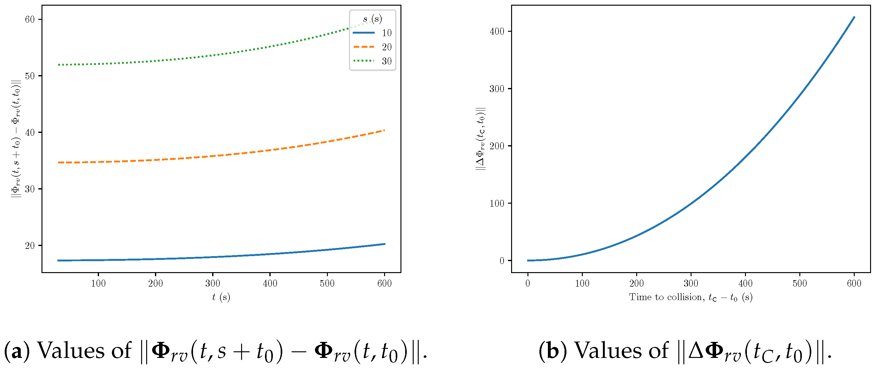
3.3. Compensated Safe Distance ${\widehat{R}}^i$

Determining ${\widehat{R}}^i$ in the ELVO method is crucial for satellite safety during the avoidance maneuvers. To compensate for the mentioned errors and maintain the required safety margins, additional terms must be added to the original safe distance $R^i$. Now, we will propose a compensated safe distance ${\widehat{R}}^i$ to substitute $R^i$ in (6) to guarantee a successful evasion.

Let $t_C^i:={\overline{t}}_C^i+\delta t_C^i$ be the new TCA after the maneuver being applied after time $t_0$, where $\delta t_C^i$ is the deviation of the TCA. The real relative trajectory under the dynamics model (3) is

$$\begin{array}{cc}\hfill {\mathit{x}}^{0i}\left(t_C^i\right)& =\mathbf{\Phi }(t_C^i,t_0){\mathit{x}}^{0i}\left(t_0\right)+{\int }_{t_0}^{t_C^i}\mathbf{\Phi }(t_C^i,s)\mathit{B}\mathit{u}\left(s\right)\mathrm{d}s\hfill \\ \hfill & =\mathbf{\Phi }(t_C^i,t_0){\mathit{x}}^{0i}\left(t_0\right)+{\int }_{t_0}^{t_A}\mathbf{\Phi }(t_C^i,s)\mathit{B}{\displaystyle \frac{\delta \mathit{v}}{t_A}}\mathrm{d}s\hfill \\ \hfill & =\mathbf{\Phi }(t_C^i,t_0){\mathit{x}}^{0i}\left(t_0\right)+{\int }_{t_0}^{t_A}\mathbf{\Phi }(t_C^i,s){\displaystyle \frac{\delta \mathit{x}}{t_A}}\mathrm{d}s,\hfill \end{array}$$

where

$$\mathbf{\Phi }(t,t_0)=exp\left({\int }_{t_0}^{t}A\left(s\right)\mathrm{d}s\right)$$

is the corresponding state transition matrix, and $\mathit{u}\left(s\right)=\delta \mathit{v}/t_A$ is a constant thrust control completing the velocity increment $\delta \mathit{v}$ over a time period $t_A$. Moreover, $\delta \mathit{x}:=\mathit{B}\delta \mathit{v}$ defines the corresponding increment in the state.

On the other hand, the relative trajectory used for the ELVO is given by

$$\begin{array}{cc}\hfill {\widehat{\mathit{x}}}^{0i}\left(t_C^i\right)& =\widehat{\mathbf{\Phi }}(t_C^i-t_0)\left(\widehat{\mathbf{\Phi }}(-{\overline{t}}_C^i+t_0){\widehat{\mathit{x}}}_C^{0i}+\delta \mathit{x}\right)\hfill \\ \hfill & =\widehat{\mathbf{\Phi }}\left(\delta t_C^i\right){\widehat{\mathit{x}}}_C^{0i}+\widehat{\mathbf{\Phi }}(t_C^i-t_0)\delta \mathit{x},\hfill \end{array}$$

(9)

where $\widehat{\mathbf{\Phi }}$ is the transfer matrix of uniform linear motion defined as

$$\widehat{\mathbf{\Phi }}\left(t\right)=\left(\begin{array}{cccccc}1& 0& 0& t& 0& 0\\ 0& 1& 0& 0& t& 0\\ 0& 0& 1& 0& 0& t\\ ine0& 0& 0& 1& 0& 0\\ 0& 0& 0& 0& 1& 0\\ 0& 0& 0& 0& 0& 1\end{array}\right),$$

and ${\widehat{\mathit{x}}}_C^{0i}$ is the forecast relative state at time ${\overline{t}}_C^i$. This forecast inherently contains randomness due to the measurement inaccuracy, and we can write

$${\widehat{\mathit{x}}}_C^{0i}={\mathit{x}}_C^{0i}+{\mathit{\eta }}^{0i},{\mathit{\eta }}^{0i}\sim \mathcal{N}(\mathbf{0},{\mathbf{\Sigma }}^{0i}),$$

where ${\mathit{x}}_C^{0i}$ is the real relative state at the TCA ${\overline{t}}_C^i$, and $\mathcal{N}$, ${\mathbf{\Sigma }}^{0i}$ refer to the Gaussian distribution and its covariance matrix, respectively. Consequently, (9) can be rewritten as

$$\begin{array}{cc}\hfill {\widehat{\mathit{x}}}^{0i}\left(t_C^i\right)& =\widehat{\mathbf{\Phi }}\left(\delta t_C^i\right)\left({\mathit{x}}_C^{0i}+{\mathit{\eta }}^{0i}\right)+\widehat{\mathbf{\Phi }}(t_C^i-t_0)\delta \mathit{x}.\hfill \end{array}$$

(10)

The difference between the above two trajectories therefore becomes

$$\begin{array}{cc}\hfill & {\mathit{x}}^{0i}\left(t_C^i\right)-{\widehat{\mathit{x}}}^{0i}\left(t_C^i\right)=\Delta \mathbf{\Phi }(t_C^i,{\overline{t}}_C^i){\mathit{x}}_C^{0i}-\widehat{\mathbf{\Phi }}\left(\delta t_C^i\right){\mathit{\eta }}^{0i}\hfill \\ \hfill & +{\displaystyle \frac{1}{t_A}}{\int }_{t_0}^{t_A}\left(\mathbf{\Phi }(t_C^i,s)-\widehat{\mathbf{\Phi }}(t_C^i-t_0)\right)\mathrm{d}s·\delta \mathit{x},\hfill \end{array}$$

(11)

where $\Delta \mathbf{\Phi }(t^{\prime },t):=\mathbf{\Phi }(t^{\prime },t)-\widehat{\mathbf{\Phi }}(t^{\prime }-t)$. So, the trajectory difference in the ELVO method given by (11) comprises three error terms, given by

$$\begin{array}{cc}\hfill {\Delta }_1{r}_C^i& =∥{\mathit{\eta }}_r^{0i}∥,\hfill \\ \hfill {\Delta }_2{r}_C^i& =∥\Delta {\mathbf{\Phi }}_{rr}(t_C^i,{\overline{t}}_C^i){\mathit{r}}_C^{0i}+\Delta {\mathbf{\Phi }}_{rv}(t_C^i,{\overline{t}}_C^i){\mathit{v}}_C^{0i}+\delta t_C^i{\mathit{\eta }}_v^{0i}∥,\hfill \\ \hfill {\Delta }_3{r}_C^i& =∥{\displaystyle \frac{1}{t_A}}{\int }_{t_0}^{t_A}\left({\mathbf{\Phi }}_{rv}(t_C^i,s)-{\widehat{\mathbf{\Phi }}}_{rv}(t_C^i-t_0)\right)\mathrm{d}s·\delta \mathit{v}∥.\hfill \end{array}$$

Here, ${\mathit{\eta }}_r^{0i}$ and ${\mathit{\eta }}_v^{0i}$ denote the position and velocity components of ${\mathit{\eta }}^{0i}$, respectively. Moreover, ${\mathbf{\Phi }}_{rv}$, ${\widehat{\mathbf{\Phi }}}_{rv}$, $\Delta {\mathbf{\Phi }}_{rr}$, and $\Delta {\mathbf{\Phi }}_{rv}$ represent the corresponding $3\times 3$ sub-blocks of matrices

$$\mathbf{\Phi }=\left(\begin{array}{cc}{\mathbf{\Phi }}_{rr}& {\mathbf{\Phi }}_{rv}\\ {\mathbf{\Phi }}_{vr}& {\mathbf{\Phi }}_{vv}\end{array}\right),\widehat{\mathbf{\Phi }}=\left(\begin{array}{cc}{\widehat{\mathbf{\Phi }}}_{rr}& {\widehat{\mathbf{\Phi }}}_{rv}\\ {\widehat{\mathbf{\Phi }}}_{vr}& {\widehat{\mathbf{\Phi }}}_{vv}\end{array}\right),\Delta \mathbf{\Phi }=\left(\begin{array}{cc}\Delta {\mathbf{\Phi }}_{rr}& \Delta {\mathbf{\Phi }}_{rv}\\ \Delta {\mathbf{\Phi }}_{vr}& \Delta {\mathbf{\Phi }}_{vv}\end{array}\right).$$

I. 

Estimation of ${\Delta }_1{r}_C^i$

This term is the observation error. Suppose the position and the velocity components of ${\mathit{\eta }}^{0i}$ are independent. Then, one obtains

$${\mathit{\eta }}_r^{0i}\sim \mathcal{N}(\mathbf{0},{\mathbf{\Sigma }}_{rr}^{0i}),$$

where ${\mathbf{\Sigma }}_{rr}^{0i}$ represents the corresponding sub-block of matrix ${\mathbf{\Sigma }}^{0i}$.

Recall the Mahalanobis distance, defined for a zero-mean distribution, as presented in [27]:

$$d_M(\mathit{r},\mathbf{\Sigma })=\sqrt{{\mathit{r}}^{\top }{\mathbf{\Sigma }}^{-1}\mathit{r}}.$$

The squared Mahalanobis distance $d_M^2(\mathit{r},\mathbf{\Sigma })$ follows a chi-squared distribution whose degree of freedom, k, equals the dimension of the original distribution, e.g., $k=3$.

Given a sufficiently small $ϵ$, one can get a safe Mahalanobis distance D such that

$$P(d_M\le D)\ge 1-ϵ,$$

by the cumulative distribution function of the chi-squared distribution. Then, the compensating term ${\Delta }_1{r}_C^i$ can be selected as

$$\begin{array}{cc}\hfill & {\Delta }_1{r}_C^i=\underset{\mathit{r}}{max}\parallel \mathit{r}\parallel ,\hfill \\ \hfill \mathrm{s}.\mathrm{t}.& d_M(\mathit{r},{\mathbf{\Sigma }}_{rr}^{0i})\le D,\hfill \end{array}$$

which is identical to

$${\Delta }_1{\widehat{r}}_C^i=D{\sigma }_{max}^{0i},$$

(12)

with ${\sigma }_{max}^{0i}$ denoting the square root of the maximal eigenvalue of ${\mathbf{\Sigma }}_{rr}^{0i}$.

II. 

Estimation of ${\Delta }_2{r}_C^i$

The second error term, ${\Delta }_2{r}_C^i$, describes the position deviation introduced by the TCA deviation $\delta t_C^i$. Determining the exact value of $\delta t_C^i$ poses significant challenges. Fortunately, in most flyby scenarios, $\delta t_C^i\ll 1\mathrm{s}$, considering the notably high relative velocity during the encounter compared to the satellite’s short-term maneuvering capabilities.

The total effect consists of two components: one arising from the uniform linear motion approximation, and the other resulting from the inaccuracy in velocity measurement. The first part is bounded by

$$\begin{array}{c}\hfill ∥\Delta {\mathbf{\Phi }}_{rr}(t_C^i,{\overline{t}}_C^i)∥r_C^{0i}+∥\Delta {\mathbf{\Phi }}_{rv}(t_C^i,{\overline{t}}_C^i)∥v_C^{0i}.\end{array}$$

Figure 3 shows the norms of the above matrices with respect to $\delta t_C^i$, determined by the six orbital elements of the reference orbit. Together with $r_C^{0i}$ and $v_C^{0i}$, they give a bound of ${\Delta }_2{r}_C^i$.

For the second part, let ${\mathit{\eta }}_v^{0i}\sim \mathcal{N}(\mathbf{0},{\mathbf{\Sigma }}_{vv}^{0i}),$ where ${\mathbf{\Sigma }}_{vv}^{0i}$ represents the corresponding sub-block of matrix ${\mathbf{\Sigma }}^{0i}$ and ${\lambda }_{max}^{0i}$ is the square root of its maximal eigenvalue. Similar to (12), $D{\lambda }_{max}^{0i}$ serves as a bound of $\parallel {\mathit{\eta }}_v^{0i}\parallel$. Hence, ${\Delta }_2{r}_C^i$ is less than

$$\begin{array}{cc}\hfill {\Delta }_2{\widehat{r}}_C^i=∥\Delta {\mathbf{\Phi }}_{rr}(t_C^i,{\overline{t}}_C^i)∥r_C^{0i}& +∥\Delta {\mathbf{\Phi }}_{rv}(t_C^i,{\overline{t}}_C^i)∥v_C^{0i}\hfill \\ & +|\delta t_C^i|D{\lambda }_{max}^{0i}.\hfill \end{array}$$

III. 

Estimation of ${\Delta }_3{r}_C^i$

This term is the error from approximating continuous thrust as impulse. Suppose the time period required for completing the velocity increment $\delta \mathit{v}$ satisfies $t_A\le T$, where $T>0$ is a preset constant. Then,

$$\begin{array}{cc}\hfill {\Delta }_3{r}_C^i& \le {\displaystyle \frac{1}{t_A}}{\int }_{t_0}^{t_A}∥{\mathbf{\Phi }}_{rv}(t_C^i,s)-{\widehat{\mathbf{\Phi }}}_{rv}(t_C^i-t_0)∥\mathrm{d}s·∥\delta \mathit{v}∥\hfill \\ \hfill & \le \underset{0\le s\le T}{max}∥{\mathbf{\Phi }}_{rv}(t_C^i,s+t_0)-{\widehat{\mathbf{\Phi }}}_{rv}(t_C^i-t_0)∥u_{max}T\hfill \\ \hfill & \le \underset{0\le s\le T}{max}∥{\mathbf{\Phi }}_{rv}(t_C^i,s+t_0)-{\mathbf{\Phi }}_{rv}(t_C^i,t_0)∥u_{max}T\hfill \\ \hfill & +∥\Delta {\mathbf{\Phi }}_{rv}(t_C^i,t_0)∥u_{max}T:={\Delta }_3{\widehat{r}}_C^i.\hfill \end{array}$$

Clearly, ${\Delta }_3{\widehat{r}}_C^i$ can be computed by $u_{max}$, T and the the reference orbital elements. Figure 4 show the numerical values of $∥{\mathbf{\Phi }}_{rv}(t,s+t_0)-{\mathbf{\Phi }}_{rv}(t,t_0)∥$ and $∥\Delta {\mathbf{\Phi }}_{rv}(t_C,t_0)∥$.

IV. 

Computation of ${\widehat{R}}^i$

Now, a compensated safe distance ${\widehat{R}}^i$ is defined as

$$\begin{array}{cc}\hfill {\widehat{R}}^i:=& R^i+\sum _{k=1}^3{\Delta }_k{\widehat{r}}_C^i.\hfill \end{array}$$

(13)

The compensating terms effectively capture the difference between the real trajectories and the virtual trajectories employed in the ELVO approach. At the same time, the ELVO, by design, guarantees that the virtual trajectories of the satellite and debris remain separated by at least the safe distance $R^i$. In fact,

$$\begin{array}{cc}\hfill ∥{\mathit{r}}^{0i}\left(t\right)∥& \ge ∥{\mathit{r}}^{0i}\left(t_C^i\right)∥\hfill \\ & \ge ∥{\widehat{\mathit{r}}}^{0i}\left(t_C^i\right)∥-\sum _{k=1}^3{\Delta }_k{\widehat{r}}_C^i\hfill \\ & \ge R^i,\hfill \end{array}$$

where ${\widehat{\mathit{r}}}^{0i}\left(t_C^i\right)$ is the position component of ${\widehat{\mathit{x}}}^{0i}\left(t_C^i\right)$. Therefore, solving the ELVO problem with the compensated safe distances ${\widehat{R}}^i,i=1,\dots ,n_d$, can ensure the satellite’s safety.

Proposition 1. 

If $\delta t_C^i\ll 1\mathrm{s}$, $i=1,\dots ,n_d$, then the satellite can avoid collisions by applying the ELVO approach with the compensated safe distances ${\widehat{R}}^i$.

Remark 1. 

Assume that the onboard sensors of the satellite have high observation accuracy, say, ${\sigma }_{max}^{0i}=10m$. Take $ϵ={10}^{-5}$, then $D\approx 25.9$ and hence ${\Delta }_1{\widehat{r}}_C^i\approx 260m$. The reference orbit is further set as nearly circular at an altitude of approximately 500 km. Additionally, suppose $r_C^i=1km$, $v_C^i=1km/s$, ${\lambda }_{max}^{0i}=1m/s$, and $\delta t_C^i=0.1s$, then ${\Delta }_2{\widehat{r}}_C^i\approx 10m$. Take ${\overline{t}}_C^i=400s$, $u_{max}=0.03m/s^2$, $T=20s$, which lead to ${\Delta }_3{\widehat{r}}_C^i\approx 150m$. By (13), it is reasonable to take a safe distance ${\widehat{R}}^i$ within 1 km, considering that the combined physical radii of the satellite and the i-th debris do not exceed 100 m. This example illustrates that, unlike long-term avoidance [11,28], a much smaller safe distance can be set due to the higher prediction accuracy in short-term avoidance.

Remark 2. 

The computation for the compensated safe distance ${\widehat{R}}^i$ is applicable to all underlying systems with linear forms, including time-invariant ones like C-W equations and time-variant ones, such as those described in [29].

3.4. Elvo-Based Avoidance Algorithm

Considering fuel efficiency and mission continuity, the orbital elements of the satellite after maneuvering should be as close as possible to those of the reference orbit. In other words, the instantaneous orbital velocity and position of the satellite after the maneuver should not differ significantly from those of the virtual satellite. More simply, we aim to minimize the velocity increment required for the satellite to avoid space debris. That is, for any orbital control implementation time $t_0\ge 0$, we aim to solve

$$\begin{array}{cc}\hfill & \underset{\mathit{v}}{min}\parallel \mathit{v}-{\mathit{v}}_{ref}\left(t_0\right)\parallel \hfill \\ \hfill \mathrm{s}.\mathrm{t}.& \mathit{v}\notin \bigcup _{i}ELV{O}^{0i}({\overline{t}}_C^i,t_0),\hfill \end{array}$$

(14)

where ${\overline{t}}_C^i$ is the TCA of the satellite and the i-th debris reported at time $t_0$, and ${\mathit{v}}_{ref}$ is the reference satellite velocity. Selecting velocity increment $\delta \mathit{v}$ as the programming variable, then (14) becomes

$$\begin{array}{cc}\hfill & \underset{\delta \mathit{v}}{min}\parallel \delta \mathit{v}\parallel \hfill \\ \hfill \mathrm{s}.\mathrm{t}.& (\delta \mathit{v}+{\mathit{v}}^0\left(t_0\right))\notin \bigcup _{i}ELV{O}^{0i}({\overline{t}}_C^i,t_0).\hfill \end{array}$$

(15)

Remark 3. 

Additional constraints can be incorporated into the optimization problem (15) to enforce mission-specific requirements. For instance, in most cases, in-plane adjustments are prioritized over out-of-plane corrections due to their significantly lower propellant consumption. So, a linear equality constraint

$$(0,0,1)·\delta \mathit{v}=0$$

can be imposed to restrict the velocity increment vector $\delta \mathit{v}$ to the orbital plane.

The pseudo-code for the ELVO-based short-term avoidance is presented in Algorithms 1 and 2.

Algorithm 1 Closest Approach ELVO

1: Input: space objects’ states ${\left({\mathit{x}}^i\right)}_{i=0}^{n_d}$; safe distances ${\left({\widehat{R}}^i\right)}_{i=1}^{n_d}$ 2: calculate ${\overline{t}}_C^i$ and ${\mathit{x}}^i\left({\overline{t}}_C^i\right)$ for $i=1,\cdots ,n_d$ 3: $\delta \mathit{v}$ ← solution of (15) 4: Output: target velocity increment $\delta \mathit{v}$

Algorithm 2 Adaptive ELVO-Bases Avoidance

1: Input: Epoch time horizon T   2: for epoch E in $0,1,\cdots$ do   3:     get space debris’ states ${\left({\mathit{x}}^i\right)}_{i=0}^{n_d}$   4:     get safe distances ${\left({\widehat{R}}^i\right)}_{i=1}^{n_d}$   5:     get velocity increment $\delta \mathit{v}$ by Algorithm 1 with ${\left({\mathit{x}}^i\right)}_{i=0}^{n_d},{\left({\widehat{R}}^i\right)}_{i=1}^{n_d}$   6:     $\mathit{u}\leftarrow u_{max}·\delta \mathit{v}/\parallel \delta \mathit{v}\parallel$ is the thrust control to be applied   7:     $t_A\leftarrow \parallel \delta \mathit{v}\parallel /u_{max}$ is the time needed to complete the control   8:     if $t_A\le T$ then   9:         Apply control $\mathit{u}$ during the time period $t\in [ET,ET+t_A]$ 10:         Avoidance complete 11:     else 12:         Apply control $\mathit{u}$ during the time period $t\in [ET,(E+1\left)T\right]$ 13:         Start next epoch 14:     end if 15: end for

Remark 4. 

When solving the constraint optimization problem (15), Algorithm 2 generates maneuver increments scheduled for completion within the current programming horizon T. Any unfinished increments are preserved as initial guesses for the subsequent iterations. This approach not only maintains maneuver sequence consistency but also optimizes computational efficiency through solution inheritance between consecutive horizons. Notably, the error in the compensated safe distance estimate ${\widehat{R}}^i$ can be corrected via information updates (evidently, ${\Delta }_2{r}_C^i$ and ${\Delta }_3{r}_C^i$ will tend to zero as the i-th debris nears its TCA).

Remark 5. 

The ELVO-based adaptive avoidance algorithm performs rapidly and efficiently, demonstrating its potential for onboard autonomous decision-making. However, its applicability is subject to certain limitations:

• The ELVO algorithm inherently achieves higher targeting precision during high-velocity relative motion between satellites and debris. But due to satellites’ limited lateral acceleration capability, its in-field autonomous avoidance may prove insufficient to prevent high-speed collisions in such scenarios. This necessitates a critical trade-off analysis.
• When the underlying satellite and debris trajectories exhibit excessive nonlinearity, the safety distance compensation term calculation becomes computationally complex and tends to produce conservative values. This may reduce operational efficiency.

We now compare the ELVO-based adaptive avoidance algorithm with existing autonomous avoidance algorithms in the literature, outlining their respective applicable scenarios in

Table 1. Comparison of autonomous debris avoidance methods.

Criteria	ELVO	Safe RL [11]	Potential Field [10]
ine Relative Velocity	Hundreds of meters per second	Arbitrary	Meters per second
Time to Collision	Minutes	Hours	Minutes
Theoretical Guarantees	Yes	No	Partial

. As evidenced, the ELVO algorithm and reinforcement learning (RL) methods exhibit complementary advantages, and their integration could yield synergistic performance enhancements in autonomous avoidance systems.

4. Elvo-Based Algorithm into Avoidance Framework

The autonomous perception-based adaptive short-term avoidance algorithm offers advantages such as a low false-alarm rate and the ability to handle emergency events. However, it also suffers from larger fuel consumption and the inability to avoid high-speed approaching debris. To address these issues, we integrate this short-term avoidance algorithm with long-term avoidance strategies that rely exclusively on data from ground-based observation stations.

Suppose at time $t=0$, the ground stations or space-based sensing systems detect that one or a group of space debris may collide with the satellite in the future and forecasts their TCAs ${\overline{t}}_C^i$, $i=1,\cdots ,n_d$. The satellite then faces a choice: either to perform an avoidance maneuver immediately or to wait for the debris to enter the field of view of the onboard sensors to further confirm whether it is a false alarm. Clearly, close-range observation will yield more accurate information. Some false alarms can be eliminated, and more accurate TCAs can be acquired. In fact, the judgment depends on the following two points:

• After the pieces of space debris enter the field of view of the satellite’s sensing system, does the satellite have the capability to successfully avoid them autonomously?
• Early avoidance is more fuel-efficient, but it risks unnecessary fuel expenditure due to false alarms. Waiting for the debris to approach to obtain high-precision information by satellite-borne sensors requires more fuel consumption for short-term maneuvers. How to balance the two?

For the first question, we presume that the ground-based observations predict that the i-th space debris will enter the satellite’s field of view at time $t_F^i$ and introduce the following concept.

Definition 2. 

The collision against the i-th debris is determined to be Inevitable for the ELVO if

$$\underset{\delta \mathit{v}\notin ELV{O}^{0i}({\overline{t}}_C^i,t_F^i)}{min}∥\delta \mathit{v}∥>u_{max}\left({\overline{t}}_C^i-t_F^i\right).$$

Clearly, any space debris meeting the criteria of Definition 2 cannot be addressed using the short-term ELVO-based method. Instead, early avoidance based on impulsive maneuvers for such debris is more preferable.

Notice that before time $t_F^i$, observation and prediction data from ground/space-based perception systems possess stochastic properties. So, we model the inevitability of collisions as random events. Denote the probability of the collisions for some debris being inevitable as $P_{Inev}$. If $P_{Inev}$ exceeds a given threshold ${ϵ}_{Inev}$, an immediate avoidance maneuver should be performed for safety.

To address the second question, we introduce the Expected Fuel Consumption (EFC) of an autonomous perception-based short-term avoidance maneuver based on the prediction data acquired at time $t=0$.

Definition 3. 

Let $P_C$ be the collision probability of a group of debris based on the prediction data at time $t=0$, which exceeds the threshold ${ϵ}_C$ requiring maneuver avoidance. If the velocity increment magnitude for an autonomous perception-based short-term avoidance maneuver (for example, the ELVO) calculated by the prediction data is $\delta v$, then its EFC is $P_c\delta v$.

Let $P_C>{ϵ}_C$ and $P_{Inev}<{ϵ}_{Inev}$. Then, the fuel consumption for the long-term and short-term avoidance strategies should be compared for a satellite with autonomous perception capabilities. Let the magnitude of the optimal impulsive maneuver velocity increment for early avoidance be $\delta V$. If

$$\delta V\ge P_c\delta v,$$

then we prefer to execute the autonomous perception-based short-term avoidance maneuver. Otherwise, an early maneuver is suggested to be taken.

The long-term avoidance incorporating the proposed short-term avoidance algorithms is shown in Figure 5. It is noteworthy that this avoidance framework differs from previous ones [30,31,32], where only the collision probabilities without any maneuvers are calculated. However, in this framework, the probability of inevitability with a short-term maneuver is considered.

5. Simulation and Analysis

In this section, simulations will be conducted to verify the performance of the proposed algorithms in short-term avoidance scenarios. The source code is available at https://github.com/liziyao99/orbit-ELVO (accessed on 25 April 2025).

5.1. Simulation Set-Up

The initial orbital elements of the reference satellite used for simulation, along with the satellite and algorithm parameters, are listed in

Table 2. Initial orbital elements of reference satellite.

Symbol	Description	Value
$a_{ref}$	Semi-Major Axis	7155.459 km
$e_{ref}$	Eccentricity	1.174 × ${10}^{-3}$
$i_{ref}$	Inclination	1.292 rad
${\Omega }_{ref}$	RAAN	0.301 rad
${\omega }_{ref}$	Argument of Periapsis	1.468 rad
${\varphi }_{ref}$	True Anomaly	0.234 rad

and

Table 3. Satellite and algorithm parameters.

Symbol	Description	Value
$u_{max}$	Maximal acceleration	0.03 m/${\mathrm{s}}^2$
${\sigma }_{max}^{0i}$	max standard deviation of on-board position observation	10 m
${\lambda }_{max}^{0i}$	max standard deviation of on-board velocity observation	1 m/s
T	Programming horizon	20 s

, respectively.

This section addresses two distinct space debris threat scenarios.

Scenario 1: The relative states between the satellite and the space debris are randomly generated using the parameters provided in

Table 4. Parameters of debris in the satellite’s field of view, with relative positions and velocities in LVLH coordinate system. Simulations are generated by using data sampled from uniform distributions based on these parameters.

Symbol	Description	Value
$n_d$	Number of debris pieces	2∼10
$R^i$	safe distance	100 m
${\overline{t}}_C^i$	TCA	400∼600 s
$|{\overline{r}}_{Cx}^i|$	TCA distance in x	0∼500 m
$|{\overline{r}}_{Cy}^i|$	TCA distance in y	0∼500 m
$|{\overline{r}}_{Cz}^i|$	TCA distance in z	0∼500 m
$|{\overline{v}}_{Cx}^i|$	TCA velocity in x	0∼50 m/s
$|{\overline{v}}_{Cy}^i|$	TCA velocity in y	0∼100 m/s
$|{\overline{v}}_{Cz}^i|$	TCA velocity in z	0∼100 m/s

. Here, all the space debris are located within the satellite’s field of view and approach it at relatively low velocities. The avoidance is deemed successful if all the satellite-debris separations maintain their safe distances $R^i$ throughout the operation window.

Scenario 2: The satellite receives a warning that it will encounter a high-speed debris object. The state at the TCA and the orbital elements at the initial time are detailed in

Table 5. State of high-speed collision debris at TCA, with relative positions and velocities in LVLH coordinate system. The debris is far from the satellite at the initial time, outside its field of view.

Symbol	Description	Value
-	safe distance given by ground-based prediction	8 km
${\overline{t}}_C^i$	TCA	3600 s
${\overline{r}}_{Cx}^i$	TCA distance in x	0 m
${\overline{r}}_{Cy}^i$	TCA distance in y	0 m
${\overline{r}}_{Cz}^i$	TCA distance in z	0 m
${\overline{v}}_{Cx}^i$	TCA velocity in x	0 km/s
${\overline{v}}_{Cy}^i$	TCA velocity in y	−7.440 km/s
${\overline{v}}_{Cz}^i$	TCA velocity in z	−7.440 km/s

and

Table 6. Initial orbital elements of high-speed collision debris.

Symbol	Description	Value
$a_{deb}$	Initial Semi-Major Axis	7168.867 km
$e_{deb}$	Initial Eccentricity	2.990 × ${10}^{-3}$
$i_{deb}$	Initial Inclination	0.874 rad
${\Omega }_{deb}$	Initial RAAN	2.115 rad
${\omega }_{deb}$	Initial Argument of Periapsis	0.833 rad
${\varphi }_{deb}$	Initial True Anomaly	−0.235 rad

, respectively. From the tables, the debris is far from the satellite at the initial time, outside its field of view, and will collide with the satellite at a high speed at the TCA. Clearly, the collision against this debris is inevitable for the ELVO by Definition 2 and an impulse maneuver, aligned with the satellite’s velocity based on the early prediction data, is implemented at the warning time. The velocity increment for the maneuver and the resulting orbit after the maneuver, referred to as the avoidance orbit, are provided in

Table 7. Parameters of planned avoidance orbit for impulse maneuver.

Symbol	Description	Value
$\delta v$	Maneuver increment	0.82 m/s
$a_{tar}$	Target Semi-Major Axis	7157.034 km
$e_{tar}$	Target Eccentricity	1.39 × ${10}^{-3}$
$i_{tar}$	Target Inclination	1.292 rad
${\Omega }_{tar}$	Target RAAN	0.301 rad
${\omega }_{tar}$	Target Argument of Periapsis	1.504 rad
${\varphi }_{tar}$	Target True Anomaly	0.197 rad

. However, when the satellite is on the avoidance orbit, it detects several low-relative-speed uncatalogued debris nearby, whose parameters are randomly generated by Table 4. Therefore, the satellite needs to handle this unexpected situation while ensuring it avoids the aforementioned high-speed collision debris.

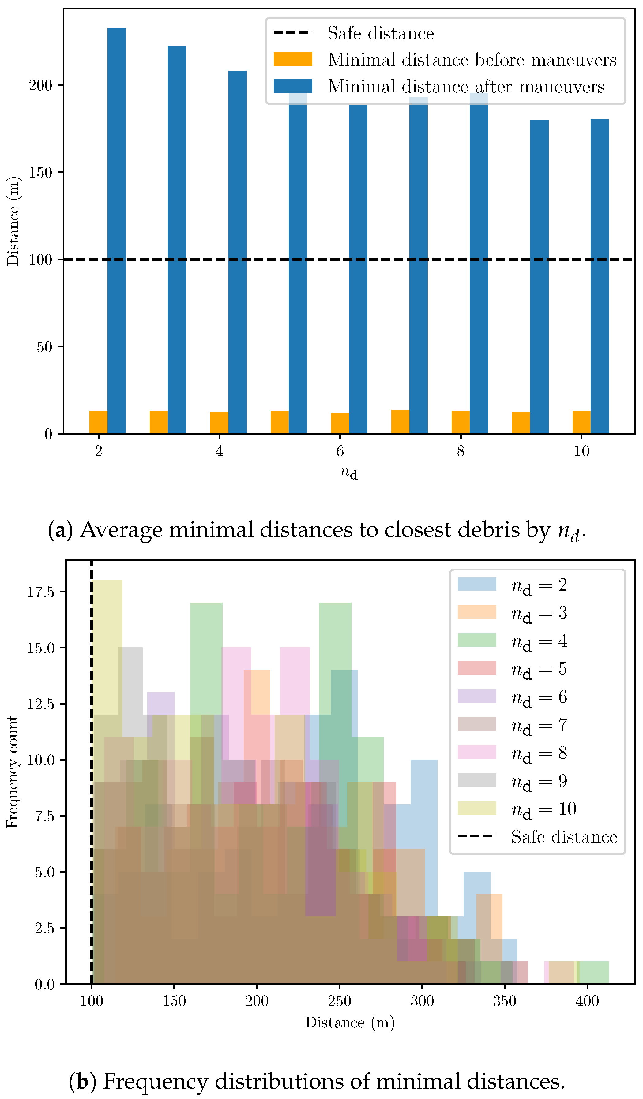
5.2. Simulation Results

A total of 100 test cases were generated for each debris configuration (2–10 pieces) under Scenario 1. In addition, one test case under Scenario 2 is examined. The algorithm demonstrated 100% collision avoidance success rates across all test scenarios.

Result of Scenario 1: In Scenario 1, Figure 6 depicts the minimum distance between the satellite and the debris for different $n_d$. Figure 7 illustrates the maneuver increments required for avoidance. The algorithm operates within a significantly shorter collision time, which also allows it to adopt a smaller safe distance due to high-precision autonomous observation. On the other hand, velocity increment peaks in Figure 7b are observed primarily at the integer multiples of $u_{max}T=0.6$ (e.g., $0.6,1.2$ in the horizontal axis), suggesting that the algorithm terminates maneuvers once the scenario is deemed non-dangerous. These two factors ensure that the fuel consumption remains acceptable even in the short-term avoidance.

Result of Scenario 2: In Scenario 2, the algorithm successfully guided the satellite to separate from the high-speed collision debris, maintaining a minimum distance above 8 km, while simultaneously avoiding three additional low-speed debris pieces, each kept at a minimum distance larger than 100 m. Here, the impulse maneuver listed in Table 7 is used as the initial guess for solving the ELVO-based algorithm, when responding to the unexpected debris threat. Orbital elements for three cases–the unperturbed reference orbit, the avoidance orbit, and the actual orbit after maneuvers–are summarized in

Table 8. Orbital elements comparison for Scenario 2.

Elements	Avoidance Orbit (Impulse)	Reference Orbit (No Maneuver)	Actual Orbit (ELVO-Based)
a (km)	7164.859	7163.280	7165.757
e	2.733 × ${10}^{-3}$	2.524 × ${10}^{-3}$	2.850 × ${10}^{-3}$
i (rad)	1.292	1.292	1.292
$\Omega$ (rad)	0.301	0.301	0.301
$\omega$ (rad)	1.399	1.373	1.414
$\varphi$ (rad)	0.931	0.956	0.914

, following a 600-s simulation. The total velocity change required for all avoidance maneuvers was $1.53$ m/s. The resulting trajectory remained within acceptable tolerances of the avoidance orbit, validating the efficacy of the constrained optimization approach.

Further, Figure 8 presents the algorithm’s average running time. The results show that the average running time for subsequent iterations is significantly shorter than that of the first iteration and the time required for J2 orbit propagation (used for the realistic orbit simulation). The overall performance highlights the algorithm’s potential for on-orbit usage and handling emergent events.

6. Conclusions

This study presents an ELVO-based algorithm that enables satellites to avoid multiple space debris in short-term scenarios, achieving a 100% success rate in avoiding up to 10 debris in the simulations. The algorithm’s error is analyzed under a time-variant linear dynamics model, which is the extension of C-W equations. A compensated safe distance is proposed to ensure the algorithm’s performance. Due to its simple design, it achieves fast online computation speeds, demonstrating its potential for on-orbit autonomous avoidance in future applications. The paper also examines under what circumstances it is appropriate to activate this adaptive algorithm for short-term autonomous avoidance. Recall that our earlier discussion suggests ELVO-RL hybridation as a promising solution for unified short/long-term avoidance, capitalizing on each method’s advantages. Possible integration aspects include the following:

• Develop an RL framework where the ELVO method serves as the reward function, enabling autonomous policy optimization under dynamic orbital constraints.
• Design hybrid imitation learning algorithms that leverage ELVO-generated trajectories as expert demonstrations to improve sample efficiency and safety guarantees.

References

1. Bigdeli, M.; Srivastava, R.; Scaraggi, M. Mechanics of space debris removal: A review. Aerospace 2025, 12, 277. [Google Scholar] [CrossRef]
2. Mehrholz, D.; Leushacke, L.; Flury, W.; Jehn, R.; Klinkrad, H.; Landgraf, M. Detecting, tracking and imaging space debris. ESA Bull. 2002, 109, 128–134. [Google Scholar]
3. Schildknecht, T. Optical surveys for space debris. Astron. Astrophys. Rev. 2007, 14, 41–111. [Google Scholar] [CrossRef]
4. Kessler, D.; Johnson, N. The Kessler syndrome: Implications to future space operations. In Proceedings of the 33rd Annual AAS Guidance and Control Conference, Breckinridge, CO, USA, 5–10 February 2010. [Google Scholar]
5. Muntoni, G.; Montisci, G.; Pisanu, T.; Andronico, P.; Valente, G. Crowded space: A review on radar measurements for space debris monitoring and tracking. Appl. Sci. 2021, 11, 1364. [Google Scholar] [CrossRef]
6. Garcia, L.P.; Furano, G.; Ghiglione, M.; Zancan, V.; Imbembo, E.; Ilioudis, C.; Clemente, C.; Trucco, P. Advancements in on-board processing of synthetic aperture radar (SAR) data: Enhancing efficiency and real-time capabilities. IEEE J. Sel. Top. Appl. Earth Obs. Remote Sens. 2024, 17, 16625–16645. [Google Scholar] [CrossRef]
7. Burroni, T.; Husain, S.; Servidia, P.; Thangavel, K.; Sabatini, R. Constellation of formations for autonomous resident space objects detection using star trackers. In Proceedings of the 74th International Astronautical Congress (IAC), Milan, Italy, 14–18 October 2024. [Google Scholar]
8. Srinithi, B.; Sruthi, N.S.R.; Senthil Kumar, T.; Somasundaram, K.; Ramasamy, M. Enhancing milk yield forecasting in dairy farming using an interpretable machine learning framework. In Proceedings of the 2025 4th International Conference on Sentiment Analysis and Deep Learning (ICSADL), Janakpur, Nepal, 18–20 February 2025; pp. 1549–1557. [Google Scholar]
9. Kim, E.H.; Kim, H.D.; Kim, H.J. A study on the collision avoidance maneuver optimization with multiple space debris. J. Astron. Space Sci. 2012, 29, 11–21. [Google Scholar] [CrossRef]
10. Wang, C.; Chen, D.; Liao, W.; Liang, Z. Autonomous obstacle avoidance strategies in the mission of large space debris removal using potential function. Adv. Space Res. 2023, 72, 2860–2873. [Google Scholar] [CrossRef]
11. Mu, C.; Liu, S.; Lu, M.; Liu, Z.; Cui, L.; Wang, K. Autonomous spacecraft collision avoidance with a variable number of space debris based on safe reinforcement learning. Aerosp. Sci. Technol. 2024, 149, 109–131. [Google Scholar] [CrossRef]
12. Chen, X.; Wang, T.; Qiu, J.; Feng, J. Mission planning on autonomous avoidance for spacecraft confronting orbital debris. IEEE Trans. Aerosp. Electron. Syst. 2025, 61, 4115–4126. [Google Scholar] [CrossRef]
13. Yang, H.; Xie, Z.; Zhao, X.; Jin, M. Ground micro-gravity emulation system for space robot capturing the target satellite. In Proceedings of the 2015 IEEE International Conference on Robotics and Biomimetics (ROBIO), Zhuhai, China, 6–9 December 2015; pp. 2585–2590. [Google Scholar]
14. Artigas, J.; De Stefano, M.; Rackl, W.; Lampariello, R.; Brunner, B.; Bertleff, W.; Burger, R.; Porges, O.; Giordano, A.; Borst, C.; et al. The OOS-SIM: An on-ground simulation facility for on-orbit servicing robotic operations. In Proceedings of the 2015 IEEE International Conference on Robotics and Automation (ICRA), Seattle, WA, USA, 26–30 May 2015; pp. 2854–2860. [Google Scholar]
15. Olivares-Mendez, M.; Makhdoomi, M.R.; Yalçın, B.C.; Bokal, Z.; Muralidharan, V.; Ortiz Del Castillo, M.; Gaudilliere, V.; Pauly, L.; Borgue, O.; Alandihallaj, M.; et al. Zero-G Lab: A multi-purpose facility for emulating space operations. J. Space Saf. Eng. 2023, 10, 509–521. [Google Scholar] [CrossRef]
16. Schlotterer, M.; Edlerman, E.; Fumenti, F.; Gurfil, P.; Theil, S.; Zhang, H. On-ground testing of autonomous guidance for multiple satellites in a cluster. In Proceedings of the 8th International Workshop on Satellite Constellations and Formation Flying, Delft, The Netherlands, 8–10 June 2015; p. 386043. [Google Scholar]
17. Fiorini, P.; Shiller, Z. Motion planning in dynamic environments using velocity obstacles. Int. J. Robot. Res. 1998, 17, 760–772. [Google Scholar] [CrossRef]
18. Vesentini, F.; Muradore, R.; Fiorini, P. A survey on Velocity Obstacle paradigm. Robot. Auton. Syst. 2024, 174, 104645. [Google Scholar] [CrossRef]
19. Van Den Berg, J.; Lin, M.; Manocha, D. Reciprocal velocity obstacles for real-time multi-agent navigation. In Proceedings of the 2008 IEEE International Conference on Robotics and Automation, Pasadena, CA, USA, 19–23 May 2008; pp. 1928–1935. [Google Scholar]
20. Van Den Berg, J.; Guy, S.J.; Lin, M.; Manocha, D. Reciprocal n-body collision avoidance. In Proceedings of the Robotics Research: The 14th International Symposium ISRR; Springer: Berlin/Heidelberg, Germany, 2011; pp. 3–19. [Google Scholar]
21. An, R.; Guo, S.; Zheng, L.; Hirata, H.; Gu, S. Uncertain moving obstacles avoiding method in 3D arbitrary path planning for a spherical underwater robot. Robot. Auton. Syst. 2022, 151, 104011. [Google Scholar] [CrossRef]
22. Li, A.; Guo, S.; Li, C.; Yin, H.; Liu, M.; Shi, L. A moving obstacle avoidance strategy-based collaborative formation for the bionic multi-underwater spherical robot control system. Ocean. Eng. 2025, 329, 121120. [Google Scholar] [CrossRef]
23. Shiller, Z.; Large, F.; Sekhavat, S. Motion planning in dynamic environments: Obstacles moving along arbitrary trajectories. In Proceedings of the 2001 IEEE International Conference on Robotics and Automation, Seoul, Republic of Korea, 21–26 May 2001; Volume 4, pp. 3716–3721. [Google Scholar]
24. Jenie, Y.I.; van Kampen, E.J.; de Visser, C.C.; Ellerbroek, J.; Hoekstra, J.M. Three-dimensional velocity obstacle method for uncoordinated avoidance maneuvers of unmanned aerial vehicles. J. Guid. Control. Dyn. 2016, 39, 2312–2323. [Google Scholar] [CrossRef]
25. Lin, Z.; Castano, L.; Mortimer, E.; Xu, H. Fast 3D collision avoidance algorithm for fixed wing UAS. J. Intell. Robot. Syst. 2020, 97, 577–604. [Google Scholar] [CrossRef]
26. Sullivan, J.; Grimberg, S.; D’Amico, S. Comprehensive survey and assessment of spacecraft relative motion dynamics models. J. Guid. Control. Dyn. 2017, 40, 1837–1859. [Google Scholar] [CrossRef]
27. De Maesschalck, R.; Jouan-Rimbaud, D.; Massart, D.L. The mahalanobis distance. Chemom. Intell. Lab. Syst. 2000, 50, 1–18. [Google Scholar] [CrossRef]
28. Leleux, D.; Spencer, R.; Zimmerman, P.; Propst, C.; Frisbee, J.; Wortham, M.; Heilman, W. Probability-based space shuttle collision avoidance. In Proceedings of the SpaceOps 2002 Conference, Houston, TX, USA, 9–12 October 2002; p. 50. [Google Scholar]
29. Broucke, R.A. Solution of the elliptic rendezvous problem with the time as independent variable. J. Guid. Control. Dyn. 2003, 26, 615–621. [Google Scholar] [CrossRef]
30. Gonzalo, J.L.; Colombo, C.; Di Lizia, P. Analytical framework for space debris collision avoidance maneuver design. J. Guid. Control. Dyn. 2021, 44, 469–487. [Google Scholar] [CrossRef]
31. Li, J.S.; Yang, Z.; Luo, Y.Z. A review of space-object collision probability computation methods. Astrodynamics 2022, 6, 95–120. [Google Scholar] [CrossRef]
32. Patera, R.P. General method for calculating satellite collision probability. J. Guid. Control. Dyn. 2001, 24, 716–722. [Google Scholar] [CrossRef]
Figure 1. Illustration of Velocity Obstacle, projected into 2D space.
Aerospace 12 00402 g001
Figure 2. Illustration of Equivalent Linear Velocity Obstacle. The debris moves with a varying velocity v i ( t ) . At time t 1 , the debris reaches position r i ( t 1 ) with velocity v i ( t 1 ) , as indicated by the dashed circle r i ( t 1 ) . The dashed circle r ^ i ( t 0 ) represents a virtual object that will reach r i ( t 1 ) at time t 1 with a constant velocity of v i ( t 1 ) . The ELVO of the satellite with respect to the i-th debris at time t 1 is defined by the VO of the satellite with respect to this virtual object.
Aerospace 12 00402 g002
Figure 3. Values of Δ Φ r r and Δ Φ r v with respect to δ t C .
Aerospace 12 00402 g003
Figure 4. Values of Φ r v ( t , s + t 0 ) Φ r v ( t , t 0 ) and Δ Φ r v ( t C , t 0 ) .
Aerospace 12 00402 g004
Figure 5. Space debris collision avoidance procedure.
Aerospace 12 00402 g005
Figure 6. Minimal distances between satellite and closest debris after maneuvers for Scenario 1.
Aerospace 12 00402 g006
Figure 7. Maneuver increments for Scenario 1. (a) Average maneuver increments by n d ; (b) Frequency distributions of maneuver increments.
Aerospace 12 00402 g007aAerospace 12 00402 g007b
Figure 8. Average running time of the algorithm shown in logarithmic scale. Both the propagation of the orbit and the solving of the ELVO problem are invoked once per programming iteration, i.e., for each T = 20 s .
Aerospace 12 00402 g008