An Actor–Critic-Based Hyper-Heuristic Autonomous Task Planning Algorithm for Supporting Spacecraft Adaptive Space Scientific Exploration

Abstract

Traditional spacecraft task planning has relied on ground control centers issuing commands through ground-to-space communication systems; however, as the number of deep space exploration missions grows, the problem of ground-to-space communication delays has become significant, affecting the effectiveness of real-time command and control and increasing the risk of missed opportunities for scientific discovery. Adaptive Space Scientific Exploration requires that spacecraft have the ability to make autonomous decisions to complete known and unknown scientific exploration missions without ground control. Based on this requirement, this paper proposes an actor–critic-based hyper-heuristic autonomous mission planning algorithm, which is used for mission planning and execution at different levels to support spacecraft Adaptive Space Scientific Exploration in deep space environments. At the bottom level of the hyper-heuristic algorithm, this paper uses the particle swarm optimization algorithm, grey wolf optimization algorithm, differential evolution algorithm, and positive cosine optimization algorithm as the basic operators. At the high level, a reinforcement learning strategy based on the actor–critic model is used, combined with the network architecture, to construct a framework for the selection of advanced heuristic algorithms. The related experimental results show that the algorithm can meet the requirements of Adaptive Space Scientific Exploration, and exhibits a quality solution with higher comprehensive evaluation in the test. This study also designs an example application of the algorithm to a space engineering mission based on a collaborative sky and earth control system to demonstrate the usability of the algorithm. This study provides an autonomous mission planning method for spacecraft in the complex and ever-changing deep space environment, which supports the further construction of spacecraft autonomous capabilities and is of great significance for improving the exploration efficiency of deep space exploration missions.

1. Introduction

Traditional spacecraft payload operation modes predominantly rely on ground control centers to issue commands through Earth–space communication systems, guiding spacecraft in task planning, orbital adjustments, data collection, and processing. This approach is highly efficient in Earth–Moon systems or near-Earth orbital missions, where communication delays are minimal, allowing ground control centers to monitor spacecraft status almost in real time and adjust mission plans accordingly. However, as space exploration progressively delves into the unknown realms of deep space, accompanied by an increasing number of deep space exploration projects, this mode of operation faces significant challenges. The extended distances of Earth–space communication result in considerable communication delays, adversely affecting real-time command control and increasing the risk of missing scientific discovery opportunities. Moreover, the uncertainty of deep space exploration environments, coupled with the often unknown nature of exploration targets, demands a higher level of spacecraft autonomy.

Adaptive Space Scientific Exploration (ASSE) refers to the capability of spacecraft to make autonomous decisions based on their limited capabilities, resources, and knowledge, without reliance on ground control centers, to fulfill both known and unknown scientific exploration tasks. This requires spacecraft to determine the necessary tasks and objectives based on telemetry data, health status, operational parameters, and the real-time conditions of deep space, ensuring high operational precision, robust performance, strong adaptability to the environment, and longevity. Implementing ASSE necessitates the development of a system architecture platform that supports intelligent capabilities for spacecraft, along with leveraging a variety of intelligent technologies to enhance autonomy.

Viewed through the lens of the integrated electronic systems’ capabilities within spacecraft, the ASSE paradigm mandates the provision of several pivotal capabilities for spacecraft. These include the ability to discover and identify both unseen and known scientific targets, an autonomous mission planning capability for executing requisite tasks or instructions, an autonomous task execution management capability, and a comprehensive system of self-management and monitoring capability. Notably, the spacecraft’s autonomous mission planning capability—rooted in the outcomes of target identification and significantly impacting the operational state of the spacecraft subsequent to identification—emerges as a seminal research topic within the ambit of spacecraft’s autonomous operation and control. Deploying such planning methodologies directly on spacecraft, as opposed to terrestrial control systems, necessitates heightened demands on the systems’ and algorithms’ flexibility, robustness, and reliability.

Within the domain of autonomous operation and control of spacecraft, Daniel D. Dvorak and his colleagues have pioneered a revolutionary operational paradigm termed goal-driven operation [1]. This paradigm marks a fundamental shift in operational underpinnings from executing a sequenced set of commands to a declarative specification of operational intents, thereby facilitating guidance via well-defined objectives. This method significantly augments operational robustness amidst uncertainties and amplifies the system’s autonomous decision-making capabilities through the lucid articulation of operational intents.

In this study, the essence of spacecraft task planning is fundamentally oriented toward the planning of “objectives”. During autonomous operation, spacecraft are required to complete numerous pending tasks, among which there are variations in priority, resource consumption, and scientific detection needs. The sequence in which tasks are executed significantly impacts the spacecraft’s operational status, which in turn directly affects the efficiency, quality, and stability of scientific detection. Therefore, the development of a planning algorithm that is both adaptable to the deep space environment and capable of effectively addressing these challenges is particularly crucial.

Confronted with the dynamic nature and unpredictability of space exploration, the limitations of existing planning methods are increasingly evident. These traditional approaches are largely based on the predictability of a pre-set environment, utilizing pre-programmed instructions and models. Researchers choose appropriate heuristic methods to optimize task sequences based on controlled environments. However, the effectiveness of these methods relies on accurate environmental predictions, making them ill-suited for unknown or changing objectives. The complexity of deep space exploration demands that planning algorithms possess a high degree of flexibility and adaptability to address unforeseen challenges. In short, a singular algorithm cannot guarantee superiority across all environments and instances in deep space due to a lack of necessary adaptive mechanisms. This discrepancy can lead to difficulties in estimating convergence speed and optimization efficiency, as well as adapting to the unknown environments of deep space, missing opportunities for scientific discovery, and sometimes even jeopardizing the success of missions. This situation underscores the urgent need to move beyond traditional methods and adopt more advanced planning strategies.

Hyper-heuristic algorithms offer a novel approach to tackling such issues by operating at a higher level of abstraction. This method manages and manipulates a series of low-level heuristics (LLH) to forge new heuristic solutions, applicable to a wide array of combinatorial optimization problems [2]. The process encompasses two principal layers: initially, at the problem’s lower level, algorithms build mathematical models grounded in the problem’s representation and characteristics, designing specific solutions within a predetermined meta-heuristic framework. At a higher heuristic layer, an “intelligent computation expert” role is established, employing an efficient management and manipulation mechanism to derive new heuristic solutions from the lower level’s algorithm library and characteristic information [3]. This design enables the intelligent computation expert to autonomously select the most fitting heuristic algorithm based on current environmental data, allowing, in theory, for adaptability to various environmental conditions if the lower-level algorithms are judiciously chosen.

Traditional hyper-heuristic algorithm research has primarily focused on methods based on Simple Random [4], Choice Function [5], Modified Choice Function [6], Tabu Search [7], Ant Colony [8], and reinforcement learning [9,10,11]. Recently, integrating hyper-heuristic algorithms based on reinforcement learning with neural network technologies has emerged as a growing research area. This new direction aims to develop more accurate and reliable “intelligent computation experts” through deep reinforcement learning methods [12], capitalizing on neural networks’ non-linearity, adaptability, robustness, and parallel information processing capabilities. Deep reinforcement learning utilizes the perceptual power of deep learning to comprehend the environment, combined with the decision-making mechanisms of reinforcement learning, to identify optimal behavioral strategies across various settings [13]. By amalgamating deep reinforcement learning methods, optimized neural network architectures, and diverse heuristic algorithms, this approach not only merges the strengths of multiple technologies but also crafts algorithms specifically for deep-space mission planning, thereby enhancing spacecraft’s planning capabilities in the face of complex and changing environments.

Based on this, the main contributions of this paper are as follows:

• Relying on the philosophy of building autonomous capabilities onboard spacecraft and the “goal-driven” methodology, this study introduces a spacecraft task planning framework designed to meet the requirements of adaptive scientific exploration and conducts mathematical modeling of the planning issue.
• Based on a mathematical model, we designed an Actor–Critic-based Hyper-heuristic Autonomous Task Planning Algorithm (AC-HATP) to support spacecraft Adaptive Space Scientific Exploration.
• At the lower tier of hyper-heuristic algorithms, by considering three aspects, namely global search capabilities, quality of solution optimization, and speed of convergence, we selected and designed suitable heuristic algorithms, establishing an algorithmic library.
• At the higher tier of hyper-heuristic algorithms, we employed a reinforcement learning strategy based on the actor–critic model, in conjunction with the network architecture, to construct an advanced heuristic algorithm selection framework.
• Through designed experiments, our research validated that the algorithm meets the needs of adaptive scientific exploration. Compared with other algorithm types, it was demonstrated that our approach achieves faster convergence speeds and superior solution quality in addressing deep space exploration challenges.

2. Related Work

The problem of autonomous mission planning for spacecraft can be defined as an optimization issue of how to efficiently allocate a series of tasks to satellites within the constraints of limited satellite maneuverability and fixed time windows, aiming to maximize payload utilization efficiency and optimize target information collection [14]. This represents a variant of common planning optimization problems. Planning typically involves specifying a problem’s initial and target states, along with a description of actions, requiring the automatic discovery of a sequence of actions that allows the system to transition from the initial state to the target state [15]. In this paper, we categorize autonomous spacecraft mission planning methods into three main groups for discussion: traditional methods (including planning based on predicate logic, network graphs, and timelines), heuristic algorithm methods, and reinforcement learning methods.

2.1. Traditional Methods of Autonomous Task Planning

The earliest methods for addressing planning problems relied on strict linguistic and logical structures for problem description and resolution. At this stage, various planning representation methods existed, such as first-order logic [16] and situation calculus [17], which served as second-order logic languages depicting the dynamics of the world. Subsequently, researchers like Nillson introduced the STRIPS planning description methodology, marking the preliminary formation of methodologies within the planning domain [18]. Building upon the foundation of STRIPS, the planning research domain gradually developed a mature description language known as PDDL. Then, Mc Dermott [19] formally proposed the Planning Domain Definition Language (PDDL), which has since undergone continuous refinement and development, resulting in multiple versions including PDDL 2.1 [20], PDDL 2.2 [21], and PDDL 3.0 [22], and even the advent of the PDDL+ version [23]. Owing to its outstanding features, PDDL has been widely applied in spacecraft mission planning, particularly in autonomous mission planning on satellites, for task description and modeling. For instance, researchers like ZHU Liying, in the domain of autonomous flight intelligent planning for small body exploration, through designing knowledge models based on PDDL, mathematical models based on CSP, and solving algorithms based on genetic strategies, effectively achieved efficient task management and simplified operational processes [24]. Researchers like Emma, by integrating task planning with execution monitoring, have enhanced the autonomous operational capabilities of space robots, especially through enhancing the robots’ intelligent task processing with PDDL [25]. Li Xuan [26] used PDDL to model and validate inter-satellite transmission mission planning in a collaborative satellite network where microwave and laser links coexist. Researchers such as Ma Manhao have utilized PDDL to focus on the constraints between observation tasks, modeling from the aspects of constraints, activities, and planning objectives, thus constructing an applied mission planning model for Earth Observation Satellites (EOSs) [27]. Researchers like Chen [28], based on a deep analysis of the characteristics of imaging satellite mission planning issues, used PDDL to address duration constraints, complex resource constraints, and special external resource constraints, establishing a mission planning model for urban and rural satellites. Xue [29] established an autonomous mission planning model for satellites in emergency situations, achieved the definition of constraints based on PDDL, and constructed a model that comprehensively considers the constraints of satellite platforms and payloads.

In the practical planning process, especially when facing time-sensitive planning issues, relying solely on the descriptive method of predicate propositional logic can be challenging to adequately describe factors such as time constraints. Conversely, the timeline model, with its straightforward and intuitive feature of time constraints, becomes an ideal choice for satellite mission planning with lower concurrent demands and more singular tasks. For example, researchers like Xu [30], in the study of autonomous mission planning for deep space probes, have adopted representation methods based on states and state timelines to describe the tasks of the probes and their constraint relationships. Researchers like Wang [31], through an object-oriented formal description method, categorized domain knowledge, including four models such as the timeline model, and simplified the method of establishing constraints. NASA’s ASPEN system [32], with its iterative repair philosophy, has developed a variety of reasoning mechanisms and developed a new type of mission planning method centered on the state timeline. The European Space Agency, based on the ASPI system, models the timeline pattern of scientific tasks, considering defects as the core object, and drives the planning process through collecting, selecting, and solving defects [33].

Additionally, various methodologies have been adopted for solving spacecraft mission planning challenges. The SPLKE system in the United States, designed to cater to the servicing needs of the Hubble Space Telescope, employs an algorithm based on the Constraint Satisfaction Problem (CSP) for task planning [34]. Jiang [35] have devised a task planning strategy based on constraint grouping. This method, which places a premium on action constraints, circumvents the issue of diminished constraint capacity with the expansion of problem size. Du [36] has utilized colored Petri nets for system modeling, categorizing the model into a top-level model, control model, target imaging mission planning model, and image transmission mission planning model, thereby applying this planning approach to imaging satellites. Liang [37] have designed an autonomous mission planning method based on a priority approach. This method, which leverages timeline technology and takes into consideration task priorities, facilitates the effective planning of task sequences. Bucchioni [38] proposed an innovative rendezvous strategy in cis-lunar space, combining passive and active collision avoidance to ensure safety during the approach to the Moon’s L2 point, filling a gap in the literature on autonomous guidance systems in the presence of third-body influences and significantly advancing the field of autonomous mission planning.

2.2. Task Planning Based on Heuristic and Metaheuristic Algorithms

Heuristic algorithms are strategies that rely on experience and intuition to find solutions, particularly suitable for scenarios where precise solutions cannot be obtained within a reasonable time frame. Although heuristic algorithms do not guarantee the optimal solution, they often provide a satisfactory solution within an acceptable timeframe. For example, NASA’s DS-1 spacecraft utilized a planning-space-based heuristic algorithm for mission planning. This method demonstrates excellent scalability and partial orderliness in outcomes, thereby enhancing the flexibility of execution planning [39]. Xue [29] employed Relaxation-based Graph Planning (RGP), an Enhanced Hill-Climbing Method, and Greedy Best-First Search (GBFS) to segment the satellite mission planning into sequence planning and time scheduling. Chang et al. [40] addressed the challenges in planning for optical video satellites with variable imaging durations, proposing a Simple Heuristic Greedy Algorithm (SHGA) to enhance its performance. Zhao et al. [41] explored the scheduling issues of satellite observation missions, implementing a task clustering planning algorithm to improve the observational efficiency of agile satellites, using Tabu algorithms to generate local and global observation paths within the clustered regions. Jin et al. [42] introduced a heuristic estimation strategy and search algorithm to enhance planning efficiency on spacecraft, with experimental results showing superior performance compared to Europa2. The optimal design of an active space junk removal mission similar to the time-dependent orientation problem was solved with the A* algorithm by Federici [43].

Meta Heuristic Algorithms (MHAs) represent a sophisticated optimization strategy, aimed at guiding and controlling heuristic search processes to identify the most optimal solutions possible within a solution space. The primary advantage of these algorithms is their independence from specific domain knowledge, which endows them with significant versatility, allowing their application across a wide range of optimization challenges. Common metaheuristic algorithms include genetic algorithms, simulated annealing, and particle swarm optimization. Notably, these algorithms have been extensively explored for the autonomous task planning of spacecraft. For instance, Long [44] developed an autonomous management and collaboration architecture for multi-agent systems tailored to the complexity and variability of managing multi-satellite systems. They introduced a hybrid genetic algorithm with simulated annealing (H-GASA) to address autonomous mission planning challenges in multi-satellite cooperation. Xiao et al. [45] investigated a hybrid optimization algorithm that integrates tabu search and an enhanced ant colony optimization algorithm, designed to tackle the maintenance task planning of large-scale space solar power stations. Wang [46] considered time and resource constraints, proposed the concept of dynamic resources and devised an individual coding rule based on fixed-length integer sequence coding to reduce the search space. They introduced a genetic algorithm that combines multi-mode crossover mutation, and designed a replanning algorithm framework based on rolling horizon replanning. Zhao and Chen [47], in the context of Earth observation satellite design, incorporated two generations of competitive technologies and an optimal retention strategy to address local multi-conflict observation tasks with an improved genetic algorithm. Feng et al. [48] designed a payload mission planning algorithm based on genetic algorithms capable of generating a complete command sequence according to tasks and directives, thereby implementing an autonomous operation system architecture for spacecraft based on multi-agent systems.

2.3. Task Planning Based on Reinforcement Learning

Reinforcement learning (RL) is an algorithm that learns optimal behavioral strategies through a system of rewards and punishments. In the context of spacecraft task planning, RL algorithms refine actions through a process of defining functions and actions, utilizing feedback on the effects of these actions on the final outcome to achieve an optimal solution. Despite the inherent conflict between the exploratory nature of RL and the high reliability requirements of spacecraft, which has limited its application in the aerospace field, ongoing research in this area has led to the exploration of this artificial intelligence technique in spacecraft task planning and decision-making processes. Harris et al. [49] have applied deep reinforcement learning (DRL) to spacecraft decision-making challenges, addressing issues of problem modeling, dimensionality reduction, simplification using expert knowledge, sensitivity to hyperparameters, and robustness, and ensured safety by integrating appropriately designed control techniques. Hu et al. [9] proposed an end-to-end DRL-based step planner named SP-ResNet for global path planning of planetary rovers, employing a dual-branch residual network for action value estimation, validated on the real lunar terrain of the CE2TMap2015 dataset. Huang et al. [50] explored the scheduling of Earth observation satellite missions, adopting a deep deterministic policy gradient algorithm to address the problem of continuous-time satellite mission scheduling, with experimental results indicating superiority over traditional meta-heuristic optimization algorithms. Wei et al. [51] introduced a method based on deep reinforcement learning and parameter transfer (RLPT) for iteratively solving the Multi-Objective Agile Earth Observing Satellite Scheduling Problem (MO-AEOSSP), surpassing three classical multi-objective evolutionary algorithms (MOEAs) in terms of solution quality, distribution, and computational efficiency, demonstrating high universality and scalability. Zhao et al. [52] proposed a dual-phase neural combinatorial optimization method based on reinforcement learning for the scheduling of agile Earth observing satellites (AEOSs). Eddy and Kochenderfer [53] presented a semi-Markov decision process (SMDP) formulation for satellite mission scheduling that considers multiple operational goals and plans transitions between different functional modes. This method performed comparably to baseline methods in single-objective scenarios with faster speed and achieved higher scheduling rewards in multi-objective scenarios.

2.4. Summary of Related Work

The research for the related work can be summarized as shown in

Table 1. Summary of research in autonomous mission planning methods.

Category	Methods	Features	Applications	Limitations
Traditional Methods	- First-order Logic - STRIPS - Situation Calculus - PDDL Variants	Logical rigor and strict syntactic structures Supports complex problem descriptions Allows detailed domain modeling	- Deep Space 1 (DS1) - Cassini–Huygens mission - Mars Rover missions	Inflexible in dynamic, unpredictable environments typical of deep space Too rigid for complex scenarios
Heuristic Algorithms	- RGP - GBFS - SHGA	Employs intuitive solution paths Facilitates quick convergence to satisfactory solutions Scalable to large problem sizes	- Hubble Space Telescope Servicing Missions - Earth Observing-1 (EO-1) - Autonomous Nano Satellite Guardian Evaluating Local Space (ANGELS)	Suboptimal in complex, multi-variable environments Often fails to find the global optimum, limited by specific heuristic rules
Meta-Heuristic Algorithms	- GA - SA - PSO - H-GASA	Capable of exploring large search spaces Adaptable to varying problem constraints Can find near-optimal solutions with sufficient computational resources	- Swarm satellite systems - DARPA’s Orbital Express - Galaxy 15 satellite reactivation	It may require extensive computation Can struggle with convergence in highly complex environments Generalizations across different tasks can be poor
Reinforcement Learning	- DRL - DQN - DDPG - RLPT - SMDP	Continuous learning from environment interaction Adjusts strategies based on reward feedback Suitable for dynamic adaptation	- Lunar Gateway (NASA’s planned space station in lunar orbit) - SPHERES satellites on the ISS - Mars Sample Return Rover	Limited by the need for large amounts of training data Impractical for online training in deep space Can be overly sensitive to hyperparameters and initial conditions

.

In the complex and uncertain environment of deep space, traditional rule-based methods are limited in flexibility, making it challenging to meet the requirements for problem resolution. Heuristic and meta-heuristic algorithms, constrained by their generalization capabilities and environmental adaptability, require integration with a high-level architecture of hyper-heuristic algorithms, and the construction of a heuristic algorithm library at the lower level to cover as diverse a range of potential environmental states as possible. Regarding reinforcement learning methods, given the unique environmental constraints in deep space, using online reinforcement learning to train models is impractical. For offline reinforcement learning methods, the significant increase in environmental uncertainty may result in trained models that fail to meet practical needs, presenting challenges similar to those faced by meta-heuristic algorithms. Therefore, considering the autonomous learning capabilities of reinforcement learning, although it cannot be directly applied to spacecraft onboard task planning in deep space, it can serve as an upper-layer “expert system” within a hyper-heuristic algorithm framework, responsible for selecting appropriate algorithms. By designing a sufficiently rich algorithm library, and utilizing reinforcement learning for algorithm selection, the system can adapt to a broad and variable environment, thus enhancing the model’s adaptability. Moreover, the limited action space of this type of reinforcement learning significantly reduces the difficulty of training the model.

Consequently, this study proposes a hyper-heuristic algorithm framework with reinforcement learning at the upper layer and meta-heuristic algorithms at the base layer, aimed at enhancing the adaptability of spacecraft in the uncertain conditions of deep space.

3. Framework and Modeling for Spacecraft Onboard Autonomous Task Planning

According to the literature [54], spacecraft operating in deep space can have their intelligence levels classified into three categories: “automatic”, “autonomous”, and “self-governing”. In this classification, “automatic” spacecraft are capable of substituting manual operations with software, hardware, and algorithms, though their operations still depend on human intervention, such as receiving and executing commands. At the “autonomous” level, spacecraft simulate human operational processes and are able to independently carry out simple task executions and self-learning, such as executing commands in a pre-determined sequence. “Self-governing” spacecraft are capable of analyzing their current state and surrounding environment, and making rational decisions based on this analysis to more effectively achieve predefined objectives.

ASSE poses a challenge for spacecraft intelligence capabilities to transition from autonomous to self-governing operation, ensuring stable and continuous functioning in the complex environment of deep space. This requires comprehensive coordination and integration across three critical aspects: spacecraft architectural design, data description methods, and algorithm development. Firstly, it is essential to design a spacecraft architecture that supports self-governing capabilities, facilitates the operation and deployment of relevant algorithms, and controls the spacecraft based on the outcomes of these algorithms. Secondly, to enable effective data interchange between the architecture and algorithms, a suitable data description format must be designed. Finally, problem-specific algorithms need to be developed and deployed on the architecture using established data description formats.

3.1. Target-Driven and Task-Level Objective Commands

Traditional spacecraft operations primarily involve the method of data injection to transmit action commands to the spacecraft. This method is widely used due to its directness and reliability. However, with the increasing uncertainties of deep space exploration missions and extended communication delays, this approach can result in missed opportunities for scientific objectives, thus impacting the efficiency of the exploration. As the number of spacecraft increases and operational modes become more mature, some routine operations can transition from manual to automatic execution. Consequently, the scope of spacecraft operations should shift from specific “actions” to specific “objectives”, allowing the spacecraft to autonomously select and execute commands that align with the current objectives. This operational mode is referred to as “goal-driven”.

According to research by MAULLO [55], the concept of “goal-driven” operations involves shifting the basis of operations from a sequence of command instructions to declarative operational intentions, or goals, thereby reducing the workload of operators and allowing them to focus on “what” to do rather than “how” to do it. This method enhances the system’s autonomy and its ability to respond to unpredictable environments. By clearly defining operational intentions, the system can verify the successful achievement of objectives and, when necessary, employ alternative methods to achieve these goals [1].

Through the use of “goal-oriented” commands, spacecraft can encapsulate specific sequences of behavioral instructions, thereby concentrating on the objectives to be fulfilled rather than the operational details of the commands themselves. These commands do not have a fixed design framework; each organization and spacecraft manufacturer can customize the command format based on their specific requirements. In this study, given the emphasis on planning for spacecraft mission objectives, these are designated as “Task-Oriented Commands” (TOCs) [56].

This research utilizes TOCs as the fundamental unit of mission planning. When a spacecraft is required to manage multiple TOCs simultaneously, it must holistically assess the current resource information, the resource consumption associated with the objectives, and the environmental conditions in which the spacecraft operates. An optimal mission execution strategy is then selected, aiming to achieve maximum efficiency and minimal resource consumption in the shortest possible time and with the fewest iterations.

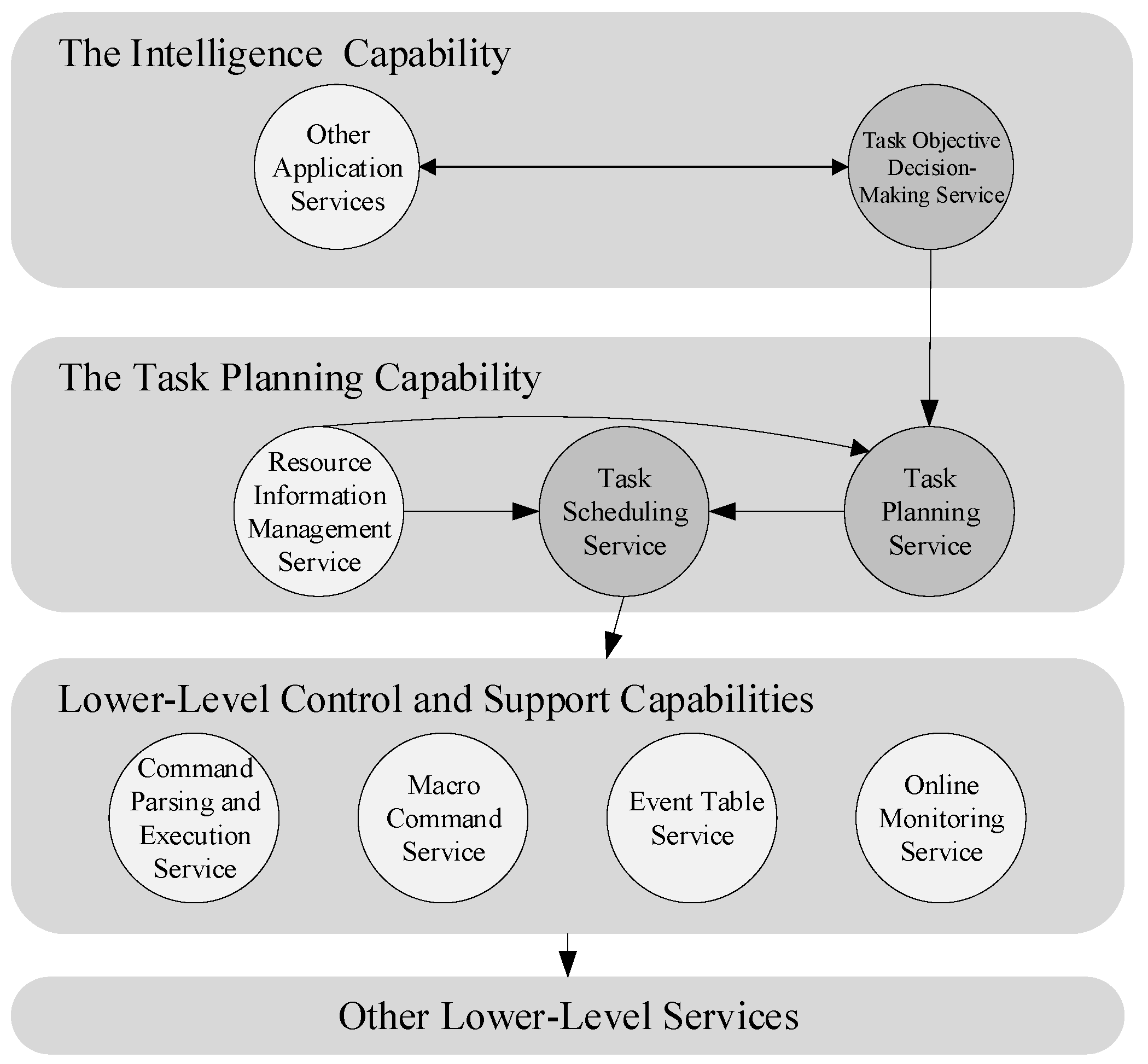
3.2. Spacecraft Autonomous and Task Planning Framework

The task planning framework in this study is based on the intelligent flight software architecture for spacecraft proposed by Lyu [57]. This architecture incorporates the Spacecraft Onboard Interface Services (SOIS), selecting service according to the needs of intelligent capabilities. The entire framework is segmented into the subnet layer, application support layer, and application layer, with the task planning module positioned at the upper echelon of the application layer. This study focuses on the design of task planning capabilities at the higher level of the application layer of the framework.

The autonomous task planning capabilities of the spacecraft comprise three main services: decision-making, planning, and scheduling. The relationship between these services and the overall architecture is depicted in Figure 1. The decision-making service involves the spacecraft generating and formulating task objectives based on the current environment and status, outputting several TOCs. The planning service is responsible for determining the execution sequence of various TOCs and generating a TOC execution sequence. The scheduling service entails decomposing each TOC into specific actions and commands executable by the spacecraft, ensuring that each TOC’s implementation effectively reaches the intended target state. Detailed descriptions of these services and their inputs and outputs are provided in

Table 2. Summary of autonomous spacecraft task planning processes.

Name	Decision-Making	Planning	Scheduling
Input	Spacecraft’s current environment and status	Unordered set of task-level objective commands without timestamps	Task-level objective commands
Output	Task-level objective commands and their parameters	Timestamped sequence of task-level objective commands	Schedule-level commands Primitive-level commands
Problem Category	Decision problem	Optimization problem	Decomposition problem

. In summary, the task planning capabilities generate appropriate TOCs based on the spacecraft’s environment and status and plan their execution sequence. Subsequently, during implementation, these TOCs are broken down into concrete, executable commands, enabling the spacecraft to autonomously generate action commands in response to the current environment, thus fulfilling the requirements of ASSE.

This study aims to design a task planning service that optimizes the execution sequence of TOCs based on the onboard environment of the spacecraft, thereby enhancing the efficiency of task execution and the computational speed of the algorithm.

3.3. Mathematical Description of Spacecraft Autonomous Mission Planning Problem

This study explores the sequence planning problem for TOCs, with the objective of maximize scientific exploration benefits within the shortest possible operational duration, thereby optimizing the cost–benefit ratio. The spacecraft is required to methodically execute each mission objective until all known targets are completed. This issue represents a variant of the traveling salesman problem (TSP), a combinatorial optimization challenge that seeks to determine the shortest route by which a salesman departs from a city, visits each other city exactly once, and returns to the starting city, ensuring that the total path length (or cost) is minimized [58]. In this research, the total cost is defined in terms of the cost–benefit ratio, with additional considerations given to resources and environmental factors during the completion of each task.

Table 3. Summary of symbols and definitions for the task sequence planning model.

Term	Definition
$T$	$\mathrm{Represents} \mathrm{the} \mathrm{set} \mathrm{of} \mathrm{TOCs}, T=\left\{t_1,t_2,\dots ,t_n\right\}$
$x_{ijk}$	$\mathrm{Equals} 1 \mathrm{if} \mathrm{task} j$$\mathrm{is} \mathrm{executed} \mathrm{at} \mathrm{position} k$$\mathrm{following} \mathrm{task} i$, otherwise 0
$d_{ij}^m$	$\mathrm{The} \mathrm{cost} \mathrm{in} \mathrm{the} m$-th dimension (e.g., time, fuel consumption) of transitioning from task i to task j
$r_i^n$	$\mathrm{The} \mathrm{amount} \mathrm{of} \mathrm{the} n$$-\mathrm{th} \mathrm{type} \mathrm{of} \mathrm{resource} \mathrm{required} \mathrm{to} \mathrm{perform} \mathrm{task} i$
$R_{\mathrm{total}}^n$	$\mathrm{Total} \mathrm{quantity} \mathrm{of} \mathrm{the} n$-th type of resource
$e_{ij}^n$	$\mathrm{The} \mathrm{amount} \mathrm{of} \mathrm{the} n$$-\mathrm{th} \mathrm{type} \mathrm{of} \mathrm{resource} \mathrm{obtained} \mathrm{after} \mathrm{completing} \mathrm{task} j$$\mathrm{through} \mathrm{task} i$
$c_{ij}$	$\mathrm{Cost}–\mathrm{benefit} \mathrm{ratio} \mathrm{from} \mathrm{task} i$$\mathrm{to} \mathrm{task} j$
$P_{\mathrm{m}\mathrm{i}\mathrm{n}}$	Minimum cost–benefit ratio threshold
$W_{ij}^n$	$\mathrm{Time} \mathrm{window} \mathrm{available} \mathrm{for} \mathrm{resource} n$$\mathrm{between} \mathrm{tasks} i$$\mathrm{and} j$; equals 1 if within the window, otherwise 0
${\tau }_{\max }^{ij}$	$\mathrm{Maximum} \mathrm{allowable} \mathrm{time} \mathrm{interval} \mathrm{between} \mathrm{tasks} i$$\mathrm{and} j$
$M$	$\mathrm{A} \mathrm{sufficiently} \mathrm{large} \mathrm{number} \mathrm{ensuring} \mathrm{that} \mathrm{certain} \mathrm{constraints} \mathrm{are} \mathrm{inactive} \mathrm{when} x_{ijk}=0$
$v_i^n$	$\mathrm{The} \mathrm{consumption} \mathrm{rate} \mathrm{of} \mathrm{the} n$$-\mathrm{th} \mathrm{type} \mathrm{of} \mathrm{resource} \mathrm{during} \mathrm{the} \mathrm{execution} \mathrm{of} \mathrm{task} i$
$u_i$	The relative position of task i during task execution.
$t_{ij}$	The time required to transition from task i to task j
$V_{ij}$	The profit obtained after executing task i and then task j
$S_{ij}$	Task feasibility constraint parameter, representing the constraint condition for whether a task is executable

provides a comprehensive list of the symbols and their definitions used throughout the model.

The cost–benefit ratio $c_{ij}$ can be expressed as

$$c_{ij}={\displaystyle \frac{V_{ij}+\sum _n e_{ij}^n}{\sum _n \left( r_i^n {+v}_i^n{t}_{ij}\right)}}$$

(1)

The mathematical model established in this study is as follows:

$$\mathrm{m}\mathrm{a}\mathrm{x}Z=\sum _{i=1}^n \sum _{j=1}^n \sum _{k=1}^n c_{ij}{x}_{ijk}$$

(2)

subject to

$$\sum _{j=1}^n \sum _{k=1}^n x_{ijk}=1, \forall i\in T$$

(3)

$$\sum _{i=1}^n \sum _{j=1}^n \sum _{k=1}^n \left(r_i^n-e_{ij}^n\right)x_{ijk}\le R_{\mathrm{total} }^n,\forall n$$

(4)

$$\sum _{i=1}^{j-1} x_{ijk}\le 1,\forall k,\forall j\in T$$

(5)

$$u_i-u_j+n{x}_{ijk}\le n-1,\forall i,j:2\le \mathrm{i}\ne j\le n$$

(6)

$$\sum _{i=1}^n \sum _{j=1}^n c_{ij}{x}_{ijk}\ge P_{\min },\forall k$$

(7)

$$x_{ijk}\le S_{ij},\forall i,j\in T,\forall k$$

(8)

$$\sum _{j=1}^n x_{0jk}=1,\forall k$$

(9)

$$\sum _{i=1}^n x_{in+1,k}=1,\forall k$$

(10)

$$\sum _{i=1}^n \sum _{j=1}^n \left(r_i^n-e_{ij}^n\right)x_{ijk}\ge 0,\forall n,\forall k$$

(11)

$$\sum _{k=1}^n x_{ijk}\le W_{ij}^n,\forall i,j\in T,\forall n$$

(12)

$$t_j-t_i-\sum _{k=1}^n M\left(1-x_{ijk}\right)\le {\tau }_{\mathrm{m}\mathrm{a}\mathrm{x}}^{ij},\forall i,j\in T$$

(13)

$$\sum _{i=1}^n \sum _{j=1}^n \sum _{k=1}^n v_i^n{t}_{ij}{x}_{ijk}\le R_{\mathrm{total} }^n,\forall n$$

(14)

$$V_{ij}\le V_{\mathrm{m}\mathrm{a}\mathrm{x}}^{ij},\forall i,j\in T$$

(15)

The objective function of the model is delineated in Equation (2), with the primary aim of maximizing the total cost–benefit ratio during scientific exploration. Constraint set (3) ensures that each task i is scheduled only once within the entire sequence of tasks. Constraint set (4) guarantees that, for each resource n, the consumption of resources during task execution, minus any potential replenishment, does not exceed the total capacity of that resource. Constraint set (5) defines the order of task execution to form a closed loop, preventing temporal conflicts between tasks. This is achieved by assigning a specific position $u_i$ to each task, thereby preventing the formation of multiple independent sub-cycles. Constraint set (6) is used to preclude the occurrence of sub-cycles in the solution, ensuring a complete operational loop rather than multiple fragmented cycles. Constraint set (7) ensures that the cost–benefit ratio of any executed sequence of tasks does not fall below a predefined minimum threshold. Constraint set (8) takes into account the need to avoid hazardous areas or maintain safe distances when executing tasks in deep space environments, as well as assesses the feasibility from task i to task j. Constraint sets (9) and (10) ensure that tasks start with a specified initial task and conclude with a designated final task. Constraint set (11) guarantees that the residual amount of resources never falls below zero at any point during task execution. Constraint set (12) specifies that certain tasks may only utilize specific resources within designated time frames. Constraint set (13) stipulates the maximum time interval for task execution, requiring that the interval between specific tasks does not exceed the set maximum time limit to avoid missing exploration opportunities. Constraint set (14) notes that, for some resources, consumption may be linked to the duration of task execution, necessitating consideration of the consumption rate. Constraint set (15) stipulates that the anticipated benefit of each task does not exceed the maximum limit.

Based on the description provided, this mathematical model can be constructed to plan the TOC execution in deep space. This model stipulates that the execution of TOCs consumes relevant resources and yields corresponding benefits. The sequence in which tasks are executed impacts both the amount of resources consumed and the benefits realized. Consequently, the model incorporates an objective function designed to maximize the cost–benefit ratio, thereby facilitating the optimization of the TOC execution sequence for spacecraft operations in deep space.

4. Methodology

4.1. Overview

The architecture of the hyper-heuristic autonomous task planning algorithm based on the actor–critic model is depicted in Figure 2. This algorithm is structured into two levels: a higher level and a lower level. The lower level comprises multiple meta-heuristic algorithms, employed as core operators. Real-life scenarios inspire these meta-heuristics and are distinctively designed to meet the operational needs of spacecraft in the uncertain environment of deep space, with the four algorithms providing complementary features. The higher-level algorithm is based on reinforcement learning. In its operational process, the higher level initially selects appropriate lower-level operators based on the current environmental conditions and TOC parameters. Subsequently, the selected lower-level operator executes multiple times to alter the current state of the environment. Following this, the higher-level algorithm selects operators based on the updated environmental state, repeating this cycle until a predetermined number of iterations is completed. Once the reinforcement learning model is fully trained, the spacecraft, in theory, can select the most suitable operator based on real-time environmental data, thereby achieving optimized solutions more swiftly. The design of this computational method offers advantages in adaptability and flexibility over traditional single meta-heuristic algorithms. The high-level reinforcement learning strategy employs a policy-based actor–critic approach, utilizing the network to construct the actor and critic networks, which enhances the adaptability of operator selection and increases environmental carrying capacity.

4.2. Low-Level Heuristic Algorithm Selection and Design

(1)

Model mapping method

The TSP is intrinsically a discrete optimization problem. This paper utilizes several heuristic algorithms. Within the framework of heuristic algorithms, each computational instance involves data that effectively constitute a matrix. Let $X$ denote the solution matrix, where $X_i$ (for $i=\mathrm{1,2},\dots ,m$) represents the row vector of the $i$ th solution, and each column corresponds to a specific TOC, formally represented as

$$X=\left[X_1;X_2;\dots ;X_m\right]$$

(16)

Here, $X_i=\left[x_{i1},x_{i2},\dots ,x_{in}\right]$ is the vector for the $i$ th solution. In heuristic algorithms, $x_{ij}$ denotes the optimization value of the $j$ th task in solution $i$. However, in the context of the TSP, $x_{ij}$ does not represent a specific numerical value. In this study, we define the value of each solution by its magnitude factor, thus conceptualizing the entire solution as a sequence ordered from the largest to the smallest $x_{ij}$. The resolution strategy involves sorting all task optimization values, subsequently assigning a sequential factor to each to denote its position in the sequence, and restoring these tasks to their pre-sorted state. Finally, the original task values are replaced by their sequential factors, completing the construction of the solution.

The rationality of such mappings can be elucidated through mathematical principles.

Define $S\left(x\right)$ as the operation of sorting vector $x$, arranging the elements $x_i$ in ascending order based on their values, thereby generating a new sequence $x^{\prime }$:

$$x^{\prime }=S\left(x\right)$$

(17)

During this process, each $x_i$ is mapped to its respective position post-sorting. The sorting operation relies on comparisons among elements, and the sorting map $S\left(x\right)$ ensures that the relative size relationships among the vector’s elements are preserved after the mapping, satisfying transitivity (if $x_a<x_b$ and $x_b<x_c$, then $x_a<x_c$). This guarantees the consistency and uniqueness of the sort. The process leverages sorting as an intermediary step, thus ensuring that the mapping from a continuous space to a discrete ordinal space is both consistent and effective.

Furthermore, this type of mapping must also possess uniqueness. Since the mapping is based on the relative sizes of elements in the original sequence, any difference in the original sequences ensures that at least one element will be indexed differently after mapping. Consequently, different original sequences will map to distinct sequences.

(2)

Low-level heuristic operator selection

The unit of high-level operator selection is the underlying algorithm, so the overall optimization quality of the algorithm is related to the selection of the underlying algorithm. In the deep space environment, facing the uncertainty of the environment, in order to improve the adaptability and flexibility of the algorithm to the environment, it is crucial to select operators with different emphases. However, to ensure the convergence of the model, a balanced selection of algorithms is essential. Therefore, this research adopts the following four dimensions to select pertinent operators:

1. Global Search Capability:

Global search capability refers to an optimization algorithm’s ability to extensively explore the entire search space. This capability enables the algorithm to thoroughly probe the search space, thereby preventing it from merely settling into local optima and, ultimately, facilitating the discovery of global optima. In mathematical models, global search is often achieved by introducing randomness and diversity [59].

2. Quality of Solution Optimization:

A high-quality solution is not just a locally optimal solution but rather the best or near-best solution within the context of the optimization problem. An effective optimization algorithm should be capable of providing sufficiently high-quality solutions [60]. The quality of solutions is evaluated through a fitness function, which should be designed to differentiate between solutions of varying qualities and guide the algorithm towards developing higher-quality solutions.

3. Convergence Speed:

Convergence speed refers to the number of iterations or time required for an algorithm to meet its stopping criteria. Algorithms that converge quickly can find satisfactory solutions more rapidly, which directly impacts the efficiency of the optimization process [61]. Rapid convergence is demonstrated by the algorithm’s ability to quickly reduce the solution space and swiftly adjust solutions towards the optimal direction.

Consequently, this research aims to select four algorithms, each endowed with specific characteristics, to ensure that the chosen algorithms exhibit both flexibility and excellent adaptability. The four algorithms selected for this study are particle swarm optimization (PSO), grey wolf optimizer (WOA), sine cosine algorithm (SCA), and differential evolution algorithm (DE). The foundational principles, features, and their corresponding characteristics of these algorithms are detailed in the accompanying

Table 4. Comparative overview of selected optimization algorithms.

No.	Algorithm Name	Principle of the Algorithm	Feature of the Algorithm	Explanation of the Feature
1	PSO	Simulates the foraging behavior of bird flocks, moving through the search space via collaboration and information sharing to find the optimal solution.	Global Search Capability	Particles in the particle swarm optimization algorithm explore the space randomly, with stochastic parameters ensuring that different particles explore different areas.
2	WOA	Emulates the social hierarchy and group hunting behaviors of grey wolves to optimize, simulating the processes of tracking, encircling, and capturing prey in the search space to find the optimal solution.	Fast Convergence Rate	Utilizes the leader and follower mechanism along with the strategy of encircling prey to ensure fast convergence rate in the search space.
3	SCA	Adjusts the search path of solutions using sine and cosine rules.	Global Search Capability	Leverages the properties of mathematical sine and cosine functions to quickly adjust the direction and position of solutions, improve the global search capability.
4	DE	Simulates the evolutionary process of biological populations, finding optimal solutions through iterative mutation, crossover, and selection operations.	High Quality of Solution Optimization	Efficiently adapts to diverse optimization landscapes, consistently delivering high-quality solutions even in complex problem spaces.

.

Among the four algorithms in the table, the particle swarm optimization (PSO) algorithm adjusts its position based on both its own historical best position and the global best position of the swarm. This information-sharing mechanism enhances the algorithm’s global search capability. Each particle explores a wide area in the search space and, through communication with other particles, avoids getting trapped in local optima, thus improving the global search ability of the algorithm. The grey wolf optimizer (GWO) algorithm simulates the hunting behavior of grey wolves by tracking the prey’s position and adjusting according to the prey’s dynamics, allowing the algorithm to quickly converge to the optimal solution. The sine cosine algorithm (SCA) is based on the periodic characteristics of sine and cosine functions, which allows it to extensively explore the search space in the early stages of the algorithm, enhancing global search capability. The differential evolution (DE) algorithm generates new candidate solutions through differential operations and combines multiple solutions to create new ones, thus avoiding premature convergence to local optima and enhancing its global search capability. Through this global exploration mechanism, DE is able to find the optimal solution in complex optimization problems, achieving a high quality of solution optimization.

In the following sections, these four algorithms will be described in detail.

1. Particle Swarm Optimization (PSO)

Particle swarm optimization (PSO) is a swarm intelligence-based optimization technique, initially proposed by Kennedy and Eberhart [62]. Inspired by the social behaviors of bird flocks, it simulates the foraging process of birds, enabling particles (i.e., solutions) within the algorithm to seek the optimal solution based on both individual and collective experiences in the solution space. The movement of particles is guided by both their historical best positions and the global best position, aiming to enhance global search efficiency through collaborative efforts.

PSO comprises four parameters: particle position, particle velocity, individual best position, and global best position. Within an n-dimensional search space, the position of a particle is denoted as $X_i=\left(x_{i1},x_{i2},\dots ,x_{in}\right)$, which correlates with potential task execution sequences. The velocity of a particle dictates the direction and magnitude of its movement in the search space and is represented as $V_i=\left(v_{i1},v_{i2},\dots ,v_{in}\right)$. The individual best position (pbest) refers to the optimal location each particle identifies during the search, formulated as $P_i=\left(p_{i1},p_{i2},\dots ,p_{in}\right)$. The global best position (gbest) represents the optimal position discovered by the entire swarm during the search process, expressed as $G=\left(g_1,g_2,\dots ,g_n\right)$.

The velocity and position of the particles are updated according to the following formula:

$$V_{id}^{\mathrm{new} }=w\cdot V_{id}+c_1\cdot r_1\cdot \left(P_{id}-X_{id}\right)+c_2\cdot r_2\cdot \left(G_d-X_{id}\right)$$

(18)

where $V_{id}$ is the velocity of particle i in dimension $\mathrm{d},w$ is the inertia weight, $c_1$ and $c_2$ are learning factors, and $r_1$ and $r_2$ are random numbers between 0 and 1.

The formula for updating the position is as follows:

$$X_{id}^{\mathrm{new} }=X_{id}+V_{id}^{\mathrm{new} }$$

(19)

where $X_{id}$ is the position of particle i in dimension d.

The PSO algorithm initially initializes the positions and velocities of the particle swarm. Once the algorithm commences, it calculates the fitness value for each particle, subsequently updating the individual and global best positions. Thereafter, the velocities and positions of each particle are adjusted according to Formulas (18) and (19). This process is repeated until the stopping criteria are met. If the fitness function $F\left(X_i\right)$ is Equation (2), the pseudo-code of the algorithm is shown in Algorithm 1.

Algorithm 1: Particle Swarm Optimization (PSO) with Cost-Benefit Ratio

Initialize particle positions $X_i$ and velocities $V_i$ based on tasks $T$ while termination criteria not met do         for each particle $i$do                 Calculate fitness $F\left(X_i\right)$ using the cost-benefit ratio $c_{ijk}$                 if $F\left(X_i\right)$ is better than $F\left(P_i\right)$ then                         Update $P_i$ with $X_i$                 end if                 if $F\left(X_i\right)$ is better than $F\left(G\right)$ then                         Update global best $G$ with $\cdot X_i$                 end if                 Update $V_i$ and $X_i$ based on $P_i$ and $G$         end for end while return the global best solution $G$

2. Grey Wolf Algorithm (WOA)

The grey wolf algorithm (WOA) was proposed by Mirjalili [63] inspired by the social hierarchy and hunting behaviors of grey wolves. The algorithm emulates the strategies of tracking, encircling, and capturing prey employed by wolf packs during the search process. It divides the wolf pack into leaders (alpha, beta, delta wolves) and followers, with the leaders guiding and the followers updating their positions, thereby facilitating effective global and local searches to find optimal solutions.

The core of the WOA is to emulate the hunting mechanisms of wolf packs. The algorithm designates three lead wolves, identified as $\alpha ,\beta$, and $\delta$. Initially, the distances between the pack and the prey are calculated as follows:

$$\left\{\begin{array}{c}{D}_{\alpha }=\left|C\cdot X_{\alpha }-X_i\right|\\ D_{\beta }=\left|C\cdot X_{\beta }-X_i\right|\\ D_{\delta }=\left|C\cdot X_{\delta }-X_i\right|\end{array}\right.$$

(20)

where $C$ is a coefficient vector determined by the formula $C=2\cdot \mathrm{r}\mathrm{a}\mathrm{n}\mathrm{d}\left(\right)$, with $\mathrm{r}\mathrm{a}\mathrm{n}\mathrm{d}\left(\right)$ generating a vector of random numbers, each within the interval $\left[\mathrm{0,1}\right]$.

Subsequent to this, the position update of the “wolf pack” is performed using Formula (21):

$$X_i^{\mathrm{new} }=\left(X_{\alpha }-A\cdot D_{\alpha }\right)+\left(X_{\beta }-A\cdot D_{\beta }\right)+\left(X_{\delta }-A\cdot D_{\delta }\right)$$

(21)

where Formula (21) models the pack’s behavior of encircling and hunting the prey. Here, $A$ is computed using $A=2\cdot a\cdot \mathrm{r}\mathrm{a}\mathrm{n}\mathrm{d}\left(\right)-a$, with $a$ being a linearly decreasing parameter from 2 to 0.

Finally, the position update is finalized using Formula (22)

$$X_i={\displaystyle \frac{X_i^{\mathrm{new} }}{3}}$$

(22)

In this formula, $X_i$ represents the current position of wolf $i$, and $X_{i,\mathrm{new} }$ is the newly calculated position.

The WOA algorithm starts by evaluating fitness, then simulates the hunting process of the wolf pack, updates the positions of the wolves and the global optimum solution, and repeats these steps until meeting the termination conditions. If the fitness function $F\left(X_i\right)$ is Equation (2), the pseudo-code of the algorithm is shown in Algorithm 2.

Algorithm 2: Grey Wolf Optimizer (WOA) with Cost-Benefit Ratio

Initialize wolf positions $X_i$ based on tasks $T$ Identify alpha, beta, and delta wolves based on $F\left(X_i\right)$ while termination criteria not met do     for each wolf $i$ do         Update the position $X_i$ towards alpha, beta, and delta using $D_{\alpha },D_{\beta }$,$D_{\delta }$         Calculate fitness $F\left(X_i\right)$ using the cost-benefit ratio $c_{ijk}$      end for     Update alpha, beta, and delta positions based on best $F\left(X_i\right)$ values end while return the position of the alpha wolf

3. Sine Cosine Algorithm (SCA)

The sine cosine algorithm (SCA) was developed by Mirjalili [64], utilizing the mathematical sine and cosine functions to update the positions of solutions. By dynamically adjusting the search direction and step size, the algorithm strikes a balance between global exploration and local search. This method is particularly well-suited for solving complex multimodal optimization problems, as it flexibly adjusts the search paths through the sine and cosine rules, thus avoiding local optima.

In the SCA algorithm, the position of each solution is updated in every iteration according to Formulas (23) and (24):

$$X_i^{\mathrm{new} }=X_i+r_1\cdot \sin \left(r_2\right)\cdot \left|r_3\cdot P-X_i\right|$$

(23)

$$X_i^{\mathrm{new} }=X_i+r_1\cdot \cos \left(r_2\right)\cdot \left|r_3\cdot P-X_i\right|$$

(24)

In these formulas, $X_i$ represents the current position of the solution, and $X_{i, \mathrm{new} }$ is the position of the solution after it has been updated. The parameters $r_1,r_2$, and $r_3$ are randomly generated to adjust the search trajectory of the solution: $r_1$ controls the step size, $r_2$ determines whether a sine or cosine function is used for the update, and $r_3$ dictates the direction of the search. $P$ denotes the position of the optimal solution in the current iteration. If the fitness function $F\left(X_i\right)$ is Equation (2), the pseudo-code of the algorithm is shown in Algorithm 3.

Algorithm 3: Sine Cosine Algorithm (SCA) with Cost-Benefit Ratio

Initialize solutions $X_i$ for all tasks $T$ Calculate fitness $F\left(X_i\right)$ for all $X_i$ using $c_{ij}$ Identify the best solution $X_{\mathrm{best} }$ while not converged do     for each solution $X_i$ do         for each dimension $d$ do             Calculate $r_1,r_2,r_3$ randomly             if rand (); 0.5 then                 $X_{id}^{\mathrm{new} }=X_{id}+r_1\cdot \mathrm{s}\mathrm{i}\mathrm{n}\left(r_2\right)\cdot \left|r_3\cdot X_{best,d}-X_{id}\right|$             else $X_{id}^{new}=X_{id}+r_1\cdot \mathrm{c}\mathrm{o}\mathrm{s}\left(r_2\right)\cdot \left|r_3\cdot X_{best,d}-X_{id}\right|$ end if         end for Update $X_i \mathrm{if} X_i^{\mathrm{new} }$ improves the fitness         end for Update $X_{best}$ if better solutions are found end while return $X_{best}$

4. Differential Evolution Algorithm (DE)

The differential evolution (DE) algorithm is a global optimization algorithm mainly used to solve optimization problems on continuous parameter spaces. Its principle is based on simple but effective genotype mutation, crossover, and selection operations on individuals in a population to explore the solution space and find the optimal solution [65].

In the variation step, three different individuals $a,b$, and $c$ are randomly selected from the current population and used to generate a new candidate solution $v_i$. The mutation vector $v_i$ is given by

$$v_i=a+F\cdot \left(b-c\right)$$

(25)

where F is a positive scaling factor, usually between 0.5 and 1.0. This factor controls the strength of the perturbation of the solution vector a by the difference vectors $b-c$.

In the crossover step, the algorithm combines the variance vector $v_i$ and the target individual $x_i$ to generate the trial vector $u_i$. For each dimension j, the jth component of the trial vector $u_i$ is determined in the following way:

$$\left\{\begin{array}{ll}{v}_{i,j}& \mathrm{if} \mathrm{r}\mathrm{a}\mathrm{n}\mathrm{d}\left(j\right)\le \mathrm{C}\mathrm{R} \mathrm{or} j=\mathrm{r}\mathrm{a}\mathrm{n}\mathrm{d}\left(1,D\right)\\ x_{i,j}& \mathrm{otherwise} \end{array}\right.$$

(26)

CR is the crossover probability, which determines the acceptance probability of the variance vector components on each dimension; $\mathrm{r}\mathrm{a}\mathrm{n}\mathrm{d}\left(j\right)$ is a random number uniformly distributed in the range [0,1]; $\mathrm{r}\mathrm{a}\mathrm{n}\mathrm{d}\left(1,D\right)$ ensures that at least one of the dimensions is selected from $v_i$ to introduce new genetic information, where D is the dimension of the problem.

In the selection step, the fitness of the target individual $x_i$ is directly compared with that of the test individual $u_i$:

$$\left\{\begin{array}{ll}{u}_i& \mathrm{if} f\left(u_i\right)\le f\left(x_i\right)\\ x_i& \mathrm{otherwise} \end{array}\right.$$

(27)

If the fitness of the test vector $u_i$ is better than (or equal to) the fitness of the current individual $x_i$, then $u_i$ will replace $x_i$ in the next-generation population. If the fitness function $F\left(X_i\right)$ is Equation (2), the pseudo-code of the algorithm is shown in Algorithm 4.

Algorithm 4: Differential Evolution Algorithm (DE)

Initialize population vectors $X_{i,g}$ for $i=1$ to $NP$ Evaluate the fitness $F\left(X_{i,g}\right)$ of each individual $X_{i,g}$ Identify the best individual $X_{\mathrm{best} }$ while not converged do     for each individual $X_i$ in the population do         Select random individuals $a,b,c$ from the population, $a\ne b\ne c\ne i$         Generate the donor vector $V_{i,g+1}=X_{a,g}+F\cdot \left(X_{b,g}-X_{c,g}\right)$         Initialize trial vector $U_{i,g+1}$ to be an empty vector         for each dimension $j$ do if $\mathrm{r}\mathrm{a}\mathrm{n}\mathrm{d}\left(j\right)\le CR$ or $j=\mathrm{r}\mathrm{a}\mathrm{n}\mathrm{d}(1,D)$ then                                                       $U_{i,g+1,j}=V_{i,g+1,j}$ else                                                       $U_{i,g+1,j}=X_{i,g,j}$ end if end for Evaluate the fitness $F\left(U_{i,g+1}\right)$ if $F\left(U_{i,g+1}\right)\le F\left(X_{i,g}\right)$ then                                                       $X_{i,g+1}=U_{i,g+1}$ else                                                       $X_{i,g+1}=X_{i,g}$ end if end for Update $X_{\mathrm{best} }$ if a better solution is found end while return $X_{\mathrm{best} }$

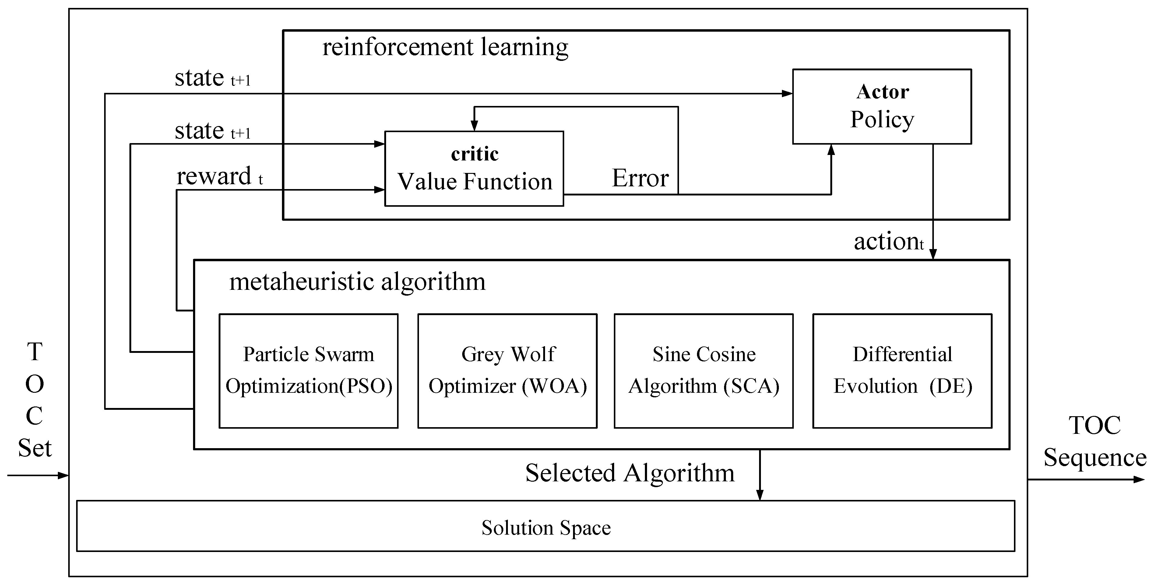
4.3. High-Level Algorithm Based on Actor–Critic Reinforcement Learning

(1)

Overview

Lower-level operators, by encompassing various initial uncertain states, necessitate the involvement of a “smart computing expert” at a higher level to assess the current environment and accordingly select an appropriate algorithm based on that environment and state. Once the algorithm is chosen, it is executed using the set parameters to activate the lower-level operators, a process that affects and modifies the current environment and state, prompting the subsequent selection of suitable operators based on the new conditions, and so forth. Thus, the essence of the entire algorithmic process depends critically on the “smart computing expert’s” ability to accurately select and implement the appropriate algorithms.

During the operator selection phase, it is essential to consider relevant design methodologies from reinforcement learning, such as methods for describing states, definitions of reward functions, criteria for action definition and selection, network architecture design, and other training and strategy designs.

Overall, the algorithm describes the spacecraft’s relevant resources and attributes as state features, utilizing the deep neural network to enhance the model’s parameterization and adaptability to complex and diverse environments. Moreover, action selection is based on the ε-Greedy Strategy, and dynamic reward functions are defined across four dimensions: global search capabilities, solution optimization quality, algorithm convergence speed, and types of applicable problems. This approach aims to differentiate reward functions in the early and late phases of training, thereby enhancing the model’s training effectiveness.

(2)

State

The design of the state significantly affects the computational accuracy of hyper-heuristic algorithms. In this study, we regard several solutions optimized by heuristic algorithms as part of the state, which are integrated with other elements (such as resource consumption, cost, and current resources) to form a comprehensive state representation matrix. According to Equation (16), the current solution matrix is denoted as $X$, thereby defining the state space $S$ as follows:

$$S=\left\{X,R,C,P,W\right\}$$

(28)

Here, resource information $R$ includes all details pertaining to the resources required for task execution $r_i^n$, the total available resources $R_{\mathrm{total} }^n$, and the resources accrued after completing tasks $e_{ij}^n$. Cost and benefit information $C$ encompasses the cost–benefit ratio $c_{ij}$ from task $i$ to task $j$ and the benefits obtained after completing task $j{V}_{ij}.P$ represents the threshold for the minimum cost–benefit ratio $P_{\mathrm{m}\mathrm{i}\mathrm{n}}$, and $W$ indicates whether time-related constraints are present.

Given the variations in dimensions and shapes of matrices formed by these constraints, methods such as normalization, padding, and feature extraction are necessary to process these matrices. This allows the extracted features to be input as a cohesive state into the model. Such processed state inputs enable the trained model to adapt to diverse tasks and constraints effectively.

(3)

Action selection

In this paper, the reinforcement learning algorithm is defined with an action set $A=$ $\left\{a_1,a_2,a_3,a_4\right\}$. The action set comprises four heuristic algorithm operators. Based on the current environmental conditions, the algorithm selects the appropriate operator (i.e., heuristic algorithm) and executes the corresponding code according to pre-set parameters.

During model training, the early action selection strategy has a significant impact on the performance of the algorithm since the initial probability distribution is random or directly specified. For instance, if high probability actions are consistently chosen early on, the algorithm may overly rely on these known optimal actions, thereby causing the model to converge on local optima as it struggles to explore more advantageous strategies.

The action selection strategy employed in this study is the $\epsilon$-Greedy Strategy, which effectively addresses the trade-off between exploration and exploitation. The basic strategy is as follows:

$$a_t=\left\{\begin{array}{ll}\mathrm{r}\mathrm{a}\mathrm{n}\mathrm{d}\mathrm{o}m\left(A\right)& \mathrm{if} \mathrm{random}\left(A\right)<ϵ\\ {\mathrm{a}\mathrm{r}\mathrm{g}\mathrm{m}\mathrm{a}\mathrm{x}}_a Q\left(s_t,a\right)& \mathrm{otherwise}\end{array}\right.$$

(29)

where $a_t$ is the action chosen at time $t$. The algorithm defines an exploration rate $ϵ$. If the result of $\mathrm{r}\mathrm{a}\mathrm{n}\mathrm{d}\mathrm{o}\mathrm{m}\left(\right)<ϵ$, the exploration mechanism is activated; otherwise, the action estimated to yield the highest expected reward is greedily selected, facilitating exploitation.

Regarding the adjustment of the exploration rate, given the instability of the initial probability distribution, a higher exploration rate is warranted initially. As training progresses to ensure stability in the decision-making process, the exploration rate should gradually decrease. The adjustment formula for the exploration rate is

$$ϵ\left(t\right)={ϵ}_{\mathrm{m}\mathrm{i}\mathrm{n}}+\left({ϵ}_{\mathrm{m}\mathrm{a}\mathrm{x}}-{ϵ}_{\mathrm{m}\mathrm{i}\mathrm{n}}\right)\times e^{-\lambda t}$$

(30)

Here, it is necessary to define the initial exploration rate ${ϵ}_{\mathrm{m}\mathrm{a}\mathrm{x}}$, the minimum exploration rate ${ϵ}_{\mathrm{m}\mathrm{i}\mathrm{n}}$, and the decay rate $\lambda .ϵ\left(t\right)$ represents the exploration rate at time $t$. Through this method, the exploration rate starts at a higher value and gradually decreases over time to a lower value.

(4)

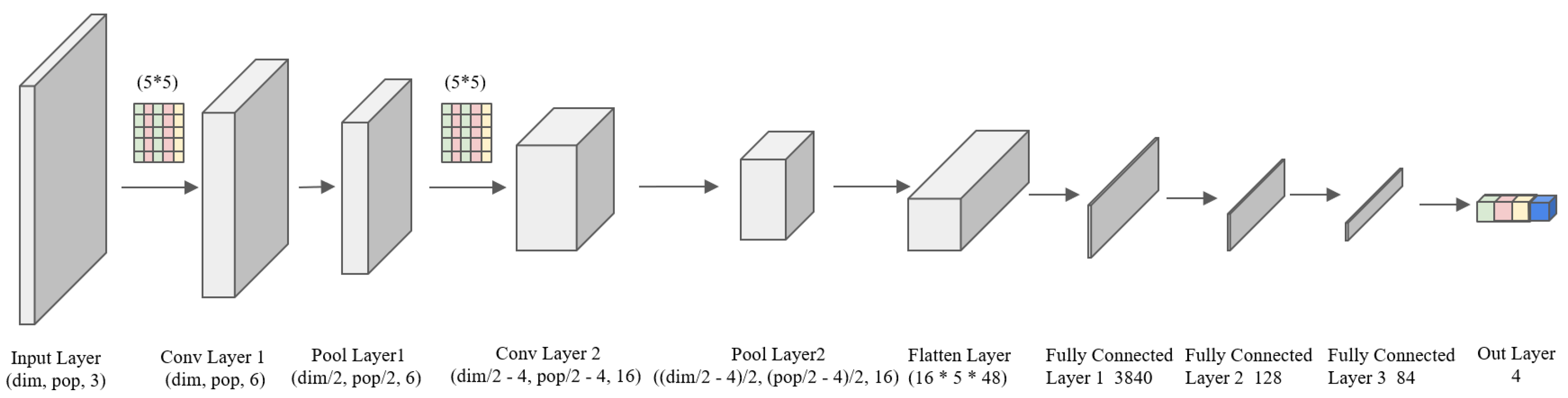
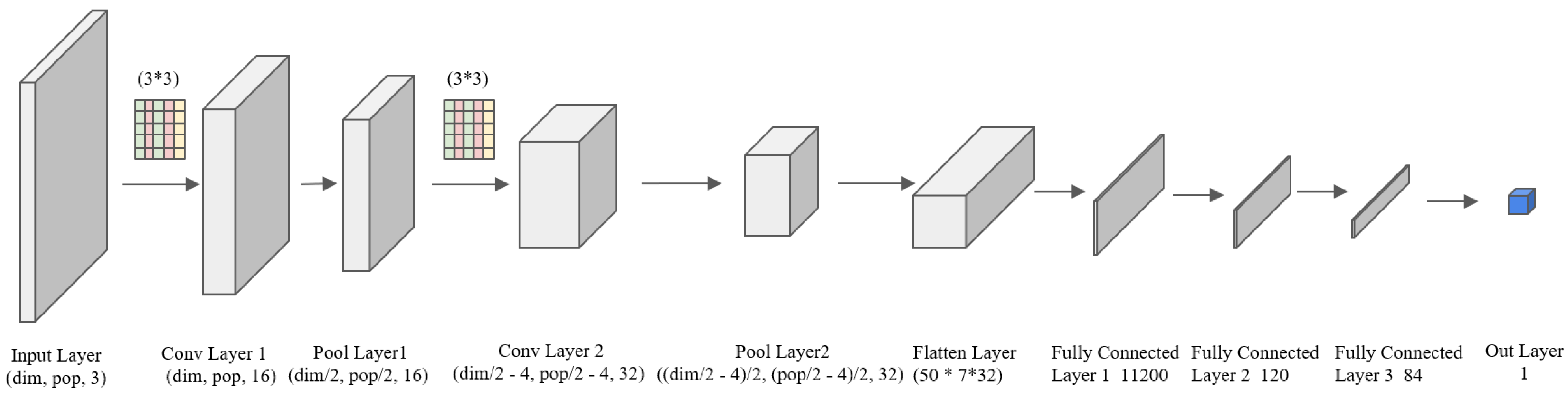
Actor–Critic network structure design

The actor–critic (AC) method is a sophisticated reinforcement learning algorithm that amalgamates the advantages of policy gradient methods with those of value function optimization techniques [66]. In the upper layer of our study’s algorithm, we have adopted this method as the primary reinforcement learning framework.

In this approach, there are two interconnected network structures: the actor network (Figure 3) and the critic network (Figure 4). The actor network (A) receives the state of the environment as input and outputs the probabilities of selecting each possible action. Its primary objective is to select actions based on the current policy, with the aim of maximizing expected rewards through policy learning. The critic network (C) also inputs the state of the environment but outputs an estimate of the current state’s value, assessing the value of states or state–action pairs by learning the value function of actions [67].

Initially, the actor network acts within the environment according to the current policy. Subsequently, the critic network evaluates the effectiveness of this action and computes the temporal difference (TD) error. The actor network then updates its strategy based on feedback from the critic network. Simultaneously, the critic network updates its estimate of the value function based on the TD error. The pseudo-code for the algorithm is provided in Algorithm 5.

Algorithm 5: Actor-Critic Based Metaheuristic Algorithm

Initialize policy network parameters ${\theta }^{\pi }$, value network parameters ${\theta }^v$ Initialize environment and state $s$ for each episode do     Reset environment and observe initial state $s$     while not done do           action $a$ according to the policy $\pi \left(a\mid s,{\theta }^{\pi }\right)$         Execute action $a$ in the environment                 Observe reward $r$ and new state $s^{\prime }$ Compute advantage estimate $A(s,a)=r+\gamma V\left(s^{\prime },{\theta }^v\right)-V\left(s,{\theta }^v\right)$ Update policy ${\theta }^{\pi }\leftarrow {\theta }^{\pi }+\alpha {\nabla }_{{\theta }^{\pi }}\mathrm{l}\mathrm{o}\mathrm{g}\pi \left(a\mid s,{\theta }^{\pi }\right)A(s,a)$ Update value ${\theta }^v\leftarrow {\theta }^v-\beta (r+\gamma V\left(s^{\prime },{\theta }^v\right)-V\left(s,{\theta }^v\right)){\nabla }_{{\theta }^v}V\left(s,{\theta }^v\right)$                                                                 $s\leftarrow s^{\prime }$             end while if end of evaluation period then Evaluate the policy end if end for

For the actor network, the action probability distribution is defined as follows:

$$\pi \left(a\mid S;{\theta }^{\pi }\right)=\left(1-ϵ\left(t\right)\right)\cdot \mathrm{s}\mathrm{o}\mathrm{f}\mathrm{t}\mathrm{m}\mathrm{a}\mathrm{x}\left(f^{\pi }\left(S;{\theta }^{\pi }\right)\right)+ϵ\left(t\right)\cdot {\displaystyle \frac{1}{\left|A\right|}}$$

(31)

Here, $a$ represents the action, $S$ is the state, and ${\theta }^{\pi }$ are the parameters of the actor network, with $f^{\pi }$ denoting its function. This formula delineates the probability of selecting action $a$ in state $S$. Initially, $f^{\pi }$ computes scores for all actions, which are subsequently converted into a probability distribution using the softmax function, ensuring that the sum of all action probabilities equals one and that the selection probability is positively correlated with the scores. Moreover, the exploration rate $ϵ\left(t\right)$ ensures a degree of random exploration.

In this study, we designed the architecture of the actor network, which tailored in our setting to output four operations (operators), with a complex input matrix (state $S$). The entire network consists of two convolutional layers, two pooling layers, and two fully connected layers, culminating in a Softmax output. The network architecture is illustrated as follows:

$$f^{\pi }\left(S;{\theta }^{\pi }\right)=\mathrm{Softmax}\left({\mathrm{F}\mathrm{C}}_2\left(\mathrm{Activation}\left({\mathrm{F}\mathrm{C}}_1\left({\mathrm{Pool}}_2\left({\mathrm{Conv}}_2\left({\mathrm{Pool}}_1\left({\mathrm{Conv}}_1\left(S\right)\right)\right)\right)\right)\right)\right)\right.$$

(32)

The loss function for the actor network is defined in two parts. The first part consists of the expected negative log probability multiplied by the action’s advantage function $A\left(s,a\right)$, aimed at guiding the policy to enhance reward values. The second part involves the entropy of the policy to encourage exploration of new actions, defined as

$$L\left({\theta }^{\pi }\right)=-{\mathbb{E}}_{\mathrm{S}\sim {\rho }^{\pi },a\sim \pi }\left[\log \pi \left(a\mid \mathrm{S};{\theta }^{\pi }\right)A\left(S,a\right)\right]+\beta H\left(\pi \left(\cdot \mid \mathrm{S};{\theta }^{\pi }\right)\right)$$

(33)

The network parameters ${\theta }^{\pi }$ are updated through gradient ascent. Here, $\beta$ is the coefficient for the entropy regularization term, and $H\left(\pi \left(\cdot \mid S;{\theta }^{\pi }\right)\right)$ represents the entropy of the policy. High entropy implies greater randomness in action selection. The advantage function $A\left(S,a\right)$ assesses the average merit in a given state $S$ and is defined as

$$A\left(S,a\right)=r+\gamma V\left(S^{\prime }\right)-V\left(S\right)$$

(34)

Here, $r$ is the immediate reward obtained after executing action $a,\gamma$ is the discount rate for future rewards, and $V\left(S^{\prime }\right)$ is the estimated value function for the next state $S^{\prime }$. This methodology allows for the approximation of the advantage function through the value function estimated by the critic network, simplifying the computation.

For the critic network, the value function is defined as

$$V\left(\mathrm{S};{\theta }^v\right)=f^v\left(\mathrm{S};{\theta }^v\right)$$

(35)

where ${\theta }^v$ are the parameters of the critic network, and $f^v$ is a function composed of two convolutional layers and three fully connected layers. This simplified network version is chosen due to the simplicity of the output from the policy function.

The loss function of the critic network calculates the error between the network’s value estimation and the actual rewards:

$$L\left({\theta }^v\right)={\mathbb{E}}_{s\sim {\rho }^{\pi }}\left[{\left(V\left(s;{\theta }^v\right)-R_t\right)}^2\right]$$

(36)

where $R_t$ is the actual return starting from state $s$. The network parameters ${\theta }^v$ are updated through gradient descent.

Based on the described methods, an adaptable actor–critic network can be constructed, providing ample justification for action selection.

(5)

Optimization Metrics

Before defining the reward function, it is essential to clarify the key performance metrics that the algorithm aims to improve, as the design of the reward function in high-level reinforcement learning is closely tied to these metrics. In this study, the defined optimization metrics are directly proportional to the level of improvement achieved; thus, higher improvements correspond to higher reward values. Consequently, the goal of the algorithm is to enhance these metrics by obtaining high reward values.

This research establishes four critical metrics: global search capability, quality of solution optimization, algorithm convergence speed, and applicability to problem types. For each metric, both stepwise and overall rewards must be considered within the reward function.

Global search index $\left(\Delta \right)$: The Global Search Index is a metric used to quantify the diversity of solutions in heuristic algorithms by evaluating the ratio of distinct solutions generated during a specified iteration period to the theoretical maximum number of possible solutions. This metric reflects the algorithm’s ability to explore the search space globally, indicating how well it maintains diversity throughout the search process. The mathematical expression is

$${\Delta }_{\mathrm{global} }={\displaystyle \frac{N_{\mathrm{unique} }}{I\times S}}$$

(37)

where $N_{\mathrm{unique} }$ denotes the number of distinct solutions, $I$ represents the number of iterations, and $S$ indicates the size of the solution space.

Quality of solution optimization ($\eta$): This metric assesses the improvement of a solution compared to the initial state. The stepwise reward is defined below:

$${\eta }_{\mathrm{quality}}=1-{\displaystyle \frac{\mathrm{P}\left(X\right)}{{\mathrm{P}}_{\mathrm{prev}}\left(X\right)}}$$

(38)

where P(X) is the path length of the current solution $X$. The overall reward is calculated based on the specific improvement over the initial solution.

$$\left(\eta \right)=\mathrm{P}\left(X_{\mathrm{before} }\right)-\mathrm{P}\left(X_{\mathrm{after} }\right)$$

(39)

Weighted Convergence Speed $(\tau$): This metric quantifies the average number of steps required for the algorithm to converge to the current optimal solution. It measures the speed and stability of the algorithm by assigning a weight to each adaptation improvement.

$$\tau ={\displaystyle \frac{\sum _{i=1}^I{w}_i\cdot \Delta f_i}{\mathrm{I}}}$$

(40)

Here, $w_i$ is the weight of the i-th adaptation improvement, set according to the actual situation. $\Delta f_i$ is the improvement value of adaptation after the ith iteration. Iteration is the total number of iterations required to reach the highest adaptation value.

With these metrics, an algorithm that reaches a high level of adaptation quickly in the early stages and then remains unchanged will receive a higher $\mathit{\tau }$ value because the weighting of reaching a high level of adaptation quickly in the early stages is greater. Additionally, if the algorithm is still making small improvements as it approaches its final fitness, these improvements, although small, will be factored into the overall evaluation, although they will not significantly affect the evaluation metrics.

Algorithm Composite Evaluation Index ($\xi$): This metric aims to quantify the average performance of the algorithm. For algorithms, surely the algorithm that achieves the best fitness is the most superior algorithm. However, in aerospace, the real-time and optimization efficiency of the algorithm needs to be considered so that the algorithm can achieve the best possible results in as short a time as possible, while ensuring adequate coverage of the number of solutions, and still achieve a good degree of fitness. Combining the above needs, this study defines the Algorithm Composite Evaluation Index, which is used to combine the above three metrics to comprehensively evaluate the performance of an algorithm so that it can be applied to the specific field of aerospace and related scenarios.

The index is used to compare the combined performance of the above three metrics between multiple algorithms and in the same case, so multiple algorithms need to calculate the index at the same time in order to be comparable. A higher index indicates that the algorithm performed relatively better (i.e., converged faster and produced better results) in that instance. The specific calculation method of the index is as follows:

$$\xi =\sqrt[3]{w_1\left({\displaystyle \frac{\tau }{{\tau }_{max}}}\right)+{\left({\mathrm{w}}_2\cdot e^{0.01\cdot \left({\eta }_{max}-\eta \right)}\right)}^{{\displaystyle \frac{1}{3}}}+w_3\cdot \Delta }$$

(41)

In the above formula, ${\tau }_{max}$ and ${\eta }_{max}$ refer to the optimal value of the corresponding metrics in the algorithm in the same period, and the rest of the relevant participation is used for the metrics’ normalization. According to the importance ranking of the above three metrics, in this study we define $w_1:w_2:w_3=3:5:2$, i.e., the algorithm’s fitness is calculated to be the most important, followed by the speed of convergence, and lastly, the extent of the algorithm’s coverage of the solution. The following text study completes the comprehensive evaluation of the algorithm based on this metric.

(6)

Reward

In this study, the designed algorithm aims to meet the flexibility requirements in diverse environments, thus imposing stringent demands on maintaining consistent performance under various conditions. The selection of the four underlying algorithms must possess significant advantages to ensure the efficiency and effectiveness of the overarching meta-heuristic algorithm. Initially, the goal is to surpass the performance of individual algorithms through optimization based on a relative evaluation of higher-level decisions. As training progresses, the model theoretically should select the optimal solution that exceeds the performance of each standalone algorithm, rendering simple relative evaluations inadequate. Hence, it is necessary to assess the merits and demerits of algorithms and decisions from an absolute perspective to guide the training direction.

Consequently, the reward function in this research is divided into two main parts: the absolute factor $R_{\mathrm{absolute} }$ and the relative factor $R_{\mathrm{relative} }$. As training time increases and training effects improve, the proportion of the absolute factor gradually increases, while that of the relative factor correspondingly decreases. The expression is given by

$$R\left(t\right)=\left({\displaystyle \frac{1}{1+e^{-k\left(t-t_0\right)}}}\right)\cdot R_{\mathrm{absolute}}\left(\mathrm{t}\right)+\left(1-\left({\displaystyle \frac{1}{1+e^{-k\left(t-t_0\right)}}}\right)\right)\cdot R_{\mathrm{relative}}$$

(42)

where $t_0$ is the point in time when $\alpha$ and $\beta$ are equal.

In the reward function, the metrics are the four optimization indicators previously mentioned, calculated differently depending on whether the perspective is absolute or relative. For the absolute factor, the focus is on the absolute values of the optimization metrics and the changes before and after algorithm implementation. The formula is as follows:

$$R_{\mathrm{absolute}}\left(t\right)=\sum _i w_i\sum _{k=0}^{T-t} {\gamma }^k{\tilde{R}}_{i}t$$

(43)

Here, $R_{\mathrm{step} ,i}\left(t\right)$ and $R_{\mathrm{global}, i}$ represent the normalized step reward and global reward at time $t$ for metric $i$, respectively, with $w_i$ being the weight of metric $i$, and ${\sum }_i w_i=1.T$ is the total number of iterations, and $\gamma$ is the discount factor, used to adjust the weight of future rewards. The set of metrics includes $i\in \Delta ,\eta ,\tau ,\xi$.

For the relative factor, it is only necessary to compare the rankings of the meta-heuristic algorithm against the other four standalone heuristic algorithms. The higher the ranking of a corresponding metric, the greater the reward obtained. To encourage higher rewards, it is stipulated that higher rankings result in exponentially increasing rewards, as specified in the relative reward $R_{\mathrm{relative:} }$:

$$R_{\mathit{relative}}=r\sum _{i\in \Delta ,\eta ,\tau ,\xi } w_i\cdot e^{\left(N+1-{\mathit{rank}}_i\right)}$$

(44)

Here, ${\mathrm{r}\mathrm{a}\mathrm{n}\mathrm{k}}_i$ is the ranking position of the algorithm, $N$ is the total number of algorithms. $r$ is the raw reward value obtained through the optimization indicators associated with the absolute factor. Each metric $i$ has an assigned weight and ranking.

After integrating both absolute and relative factors, the training of the algorithm focuses on surpassing the performance of individual underlying algorithms and striving for better solutions, thereby enhancing the overall performance while optimizing the four specified metrics.

(7)

Training strategy

Building upon the aforementioned description, this study further incorporates the following training strategies. Firstly, a dynamic learning rate adjustment is utilized. Within the optimizer, the learning rate, $\eta$, is updated after each epoch via a scheduler according to the formula

$${\eta }_{t+1}={\eta }_t\cdot {\gamma }^{\lambda }$$

(45)

Here, ${\eta }_{t+1}$ represents the learning rate for the upcoming epoch, ${\eta }_t$ is the learning rate of the current epoch, $\gamma$ is a decay rate (typically less than 1), and $\lambda$ controls the rate of decrease in the learning rate. By progressively reducing the learning rate, the algorithm can converge more effectively, while also minimizing parameter fluctuations and overfitting in the later stages of training. An exponential decay strategy is employed to adjust the learning rate.

Secondly, for the actor and critic networks, the Adam optimizer is employed:

$${\theta }_{t+1}={\theta }_t-\eta \cdot {\displaystyle \frac{m_t}{\left(\sqrt{v_t}+ϵ\right)}}$$

(46)

where $\theta$ denotes the network parameters, $\eta$ is the learning rate, $m_t$ is the bias-corrected estimate of the first-order momentum, $v_t$ is the bias-corrected estimate of the second-order momentum, and $ϵ$ is a small constant added to ensure numerical stability. The Adam optimizer is utilized to adjust model parameters, allowing for the adaptive adjustment of learning rates for each parameter.

5. Experiment

To validate the effectiveness and performance of the proposed algorithm in real-world environments, this study has designed several sets of experiments. Initially, the validity and training process of the model are analyzed by examining changes in the reward function values and anticipated model changes through the training procedure. Subsequently, by integrating the four operators at the base of the hyper-heuristic algorithm, the effectiveness of the higher-level algorithm in selecting these operators is assessed. Finally, by comparing with other heuristic algorithms and common algorithms, the comprehensive effectiveness of this algorithm on relevant evaluation metrics against other operators and algorithms is verified.

5.1. Parameter and Environment Settings

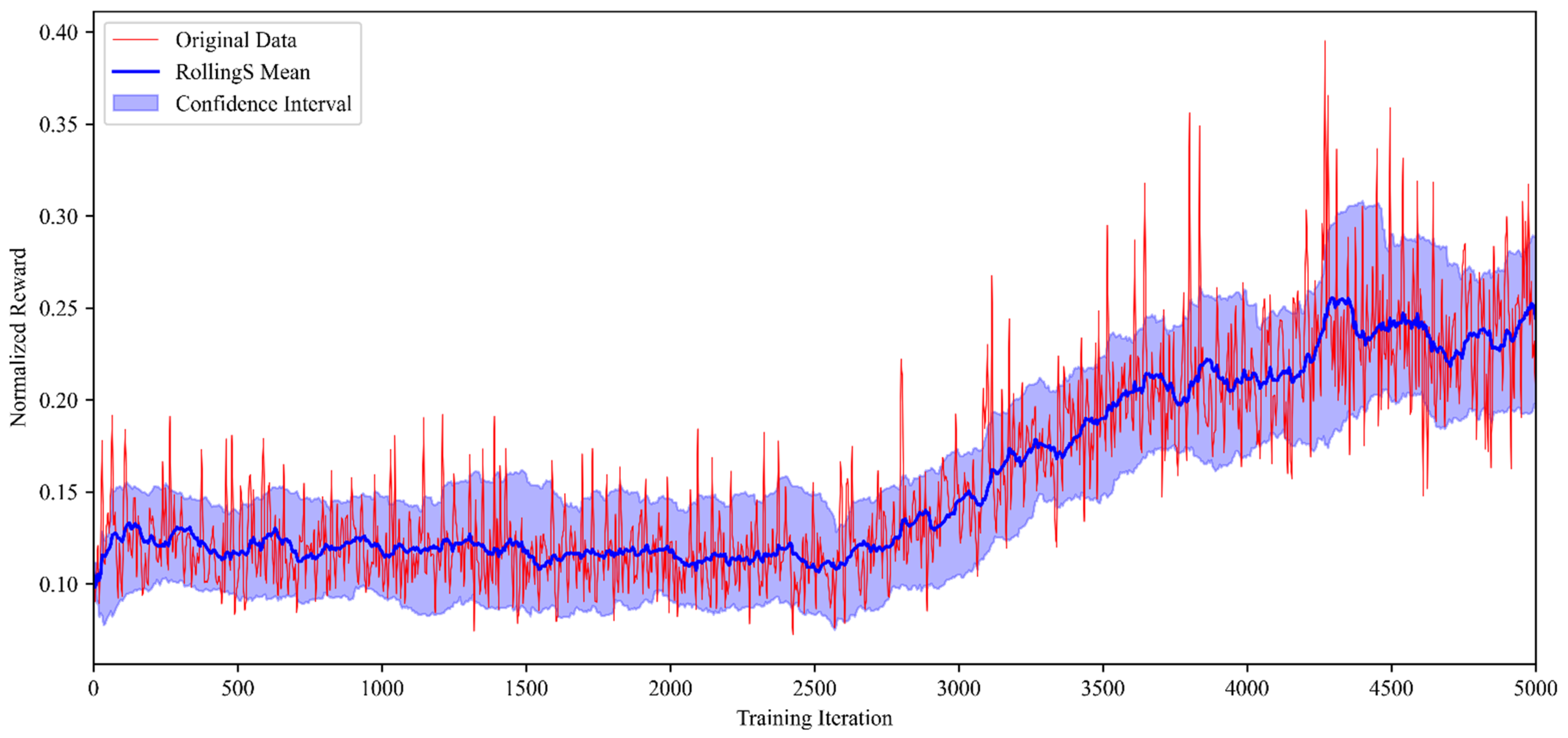
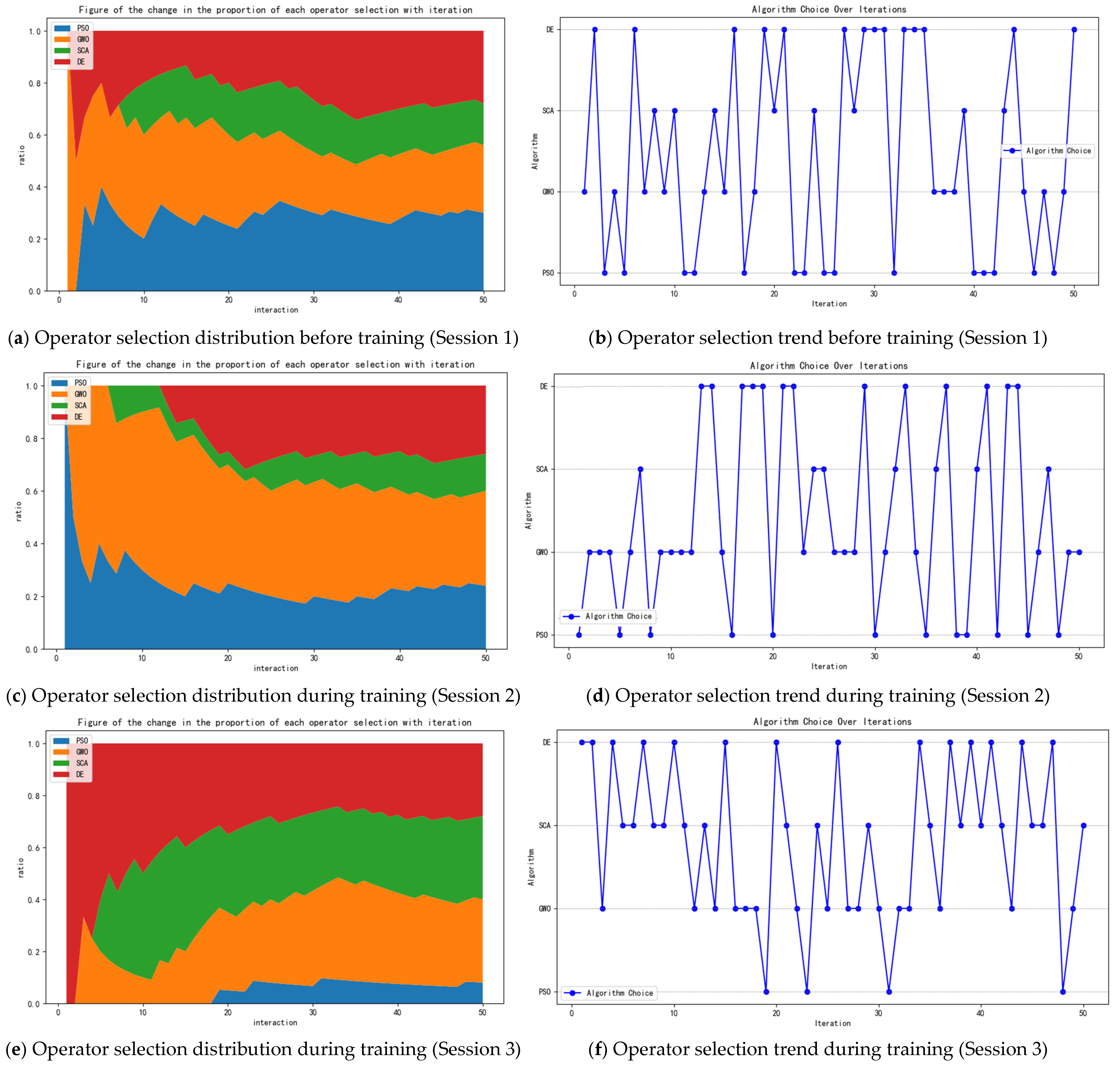
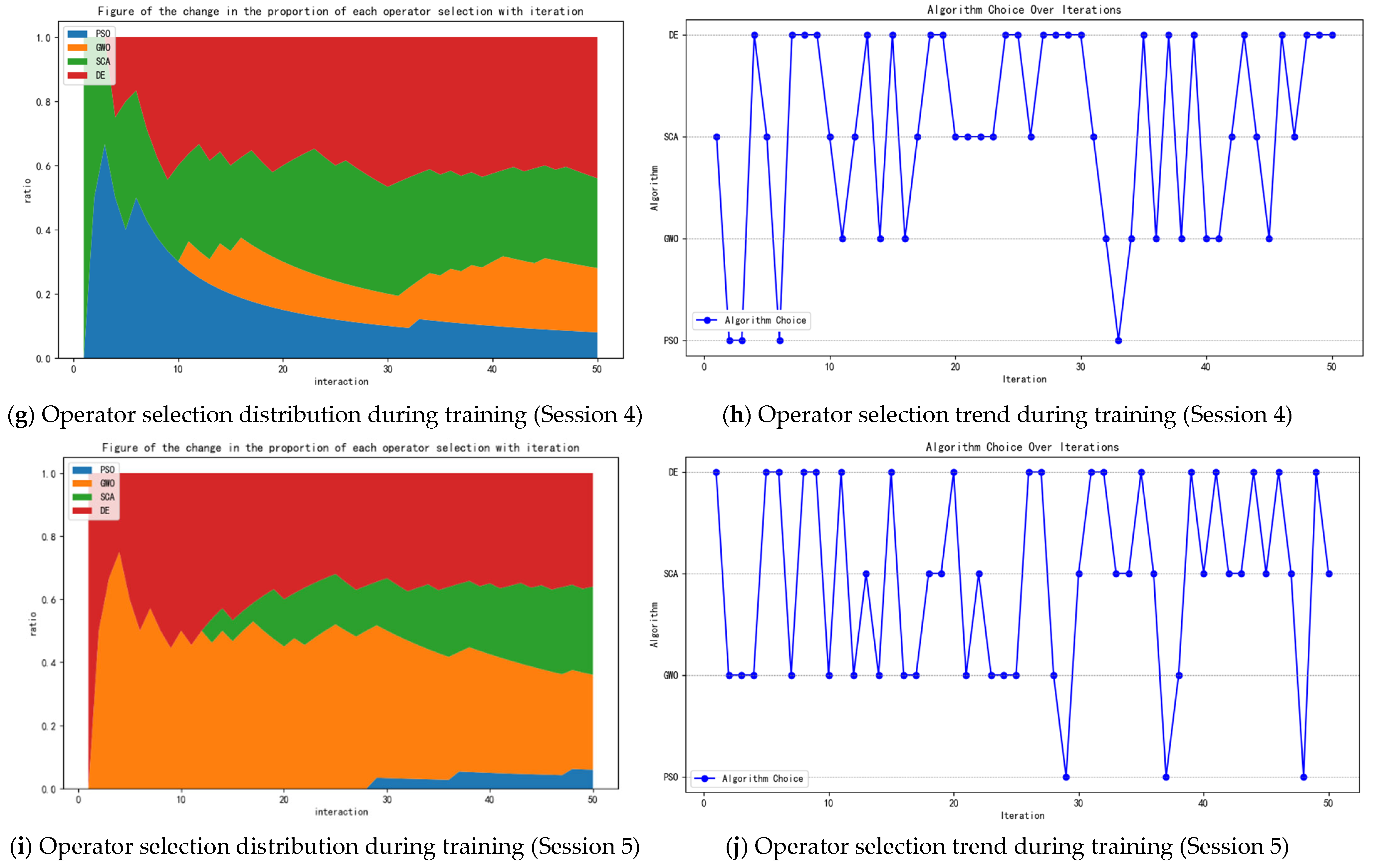
Due to the unique nature of this problem, there are no standard datasets available for testing. Therefore, the datasets used in this paper consist of task instances randomly generated according to the actual engineering requirements. We define two parameters for the spacecraft mission objectives with value ranges of (0,100), and the spacecraft’s initial position and state are set as default values. Subsequently, based on the task sequence, the spacecraft calculates and generates an optimized command sequence. The relevant parameters for the instances are defined in the following

Table 5. Environment parameters settings.

Property	Value
Spatial Range	(0,0) to (100,100)
Spacecraft Position Range	(0,0) to (100,100)
Max TOC Capacity	100
Number of Generated TOCs	(0,100)

.

In the proposed hyper-heuristic algorithm, the determination of relevant parameters influences the algorithm’s performance. Based on multiple previous tests and taking into account the experience from related research, we have identified the relevant parameters for the high-level aspects of the hyper-heuristic algorithm and the parameters for the lower-level operators. These parameters are shown in the

Table 6. Hyper-heuristic algorithm and low-level operator parameters.

Object	Property	Value
RL strategy	Action Dimension	4
	Actor Learning Rate	2 × 10−4
	Critic Learning Rate	3 × 10−3
	Hidden Dimension	120
	Discount Factor (γ)	0.95
	Entropy Beta	0.05
	Epsilon Start	1.5
	Epsilon End	0.01
	Epsilon Decay	500
	Num Episodes	10,000
	Optimizer	Adam
	Actor Scheduler Gamma	0.9
	Critic Scheduler Gamma	0.9
SCA	scale	200
	Growth Rate	0.1
	Competition Rate	0.1–0.25
	Iterations	1000
PSO	scale	200
	C1	2.0
	C2	1.0
	W	Typically between 0.5 and 1.0
	Velocity	−0.2–0.2
	Iterations	1000
	w	0.9
DE	scale	200
	Differential Weight	0.5
	Crossover Probability	0.9
	Iterations	1000
GWO	scale	200
	A	Linearly decreasing from 2 to 0 |
	C	Random values between 0 and 2
	Iterations	1000

.

In this study, all algorithms were coded using Pytorch 2.0.0 and Python 3.9.18, and implemented on a personal computer with an Intel(R) Core(TM) Ultra 5 125 H processor (manufactured by Intel Corporation, Santa Clara, CA, USA)running at 1.2 GHz with 32 GB RAM for training and principle testing. During the training process, CUDA and an NVIDIA GeForce RTX 4060 Laptop GPU (manufactured by Intel Corporation, Santa Clara, CA, USA)were used for computational acceleration.

5.2. Model Training

In this study, the training scenario is as follows: the task parameters are defined based on a TOC command structure, where each task (TOC) represents a motion planning action for a gimbal system, characterized by two key parameters: Azimuth (horizontal direction, ranging from 0 to 180 degrees) and Elevation (vertical direction, ranging from 0 to 180 degrees). Task instances are generated according to the rules in Table 4, producing between 30 and 70 TOCs, with parameters such as time window, resource consumption, and resource replenishment randomly set within reasonable ranges. For example, the time window is set to 0 or 1 to simulate task timing constraints, and resource consumption is uniformly distributed to ensure that the total consumption does not exceed the resource limit. The environment simulation assumes that both the spacecraft and target positions are randomly distributed within a two-dimensional space, ranging from (0,0) to (100,100).

The training process of the model described in this study was based on CUDA and utilized the aforementioned GPU acceleration. During training, the algorithm’s reward function was defined in accordance with the earlier discussion on rewards, and continuous monitoring and recording were conducted. The study carried out 20 training sessions, each with a sufficient number of iterations. The trend graphs of the average, upper, and lower bounds of the reward function during these trainings are shown in Figure 5.

Here, the red fold represents the reward function change for one of the training sessions, the blue finding fold represents the average value of the reward function change, and the blue fill represents the sliding window of the highest and lowest values of the reward function change over the course of the multiple testing sessions described above. The value on the red fold represents the specific value of the reward function that can be obtained based on the algorithm completing one planning at the current number of iterations.

According to the above figure, it can be seen that the reward function score is low in the initial phase of the algorithm. Afterwards, the reward obtained gradually increases as the training progressively deepens. At the same time, the hyper-heuristic algorithm gradually outperforms the four underlying heuristics alone and obtains higher scores. The reward values fluctuate slightly due to the change in the reward function during the training iterations, which causes the algorithm to favor the global rather than outperform the individual four algorithms, although it ultimately stays within an interval. Comprehensively, the above figure reflects that the change in reward value will gradually improve, thus proving that the reinforcement learning algorithm can effectively improve the evaluation results of the relevant indicators, proving the effectiveness of the algorithm.

Meanwhile, during the training process, the selection scheme for the four underlying algorithms at each training is recorded. Figure 6 shows the stacked area plot of the proportion of the number of times the selection tendency was made for each of the four times during the training iteration cycle, initially and after the end of the model training, respectively.

Observing the above figure, we can find that the first two figures are the distribution of the model’s action selection before training. We can find that, before training, the model’s choices tend to be random, and the distribution of each action is basically equal. After the completion of multiple rounds of training, the last eight graphs show four times the model’s choice of operators at runtime. It can be noticed that the choice of operators has been differentiated due to the differences in the problems. For example, for Figure 6c,d, the tendency is to use the grey wolf optimization algorithm and the particle swarm algorithm to speed up the iterations at the beginning of the computation, while for Figure 6e–h, the tendency is to use the differential evolution algorithm to iterate quickly. Figure 6i,j, on the other hand, would use GWO and DE to speed up the iterations in the early stages, but used the PSO algorithm a number of times in the later stages to try to obtain more solutions. This illustrates the algorithm’s ability to target the right operators to achieve better results when faced with different particle states.

5.3. Comparative Experiments with AC-HATP and Operators

To validate the optimization performance of the algorithm, this section of the experiment first compares the algorithm implemented in this study with four underlying operators against relevant optimization metrics, to demonstrate the degree of optimization in the actual results by high-level selection, as well as the extent to which the advantages and disadvantages of several algorithms are combined.

Firstly, we compare the optimal fitness of optimization. In the

Table 7. Values of the fitness function for the four underlying operators and the algorithm of this paper tested in 16 instances.

Instance ID	Number of Tasks in Instance	PSO			GWO			SCA			DE			AC-HATP
		Avg.	Min.	Std.	Avg.	Min.	Std.	Avg.	Min.	Std.	Avg.	Min.	Std.	Avg.	Min.	Std.
Task Case1	10	195	193	4.73	200	193	7.34	195	193	4.29	193	193	0.68	193	193	0.72
Task Case2	14	270	244	12.07	266	244	16.12	266	244	15.36	269	244	8.99	264	244	9.13
Task Case3	18	321	292	23.91	321	292	23.19	350	304	28.4	299	292	1.98	298	292	3.25
Task Case4	22	471	407	45.64	448	403	37.57	542	489	36.1	403	383	9.08	403	383	12.06
Task Case5	26	563	421	70.76	494	410	52.89	662	558	53.08	416	387	15.1	410	387	20.06
Task Case6	30	605	506	56.49	535	450	61.25	755	676	45.73	436	412	33.38	439	415	35.25
Task Case7	34	731	564	134.9	586	440	90.93	1055	859	98.83	428	411	24.67	425	411	41.12
Task Case8	38	900	679	141.33	715	592	89.13	1227	995	88.89	588	499	56.88	593	499	72.23
Task Case9	42	1017	774	145.88	769	570	98.64	1277	1077	86.11	630	534	63.84	616	532	75.86
Task Case10	46	1224	931	232.78	948	707	175.21	1582	1468	72.1	706	640	90.3	701	633	102.5
Task Case11	50	1264	1038	144.3	887	597	144.49	1654	1481	99.79	689	591	69.22	655	584	80.36
Task Case12	54	1654	1099	287.04	1235	785	340.97	1938	1765	87.5	879	709	123.98	863	702	159.56
Task Case13	58	1815	1370	260.31	1143	891	133.38	2099	1931	91.08	959	768	136.3	933	745	122.5
Task Case14	62	2207	1670	289.41	1431	982	347.48	2446	2267	95.82	1172	949	131.4	1103	932	153.2
Task Case15	66	1930	1545	201.28	1191	745	367.68	2220	2045	72.18	1190	999	134.94	1186	993	155.36
Task Case16	70	2320	1629	245.54	1505	1126	251.42	2549	2349	87.79	1424	1068	178.04	1385	1033	186.46

below, each instance corresponds to a set of tasks, and the number of tasks per instance can be obtained from the table. Each set of instances underwent 20 experiments, with the results indicating the final fitness value of the current experiment. We filled the average, minimum values, and standard deviations into the table. The minimum value allows for an observation of the lowest fitness that the algorithm can achieve, reflecting the algorithm’s optimal performance, although this does not represent the overall level of the algorithm. The average value reflects the average convergence time of the entire algorithm, representing the overall level of the algorithm. The standard deviation indicates the stability of the algorithm; a smaller standard deviation means that the solutions obtained by the algorithm are more stable.

By examining the table, it can be observed that, in terms of final fitness, the GWO and DE algorithms perform similarly to AC-HATP, all achieving good convergence results. PSO and SCA, however, show slightly inferior performance in terms of fitness. Additionally, in most instances, AC-HATP performs slightly better than DE, with specific instances showing AC-HATP’s optimal fitness performance significantly stronger than both GWO and DE (for example, Task Case 13 and Task Case 16). However, there are instances wherein DE’s optimal fitness surpasses the algorithm presented in this paper (such as Task Case 6). Also, the standard deviation of this paper’s algorithm is slightly larger than that of DE, suggesting the potential to achieve superior solutions in some cases. This result confirms that AC-HATP can address the issue wherein GWO, despite its fast convergence speed, may only find local optima in certain cases and can also harness the advantages of the differential evolution algorithm to achieve superior solutions. That is, AC-HATP can integrate additional features from other algorithms to achieve overall superior fitness performance.

Next, a comparison of the convergence time of the underlying operators and the algorithm of this paper is presented. In the

Table 8. Weighted convergence speed (WCS) of the four underlying operators and the algorithm of this paper tested in 16 instances.

Instance ID	Number of Tasks in Instance	PSO			GWO			SCA			DE			AC-HATP
		Avg.	Max.	Std.	Avg.	Max.	Std.	Avg.	Max.	Std.	Avg.	Max.	Std.	Avg.	Max.	Std.
Task Case1	10	0.0001	0.0002	0.0001	0.0078	18.7091	0.2149	0.0056	15.6761	0.1553	0.0098	13.0767	0.2322	0.0104	17.1645	0.4554
Task Case2	14	0.0003	0.0005	0.0001	0.0324	46.7765	0.8429	0.0169	46.1657	0.4844	0.0282	50.8921	0.6474	0.0366	48.3744	0.2364
Task Case3	18	0.0001	0.0002	0.0001	0.0243	25.1133	0.567	0.0207	31.5107	0.546	0.0233	32.6495	0.4282	0.0225	36.6633	0.3665
Task Case4	22	0.0008	0.001	0.0003	0.0363	62.1455	0.927	0.0178	26.4711	0.3928	0.0317	34.2578	0.6099	0.0324	45.5843	0.5364
Task Case5	26	0.0007	0.0009	0.0002	0.0296	69.4211	0.8448	0.0255	49.6433	0.744	0.0481	72.3222	1.0356	0.0368	63.331	0.8223
Task Case6	30	0.0002	0.0003	0.0001	0.0349	58.9927	0.8913	0.0158	30.0202	0.3971	0.043	47.6987	0.7876	0.0361	62.3372	0.5746
Task Case7	34	0.0003	0.0004	0.0001	0.047	64.098	1.0587	0.0293	48.1168	0.8451	0.0599	113.4906	1.3527	0.0511	72.2661	0.3661
Task Case8	38	0.0005	0.0007	0.0002	0.0343	37.8841	0.7375	0.0247	84.3945	0.8828	0.0435	69.839	0.8695	0.0395	56.1353	0.4366
Task Case9	42	0.0007	0.0008	0.0003	0.0327	88.3789	1.0344	0.0294	58.6144	0.7744	0.045	54.0082	0.8037	0.0438	56.6332	0.8735
Task Case10	46	0.0003	0.0005	0.0001	0.0445	86.4128	1.1192	0.0281	41.1967	0.691	0.0568	97.9028	1.3335	0.0633	75.4003	0.8614
Task Case11	50	0.0001	0.0002	0.0001	0.0335	49.1717	0.8569	0.038	87.688	1.2255	0.0528	52.0891	0.96	0.0462	69.4387	0.6339
Task Case12	54	0.0003	0.0005	0.0001	0.0285	44.1303	0.7858	0.0359	84.1254	1.1072	0.0433	80.951	1.0153	0.0458	76.6436	0.7268
Task Case13	58	0.0005	0.0007	0.0002	0.0421	77.9441	1.1603	0.0333	74.6741	0.9905	0.0564	84.4854	1.3202	0.0495	86.6395	0.5244
Task Case14	62	0.0006	0.0007	0.0003	0.034	78.1847	1.0699	0.0328	73.4801	0.9486	0.0463	74.291	1.0593	0.0497	72.3664	0.7353
Task Case15	66	0.0002	0.0003	0.0001	0.0412	80.9367	1.1975	0.0288	55.8044	0.802	0.0372	46.2811	0.6629	0.0447	96.1353	0.9562
Task Case16	70	0.0004	0.0005	0.0002	0.0345	65.941	0.8935	0.0395	104.4515	1.3269	0.0469	50.9532	0.9381	0.0489	72.1054	1.0254

below, each set of instances underwent 20 experiments, with the results reflecting the convergence time defined in the aforementioned metrics. We filled in the average, minimum values, and standard deviations into the table. The minimum value allows for an observation of the smallest values achieved by the algorithm, the average value reflects the overall average convergence time of the algorithm, and the standard deviation indicates the stability of the algorithm, with a smaller standard deviation implying greater stability.

By observing the table, it can be found that PSO generally struggles to achieve faster convergence speeds, while DE and AC-HATP can achieve better convergence speeds, significantly outperforming other algorithms. Additionally, the overall convergence speed of AC-HATP is superior to both DE and GWO. SCA has slower convergence speeds, although it can also achieve relatively fast convergences in some cases. Overall, the convergence speed of the algorithm designed in this study is superior to that of the other operators.

We have selected Task Case 8 from several test runs to plot the convergence curves of the algorithm, as shown in Figure 7.

Combining the above figures, it can be seen that the algorithm designed in this study achieves a fast convergence speed in the initial stages, and the final convergence results are maintained at a good level. Considering the practical engineering requirements of aerospace, the algorithm needs to obtain superior solutions in a short period of time, which demonstrates that the algorithm designed in this study can support practical applications.

Next, a comparison of the diversity of solutions between the underlying operators and the algorithm of this study is conducted. In the

Table 9. Diversity indices of solutions tested by the four underlying operators and the algorithm of this paper in 16 instances.

Instance ID	Number of Tasks in Instance	PSO-Avg.	GWO-Avg.	SCA-Avg.	DE-Avg.	AC-HATP-Avg.
Task Case1	10	0.0502	0.1141	0.302	0.0057	0.1336
Task Case2	14	0.1834	0.3873	0.7741	0.0078	0.1845
Task Case3	18	0.8787	0.5562	0.877	0.0152	0.2259
Task Case4	22	0.898	0.6594	0.9249	0.0188	0.2746
Task Case5	26	0.9926	0.773	0.9449	0.0232	0.3103
Task Case6	30	1	0.8372	0.9586	0.0271	0.3065
Task Case7	34	1	0.8662	0.9709	0.032	0.3564
Task Case8	38	1	0.8814	0.9765	0.0262	0.3362
Task Case9	42	1	0.9149	0.9812	0.0279	0.3523
Task Case10	46	1	0.9407	0.9844	0.0303	0.3198
Task Case11	50	1	0.9602	0.9881	0.0315	0.3664
Task Case12	54	1	0.9577	0.99	0.0293	0.3342
Task Case13	58	1	0.9631	0.991	0.0295	0.3462
Task Case14	62	1	0.9681	0.9925	0.0289	0.3321
Task Case15	66	1	0.982	0.9935	0.0262	0.3558
Task Case16	70	1	0.9794	0.9946	0.0255	0.3226

below, each set of instances underwent 20 experiments, with the results reflecting the diversity index of solutions (ranging from 0 to 1) as defined in the previous metrics. We filled the average values into the Table 9.

By observing the table, it can be seen that PSO and SCA generally achieve a sufficient number of solutions, while GWO and DE obtain a limited number of solutions. This is also why these two algorithms are prone to falling into local optima. AC-HATP also manages to obtain a considerable number of solutions, but overall fewer than PSO and SCA.

From the above comparisons, we can draw the conclusion. The AC-HATP algorithm designed in this study achieves fitness levels almost as excellent as DE, and its diversity of solutions is higher than DE, making it less likely to fall into local optima traps and more capable of obtaining superior solutions in various complex and diverse scenarios. Additionally, AC-HATP boasts excellent convergence time, achieving convergence in a shorter period. Therefore, AC-HATP combines the strengths of the four underlying operators, and overall, it is able to obtain superior solutions in a shorter time while maintaining diversity. These experiments also fully demonstrate the effectiveness of high-level reinforcement learning algorithms in operator selection.

5.4. Comparative Experiments with Other Algorithms

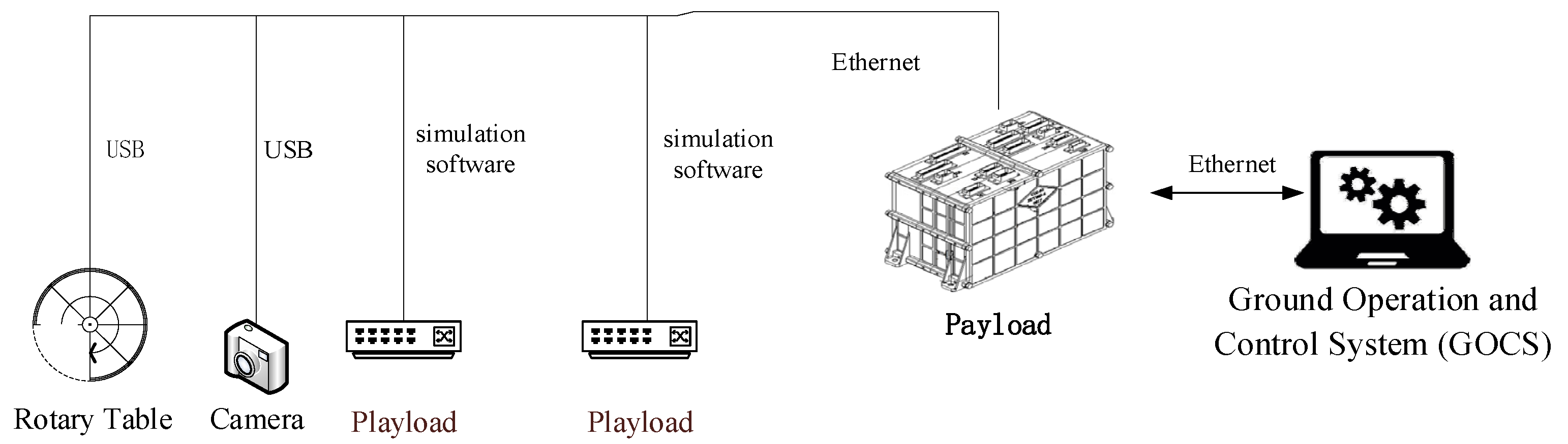
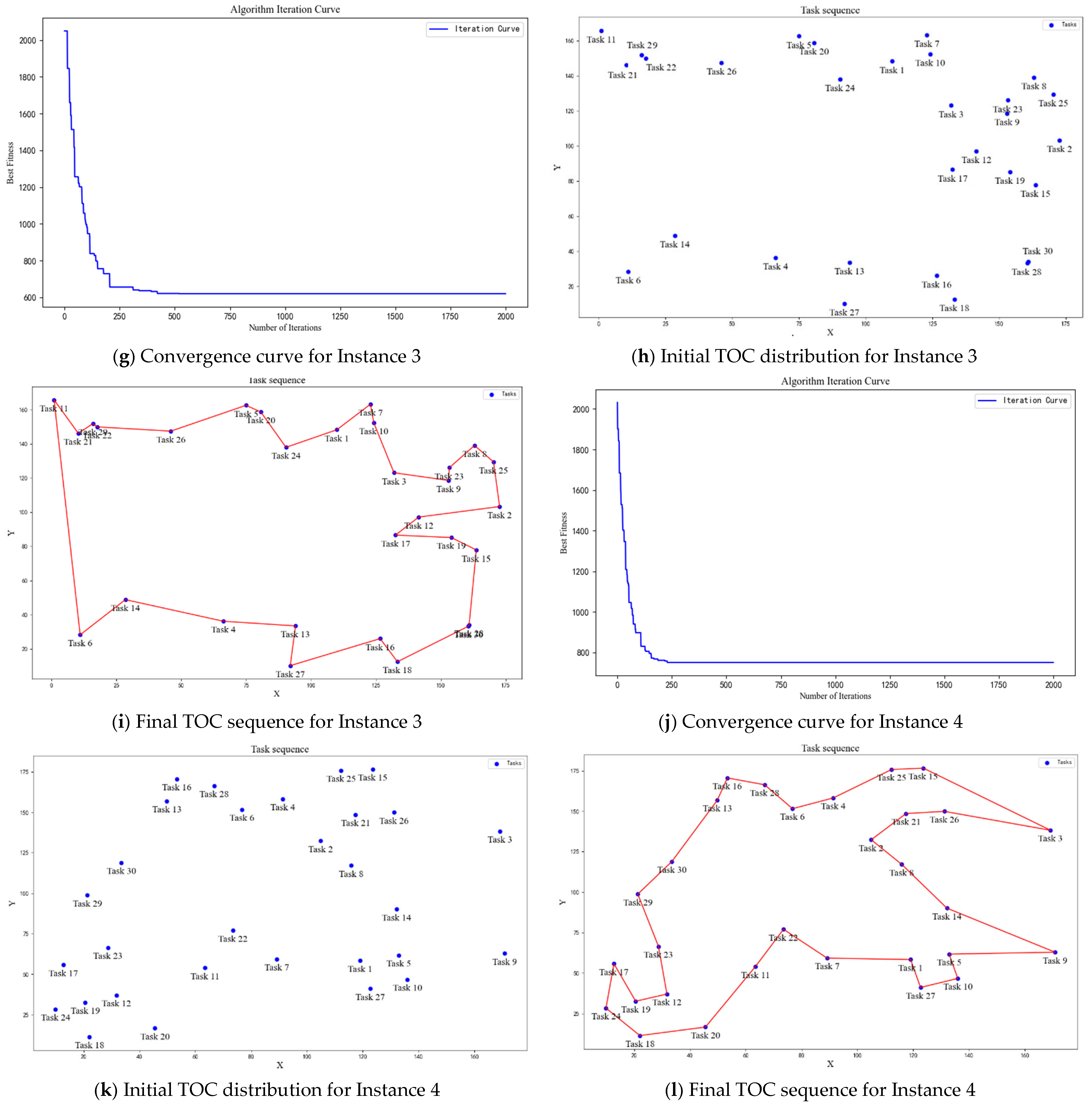
To enhance the credibility of this algorithm and its overall level under various conditions, this study selected two heuristic algorithms, two meta-heuristic algorithms, and two reinforcement learning-based hyper-heuristic algorithms [68,69] to compare with the algorithm presented in this paper.

The comparison table for optimal fitness is shown in the table below. In the

Table 10. Fitness function values of the six algorithms and the algorithm in this paper tested in 16 instances.

Instance ID	Number of Tasks in Instance	GA			SA			WDO			TSA			DMAB			SLMAB			AC-HATP
		Avg.	Min.	Std.	Avg.	Min.	Std.	Avg.	Min.	Std.	Avg.	Min.	Std.	Avg.	Min.	Std.	Avg.	Min.	Std.	Avg.	Min.	Std.
Task Case1	10	227	204	9.03	196	193	3.57	222	203	9.7	214	204	1.12	193	193	0.85	193	193	0.80	193	193	0.72
Task Case2	14	401	335	21.82	302	278	10.43	367	322	17.41	398	264	13.26	265	244	12.24	265	244	10.25	264	244	9.13
Task Case3	18	546	480	27.68	431	392	17.62	519	441	36.53	578	523	10.54	301	292	7.76	300	294	4.53	298	292	3.25
Task Case4	22	774	719	28.96	648	599	21.65	735	670	25.07	752	709	4.34	412	383	20.13	408	385	14.63	403	383	12.06
Task Case5	26	974	862	39.83	809	741	28.39	954	869	42.27	993	803	13.25	416	392	21.66	421	394	19.68	410	387	20.06
Task Case6	30	1014	882	43.6	893	857	27.29	997	933	38.66	1022	956	22.36	446	423	39.44	453	436	37.18	439	415	35.25
Task Case7	34	1340	1246	43.32	1160	1070	38.45	1298	1172	51.56	1428	1201	32.11	437	411	39.24	440	411	45.56	425	411	41.12
Task Case8	38	1527	1450	32.27	1373	1336	23.17	1532	1454	44.09	1639	1466	19.87	601	522	56.39	612	519	80.13	593	499	72.23
Task Case9	42	1569	1503	39.74	1401	1305	41.66	1555	1457	36.82	1663	1585	29.63	629	546	82.25	627	559	87.75	616	532	75.86
Task Case10	46	1895	1839	37.21	1727	1660	33.17	1903	1766	64.29	1934	1896	31.56	715	665	110.68	723	667	119.32	701	633	102.5
Task Case11	50	1950	1849	53.02	1769	1665	40.1	1856	1709	53.64	2033	1994	42.22	671	601	81.13	667	596	75.52	655	584	80.36
Task Case12	54	2252	2138	42.69	2044	1908	62.17	2170	2034	56.11	2278	2156	36.26	878	726	113.5	891	731	183.21	863	702	159.56
Task Case13	58	2390	2256	65.73	2226	2154	32.52	2387	2212	66.65	2456	2334	56.47	961	778	92.2	955	751	135.33	933	745	122.5
Task Case14	62	2822	2709	53.25	2615	2541	38.66	2744	2611	57.29	2874	2836	23.56	1128	940	155.76	1145	958	159.36	1103	932	153.2
Task Case15	66	2480	2372	44.45	2321	2259	31.74	2397	2270	53.48	2503	2468	24.66	1203	993	160.23	1206	1001	140.11	1186	993	155.36
Task Case16	70	2804	2644	56.97	2625	2438	60.24	2788	2565	81.5	2866	2786	56.33	1405	1047	194.37	1411	1065	196.73	1385	1033	186.46

, each instance corresponds to a set of tasks, and the number of tasks for each instance can be obtained from the table. Each set of instances underwent 20 experiments, with the results representing the final fitness value of the current experiment. We filled in the average, minimum values, and standard deviations into the table below.

Based on the table above, it can be observed that, for the instances of this problem, GA and WDO struggle to achieve excellent solutions. SA shows some advantage in solving small-scale problems, but this advantage diminishes for larger-scale solutions. Although TSA has relatively strong stability, its fitness function results are poor and do not demonstrate its advantages in this problem. At the same time, this paper uses hyper-heuristic algorithms DMAB and SLMAB for comparative experiments, and the results prove that these two algorithms can also achieve good fitness. However, relatively speaking, SLMAB has a larger standard deviation, and both DMAB and SLMAB show some disparities in performance on large-scale problems, though these disparities are not significant. The experimental results also show that the AC-HATP proposed in this paper can achieve effects similar to typical hyper-heuristic algorithms.

Next, a comparison of algorithm convergence time between the underlying operators and the algorithm of this paper is conducted. In the

Table 11. Weighted convergence speed (WCS) for six algorithms and the algorithm in this paper tested in 16 instances.

Instance ID	Number of Tasks in Instance	GA		SA		WDO		TSA		DMAB		SLMAB		AC-HATP
		Avg.	Std.	Avg.	Std.	Avg.	Std.	Avg.	Std.	Avg.	Std.	Avg.	Std.	Avg.	Std.
Task Case1	10	0.012	0.5414	0.0066	0.1622	0.0025	0.1023	0.0072	0.1244	0.0093	0.5033	0.0091	0.4629	0.0104	0.4554
Task Case2	14	0.0169	0.7764	0.0173	0.4239	0.0114	0.4114	0.0233	0.5662	0.0272	0.4331	0.0269	0.2591	0.0366	0.2364
Task Case3	18	0.0222	1.0173	0.0177	0.4871	0.0076	0.3059	0.0156	0.2556	0.0183	0.4261	0.0203	0.4008	0.0225	0.3665
Task Case4	22	0.0369	1.3935	0.0197	0.4648	0.0196	0.6746	0.0113	0.5311	0.0294	0.5649	0.0277	0.5147	0.0324	0.5364
Task Case5	26	0.041	1.4387	0.027	0.7155	0.0132	0.4421	0.0152	0.3205	0.0311	0.7947	0.0305	0.9361	0.0368	0.8223
Task Case6	30	0.0377	1.4142	0.0204	0.5453	0.0165	0.5929	0.0154	0.4331	0.0274	0.7014	0.0289	0.6505	0.0361	0.5746
Task Case7	34	0.0323	1.5912	0.0385	0.9892	0.0204	0.871	0.0198	0.7923	0.0413	0.5065	0.0331	0.4962	0.0511	0.3661
Task Case8	38	0.0525	2.3508	0.0362	1.2245	0.0104	0.4622	0.0122	0.3112	0.0377	0.5652	0.0425	0.5329	0.0395	0.4366
Task Case9	42	0.0386	1.3996	0.0274	0.6701	0.0232	0.8322	0.021	0.2195	0.0384	0.9666	0.0328	0.9496	0.0438	0.8735
Task Case10	46	0.0435	1.2414	0.0407	1.2635	0.0107	0.3935	0.0131	0.2693	0.0569	0.8553	0.0544	0.9143	0.0633	0.8614
Task Case11	50	0.075	2.7175	0.0341	0.8146	0.0337	1.304	0.0249	0.6374	0.0423	0.6141	0.0456	0.6294	0.0462	0.6339
Task Case12	54	0.0465	1.9702	0.042	1.1092	0.027	1.1501	0.0235	1.0548	0.0496	0.8056	0.0477	0.7998	0.0458	0.7268
Task Case13	58	0.0628	2.5316	0.0383	0.9056	0.0257	1.1572	0.0264	1.1022	0.0535	0.6117	0.0483	0.6354	0.0495	0.5244
Task Case14	62	0.0522	1.9523	0.0376	0.8541	0.0264	1.0832	0.0331	0.9321	0.0487	0.8961	0.0492	0.7965	0.0497	0.7353
Task Case15	66	0.0335	1.0349	0.0456	1.2645	0.0282	0.881	0.0263	0.8596	0.0423	0.9564	0.0399	0.9322	0.0447	0.9562
Task Case16	70	0.0567	1.7681	0.0485	1.2016	0.0165	0.6416	0.0311	0.9108	0.0475	0.4109	0.0414	0.3643	0.0489	1.0254

below, each set of instances underwent 20 experiments, with the results representing the convergence time as defined in the aforementioned metrics. We filled in the average, minimum values, and standard deviations into the table below.

From the comprehensive analysis of the tables and data, it is evident that GA has a fast algorithm convergence speed, but its overall standard deviation is large, indicating that the algorithm’s convergence is not stable. The TSA algorithm has a generally slow convergence speed and a small variance, suggesting weaker downward convergence capabilities. SA, DMAB, and SLMAB have sufficient convergence speeds, although slightly lower than that of the algorithm discussed in this paper. The experimental results prove that the algorithm of this study maintains good performance in terms of convergence speed, and the variance is within an acceptable range, indicating strong stability of the algorithm.

Finally, based on the Algorithm Composite Evaluation Index mentioned earlier, this study calculates the index for several algorithms mentioned above. The following

Table 12. Algorithm Composite Evaluation Index for six algorithms and the algorithm in this paper tested in 16 instances.

Instance ID	Number of Tasks in Instance	PSO	GWO	SCA	DE	GA	SA	WDO	TSA	DMAB	SLMAB	AC-HATP
Task Case1	10	0.964	1.028	1.027	1.043	1.038	1.027	0.964	1.003	1.047	1.049	1.055
Task Case2	14	1.082	1.167	1.154	1.136	0.993	1.095	1.01	1.007	1.15	1.154	1.167
Task Case3	18	1.27	1.316	1.286	1.32	1.071	1.171	1.042	1.013	1.319	1.329	1.328
Task Case4	22	1.331	1.406	1.27	1.441	1.057	1.135	1.047	1	1.439	1.443	1.451
Task Case5	26	1.522	1.654	1.399	1.79	1.059	1.2	1.024	0.951	1.788	1.779	1.8
Task Case6	30	1.502	1.643	1.307	1.807	1.053	1.134	1.021	0.987	1.786	1.775	1.802
Task Case7	34	2.025	2.384	1.457	2.825	1.098	1.307	1.125	0.985	2.798	2.787	2.836
Task Case8	38	2.12	2.603	1.514	2.986	1.158	1.308	1.089	0.976	2.946	2.912	2.971
Task Case9	42	1.916	2.521	1.484	2.93	1.131	1.298	1.117	1	2.935	2.94	2.977
Task Case10	46	2.054	2.786	1.425	3.63	1.066	1.234	1.011	0.973	3.597	3.565	3.653
Task Case11	50	2.19	3.318	1.467	4.126	1.132	1.292	1.186	0.987	4.21	4.229	4.285
Task Case12	54	1.871	2.964	1.423	4.386	1.078	1.28	1.12	1.003	4.394	4.331	4.466
Task Case13	58	1.906	3.991	1.437	4.89	1.117	1.261	1.071	0.998	4.88	4.912	5.033
Task Case14	62	1.96	4.607	1.546	6.138	1.105	1.303	1.14	1.02	6.446	6.326	6.627
Task Case15	66	1.772	3.988	1.344	3.988	1.059	1.234	1.125	1.018	3.934	3.921	4.008
Task Case16	70	1.721	4.208	1.391	4.6	1.115	1.292	1.07	1.015	4.7	4.668	4.804
Number of Maximums		0	0	0	2	0	0	0	0	0	1	13

shows the index for each algorithm across 16 instances, where the index is calculated as the average of 20 experiments.

Based on the table above, it can be concluded that, from a comprehensive perspective, the algorithm discussed in this paper achieved good scores most of the time, with the highest scores in 13 out of 16 instances. The DE algorithm also showed good advantages, but its overall score was slightly lower than that of the algorithm in this study due to the lower diversity index of its solutions. The other algorithms had slightly lower overall scores. Therefore, the experimental results prove that the algorithm proposed in this study achieves better results in the Algorithm Composite Evaluation Index, thereby exhibiting better adaptability in diverse environments.

6. Applications

The algorithm proposed in this study requires engineering deployment based on practical conditions when addressing different scientific problems and mission objectives.

Before the algorithm can be applied, an engineering requirements analysis must first be conducted to clearly define the scientific mission objectives and expected performance metrics. This process begins by defining the relevant scientific tasks and designing corresponding TOCs. The final scientific mission objectives are then represented using mathematical methods. Next, corresponding payload, telemetry parameters, and engineering parameters must be designed, along with the related telecommand commands. Finally, the expected performance metrics, such as the minimum data collection volume and maximum resource consumption, should be specified. Subsequently, data preparation and standardization must be completed, which includes designing the TOCs and associated constraints, defining resource constraints, and designing the reinforcement learning reward function as well as the parameters and weights in the neural network.

Based on the prepared data, and in accordance with the results of the requirements analysis and data preparation, an experimental environment is created on the ground, including telemetry parameters, mission-level objective commands (TOCs), and reward functions. The model is then trained and the neural network parameters are optimized through offline reinforcement learning and self-training on ground-based equipment. If the test results meet the expected performance metrics defined in the requirements analysis, the trained model parameters and related code can be deployed onto the spacecraft for offline application.

To verify the usability and deployment of the algorithm in actual engineering projects, this study is based on the improved Space and Ground Cooperative Management Control System (SCMCS) [70] designing relevant scenarios as shown in Figure 8, constructing mission-level instructions, and validating the application of the algorithm in actual engineering projects, thereby continuously building the intelligence capabilities of spacecraft.

This system is primarily used to meet the comprehensive management and control requirements of spacecraft. Within the system, onboard simulation equipment and the payload manager are connected via the 1553B bus. The payload manager obtains data related to digital payloads through an RS422 interface and controls the execution of related operations by the digital payloads.

In this architecture, as mentioned in the literature next to TOCs, the conversion from TOCs to primitive-level commands has already been implemented. This study focuses on optimizing the execution sequence of TOCs. After the spacecraft has acquired several targets, the execution order of these targets affects the observational efficiency of the spacecraft. Faced with multiple TOCs, based on the algorithm designed in this study, a more appropriate execution order is obtained. Subsequently, the continual decomposition of TOCs is implemented to achieve autonomous mission planning for the spacecraft.

Based on

Table 13. Format and parameters of the TOCs.

Command Name	Command Meaning	ID	Number of Parameters	Parameter 1	Value	Parameter 2	Value
Rotary table load scheduling	Execute the rotary table command.	0 × 65	2	Azimuth	0–180	Pitch angle	0–180

, this study sets the spacecraft’s gimbal path planning as the TOCs, and sets two parameters: azimuth and elevation angles. All planned mission-level commands are based on the TOC format shown in the table below.

Based on the instance generation rules described above, we have set and generated 30 targets for the spacecraft. According to the mission objectives, we input these targets into the spacecraft via data injection, and the algorithm is executed based on the relevant parameters discussed previously. The parameters of one such execution of the algorithm are shown in

Table 14. Table of results after running the algorithm on the instance.

Instance	Instance 1	Instance 2	Instance 3	Instance 4
Total Run Time(s)	20.4743	20.0304	20.6862	19.8063
Convergence Run Time	4.8613	3.7557	4.1372	2.4757
Initial Fitness Value	1963	2189	2023	2045
Execution Result Fitness Value	772	820	619	750
Solution Diversity Index	0.3177	0.3032	0.2993	0.3013
Memory Usage (KB)	9284	8963	9032	9114

.

The convergence curves and visualization of the results of the above runs are shown in Figure 9 below.

The set of figures presented in this work consists of twelve plots, organized into four groups labeled from a to l. Each group includes three plots: the first represents the convergence curve, the second shows the distribution of the initial task-level instruction set, and the third illustrates the sequence of task-level instructions at the conclusion. In the second and third plots of each group, the x and y axes correspond to the values of two parameters of the task-level instructions. The convergence curve reflects the cost–benefit ratio, demonstrating that the algorithm is able to significantly reduce the execution resource cost–benefit ratio between tasks. This illustrates the algorithm’s effectiveness in optimizing task sequences and improving resource efficiency.

Based on the presented figures and tables, the algorithm demonstrates its efficiency in obtaining high-quality solutions within an acceptable time frame, with execution times consistently ranging from 19.8 to 20.7 s across various instances. The convergence time also stabilizes quickly, ranging from 2.5 to 4.8 s, reflecting the algorithm’s ability to reach a solution within a reasonable duration. Notably, the fitness values show substantial improvements, decreasing from over 2000 in the initial state to between 619 and 820 in the final results, indicating successful optimization. The solution diversity index remains stable across instances, ranging from 0.2993 to 0.3177, suggesting that the algorithm effectively explores diverse solution spaces without compromising efficiency. Furthermore, the memory usage, ranging from 8963 KB to 9284 KB, remains within reasonable limits, supporting the algorithm’s feasibility for typical mission constraints. These results highlight the algorithm’s capability to optimize task planning, runtime, and resource usage effectively, making it suitable for practical deployment in space missions.

7. Conclusions and Future Outlook

This study, based on the actual needs of adaptive scientific exploration, designed a scheduling strategy for spacecraft mission-level command execution based on the concept of spacecraft TOCs. The algorithm effectively enhances the autonomy of the spacecraft and achieves good solutions in various adaptive environments, meeting the operational needs of spacecraft in deep space.

In this study, we designed relevant experiments to verify the degree of optimization, effectiveness, and robustness of the algorithm. The experiments prove that the algorithm performs better overall compared to related independent operators and achieves good performance in a variety of complex environmental conditions. This indicates that this study has significant implications for supporting the continuous development of spacecraft autonomy.

The optimization algorithm discussed in this study still faces certain challenges in practical applications that need to be addressed further. On the one hand, since reinforcement learning faces unpredictable environments and limited training opportunities in deep space missions, the models and methods in this study cannot support real-time learning and must rely on offline reinforcement learning. This leads to limited adaptability of policies to novel scenarios and potentially suboptimal decisions due to insufficient coverage of training data. On the other hand, as the number of TOCs increases, how to balance the algorithm’s planning time and memory usage with the degree of optimization remains to be further resolved and researched. Additionally, the autonomous generation of spacecraft TOCs is also a challenge that needs to be addressed, which is crucial for further enhancing the intelligence capabilities of spacecraft. This will be a key focus for future research in this area.

References

1. Dvorak, D.D.; Ingham, M.D.; Morris, J.R.; Gersh, J.R. Goal-based operations: An overview. J. Aerosp. Comput. Inf. Commun. 2009, 6, 123–141. [Google Scholar] [CrossRef]
2. Turky, A.; Sabar, N.R.; Dunstall, S.; Song, A. Hyper-heuristic local search for combinatorial optimization problems. Knowl.-Based Syst. 2020, 205, 106264. [Google Scholar] [CrossRef]
3. Pillay, N.; Qu, R. Assessing hyper-heuristic performance. J. Oper. Res. Soc. 2021, 72, 2503–2516. [Google Scholar] [CrossRef]
4. Asta, S.; Özcan, E.; Curtois, T. A tensor based hyper-heuristic for nurse rostering. Knowl.-Based Syst. 2016, 98, 185–199. [Google Scholar] [CrossRef]
5. Pour, S.M.; Drake, J.H.; Burke, E.K. A choice function hyper-heuristic framework for the allocation of maintenance tasks inf Danish railways. Comput. Oper. Res. 2018, 93, 15–26. [Google Scholar] [CrossRef]
6. Choong, S.S.; Wong, L.P.; Lim, C.P. An artificial bee colony algorithm with a modified choice function for the traveling salesman problem. Swarm Evol. Comput. 2019, 44, 622–635. [Google Scholar] [CrossRef]
7. Lamghari, A.; Dimitrakopoulos, R. Hyper-heuristic approaches for strategic mine planning under uncertainty. Comput. Oper. Res. 2020, 115, 104590. [Google Scholar] [CrossRef]
8. Singh, E.; Pillay, N. A study of ant-based pheromone spaces for generation constructive hyper-heuristics. Swarm Evol. Comput. 2022, 72, 101095. [Google Scholar] [CrossRef]
9. Hu, R.J.; Zhang, Y.L. Fast path planning for long-range planetary roving based on a hierarchical framework and deep reinforcement learning. Aerospace 2022, 9, 101. [Google Scholar] [CrossRef]
10. Kallestad, J.; Hasibi, R.; Hemmati, A.; Sörensen, K. A general deep reinforcement learning hyperheuristic framework for solving combinatorial optimization problems. Eur. J. Oper. Res. 2023, 309, 446–468. [Google Scholar] [CrossRef]
11. Qin, W.; Zhuang, Z.L.; Huang, Z.Z.; Huang, H. A novel reinforcement learning-based hyper-heuristic for heterogeneous vehicle routing problem. Comput. Ind. Eng. 2021, 156, 107252. [Google Scholar] [CrossRef]
12. Panzer, M.; Bender, B.; Gronau, N. A deep reinforcement learning based hyper-heuristic for modular production control. Int. J. Prod. Res. 2024, 62, 2747–2768. [Google Scholar] [CrossRef]
13. Tu, C.; Bai, R.; Aickelin, U.; Zhang, Y.; Du, H. A deep reinforcement learning hyper-heuristic with feature fusion for online packing problems. Expert Syst. Appl. 2023, 230, 120568. [Google Scholar] [CrossRef]
14. Chen, K.W.; Bei, A.N.; Wang, Y.J.; Zhang, H. Modeling of imaging satellite mission planning based on PDDL. Ordnance Ind. Autom. 2018, 27, 41–44. [Google Scholar]
15. Chen, A.X.; Jiang, Y.F.; Cai, X.L. Research on the Formal Representation of Planning Problem. Comput. Sci. 2008, 35, 105–110. [Google Scholar]
16. Green, C. Theorem proving by resolution as a basis for question-answering systems. Mach. Intell. 1969, 4, 183–205. [Google Scholar]
17. McCarthy, J. Situations, Actions, and Causal Laws; Comtex Scientific: New York, NY, USA, 1963; pp. 410–417. [Google Scholar]
18. Fikes, R.E.; Nilsson, N.J. STRIPS: A new approach to the application of theorem proving to problem solving. Artif. Intell. 1971, 2, 189–208. [Google Scholar] [CrossRef]
19. Ghallab, M.; Howe, A.; Knoblock, C.; McDermott, D.; Ram, A.; Veloso, M.; Weld, D.; Wilkins, D. PDDL—The Planning Domain Definition Language—Version 1.2; Technical Report CVC TR-98-003/DCS TR-1165; Yale Center for Computational Vision and Control, Yale University: New Haven, CT, USA, 1998. [Google Scholar]
20. Fox, M.; Long, D. PDDL2.1: An extension to PDDL for expressing temporal planning domains. J. Artif. Intell. Res. 2003, 20, 61–124. [Google Scholar] [CrossRef]
21. Edelkamp, S.; Hoffmann, J. PDDL2.2: The Language for the Classical Part of the Fourth International Planning Competition; Technical Report 195; Institut für Informatik, Albert-Ludwigs-Universität Freiburg: Freiburg, Germany, 2004. [Google Scholar]
22. Gerevini, A.; Long, D. Plan Constraints and Preferences in PDDL3: The Language of the Fifth International Planning Competition; University of Brescia Italy: Brescia, Italy, 2005. [Google Scholar]
23. Batusov, V.; Soutchanski, M. A logical semantics for PDDL+. Proc. Int. Conf. Autom. Plan. Sched. 2019, 29, 40–48. [Google Scholar] [CrossRef]
24. Zhu, L.Y.; Ye, Z.L.; Li, Y.Q.; Fu, Z.; Xu, Y. Modeling of Autonomous Flight Mission Intelligent Planning for Small Body Exploration. J. Deep. Space Explor. 2019, 6, 463–469. [Google Scholar]
25. Zemler, E.; Azimi, S.; Chang, K.; Morris, R.A.; Frank, J. Integrating task planning with robust execution for autonomous robotic manipulation in space. In Proceedings of the ICAPS Workshop on Planning and Robotics, Nancy, France, 19–30 October 2020. [Google Scholar]
26. Li, X.; Li, C.G.; Guo, X.Y.; Zhi, Q. A Modeling Method for Inter-Satellite Transmission Tasks Planning in Collaborative Network based on PDDL. In Proceedings of the 2019 14th IEEE International Conference on Electronic Measurement & Instruments (ICEMI) 2019, Changsha, China, 1–3 November 2019; pp. 1460–1467. [Google Scholar]
27. Ma, M.H.; Zhu, J.H.; Fan, Z.L.; Luo, X. A Model of Earth Observing Satellite Application Task Describing. J. Natl. Univ. Def. Technol. 2011, 33, 89–94. [Google Scholar]
28. Chen, J.Y.; Zhang, C.; Li, Y.B. Multi-star cooperative task planning based on hyper-heuristic algorithm. J. China Acad. Electron. Inf. Technol. 2018, 13, 254–259. [Google Scholar]
29. Xue, Z.J.; Yang, Z.; Li, J.; Zhao, B. Autonomous Mission Planning of Satellite for Emergency. Command. Control Simul. 2015, 37, 24–30. [Google Scholar]
30. Xu, W.M. Autonomous Mission Planning Method and System Design of Deep Space Explorer. Master’s Thesis, Harbin Institute of Technology, Harbin, China, 2006. [Google Scholar]
31. Wang, X.H. Study on Autonomous Mission Planning Technology for Deep Space Explorer Under Dynamic Uncertain Environment. Master’s Thesis, Nanjing University of Aeronautics and Astronautics, Nanjing, China, 2017. [Google Scholar]
32. Chien, S.; Rabideau, G.; Knight, R.; Sherwood, R.; Engelhardt, B.; Mutz, D.; Estlin, T.; Smith, B.; Fisher, F.; Barrett, T.; et al. Aspen-automated planning and scheduling for space mission operations. In Proceedings of the Space Ops, Cape Town, South Africa, 18–22 May 2000; p. 82. [Google Scholar]
33. Fratini, S.; Cesta, A. The APSI framework: A platform for timeline synthesis. In Proceedings of the Workshop on Planning and Scheduling with Timelines, Sao Paulo, Brazil, 25–29 June 2012; pp. 8–15. [Google Scholar]
34. Johnston, M.D. Spike: Ai scheduling for nasa’s hubble space telescope. In Proceedings of the Sixth Conference on Artificial Intelligence for Applications, Santa Barbara, CA, USA, 5–9 May 1990; IEEE Computer Society: Los Alamitos, CA, USA, 1990; pp. 184–185. [Google Scholar]
35. Jiang, X.; Xu, R.; Zhu, S.Y. Research on Task Planning Problems for Deep Space Exploration Based on Constraint Satisfaction. J. Deep. Space Explor. 2018, 5, 262–268. [Google Scholar]
36. Du, J.W. Modeling mission planning for imaging satellite based on colored Petri nets. Comput. Appl. Softw. 2012, 29, 324–328. [Google Scholar]
37. Liang, J.; Zhu, Y.H.; Luo, Y.Z.; Zhang, J.-C.; Zhu, H. A precedence-rule-based heuristic for satellite onboard activity planning. Acta Astronaut. 2021, 178, 757–772. [Google Scholar] [CrossRef]
38. Bucchioni, G.; De Benedetti, M.; D’Onofrio, F.; Innocenti, M. Fully safe rendezvous strategy in cis-lunar space: Passive and active collision avoidance. J. Astronaut. Sci. 2022, 69, 1319–1346. [Google Scholar] [CrossRef]
39. Muscettola, N. HSTS: Integrating Planning and Scheduling; The Robotics Institute, Carnegie Mellon University: Pittsburgh, PA, USA, 1993. [Google Scholar]
40. Chang, Z.X.; Chen, Y.N.; Yang, W.Y.; Zhou, Z. Mission planning problem for optical video satellite imaging with variable image duration: A greedy algorithm based on heuristic knowledge. Adv. Space Res. 2020, 66, 2597–2609. [Google Scholar] [CrossRef]
41. Zhao, Y.B.; Du, B.; Li, S. Agile satellite mission planning via task clustering and double-layer tabu algorithm. Comput. Model. Eng. Sci. 2020, 122, 235–257. [Google Scholar] [CrossRef]
42. Jin, H.; Xu, R.; Cui, P.Y.; Zhu, S.; Jiang, H.; Zhou, F. Heuristic search via graphical structure in temporal interval-based planning for deep space exploration. Acta Astronaut. 2020, 166, 400–412. [Google Scholar] [CrossRef]
43. Federici, L.; Zavoli, A.; Colasurdo, G. On the use of A* search for active debris removal mission planning. J. Space Saf. Eng. 2021, 8, 245–255. [Google Scholar] [CrossRef]
44. Long, J.; Wu, S.; Han, X.; Wang, Y.; Liu, L. Autonomous task planning method for multi-satellite system based on a hybrid genetic algorithm. Aerospace 2023, 10, 70. [Google Scholar] [CrossRef]
45. Xiao, P.; Ju, H.; Li, Q.; Xu, H. Task planning of space maintenance robot using modified clustering method. IEEE Access 2020, 8, 45618–45626. [Google Scholar] [CrossRef]
46. Wang, F.R. Research on Autonomous Mission Planning Method of Microsatellite Based on Improved Genetic Algorithm. Master’s Thesis, Harbin Institute of Technology, Harbin, China, 2017. [Google Scholar]
47. Zhao, P.; Chen, Z.M. An adapted genetic algorithm applied to satellite autonomous task scheduling. Chin. Space Sci. Technol. 2016, 36, 47–54. [Google Scholar]
48. Feng, X.E.; Li, Y.Q.; Yang, C.; He, X.; Xu, Y.; Zhu, L. Structural design and autonomous mission planning method of deep space exploration spacecraft for autonomous operation. Control Theory Appl. 2019, 36, 2035–2041. [Google Scholar]
49. Harris, A.; Valade, T.; Teil, T.; Schaub, H. Generation of spacecraft operations procedures using deep reinforcement learning. J. Spacecr. Rocket. 2022, 59, 611–626. [Google Scholar] [CrossRef]
50. Huang, Y.; Mu, Z.; Wu, S.; Cui, B.; Duan, Y. Revising the observation satellite scheduling problem based on deep reinforcement learning. Remote Sens. 2021, 13, 2377. [Google Scholar] [CrossRef]
51. Wei, L.N.; Chen, Y.N.; Chen, M.; Chen, Y. Deep reinforcement learning and parameter transfer based approach for the multi-objective agile earth observation satellite scheduling problem. Appl. Soft Comput. 2021, 110, 107607. [Google Scholar] [CrossRef]
52. Zhao, X.X.; Wang, Z.K.; Zheng, G.T. Two-phase neural combinatorial optimization with reinforcement learning for agile satellite scheduling. J. Aerosp. Inf. Syst. 2020, 17, 346–357. [Google Scholar] [CrossRef]
53. Eddy, D.; Kochenderfer, M. Markov decision processes for multi-objective satellite task planning. In Proceedings of the 2020 IEEE Aerospace Conference, Big Sky, MT, USA, 7–14 March 2020; pp. 1–12. [Google Scholar]
54. Truszkowski, W.; Hallock, H.; Rouff, C.; Karlin, J.; Rash, J.; Hinchey, M.; Sterritt, R. Autonomous and Autonomic Systems: With Applications to NASA Intelligent Spacecraft Operations and Exploration Systems; Springer Science & Business Media: London, UK, 2009. [Google Scholar]
55. Maullo, M.J.; Calo, S.B. Policy management: An architecture and approach. In Proceedings of the 1993 IEEE 1st International Workshop on Systems Management, Los Angeles, CA, USA, 14–16 April 1993; pp. 13–26. [Google Scholar]
56. Zhang, J.W.; Lyu, L.Q. A Spacecraft Onboard Autonomous Task Scheduling Method Based on Hierarchical Task Network-Timeline. Aerospace 2024, 11, 350. [Google Scholar] [CrossRef]
57. Lyu, L.Q. Design and Application Study of Intelligent Flight Software Architecture on Spacecraft. Ph.D. Thesis, University of Chinese Academy of Sciences (National Space Science Center of Chinese Academy of Sciences), Beijing, China, 2019. [Google Scholar]
58. Menger, K.; Dierker, E.; Sigmund, K.; Dawson, J.W. Ergebnisse eines Mathematischen Kolloquiums; Springer: Vienna, Austria, 1998. [Google Scholar]
59. Gai, W.D.; Qu, C.Z.; Liu, J.; Zhang, J. An improved grey wolf algorithm for global optimization. In Proceedings of the 2018 Chinese Control and Decision Conference (CCDC), Shenyang, China, 9–11 June 2018; pp. 2494–2498. [Google Scholar]
60. Floudas, C.A.; Gounaris, C.E. An overview of advances in global optimization during 2003–2008. Lect. Glob. Optim. 2009, 55, 105–154. [Google Scholar]
61. Lee, C.Y.; Zhuo, G.L. A hybrid whale optimization algorithm for global optimization. Mathematics 2021, 9, 1477. [Google Scholar] [CrossRef]
62. Kennedy, J.; Eberhart, R. Particle swarm optimization. In Proceedings of the ICNN’95-International Conference on Neural Networks, Perth, WA, Australia, 27 November–1 December 1995; Volume 4, pp. 1942–1948. [Google Scholar]
63. Mirjalili, S.; Mirjalili, S.M.; Lewis, A. Grey wolf optimizer. Adv. Eng. Softw. 2014, 69, 46–61. [Google Scholar] [CrossRef]
64. Mirjalili, S. SCA: A sine cosine algorithm for solving optimization problems. Knowl.-Based Syst. 2016, 96, 120–133. [Google Scholar] [CrossRef]
65. Storn, R.; Price, K. Differential evolution–a simple and efficient heuristic for global optimization over continuous spaces. J. Glob. Optim. 1997, 11, 341–359. [Google Scholar] [CrossRef]
66. Sutton, R.S.; Barto, A.G. Reinforcement Learning: An Introduction, 2nd ed.; MIT Press: Cambridge, MA, USA, 2018. [Google Scholar]
67. Mnih, V.; Badia, A.P.; Mirza, M.; Graves, A.; Lillicrap, T.; Harley, T.; Silver, D.; Kavukcuoglu, K. Asynchronous methods for deep reinforcement learning. In Proceedings of the International Conference on Machine Learning, New York, NY, USA, 19–24 June 2016; pp. 1928–1937. [Google Scholar]
68. DaCosta, L.; Fialho, A.; Schoenauer, M.; Sebag, M. Adaptive operator selection with dynamic multi-armed bandits. In Proceedings of the 10th Annual Conference on Genetic and Evolutionary Computation, Atlanta, GA, USA, 12–16 July 2008; pp. 913–920. [Google Scholar]
69. Fialho, Á.; Da Costa, L.; Schoenauer, M.; Sebag, M. Analyzing bandit-based adaptive operator selection mechanisms. Ann. Math. Artif. Intell. 2010, 60, 25–64. [Google Scholar] [CrossRef]
70. Lu, G.Y.; Lyu, L.Q.; Zhang, J.W. Design of Data Injection Tool Based on CCSDS RASDS Information Object Modeling Method. Spacecr. Eng. 2023, 32, 90–96. [Google Scholar]
Figure 1. Interaction diagram of task planning capabilities and overall architecture.
Aerospace 12 00379 g001
Figure 2. Schematic and data flow diagram of an actor–critic-based hyper-heuristic autonomous task planning algorithm.
Aerospace 12 00379 g002
Figure 3. Schematic representation of the structure and shape of the actor network in the actor–critic method.
Aerospace 12 00379 g003
Figure 4. Schematic representation of the structure and shape of the critic network in the actor–critic method.
Aerospace 12 00379 g004
Figure 5. Change in reward function during reinforcement learning training.
Aerospace 12 00379 g005
Figure 6. Schematic folded and stacked plots of operator choices before (1 session) and after (4 sessions) training.
Aerospace 12 00379 g006aAerospace 12 00379 g006b
Figure 7. Plot of four iterations of run case for test case 8.
Aerospace 12 00379 g007
Figure 8. The basic structure of the ground collaborative management and control system.
Aerospace 12 00379 g008
Figure 9. Convergence plot after running the algorithm on the example.
Aerospace 12 00379 g009aAerospace 12 00379 g009b