Article

A Strategy for Predicting Transonic Compressor Performance at Low Reynolds Number

Research Institute of Aero-Engine, Beihang University, Beijing 100191, China
*
Author to whom correspondence should be addressed.
Aerospace 2025, 12(4), 349; https://doi.org/10.3390/aerospace12040349
Submission received: 14 March 2025 / Revised: 7 April 2025 / Accepted: 15 April 2025 / Published: 16 April 2025
(This article belongs to the Section Aeronautics)

Abstract

:
A low Reynolds number (Re) environment leads to severe deterioration in compressor performance, and it is necessary and challenging to accurately predict performance at a low Re during the design phase of a compressor. This study first reveals the mechanism of typical flow characteristics in transonic compressor at a low Re via simulations. When comparing the cases with different Re, the equivalent blade profile variation due to the growth of the boundary-layer thickness is found to be the main reason for changing the flow field. On the basis of boundary-layer theory, a prediction model of the equivalent profile is developed for the viscous effect on the boundary layer, and a multiline strategy is applied to calculate the blade-load radial redistribution. The equivalent blade prediction error at different Re is up to 7.8% compared to the CFD results. Ultimately, this strategy improves the radial spatial resolution compared to the original method and is able to predict the compressor performance at a low Re with pressure ratio and efficiency errors of 0.23% and 1.8%, respectively.

1. Introduction

The global energy crisis has brought the world to a critical moment of energy structure transformation, and green development has become a global trend [1,2]. Advanced gas turbines have maintained strong growth in the global market by virtue of advantages such as low emissions, high efficiency, and low noise. However, micro gas turbines, which are widely used in power systems and unmanned aerial vehicles, have low-Re effects due to their size effects and high-altitude operating characteristics. The flow separation and losses brought about by a low Re can lead to a sharp decrease in compressor performance. Thus, it is crucial to improve the ability to predict the compressor performance at a low Re during the design phase.
Early on, in the design phase, due to time constraints, the compressor performance was almost always determined by empirical models or low-dimensional calculations. Researchers began to focus on the Re effects on the compressor in the 1960s, and semi-empirical correlations represented by Wassell [3] were statistically obtained on the basis of numerous axial compressor experimental data. Casey [4,5,6] developed new correlations from a large amount of experimental data on axial and centrifugal compressor, and they established the relationship between factors such as roughness and Re. The advantage of the empirical relations obtained based on statistical data is the simplicity of their operation, which only requires the selection of appropriate empirical parameters to calculate the influence of the Re on compressor performance. However, the disadvantages are also clear; for instance, the accuracy of the methods depends on the relevance of the research object to the original data. Pelz [7] developed correction relations for efficiency with regard to the structural characteristics of axial and centrifugal compressors, and they demonstrated that the method proposed by Casey showed poor results for some compressors.
To design a completely new compressor, 1D design and 2D through-flow design were essential in the initial phase [8]. In the 1950s, NASA [9] proposed two 1D methods for calculating the off-design performance of multistage axial compressors, the stage-stacking method and the mean-line method developed by Howell [10]. Researchers, represented by Howell and Calvert [11], developed the stage-stacking method and presented a good prediction for axial compression systems with different stage numbers and total pressure ratio values. Meanwhile, Smith [12], Miller [13], White [14], and others have developed more accurate mean-line programs with the help of the sources of compressor loss and empirical relationships, summarized by Dahlquist [15]. The 1D calculation methods have been well-validated for conventional operating conditions, but for low-Re conditions, the methods are not applicable.
Back [16] experimentally explored the effects of Re and the magnitude and location of surface roughness on the performance of a compressor cascade. For a given roughness location, there is a Re at which losses begin to increase significantly, and increasing the roughness area of the suction surface from the leading edge decreases the Re at which losses begin to increase. Liu [17] found the presence of large laminar flow separation bubbles on both surfaces of the blades through their experimental research on a miniature linear compressor cascade. As the Re increases, the length of these separation bubbles shortens and the thickness decreases. Xu [18] and Pan [19] have performed experimental and numerical work on cascades at low Re. Further, Wang [20] found via CFD that the aerodynamic performance of a compressor airfoil pattern at a low Re is significantly affected by surface roughness, which determines the loss generation process, mainly by affecting the structure of the laminar separation bubbles and the degree of near-wall turbulence. Li [21] simulated the performance and flow field of a subsonic and transonic centrifugal compressor at different Re and provided an in-depth discussion of the effect of Re on the energy loss inside the compressor at different inlet conditions. Additionally, Cheng [22,23] explored the Re effects on compressors. Diehl [24] investigated the influence of Re and tip leakage in the design of compressor scaling. Irps [25] examined the interaction between the periodically generated wake and the separating bubbles on the blade surface. In summary, the previous results indicated that 3D flow in low-Re conditions is complex, and both empirical models and 1D methods have limitations and lack characterization of the flow with a low Re. If the typical flow in the low-Re flow field could be modeled from the flow nature, it would be possible to break the dilemma of traditional empirical relationships and 1D methods for low-Re compressor performance without sacrificing computational speed.
Therefore, this paper aims to address two main aims: the first is to investigate the essential features of the compressor flow field changes at a low Re, to reveal the mechanism of the viscous effect on the flow characteristics and excavate the critical microscopic flow triggering macroscopic performance variations. The second is to propose a partition calculation strategy for the changes in the load distribution triggered by Re, to model the key flow at a low Re and modify the loss models in different regions, finally developing a rapid calculation method for the compressor performance at a low Re.

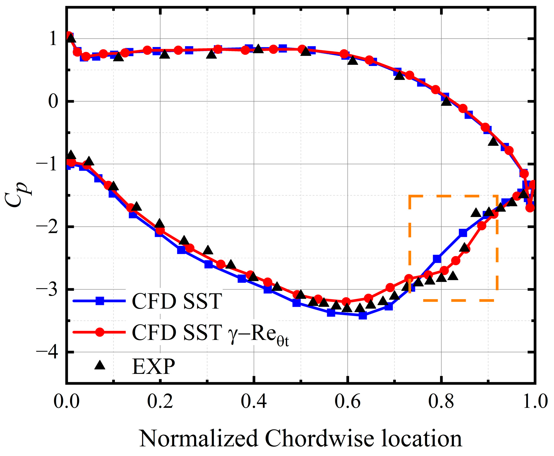
2. Numerical Methods and Validations

The study case in this paper is NASA Stage 67, the most widely used numerical simulation subject. The rotor has 22 blades with 34 stator blades. The relative Ma at the tip reaches 1.38, which is typical of transonic flow. More detailed geometry data and experimental results have been published in [26,27]. This paper aims to investigate the variation in compressor performance triggered by the Re under uniform inflow; therefore, the 1-passage computational domain is set up and illustrated in Figure 1. The main parameters at the design point are listed in Table 1.
The computational grid is the O4H-type grid generated with AutoGird5. Meanwhile, the first grid height is limited to 10−3 mm to keep the boundary layer y + <1. To validate mesh independence, three sets of meshes were used. The information is listed in Table 2. The results are shown in Figure 2. Considering the balance of computational speed and accuracy, the medium mesh was finally selected for the subsequent study. After grid-independence verification, the total number of grids for a single passage is 0.74 million. The mesh node distribution of the rotor passage domain is 138 × 75 × 78 in the streamwise, pitchwise, and spanwise directions, respectively.
The RANS and URANS solutions were performed using the k-ω SST turbulence model in ANSYS CFX v18.2 solver. For RANS cases, the second-order high-resolution advection scheme and the auto fluid timescale control are selected to guarantee solution accuracy and convergence speed. All residuals are less than 10−4. The inlet turbulence intensity is set to 5%. The calculation results are displayed in Figure 3 together with the experimental data. It is evident that the pressure ratio performance curves match well with the data from experiments at different rotational speeds, and the largest error occurs at the stall point at 1.0n, which is 1.7%. Although the deviation in the efficiency performance curves is larger, the curves are still within the 3% error band, and the results are quite similar to other published ones [28]. Generally, the predicted performance curves display a good match with the published data.
In addition, Figure 4 compares the radial distribution of the total parameters of the rotor alone. It can be found that the calculated results deviate slightly from the experimental data near the hub and shroud. The maximum deviation is less than 1.7% for both parameters, but the overall trends agree well. The above demonstrations prove that the method has the ability to accurately predict compressor performance and flow field details.
Furthermore, to more accurately calculate the flow field at a low Re, the γ R e θ , t ¯ transition model is selected for steady and unsteady calculations. Due to the lack of publicly available compressor test data and geometry in low-Re conditions, the PakB [29] cascade with typical transition flow has been chosen in research [30] to validate low-Re calculations. As shown in Figure 5, the validation case is set up with single blade passage, and the boundary conditions are given according to the experimental data.
Figure 6 illustrates the effect of the γ R e θ , t ¯ transition model in low-Re flows. The results show that both CFD calculation models yield highly coincident C p curves on the pressure side and the fore half of the suction one, but only the γ R e θ , t ¯ transition model can predict the separation and reattachment on the suction side in the 0.7 to 0.9 chordwise range (as shown in the box). This case confirms the accuracy of the γ R e θ , t ¯ transition model in the calculation of low-Re conditions. Overall, the numerical method adopted in this work can predict the performance in various Re conditions. The γ R e θ , t ¯ transition model is adopted in all subsequent low-Re cases.

3. Flow Characteristics of the Transonic Compressor at a Low Re

Firstly, compressor performance maps have been calculated for different Re conditions. The effects of Re on the performance deterioration are evident when the RNI (Reynolds Number Index) is no more than 0.3; therefore, the focus is placed on the conditions with an RNI ≤ 0.3. According to the common lift limits of military aircraft, the effects of Re at altitudes of less than 20 km have been investigated, corresponding to the RNI of about 0.1. The compressor performance curves for different RNI conditions are given in Figure 7, and it can be noted that the performance deterioration increases with the reduction in RNI, and the stall boundary moves toward a small mass flow rate. The Reynolds number corresponding to an RNI = 1 is 1.1 × 10⁶. To study the flow field at a low RNI in detail, URANS calculations have been conducted, in which the timestep is set to 5.6667 × 10⁻⁶ s and a total number of 6600 steps for one rotation. The star marks in Figure 6 are the results of URANS for the PE (Peak Efficiency) points in different RNI conditions. The following flow analysis is mainly carried out on the URANS results at the PE points in each RNI condition. For the transonic compressor, according to the inflow velocity, it is divided into two flow regions of subsonic and transonic with the 0.3 span as the boundary, and the flow characteristics at a low Re are analyzed, respectively.

3.1. Subsonic Flow Regions

In the subsonic flow regions, where the flow structure is relatively simple, the airflow in the blade passage mainly undergoes the turning of the flow direction and the reduction in flow velocity. For a transonic compressor, the flow in the small-radius region near the hub is subsonic.
In the regular condition, the inertia force is strong, the fluid possessing great kinetic energy is not prone to separation, and in low-RNI cases, the viscous force makes the fluid difficult to resist separation. For the compressor, the strong viscous forces at a low Re and the effects of the adverse pressure gradient result in a thickened boundary layer on the solid wall, a buildup of low-energy fluids at the wall, and flow separation. Figure 8 compares the Ma distribution of the 0.2-span section at different Re, as a way to represent the characteristics of the boundary-layer development in the subsonic flow region. The results indicate that with the decrease in RNI, the boundary layer has a significant thickening trend, especially in the fore part of the suction side. For cases of RNIs of 0.3, 0.2, and 0.1, the thicknesses in the low-velocity flow region normal to the blade at the 0.3 chordwise position increased by 1.38, 1.54, and 1.57 times, respectively.
In general, the boundary layer on the pressure surface is relative thin, and most boundary-layer parameters on both sides behave similarly, as evidenced in Ref [31]. Thus, it can be stated that the boundary layers on both sides contribute equally to the growth of the wake. After passing through the blade throat, the flow region in the streamwise location becomes an expansion channel, the relative velocity decreases, and the boundary-layer thickness does not increase significantly. As shown in Figure 9, the wake widens as the boundary layer thickens at a low Re, but the variation in both the width and angular range are relatively insignificant compared to the change in boundary-layer thickness on the suction side.

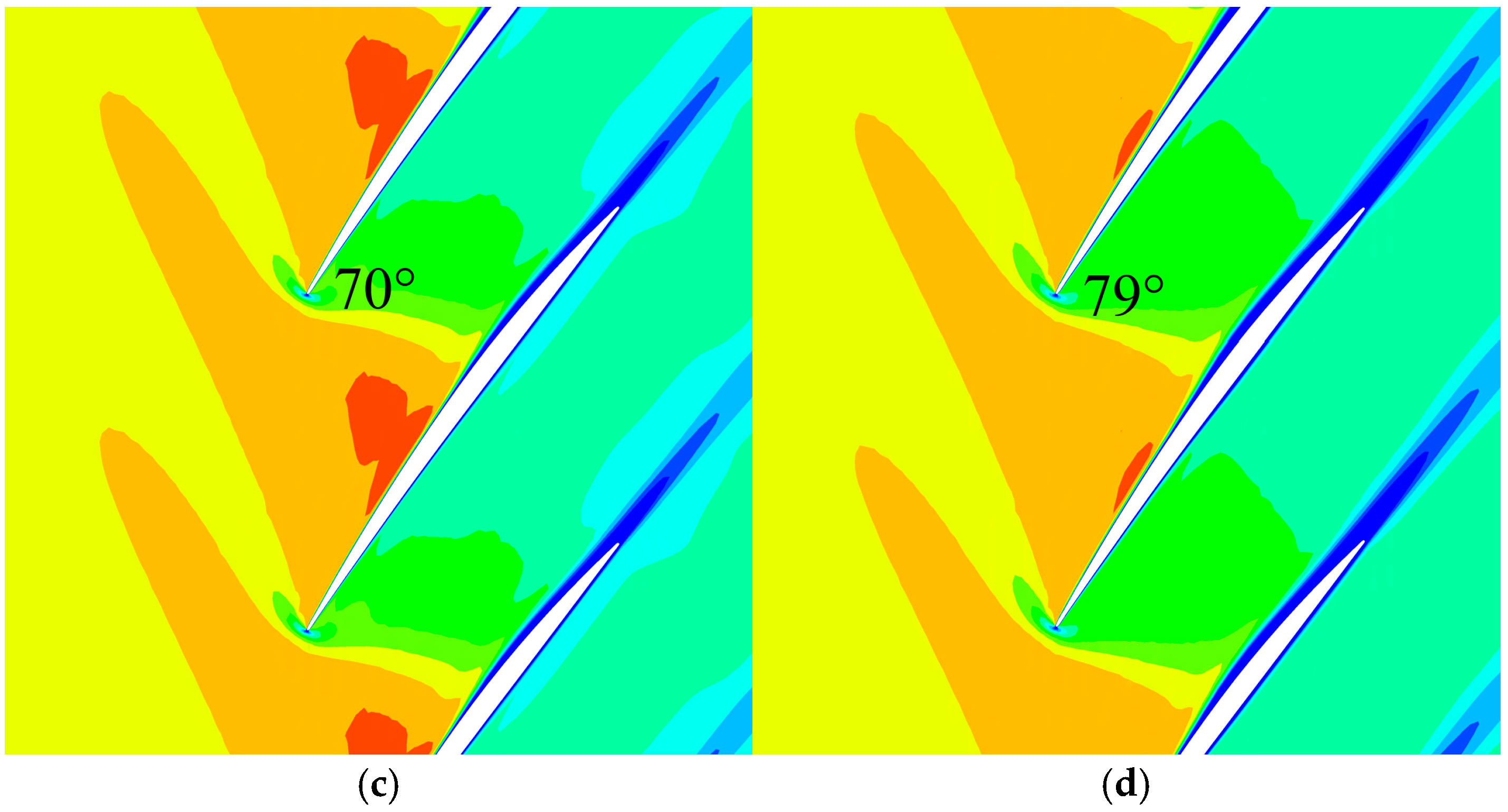
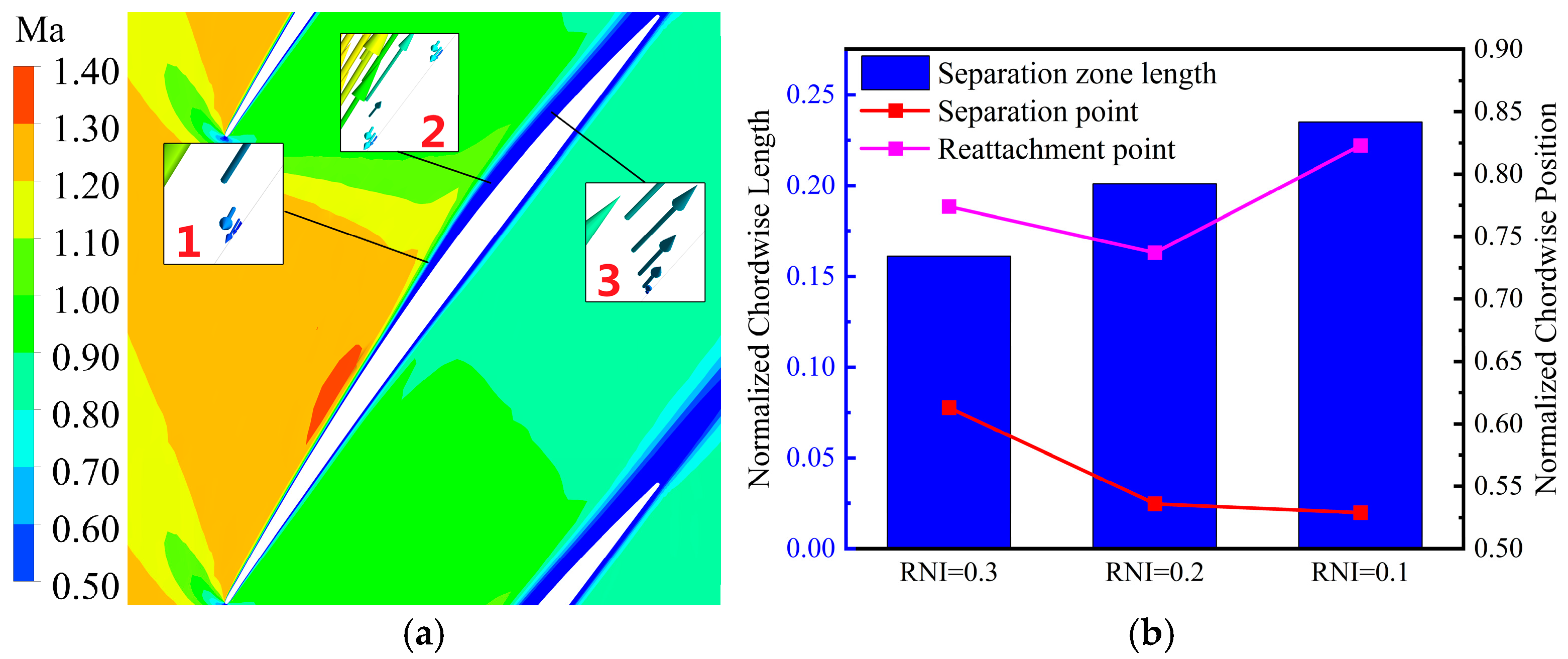
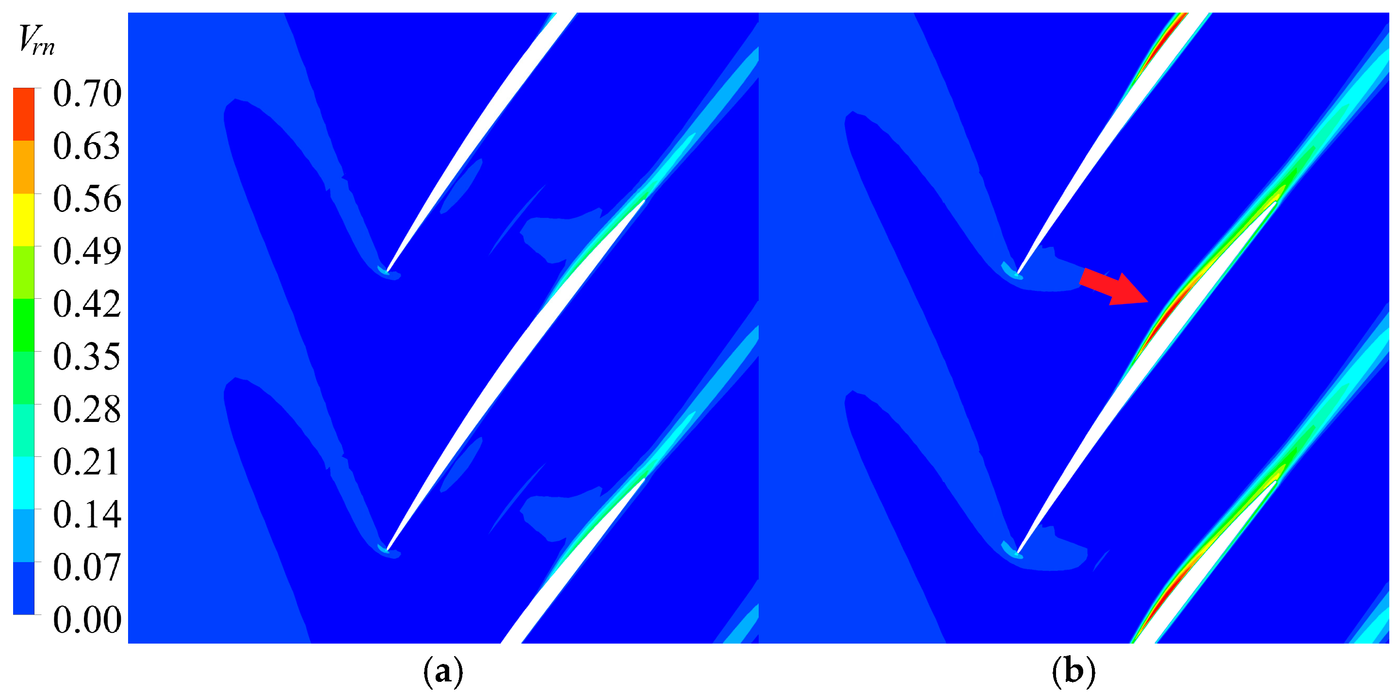
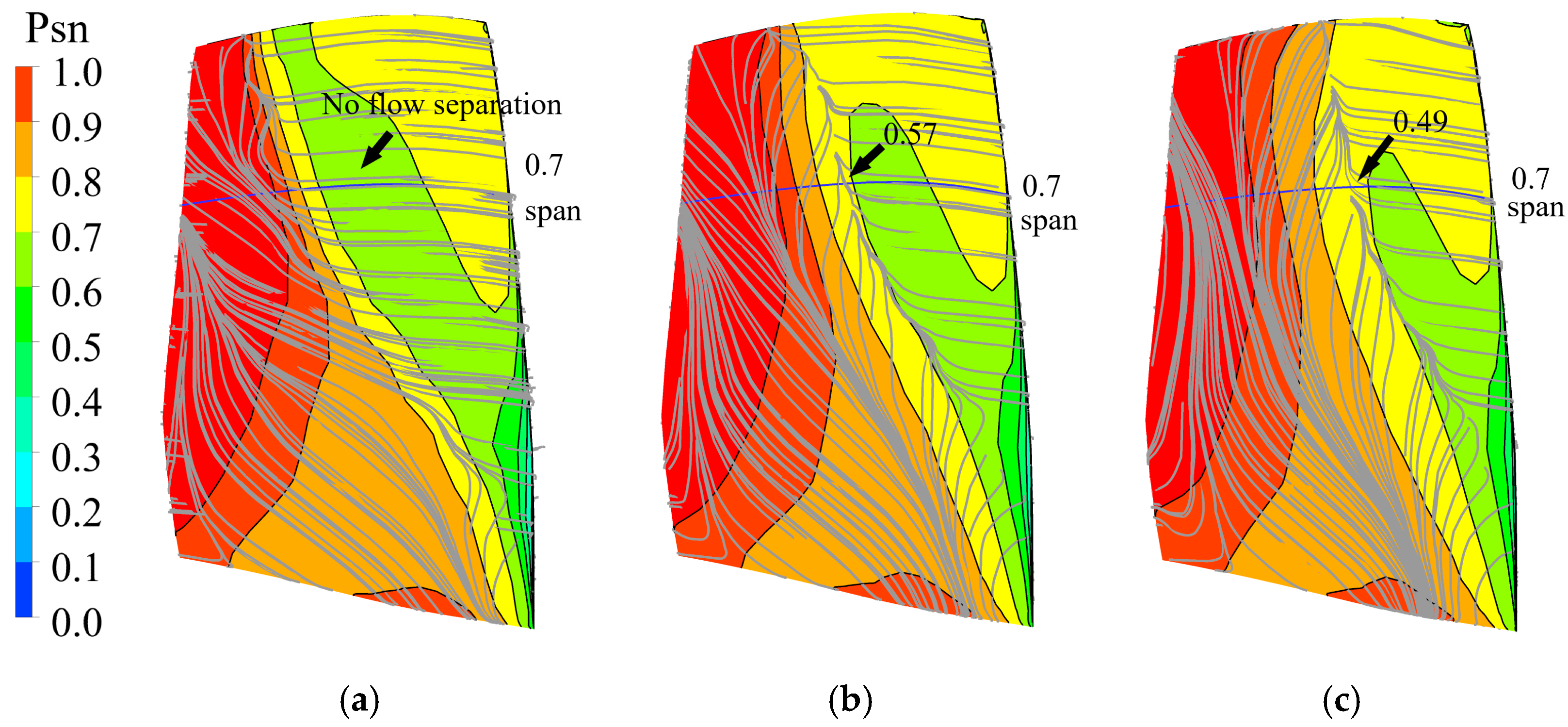
3.2. Transonic Flow Regions

In the transonic flow regions, the flow field differs in several aspects. First, a detached shock wave exists at the leading edge, and the shock angle gradually increases with the decrease in RNI. The inflow Ma at the PE point of each RNI condition is not the same, and the shock structure will be affected by the Ma, but the variation in the shock angle with the RNI is still important. Second, in the fore half of the blade with Ma > 1, the blade boundary layer is thin and changes insignificantly with the RNI. At the position where the shock wave arrives at the adjacent blade, a strong Shock Wave Boundary Layer Interaction (SWBLI) is generated. Low-energy fluids in the boundary layer cannot withstand the large adverse pressure gradient and separate. With increased viscous force action, more pronounced separation of the boundary layer appears, which contributes to the increase in the thickness of the downstream boundary layer. In the blade-to-blade view, the shock angle is the angle between the fitted curve with the relative Ma of 1 and the blade camber line. According to the results shown in Figure 10, as the RNI decreases from 1 to 0.1, the shock angle increases from 60 degrees to 79 degrees at 0.7 span, and it can be clearly observed that the low-velocity region on the blade grows downstream from the shock.
In the RNI = 1 case, the boundary-layer thickness downstream of the shock wave increases without separation. The shock wave in the blade passage enters the boundary layer and extends to the sonic line, and the pressure jump across the shock makes the pressure perturbation propagate upstream in the subsonic region of the boundary layer, increasing the boundary-layer thickness. In the low-RNI cases, significant flow separation of the blade surface fluid occurs after the SWBLI, and reattachment takes place after a certain distance. A schematic of flow separation and reattachment in the 0.7-span section is given in Figure 11a, with point 1 being the onset position of boundary-layer separation and point 3 being the location of reattachment. The separation and attachment points are determined by the appearance and disappearance of the backflow zone on the surface. Point 2 is a location in the separation zone, and it can be seen that there is extensive radial flow in the region where the fluid undergoes separation within the boundary layer. Figure 11b demonstrates the length of the separation zone at the 0.7-span position for different RNI cases. The positions of separation and reattachment change with the Re, which ultimately behaves as an increase in the length of the separation zone.
In the sea level condition, the SWBLI results in the thickening of the boundary layer, but flow separation does not occur, and the flow is almost along the streamwise direction. While in low-Re conditions, the shock induces separation in the boundary layer, and a strong radial secondary flow occurs in the separation region. Figure 12 provides a comparison of the radial-flow velocity distributions in the 0.7-span section for RNI = 1 and RNI = 0.1 conditions. The parameter V r n is the dimensionless radial velocity coefficient, which is the ratio of radial velocity to inlet axial velocity. In the sea level case, the radial flow exists only near the trailing edge, and the radial flow is minor in the region where the boundary layer grows abruptly. The pronounced viscous effects at a low Re lead to severe flow separation within the boundary layer, and extensive radial flow is generated. This indicates that the extensive radial flow at a low Re induces flow separation, resulting in a large increase in the boundary-layer thickness.
Considering that there are essential differences between 3D and 2D flow separation, it is necessary to focus on whether the same characteristics exist for 3D flow separation. Figure 13 compares the limit streamline and Psn (normalized static pressure) distributions on the suction surface, where the normalized static pressure is the ratio of local static pressure to inlet pressure. The blue curve on the surface represents the 0.7-span position, and the gray curves are the limit streamlines. According to Maskell [32], the convergence of the two side-limit streamlines forms the separation line. It intersects with the 0.7 span at 0.57 and 0.49 chordwise positions at RNI = 0.3 and RNI = 0.1 cases, respectively. The curvature of the blade causes the visual distance to deviate from the actual measured value. Compared to the results of RNI = 0.1 in Figure 10, the position of the 3D separation line is advanced by about 0.04 times the chord length, but the overall pattern and flow characteristics are the same and the results are not fundamentally different.

3.3. Challenges for Performance Prediction Due to Low Re Effects

According to the above, the typical flow in the blade passage at a low RNI consists of the following two categories: (1) in the subsonic flow region, the boundary-layer thickness grows significantly in the fore half, and the width of the wake increases slightly; (2) in the transonic flow region, the shock angle of the detached shock wave increases, and the SWBLI leads to a rapid growth in the downstream boundary layer, while the fluid undergoes separation and reattachment, which is accompanied by the wide range of radial flow.
The displacement thickness of the boundary layer at the blade surface constitutes the equivalent aerodynamic profile, which is the most essential feature of the Re affecting the compressor performance and the primary challenge for model prediction. The viscous effects at a low Re cause a significant growth in the boundary layer wrapping the blade, which acts as a film covering the blade. For the inlet airflow, the equivalent blade geometry perceived by the air changes, the blade equivalent thickness increases, and the equivalent flow area of the blade passage shrinks, inducing a series of variations in the flow field. In our previous study [33], it was discovered that the equivalent blade geometry may be the main factor affecting the performance of low-Re compressors. Therefore, the change in the equivalent geometry under the growth of the boundary layer of the blade can be regarded as the source of the performance deterioration at a low RNI.
In subsonic inflow conditions, the change in the equivalent profile does not substantially affect the flow in the blade passage, which mainly influences the width of the wake and increases the loss. The relationship between RNI and wake loss can be obtained from the results of existing studies [34]. In the subsonic flow region, changes in the boundary-layer thickness have a minor effect on the wake, while the variation in the shock structure and radial secondary flow in the transonic flow region are the main factors affecting the compressor performance, which should be considered firstly in conducting modeling calculations. In transonic inflow cases, the change in the equivalent profile will greatly change the shock structure in the blade passage and affect the pressurization process of airflow. Therefore, we will introduce how to assess the equivalent profile in the transonic flow regions next.

4. A Multiline Calculation Strategy Based on the Equivalent Aerodynamic Profile

4.1. Structural Prediction of Detached Shock at Low Reynolds Number

The first step to obtain transonic flow characteristics at a low Re is to accurately predict the detached shock wave. The hyperbolic approximate method proposed by Moeckel [35] provides a simple and rapid determination of the shape and location of the shock. But the assumptions proposed in this method simplify the shock to the single-valued function of the Ma of the inflow, which makes it impossible to predict the shock wave at the leading edge of the blade under the effect of Re.
To accurately obtain the shock wave changes triggered by the equivalent blade geometry, the development of the boundary layer on the curved surface at the leading edge is considered here. An improved model of a detached shock wave at a low Re is developed by taking into account the effect of the equivalent leading-edge geometry on the shock wave. The first thing is to derive the equivalent geometry, since there is no flow mixing near the leading edge; therefore, only the 2D flow effects in the span section on the boundary layer need to be considered, as illustrated in Figure 14. For the 2D flow at a fixed spanwise position, the stagnation point of the inflow is the coordinate origin, the contour line of the blade along the streamwise direction is the x-axis, and the normal direction along the solid wall is the y-axis.
The differential equations for the boundary layer of the curved surface are listed as follows:
V x x + V y y = 0
V x t + V x V x x + V y V y y = 1 ρ p 0 x + 2 V x y 2
V x R = 1 ρ p y
The curvature radius of the blade leading edge R is far greater than the actual displacement thickness of the boundary layer δ * . Therefore, the effect of centrifugal force on p y can be neglected, and the equations for the curvature boundary layer degenerate into the equations for the flat-plate boundary layer, which can be used to calculate the variation in the leading edge δ * at different spans. Figure 15a compares the development of δ * at the leading edge for different RNI conditions. The δ * for the 0.7-span section in Figure 15b is measured at 0.0003 m from the stagnation point. The boundary-layer thickness is normalized with the CFD results for the RNI = 1 case. The results depict that the improved model can accurately predict δ * on the suction and pressure sides at the leading edge with a maximum error of no more than 3.2%.
In the original Moeckel method, the angle η between the sonic line and normal to main flow direction is a fully empirical parameter and a critical parameter for solving the detached shock wave. The empirical formula constructed by Qiu [36] based on the fitting of the CFD results is selected here, which has a good accuracy at inflow Mach numbers less than 3, as shown in Equation (4).
η = M a 0 1.2
In low-RNI conditions, the variation in the equivalent blade contour and the flow angle at the surface sonic line change the deflection angle δ m a x as well. The parameter δ m a x is related to the curvature radius of the sonic point on the solid wall surface, and it illustrates the relationship between δ m a x and the RNI. Figure 16 gives the relationship of δ m a x as a function of the RNI at M a r e l = 1.2 , which is a statistically obtained from CFD calculations for the blade-span sections with an inflow relative Ma of 1.2. The angle δ m a x changes with the inlet conditions; therefore, the value of δ m a x needs to be determined according to the inflow conditions in practical calculations.
On the basis of CFD results, the effects of the variation in δ m a x with the RNI on η are approximately summarized as the relationship shown in Equation (5). In the regular RNI case, δ R e , m a x is equal to δ m a x .
η = δ R e , m a x δ m a x M a 0 1.2
By taking the above equation as the fixed solution condition for the Moeckel method, it is possible to predict the structural changes in shock waves for different RNI cases. Figure 17 compares the results of the improved model for predicting detached shock waves under different cases. In regular RNI conditions, the boundary layer near the leading edge has minor effects on the curvature radius, and an accurate shock wave structure can be predicted in the original Moeckel method. The shock wave on the pressure surface has a shock angle of 57 degrees (angle between the chord line and the shock wave) and intersects with the adjacent blade at 0.72 times the chord length. In low-RNI conditions, the growth of the surface boundary-layer thickness is not negligible, and the effect of the equivalent blade contour on the shock needs to be considered. The original Moeckel method does not include the effects of increased boundary-layer thickness at a low RNI; the results are almost identical to the RNI = 1 case, which causes a large deviation in the prediction for low-RNI cases. The improved model can accurately predict the angle of the detached shock wave, as well as the chordwise position of the intersection of the shock wave with the adjacent blade suction side. The final shock angle of the shock wave on the pressure surface is obtained as 76 degrees at an RNI = 0.1, the intersection with the neighboring blade is 0.59 times the chord length, and the shock angle is significantly increased, which greatly advances the chordwise position of the SWBLI.

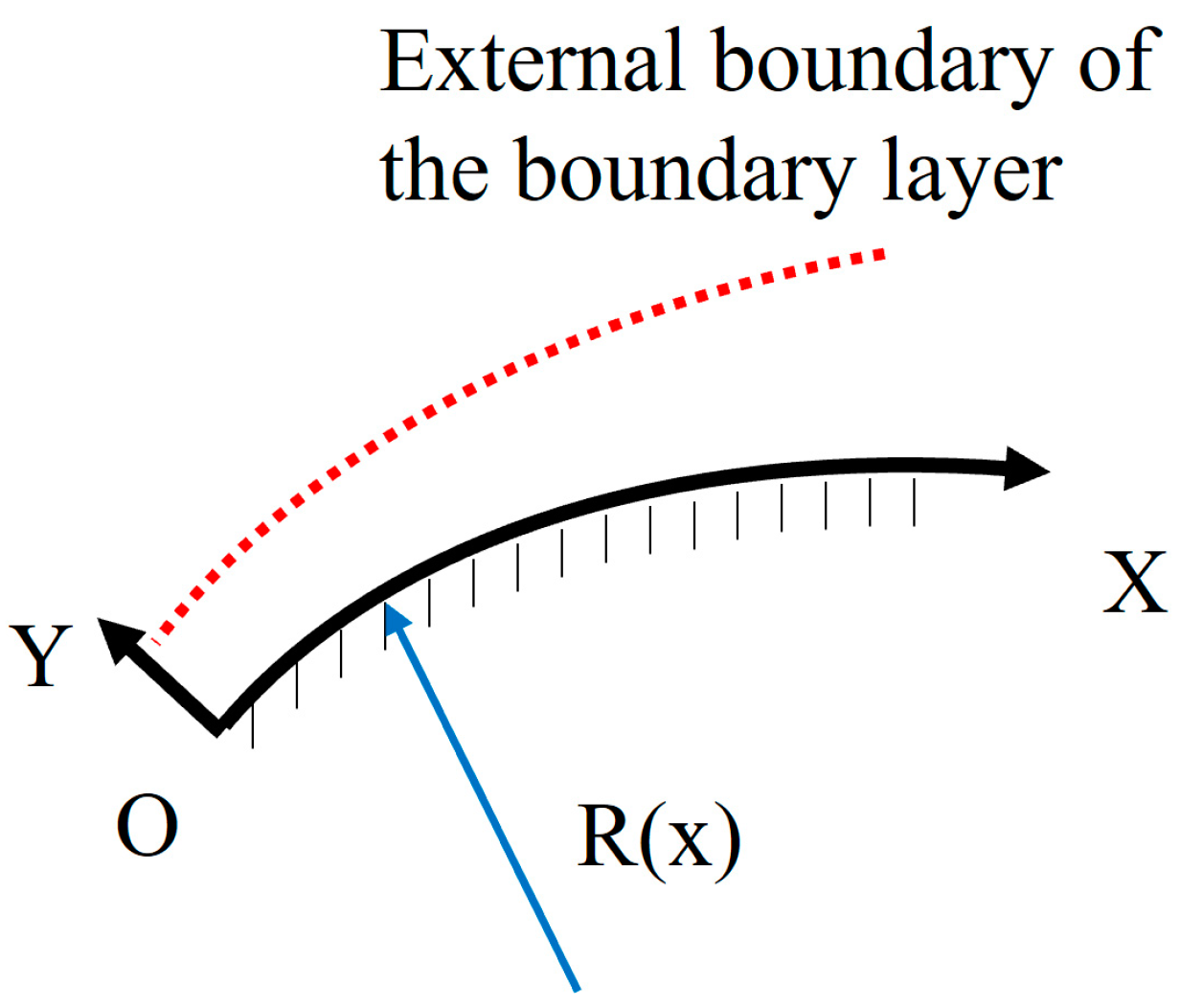
4.2. Equivalent Aerodynamic Profile Prediction Based on Boundary-Layer Theory

The improved Moeckel method presented in Section 4.1 can accurately evaluate the detached shock wave for low-RNI conditions. What is more important is that this method identifies the chordwise position of the intersection point of the shock with the adjacent blade. The intersection point is approximately regarded as the onset of the SWBLI and the starting point of the growth of δ * on the blade surface. According to the results of calculations, the radial flow on the suction surface is enhanced at a low RNI, and the boundary layer on the surface has typical 3D features. However, the 3D boundary-layer equations are complicated and difficult to solve; therefore, this section aims to simplify the boundary layer to a 2D solution on a section with a certain span.
The assumptions used here enable the radial flow characteristics of the 3D boundary layer to be extracted, and, therefore, it can be solved in the simplified 2D problem. The point of modeling 3D flow is to determine the velocity profile of radial flow, also known as cross-flow within the boundary layer. Equation (6) gives the relationship between boundary-layer streamwise and crosswise velocity profiles and wall friction, suggested by Prandtl [37].
u = U y δ * 1 n w = ϵ U y δ * 1 n 1 y δ * 2 = ϵ u 1 y δ * 2
where w represents the velocity component of the cross-flow, which for the blade is the spanwise flow over the surface. The parameter ϵ is the tangent of the angle between the direction of friction stress and the direction of air flow outside the boundary layer, which is generally obtained based on boundary conditions and mathematical methods. According to Ref [38], the agreement with Gruschwize results is better with n = 7 , and combined with the main flow velocity in the blade passage, the cross-flow and streamwise velocity distributions in the boundary layer can be calculated.
The relationship between the increased δ * due to the cross-flow at the blade surface can ultimately be derived based on the approach of Karimipanan [31].
δ * = 0 δ * ρ u w ρ e u e 2 d y 0 δ * ρ w ρ e u e 1 u u e d y
where ρ e and u e represent the density and velocity at the edge of the boundary layer, respectively. To simplify the calculations, the density within the boundary layer is assumed to be constant. Although this assumption seems to affect the accuracy of the calculations, in mildly compressible flow with Ma < 2, neglecting spatial differences in density has little effect on the velocity profile and the development of the boundary layer. Based on the above conditions, it is eventually able to calculate the additional displacement thickness due to the cross-flow. The results of boundary-layer thickness prediction downstream of the SWBLI for different RNI cases are given in Figure 18. Note that the boundary-layer downstream from the shock increases rapidly and then slowly in all conditions, which is because the SWBLI changes the boundary-layer growth mechanism, and the thickness rapidly increases to a certain value before it slowly grows according to the boundary-layer growth curve. The improved model provides an accurate prediction of the onset of interaction effects on the boundary layer, as well as the growth trend in various RNI cases. At the same chordwise position, the improved model has a maximum prediction error of 7.8% for the boundary-layer thickness. Overall, this model provides accurate results for a detached shock wave by considering the Re effects on the equivalent geometry of the blade’s leading edge, and it enables reliable predictions of the equivalent profile in low-Re cases with consideration of the radial flow.

4.3. Partitioned Multiline Calculation Targeted at Equivalent Aerodynamic Profile

The change in equivalent profile will lead to variation in the operating state at different spans, and it ultimately macroscopically manifests as the variation in the radial distribution of the blade load, as shown in Figure 19. The blade load at different spans is normalized with the load of the rotor blade. In the regular condition of RNI = 1, the blade load at the PE point is more evenly distributed at different spans. As the Reynolds number decreases, the distribution of the blade load along the radial direction is redistributed. The distribution pattern of the blade load varies less in the subsonic flow region near the hub, and in the transonic flow region, the blade load increase rapidly at a low Re, exceeding the load in the regular condition.
Due to the redistribution of the radial blade load at a low Re and the strong differences in the flow region at various spanwise positions, a partitioned multiline averaging method is proposed to rapidly calculate the transonic compressor performance under Re effects. This approach can be regarded as using the mean-line method multiple times at different spans. For a single-stage transonic compressor, the row-by-row calculation methodology has been used, and the attack-angle and deviation-angle models at the design point given by NASA [9] are used in this work.
There is no standardized classification of loss in the compressor, and the combination of loss models used by different researchers varies widely. Generally, though, for a transonic compressor, the loss coefficient includes three categories: profile loss ω b l a d e , shock loss ω s h o c k , and secondary flow loss at the tip ω t i p and hub ω h u b . Different combinations of loss models need to be considered for sections at different spans, which can be seen in Figure 20. Based on the analyses of flows and the experience of using loss models, 0.3 and 0.9 spans are selected as the dividing line between regions. In the region of a 0 to 0.3 span, the airflow is subsonic in the blade passage, and the hub loss and profile loss are mainly considered. At a 0.3 span and above, the airflow is transonic, requiring consideration of profile loss and shock loss. As for the region above a 0.9 span, the addition loss due to tip leakage needs to be taken into account. The change in the value of the dividing line is small with the variation in the working conditions as well as the operating points. For example, the difference between the transonic-flow onset positions at the choke and stall points at the design rotational speed does not exceed 0.7%. Therefore, variations in the dividing line are generally not considered when using loss models in sub-regions.
Additionally, the existing loss models and stall criteria are proposed for regular Re conditions, and to broaden their applicability at a low Re, the parameters of the models need to be modified in combination with the equivalent profile. The various types of loss models selected and their physical correlation with the equivalent profile at a low Re are introduced in detail below.
The profile loss is primarily due to the boundary layers of on both sides of the blade converging at the trailing edge and forming the wake. Lieblein et al. [39] have summarized the relationship between load and loss for arbitrary flow conditions from numerous experiments on 2D, low-pressure cascades:
ω b l a d e = 2 θ c c σ c o s β 2 c o s β 1 c o s β 2 2 2 H 3 H 1 1 θ c c σ H c o s β 2 3 1 + i i m i n 2 i s t a l l i m i n 2
θ c in the above equation is the wake momentum thickness, H is the wake form factor, σ represents the blade solidity, and β 1 and β 2 are the air angles at the inlet and exit, respectively. Koch and Smith [34] have utilized compressible boundary-layer theory to expand the loss relation of Equation (8) to a wider range of Ma and Re, and they have considered additional factors such as flow passage contraction. They established a correlation between the dimensionless wake momentum thickness, trailing-edge shape factor, and other relevant variables. It is corrected at off-design points by the empirical relationship with the angle of attack at the minimum loss point. In low-RNI cases, the boundary-layer thickness of both sides of the blade at the trailing edge can be derived from Section 3, and the correlation between θ c c and the RNI based on the physical flow can be obtained from Ref [34]. The profile loss model at a low Re can be corrected by changing the θ c c and H in Equation (8).
The variation in the operating point of the transonic compressor changes the shock structures of the blade passage; therefore, the dual shock model proposed by Bloch [40] is the most applicable. The total pressure relationship across the first detached shock wave in the dual shock loss model is as follows:
p 2 * p 1 * = k + 1 M a 1 2 s i n 2 ψ k 1 M a 1 2 s i n 2 ψ + 2 k k 1 k + 1 2 k M a 1 2 s i n 2 ψ k 1 k k 1
where k is 1.4, representing the specific heat ratio of ideal gas. In the original dual shock loss model, the shock angle ψ is calculated from the classical Moeckel detached shock wave model. As for a low Re, an improved detached shock wave model has been developed, as presented in Section 4. It is feasible to calculate the detached shock loss at a low Re based on the shock angle in the improved model. The point is to bring the shock angle ψ calculated from the improved detached shock wave model into Equation (9).
The secondary flow loss consists of tip loss ω t i p and hub loss ω h u b . In this work, the secondary flow loss is considered using the empirical model by Hearsey [41] and modified by Boyer [42].
ω t i p = ω b l a d e T l o s s 2 r r h u b r t i p r h u b 1 3 1 + i i m i n 2 i s t a l l i m i n 2 r > r m i d ω h u b = ω b l a d e H l o s s 1 2 r r h u b r t i p r h u b 3 1 + i i m i n 2 i s t a l l i m i n 2 r < r m i d
where T l o s s and H l o s s are the correlation coefficients of secondary flow loss at the tip and hub region, respectively, which are obtained by calibrating to the specific research subject. Equation (10) utilizes ω b l a d e to estimate the distribution of secondary flow loss along the spanwise position and takes into account the fact that the tip loss grows with the increasing blade load. By associating ω t i p and ω h u b with the improved profile loss ω b l a d e corresponding to the low-Re conditions, an improved secondary flow loss model related to the inlet Re is developed.
Although the real stall behaviors cannot be reproduced in low-dimensional models, it is possible to establish criteria to identify the stability boundary. Aungier [43] presents a parameter for the equivalent relative velocity ratio W R E , to determine whether or not the compressor reaches the stall boundary.
W R E = p 02 r e l p 2 p 01 r e l p 1 < 0.15 + 0.11 t b / c 0.25 + 10 t b / c 1 + 0.4 θ σ / 2 s i n θ / 2 c o s γ 0.65
where t b , c , θ , σ , and γ stand for the blade maximum thickness, blade chord length, camber angle, solidity, and stagger angle, respectively, which are parameters related to the blade geometry. The calculation of the multiline averaging method will be carried out in the following section, using the loss models and stall criteria described above. At a low RNI, the dimensionless blade maximum thickness t b / c in Equation (11) should be replaced by the maximum thickness of the equivalent blade geometry, considering the displacement boundary-layer thickness δ * , while the thickness can be calculated using the improved model in Section 4.2.

5. Results and Discussion

To produce accurate low-Re performance predictions, the first thing to do is to ensure that the improved method has a good computational accuracy in different spanwise regions. Figure 21 compares the results of span section calculations for regions with different spans using the original loss models and improved ones. In region 1, the difference between the original and the improved method is small due to the fact that the losses are less affected by the Re. In regions 2 and 3, the shock loss in transonic flow is rapidly increased in low-Re cases, which is better captured by the improved method. Taking the efficiency characteristic map for region 2 as an example, the use of the improved models achieves a 2.6% improvement in accuracy compared to the original models.
To display the effect of the improved loss models, Figure 22 depicts the detailed loss coefficient distribution at a 0.95 span over the full angle of attack range at RNI = 0.1 for different loss models. The dashed line and the solid line indicate the results of the original models and the improved loss models. The original loss models fail to take into account the variation in the equivalent blade profile at a low Re, yielding a constant profile loss coefficient and lower tip and shock loss coefficient curve. The loss coefficients calculated by the improved loss models change with the operating point and are slightly higher than those of the original models. In addition, the improved shock loss model can simulate the variation in the detached shock at a low Re and predicts much higher shock loss coefficients than the original one, reaching 0.0308 at the stall point.
After validating the computational results for sections with different spans and the results of the improved loss models, Figure 23 gives a comparison of the performance of the compressor in low-RNI conditions obtained in different approaches. The original method does not consider the change in the equivalent aerodynamic profile due to the boundary layer at a low RNI; therefore, the predicted performance is poorly matched with the CFD results. The improved method, which is based on more accurate physical assumptions, develops more realistic total pressure loss models, and therefore the predicted performance is in better agreement with the CFD results. Compared with the original method, the total pressure prediction error at the stall point is reduced from 1.7% to 0.23% and the mass flow prediction error is reduced by 0.67%. In addition, the maximum prediction error for efficiency is reduced from 3.3% to 1.8%, reaching the accuracy of the original 1D method for the sea level condition.
Further, Figure 24 compares the prediction total pressure ratio performance of the improved and the original methods for different Re conditions. As the RNI decreases, the viscous effect leads to an increasingly significant change in the equivalent profile, with the error of the original model becoming progressively greater. In the improved model, due to the usage of equivalent profile loss models, the error is less than 0.31% in different RNI ranges.
In summary, the multiline calculation strategy opens up the computational dimension of the radial direction and is able to solve the problem of blade load redistribution in the radial direction. With the use of improved loss models which take into account equivalent blade profile corrections, it is possible to predict the overall compressor performance in low-Re conditions. Furthermore, the RANS and URANS cases using 24 partitions take 2.5 h and 13 h, respectively, whereas it takes only 5 min via the multiline calculation strategy.

6. Conclusions

In this paper, the Re effects on the flow characteristics of the compressor have been explored by 3D unsteady simulations, and the influence of viscous effects on the microscopic flow mechanism and macroscopic parameter distributions has been analyzed. A multiline calculation strategy has been proposed to predict the shock wave structure at a low Re based on the variation in the equivalent geometry of the blade’s leading edge, and the 3D flow separation and radial flow induced by the SWBLI have been used to predict the increase in the thickness of the boundary-layer displacements on the surface of the blade. The remarkable findings are as follows:
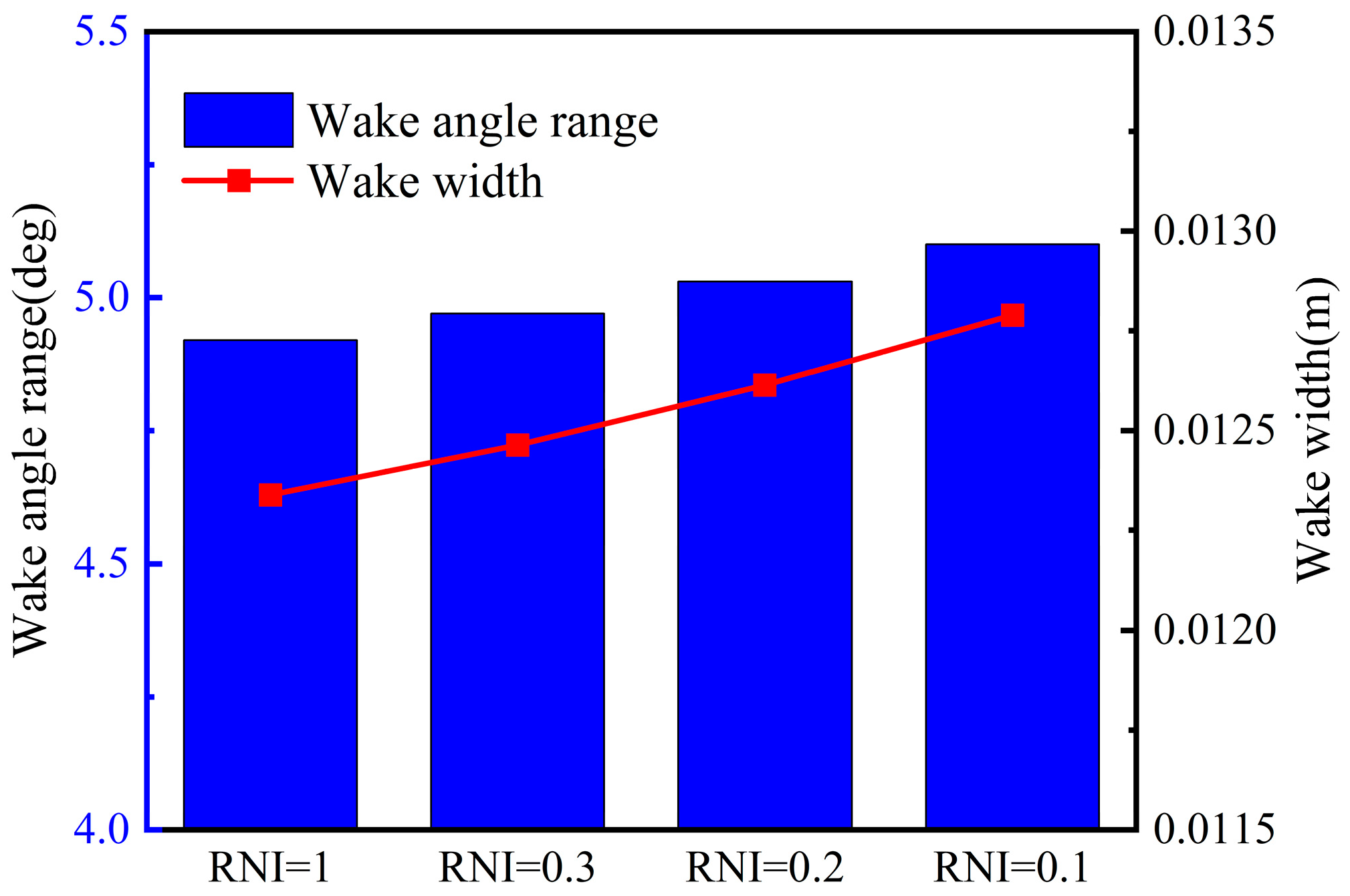
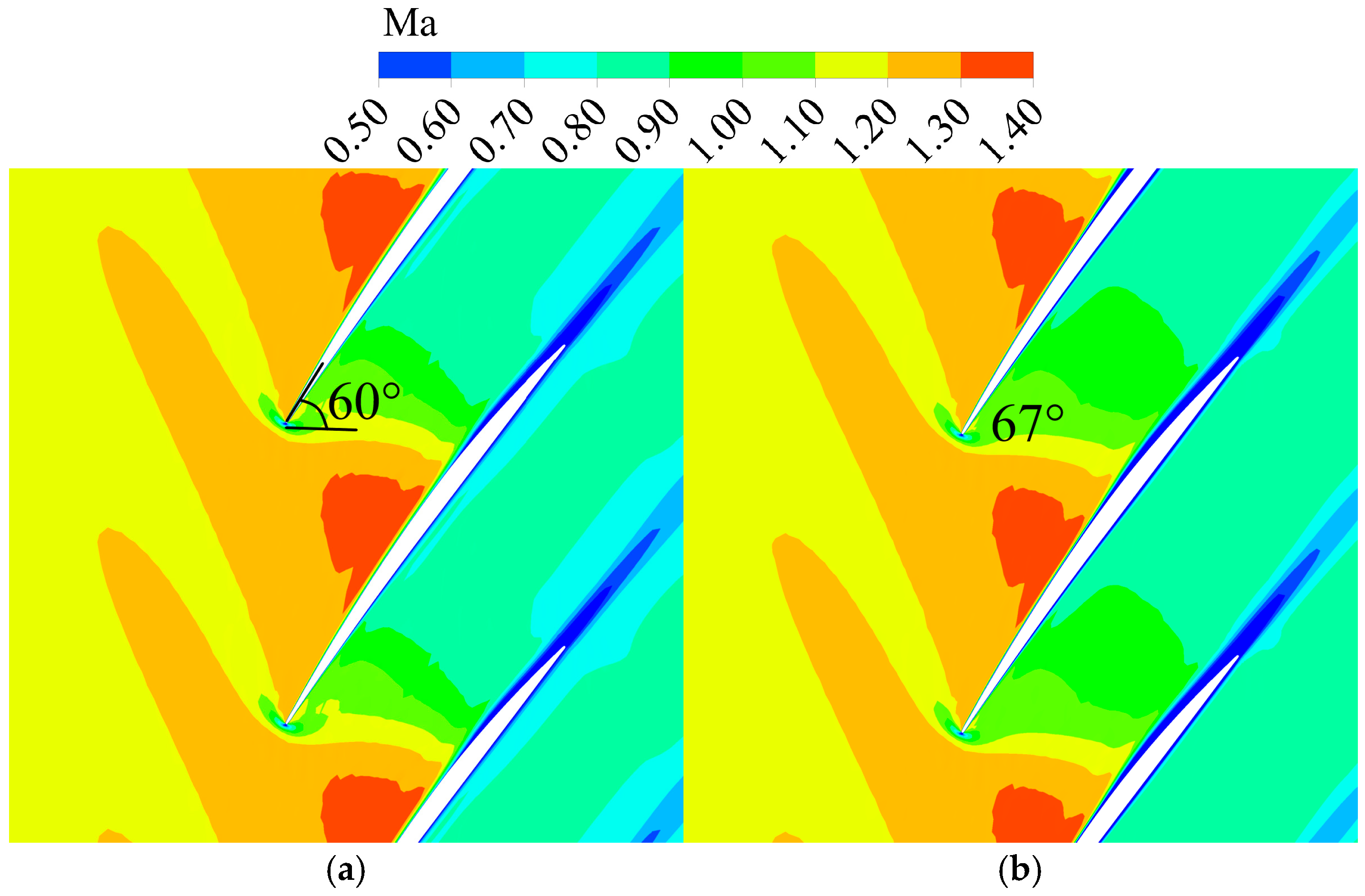
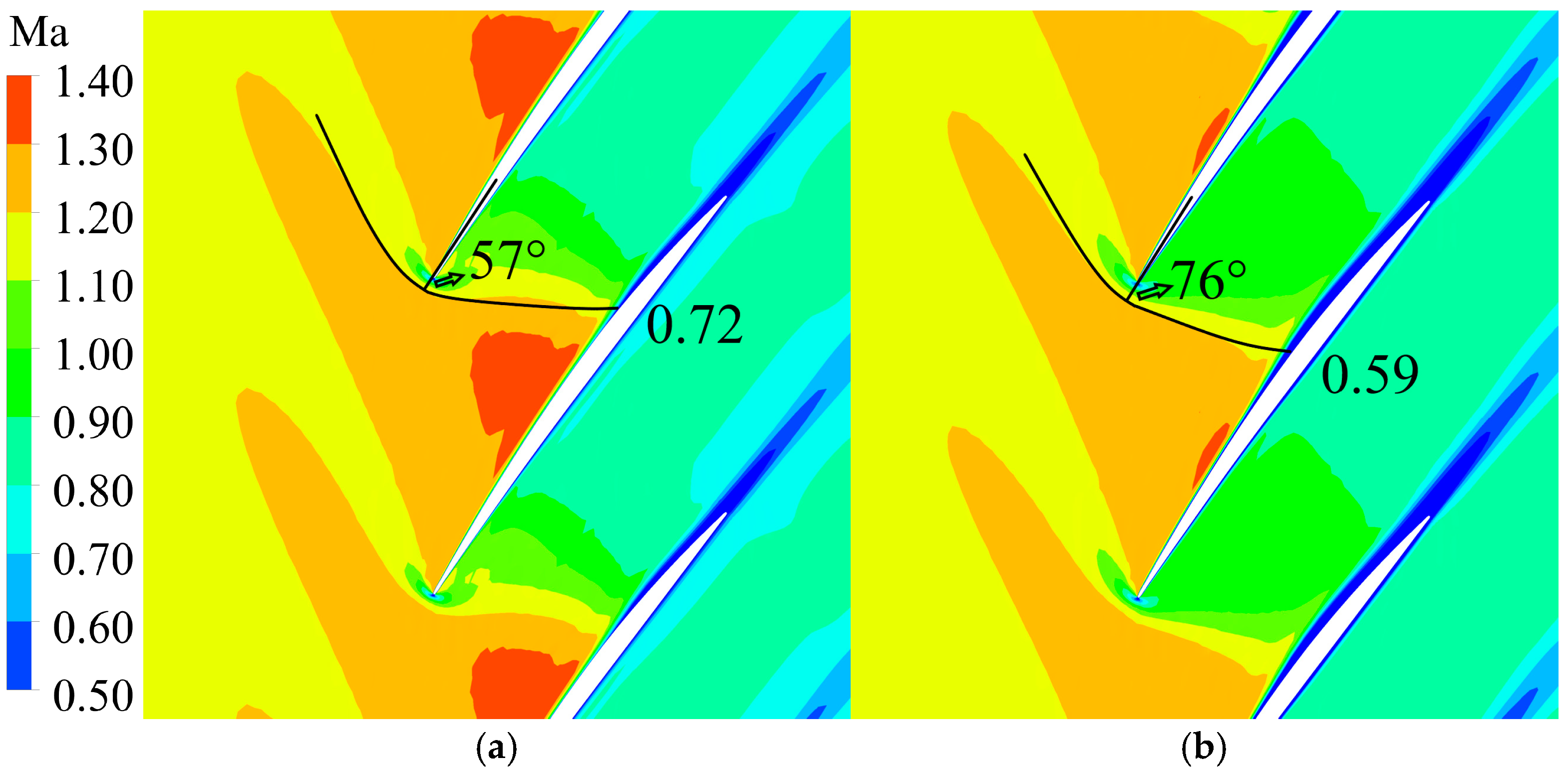
  • The microscopic influence of a low Re on the compressor flow field is mainly reflected in the viscous effect on the boundary layer of the blade surface. In the subsonic region, the development of the boundary layer is accelerated, and the width of the wake increases at a low Re. In the transonic region, the boundary layer interacts strongly with the shock wave at a low Re, and the flow separation enhances the change in the boundary layer. Both of them cause the increase in the boundary-layer thickness, changing the equivalent aerodynamic profile.
  • Based on the boundary-layer theory, a prediction model is proposed for the growth of the boundary layer on the blade in the transonic region. Starting from the development law of the boundary layer at the leading edge of the blade, the maximum prediction error of the boundary-layer thickness at the leading edge is 3.2%. In addition, a detached shock prediction model applicable at a low Re is developed on the basis of the Moeckel method, which is able to accurately predict the shock parameters. The boundary layer calculation method is proposed for the SWBLI, with an equivalent aerodynamic profile calculation error of no more than 7.8% at different Re.
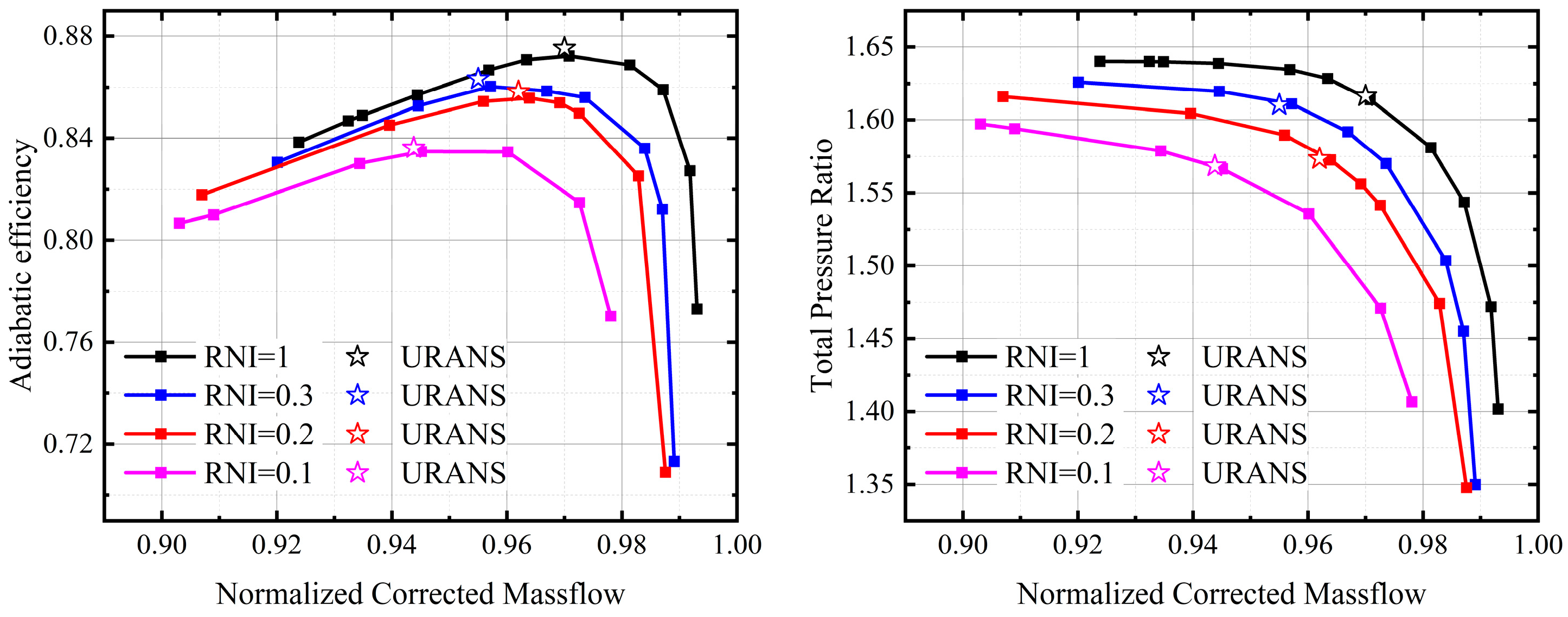
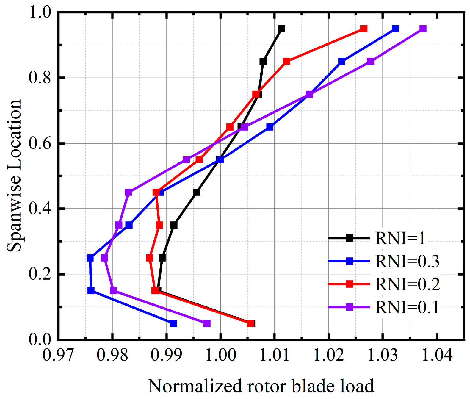
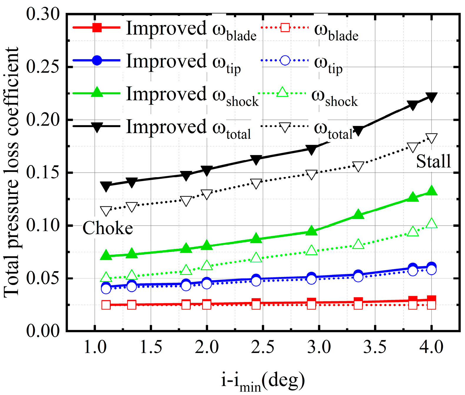
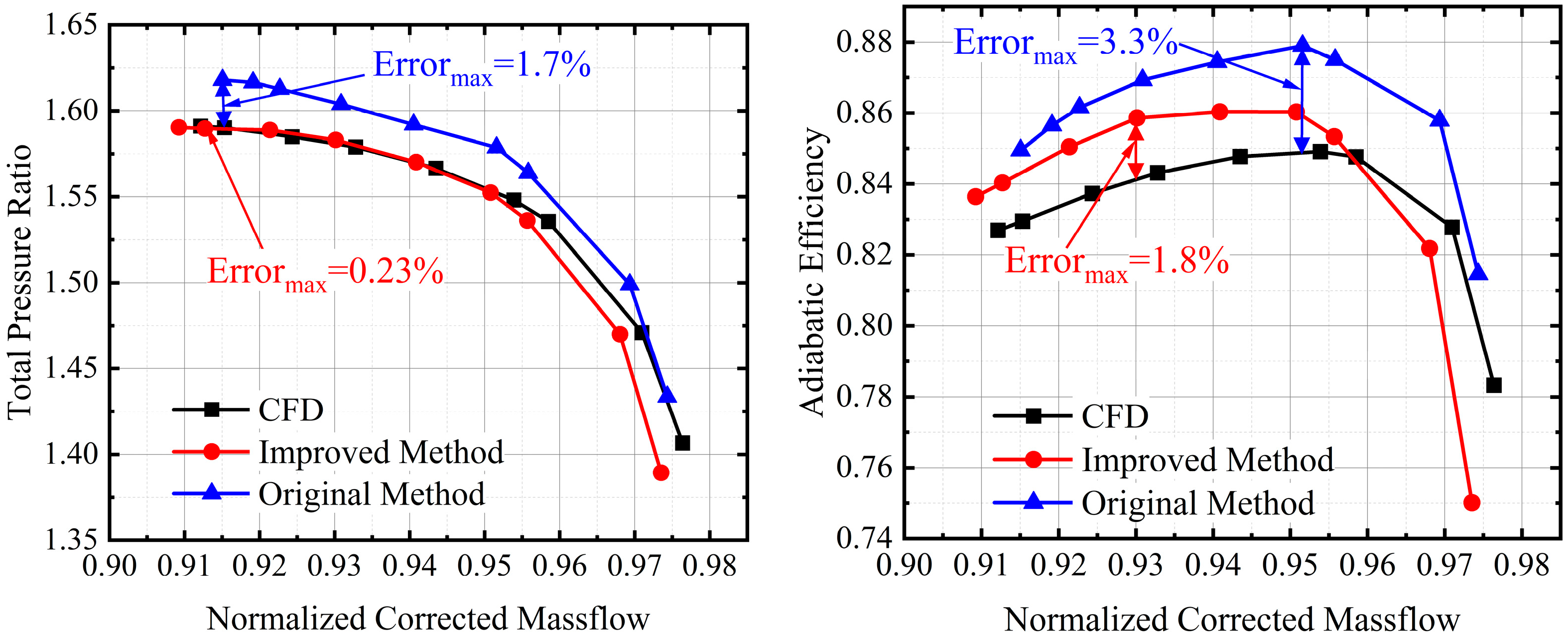
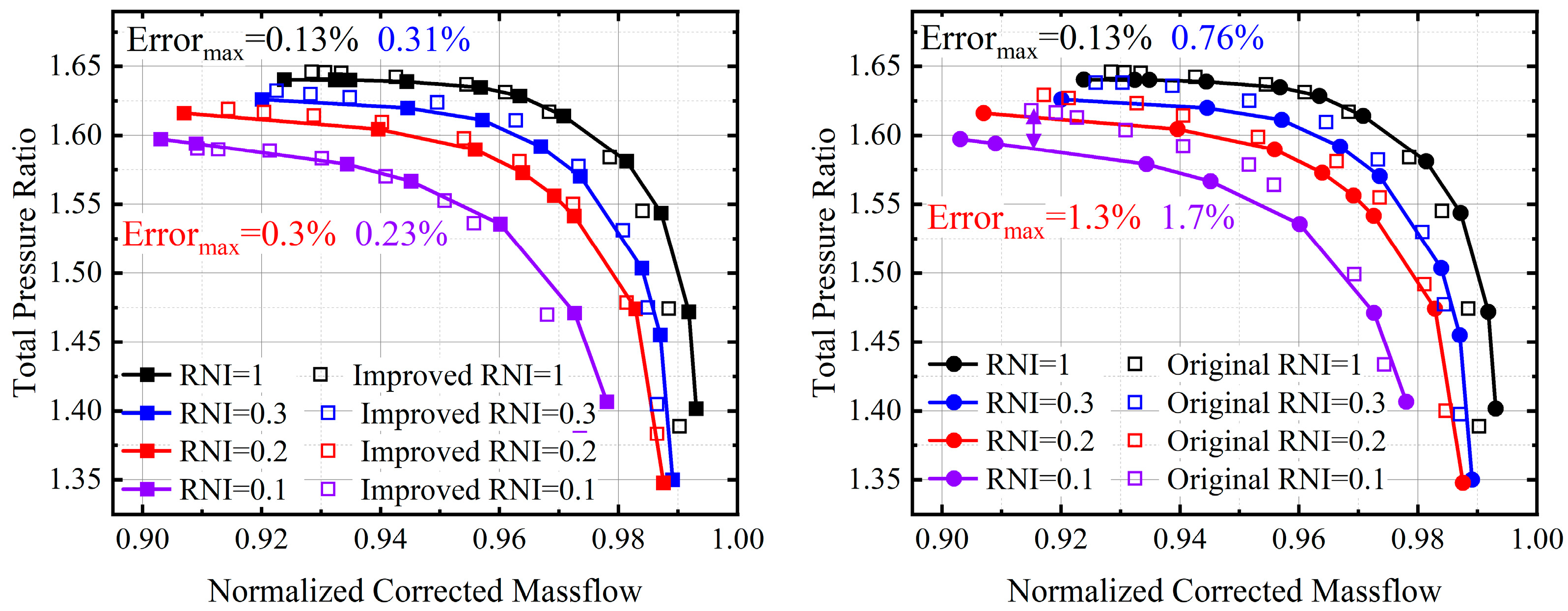
  • A partitioned multiline calculation strategy based on the equivalent profile is proposed. This strategy modifies the effect of the equivalent profile on the loss models and stall criteria, and it accurately calculate the performance at different spans with a maximum error of less than 2%, which marks an improvement of 2.6% in accuracy compared to the original method. The calculation strategy that takes into account the equivalent profile and radial load redistribution opens up the computational dimension in the radial direction, and it improves the accuracy of the overall performance of the compressor at a low Re, with a pressure ratio error of only 0.23% and an efficiency error of 1.8% at an RNI = 0.1. Considering the assumptions made in the calculation process, the method may not be applicable for an Ma > 2. In the lower Re range, new flow phenomena may occur, rendering the method inapplicable.

Author Contributions

Conceptualization, D.S., T.P., X.Z. and Z.L.; methodology, D.S. and X.Z.; software, D.S. and X.Z.; formal analysis, T.P., X.Z. and Z.L.; investigation, D.S. and T.P.; data curation, D.S. and Z.L.; writing—original draft preparation, D.S., X.Z. and T.P.; writing—review and editing, D.S., X.Z. and Z.L.; visualization, D.S., X.Z. and T.P.; supervision, T.P. and Z.L. All authors have read and agreed to the published version of the manuscript.

Funding

This research was funded by the National Natural Science Foundation of China (Nos. 52322603, 52176032) and Beijing Nova Program (No. 20220484074).

Data Availability Statement

The authors confirm that the data supporting the findings of this study are available within the article.

Conflicts of Interest

The authors declare no conflicts of interest.

Nomenclature

C p = p p 0 1 2 ρ v t 2 Static pressure coefficient
R N I = p * 10,1325 288.15 T * μ s e a μ Reynolds Number Index
PEPeak efficiency
H Wake form factor
i Angle of attack (deg)
ρ Density (kg/m3)
p Pressure (Pa)
p * Total pressure (Pa)
T * Total temperature (K)
μ Dynamic viscosity (Pa·s)
ψ Shock angle (deg)
σ Blade solidity
V r n Dimensionless radial velocity coefficient (m/s)
δ m a x Deflection angle (deg)
η Angle between the sonic line and normal to main flow direction (deg)
δ * Boundary-layer displacement thickness
ϵ Tangent of the angle between the direction of friction stress and the direction of flow outside the boundary layer
ω Total pressure loss coefficient
t b Blade maximum thickness (m)
c Blade chord length (m)
θ Camber angle (deg)
γ Stagger angle (deg)
θ c Momentum thickness of the wake

References

  1. Slameršak, A.; Kallis, G.; O’Neill, D.W. Energy requirements and carbon emissions for a low-carbon energy transition. Nat. Commun. 2022, 13, 6932. [Google Scholar] [CrossRef] [PubMed]
  2. Perlaviciute, G.; Steg, L.; Sovacool, B.K. A perspective on the human dimensions of a transition to net-zero energy systems. Energy Clim. Change 2021, 2, 100042. [Google Scholar] [CrossRef]
  3. Wassell, A.B. Reynolds Number Effects in Axial Compressor. J. Eng. Gas Turbines Power 1968, 4, 149–156. [Google Scholar] [CrossRef]
  4. Casey, M.V. The effects of Reynolds number on the efficiency of centrifugal compressor stages. J. Eng. Gas Turbines Power 1985, 107, 541–548. [Google Scholar] [CrossRef]
  5. Casey, M.V.; Robinson, C.J. A unified correction method for Reynolds number, size, and roughness effects on the performance of compressors. Proc. Inst. Mech. Eng. Part A J. Power Energy 2011, 225, 864–876. [Google Scholar] [CrossRef]
  6. Casey, M.V.; Krahenbuhl, D.; Zwyssig, C. The design of ultra-high-speed miniature centrifugal compressors. In Proceedings of the 10th European Conference on Turbomachinery Fluid Dynamics and Thermodynamics ETC, Lappeenranta, Finland, 15–19 April 2013; Volume 10, pp. 1–13. [Google Scholar]
  7. Pelz, P.F.; Stonjek, S.S. The influence of Reynolds number and roughness on the efficiency of axial and centrifugal fans—A physically based scaling method. J. Eng. Gas Turbines Power 2013, 135, 1–8. [Google Scholar] [CrossRef]
  8. Horlock, J.H.; Denton, J.D. A review of some early design practice using computational fluid dynamics and a current perspective. J. Turbomach. Trans. ASME 2005, 127, 5–13. [Google Scholar] [CrossRef]
  9. Johnsen, I.A.; Bullock, R.O. Aerodynamic Design of Axial-Flow Compressors; Chapter 10; NASA: Washington, DC, USA, 1965; p. 297. Available online: https://ntrs.nasa.gov/citations/19650013744 (accessed on 14 April 2025).
  10. Howell, A.R.; Bonham, R.P. Overall and stage characteristics of axial-flow compressors. Proc. Inst. Mech. Eng. 1950, 163, 235–248. [Google Scholar] [CrossRef]
  11. Howell, A.R.; Calvert, W.J. A new stage stacking technique for axial-flow compressor performance prediction. J. Eng. Gas Turbines Power Trans. ASME 1978, 100, 698–703. [Google Scholar] [CrossRef]
  12. Smith, S.L. One-Dimensional Mean Line Code Technique to Calculate Stage-by-Stage Compressor Characteristics. Master’s Thesis, University of Tennessee, Knoxville, TN, USA, 1999. [Google Scholar]
  13. Miller, A.S. Compressor Conceptual Design Optimization. Ph.D. Thesis, Georgia Institute of Technology, Atlanta, GA, USA, 2015. [Google Scholar]
  14. White, N.M.; Tourlidakis, A.; Elder, R.L. Axial compressor performance modelling with a quasi-one-dimensional approach. Proc. Inst. Mech. Eng. Part A J. Power Energy 2002, 216, 181–193. [Google Scholar] [CrossRef]
  15. Dahlquist, A.N. Investigation of Losses Prediction Methods in 1D for Axial Gas Turbine. Master’s Thesis, Lund University, Scania, Sweden, 1990. [Google Scholar]
  16. Back, S.C.; Hobson, G.V.; Song, S.J.; Millsaps, K.T. Effects of Reynolds Number and Surface Roughness Magnitude and Location on Compressor Cascade Performance. J. Turbomach. Trans. ASME 2012, 134, 051013. [Google Scholar] [CrossRef]
  17. Liu, Q.; Ager, W.; Hall, C.; Wheeler, A.P. Low Reynolds Number Effects on the Separation and Wake of a Compressor Blade. J. Turbomach. Trans. ASME 2022, 144, 101008. [Google Scholar] [CrossRef]
  18. Xu, H.F.; Zhao, S.F.; Wang, M.Y.; Sheng, X.Y.; Han, G.; Lu, X.G. Investigation of unsteady flow mechanisms and modal behavior in a compressor cascade. Aerosp. Sci. Technol. 2023, 142, 108596. [Google Scholar] [CrossRef]
  19. Pan, T.; Li, T.; Yan, Z.; Li, Q. Investigation of turbulence-induced disturbances and their evolution to stall onset in a compressor cascade using large eddy simulation. Chin. J. Aeronaut. 2025. [Google Scholar] [CrossRef]
  20. Wang, M.; Yang, C.; Li, Z.; Zhao, S.; Zhang, Y.; Lu, X. Effects of surface roughness on the aerodynamic performance of a high subsonic compressor airfoil at low Reynolds number. Chin. J. Aeronaut. 2021, 34, 71–81. [Google Scholar] [CrossRef]
  21. Li, Z.L.; Wu, Y.F.; Li, L.; Lu, X.G.; Han, G. Numerical Investigation of Low Reynolds Number Effects on Energy Loss Inside Centrifugal Compressor with Different Inlet Conditions. Aerosp. Sci. Technol. 2024, 146, 108923. [Google Scholar] [CrossRef]
  22. Cheng, H.; Lu, X.; Zhao, S.; Huang, S.; Zhu, J. Effect of tip clearance variation in the transonic axial compressor of a miniature gas turbine at different Reynolds numbers. Aerosp. Sci. Technol. 2022, 128, 107793. [Google Scholar] [CrossRef]
  23. Cheng, H.; Li, Z.; Zhou, C.; Lu, X.; Zhao, S.; Han, G. Effect of blade surface cooling on a micro transonic axial compressor performance at low Reynolds number. Appl. Therm. Eng. 2023, 226, 120353. [Google Scholar] [CrossRef]
  24. Diehl, M.; Schreiber, C.; Schiffmann, J. The Role of Reynolds Number Effect and Tip Leakage in Compressor Geometry Scaling at Low Turbulent Reynolds Numbers. ASME. J. Turbomach. 2020, 142, 031003. [Google Scholar] [CrossRef]
  25. Irps, T.; Kanjirakkad, V. Wake–Separation Bubble Interaction Over an Experimentally Simulated Axial Compressor Blade Under Low Reynolds Number Flow. ASME. J. Turbomach. 2025, 147, 081018. [Google Scholar] [CrossRef]
  26. Strazisar, A.J.; Wood, J.R.; Hathaway, M.D.; Suder, K.L. Laser Anemometer Measurements in a Transonic Axial-Flow Fan Rotor; NASA-TP-2879; NASA: Cleveland, OH, USA, 1990. Available online: https://ntrs.nasa.gov/citations/19900001929 (accessed on 14 April 2025).
  27. Ferrar, A.M. Measurement and Uncertainty Analysis of Transonic Fan Response to Total Pressure Inlet Distortion. Ph.D. Thesis, Virginia Polytechnic Institute and State University, Blacksburg, VA, USA, 2015. [Google Scholar]
  28. Spotts, N. Unsteady Reynolds-Averaged Navier-Stokes Simulations of Inlet Flow Distortion in the Fan System of a Gas-Turbine Aero-Engine. Master’s Thesis, Colorado State University, Fort Collins, CO, USA, 2015. [Google Scholar]
  29. Murawski, C.G.; Sondergaard, R.; Rivir, R.B.; Vafai, K.; Simon, T.W.; Volino, R.J. Experimental Study of the Unsteady Aerodynamics in a Linear Cascade with Low Reynolds Number Low Pressure Turbine Blades. In Proceedings of the ASME 1997 International Gas Turbine and Aeroengine Congress and Exhibition, Orlando, FL, USA, 2–5 June 1997. [Google Scholar]
  30. Zhang, P.; Lu, J.; Wang, Z.; Song, L.; Feng, Z. Adjoint-Based Optimization Method with Linearized SST Turbulence Model and a Frozen Gamma-Theta Transition Model Approach for Turbomachinery Design. In Proceedings of the ASME Turbo Expo 2015: Turbine Technical Conference and Exposition, Montreal, QC, Canada, 15–19 June 2015; Volume 2B, pp. 1–15. [Google Scholar]
  31. Karimipanah, M.T.; Olsson, E. Calculation of three-dimensional boundary layer on rotor blades using integral methods. In Proceedings of the ASME 1992 International Gas Turbine and Aeroengine Congress and Exposition, Cologne, Germany, 1–4 June 1992; Volume 1, pp. 1–14. [Google Scholar] [CrossRef]
  32. Maskell, E.C. Flow Separation in Three Dimensions; Ministry of Supply, Royal Aircraft Establishment, RAE: Farnborough, UK, 1955. [Google Scholar]
  33. Li, Z.; Zhu, X.; Yan, Z.; Pan, T. Effects of Re on blade load temporal-spatial distribution and correlation with flow stability of transonic compressor under inlet distortion. Aerosp. Sci. Technol. 2024, 147, 109007. [Google Scholar] [CrossRef]
  34. Koch, C.C.; Smith, L.H. Loss sources and magnitudes in axial-flow compressors. J. Eng. Gas Turbines Power Trans. ASME 1976, 98, 411–424. [Google Scholar] [CrossRef]
  35. Moeckel, W.E. Approximate Method for Prediction Form and Location of Detached Shock Waves Ahead of Plane or Axially Symmetric Bodies; NACA TN-1921; NASA: Cleveland, OH, USA, 1949. Available online: https://ntrs.nasa.gov/api/citations/19930082597 (accessed on 14 April 2025).
  36. Qiu, M.; Zhou, Z.G.; Liu, L.L. Prediction of detached shockwaves from leading edge of supersonic cascade. J. Aerosp. Power 2014, 29, 363–373. [Google Scholar]
  37. Prandtl, L. On boundary layer layers in three dimensional flow. 1946, Reps. And Trans. No.64, British M. A. P.
  38. Gruschwitz, E. Turbulente Reibungsschichten mit Sekundärströmung. Ing. Arch. 1935, 6, 355–365. [Google Scholar] [CrossRef]
  39. Lieblein, S.; Roudebush, W.H. Theoretical Loss Relations for Low-Speed Two-Dimensional-Cascade Flow; NACA TN3662; NASA: Cleveland, OH, USA, 1956. Available online: https://ntrs.nasa.gov/citations/19930084888 (accessed on 14 April 2025).
  40. Bloch, G.S. Flow Losses in Supersonic Compressor Cascades. Ph.D. Thesis, Mechanical Engineering Dept, Virginia Polytechnic Institute and State University, Blacksburg, VA, USA, 1996. [Google Scholar]
  41. Hearsey, R.M. Program HT0300 NASA 1994 version. 1994, Doc. No. D6-81569TN, Volumes 1 and 2, the Boeing Company.
  42. Boyer, K.M. An Improved Streamline Curvature Approach for Off-Design Analysis of Transonic Compression System. Ph.D. Thesis, Virginia Polytechnic Institute and State University, Blacksburg, VA, USA, 2001. [Google Scholar]
  43. Aungier, R.H.; Farokhi, S. Axial-Flow Compressors: A Strategy for Aerodynamic Design and Analysis; ASME Press: New York, NY, USA, 2003. [Google Scholar]
Figure 1. Schematic of 1-passage computational domain of the compressor.
Aerospace 12 00349 g001
Figure 2. Comparison of calculation results for different meshes.
Aerospace 12 00349 g002
Figure 3. Validation of compressor performance maps by numerical simulation.
Aerospace 12 00349 g003
Figure 4. Validation of radial parameter distribution at the outlet of the compressor rotor.
Aerospace 12 00349 g004
Figure 5. Schematic of single blade passage computational domain of PakB cascade.
Aerospace 12 00349 g005
Figure 6. Validation of γ R e θ , t ¯ transition model for low-Re flow on PakB cascade.
Aerospace 12 00349 g006
Figure 7. Compressor performance maps for different RNI conditions.
Aerospace 12 00349 g007
Figure 8. Relative Mach number distribution of 0.2-span section in different RNI cases. (a) RNI = 1; (b) RNI = 0.3; (c) RNI = 0.2; (d) RNI = 0.1.
Aerospace 12 00349 g008
Figure 9. Measurements of rotor blade wake at the trailing edge of 0.2-span section.
Aerospace 12 00349 g009
Figure 10. Relative Mach number distribution of 0.7-span section in different RNI cases. (a) RNI = 1; (b) RNI = 0.3; (c) RNI = 0.2; (d) RNI = 0.1.
Aerospace 12 00349 g010aAerospace 12 00349 g010b
Figure 11. Boundary-layer separation and reattachment at the suction surface of a 0.7-span section. (a) Flow schematic for RNI = 0.1; (b) comparison of separation zone lengths.
Aerospace 12 00349 g011
Figure 12. Radial velocity contour at 0.7-span section for two RNI cases. (a) RNI = 1; (b) RNI = 0.1.
Aerospace 12 00349 g012
Figure 13. Comparison of limit streamline and pressure distributions on rotor suction surface with different cases. (a) RNI = 1; (b) RNI = 0.3; (c) RNI = 0.1.
Aerospace 12 00349 g013
Figure 14. Schematic of curvature boundary layer.
Aerospace 12 00349 g014
Figure 15. Improved model and CFD comparison of boundary-layer thickness at rotor leading edge. (a) Boundary layer at 0.7-span section; (b) prediction of boundary-layer thickness.
Aerospace 12 00349 g015
Figure 16. Statistically obtained δ m a x versus RNI at M a r e l = 1.2 from CFD results.
Aerospace 12 00349 g016
Figure 17. Comparison of the predicted results of the improved detached shock wave model for two different RNI conditions. (a) RNI = 1; (b) RNI = 0.1.
Aerospace 12 00349 g017
Figure 18. Improved model prediction results of the onset of the SWBLI and the thickness of the boundary layer for different Re cases at PE point.
Aerospace 12 00349 g018
Figure 19. Comparison of radial distribution of normalized blade load at different Re.
Aerospace 12 00349 g019
Figure 20. Loss model combination approach partition in the spanwise location.
Aerospace 12 00349 g020
Figure 21. Span section performance located in different flow regions at RNI = 0.1. (a) 0.15 span in region 1; (b) 0.55 span in region 2; (c) 0.95 span in region 3.
Aerospace 12 00349 g021
Figure 22. Comparison of results from different loss models at 0.95 span for the case of RNI = 0.1.
Aerospace 12 00349 g022
Figure 23. Comparison of the improved method and original method for predicting results in low-Re condition (RNI = 0.1).
Aerospace 12 00349 g023
Figure 24. Comparison of the improved method and original method for predicting performance in different Re conditions.
Aerospace 12 00349 g024
Table 1. Main parameters of the NASA R67 stage at design point.
ParametersRotorStator
Blade number2234
Rotational speed (rpm)16,042.8/
Mass flow rate (kg/s)33.25/
Total pressure ratio1.63/
Tip clearance (mm)1.006/
Blade tip aerodynamic chord (cm)9.5225.768
Rotor aspect ratio1.56/
Inlet/Exit hub/tip radius ratio0.375/0.4780.5/0.53
Tip relative Mach number1.38/
Table 2. Numbers of different meshes.
Mesh NumberIn BlockRotorStatorTotal
Coarse1.8 × 1041.6 × 1051.1 × 1053.1 × 105
Medium4.2 × 1044 × 1053 × 1057.4 × 105
Fine5.4 × 1045.3 × 1054 × 1059.8 × 105
Disclaimer/Publisher’s Note: The statements, opinions and data contained in all publications are solely those of the individual author(s) and contributor(s) and not of MDPI and/or the editor(s). MDPI and/or the editor(s) disclaim responsibility for any injury to people or property resulting from any ideas, methods, instructions or products referred to in the content.

