A New Aerodynamic Domain Model (ADM) for Enhancing the Reliability of Spin Flight Vehicle Simulations

Abstract

A spin flight vehicle is characterized by its inherent active or passive spinning motion, resulting in complex movements that pose challenges for accurately calculating aerodynamic forces. This often leads to significant discrepancies between simulation results and actual performance. To address the low reliability of simulations for single-wing spin flight vehicles caused by difficulties in aerodynamic force estimation, this paper introduces the concept of an aerodynamic domain model. Based on the configuration of a specific single-wing spin flight vehicle, the model applies rigid body dynamics and uses blade element-momentum theory for aerodynamic calculations. By considering both relative and absolute error characteristics between actual and computed aerodynamic values, the aerodynamic domain model is established with explicit methods for determining error factor function bounds. The theoretical and practical value of the model is demonstrated through a simulation example, showing its ability to represent the range of true aerodynamic forces and moments experienced by the vehicle. This approach reduces the dependence on highly accurate aerodynamic calculations while maintaining engineering feasibility, enabling effective flight risk assessments within a specified range.

1. Introduction

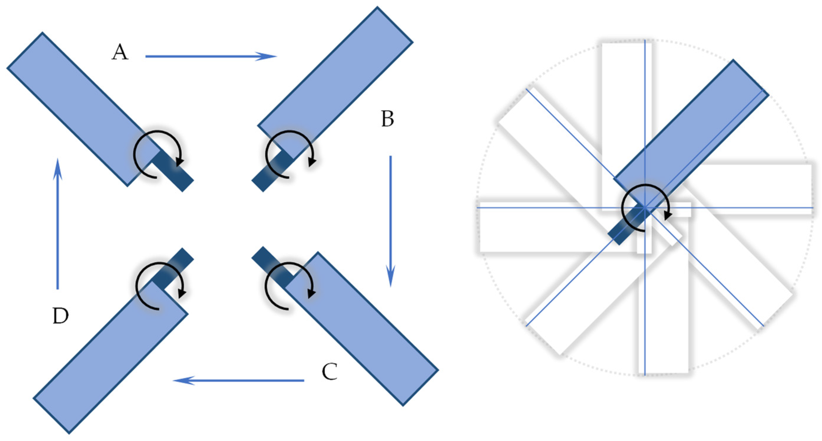
A spin vehicle is an aircraft whose attitude exhibits significant periodic rotational motion during flight, either actively or passively. Figure 1 visually illustrates a typical passive spin vehicle. On the left side, the figure shows how the vehicle’s attitude transitions through four states—A, B, C, and D—due to its spinning motion. On the right side, it depicts the spinning effect relative to the vehicle’s center of mass.

The defining characteristic of a spin vehicle is its pronounced self-rotation, distinguishing it from most conventional aircraft such as fixed-wing, rotary-wing, flapping-wing aircraft, and airships, which generally exhibit non-rotational or non-periodic rotational behavior under normal conditions. This unique motion capability enables spin vehicles to perform tasks that traditional aircraft may find difficult or impossible. In recent years, growing interest and extensive research have been directed toward spin vehicles.

Research on spin vehicles has explored their diverse applications. For example, Kim B. H. et al. applied powerless spin vehicles for deployment in natural and urban environments [1]. Zhang W. et al. designed a single-propeller-controlled spin vehicle that operates independently of passive aerodynamic effects [2]. Suhadi B. L. et al. developed a multi-modal spin vehicle capable of transitioning between ground-to-air flight modes [3]. Win S. K. H. et al. introduced a foldable wing for single-wing spin vehicles [4] and explored their air deployment in disaster-stricken areas [5]. Bhardwaj H. et al. applied foldable wings to both single- and dual-wing spin vehicles, reducing overall footprint by 39% and 69%, respectively [6]. They also proposed a new multi-mode single-wing aircraft capable of operating in both single- and dual-wing flight modes [7]. Sufiyan D. et al. expanded this to three convertible flight modes [8]. Cai X. et al. designed a modular spin vehicle that allows easy reconfiguration using customized wings and control modules [9]. For foldability, Liu W. adapted a fruit wing prototype into a four-fold crease origami wing design [10]. Tong S. et al. created a composite spin vehicle with modules that can be assembled into configurations of 2, 3, or 6 units for quick ground assembly and controlled aerial separation [11].

Research has also focused on the motion characteristics of spin vehicles. Their aerodynamic models often derive from helicopter blade models using methods such as momentum theory, vortex analysis, blade element theory, and slipstream theory [12,13]. For single-wing spin vehicles, Fan Z. applied blade element-momentum theory to single-blade rotors [14]. Matić G. et al. developed a simplified nonlinear dynamic model to describe the fundamental characteristics of spin vehicles in different flight states [15]. Kang S. et al. introduced a discrete method for aerodynamic simulation, avoiding singularities from traditional linearization methods [16]. Tong S. et al. simplified longitudinal motion equations by using a “half-body” co-ordinate system [17]. Win S. K. H. improved flight dynamics by optimizing wing shape and flap angle of attack, finding that a gradually widening wing enhances the spin state [18]. Jung B. K. and Rezgui D. applied the Polhamus model to analyze lift forces generated by leading-edge vortices [19]. Attitude estimation remains challenging due to high rotation rates, which Tong S. et al. addressed using onboard sensor fusion for single spin vehicles [20].

Efforts to improve spin vehicle control methods include Liu W.’s scheme that regulates vertical motion via motor speed adjustments and horizontal motion through cyclic pulse control [10]. Sufiyan D. et al. developed a CPG-based control algorithm for dual-wing spin vehicles [21] and used co-operative co-evolution for optimizing physical design and feedback control [22]. Win L. S. T. et al. applied genetic algorithms to minimize hover oscillations and optimize motor configurations for single-wing spin vehicles [23]. Bhardwaj H. et al. implemented a PID sliding mode control for dual-motor, flap-equipped spin vehicles [24]. Win S. K. H. introduced a cyclic control strategy for automatic descent directional control [25], while Sabeti M. H. et al. used a multi-loop PID controller accounting for system time periodicity [26].

However, the high dynamic characteristics of spin vehicles make their flight behaviors difficult to predict, especially in unpredictable air environments. Accurate aerodynamic force calculations are challenging, and error accumulation often undermines simulation reliability. Bhardwaj H. et al. reported significant discrepancies between simulations and real-world performance [24]. These uncertainties in engineering applications underscore the need for more reliable simulation frameworks.

To address the lack of reliability in aerodynamic force simulations, this paper proposes an aerodynamic domain model(ADM) for spin vehicles. Using rigid body motion dynamics, the model integrates relative and absolute error characteristics between actual and calculated aerodynamic forces. By simulating potential real aerodynamic values within the defined domain, the model aligns simulations more closely with real-world conditions.

The innovations of this paper are evident in its research perspective, theoretical approach, and model development.

Innovation in Research Perspective: While most studies enhance vehicle reliability through controller improvements, this research shifts focus to aerodynamic simulation reliability. By selecting single-wing spin vehicles as the subject, this study aims to improve aerodynamic force estimation, ultimately enhancing vehicle reliability.

Innovation in Theoretical Approach: This paper introduces an ADM that identifies potential flight risks, ensuring scientifically robust and reliable simulations. This novel approach enhances simulation accuracy and fills a significant gap in flight vehicle simulation theory. Its conceptual framework has broad applicability in other simulation fields.

Innovation in Model Development: A comprehensive ADM incorporating actual aerodynamic forces is presented. Detailed mathematical derivations are provided, addressing gaps in prior research. The model’s generalizability makes it applicable to most flight vehicle simulations.

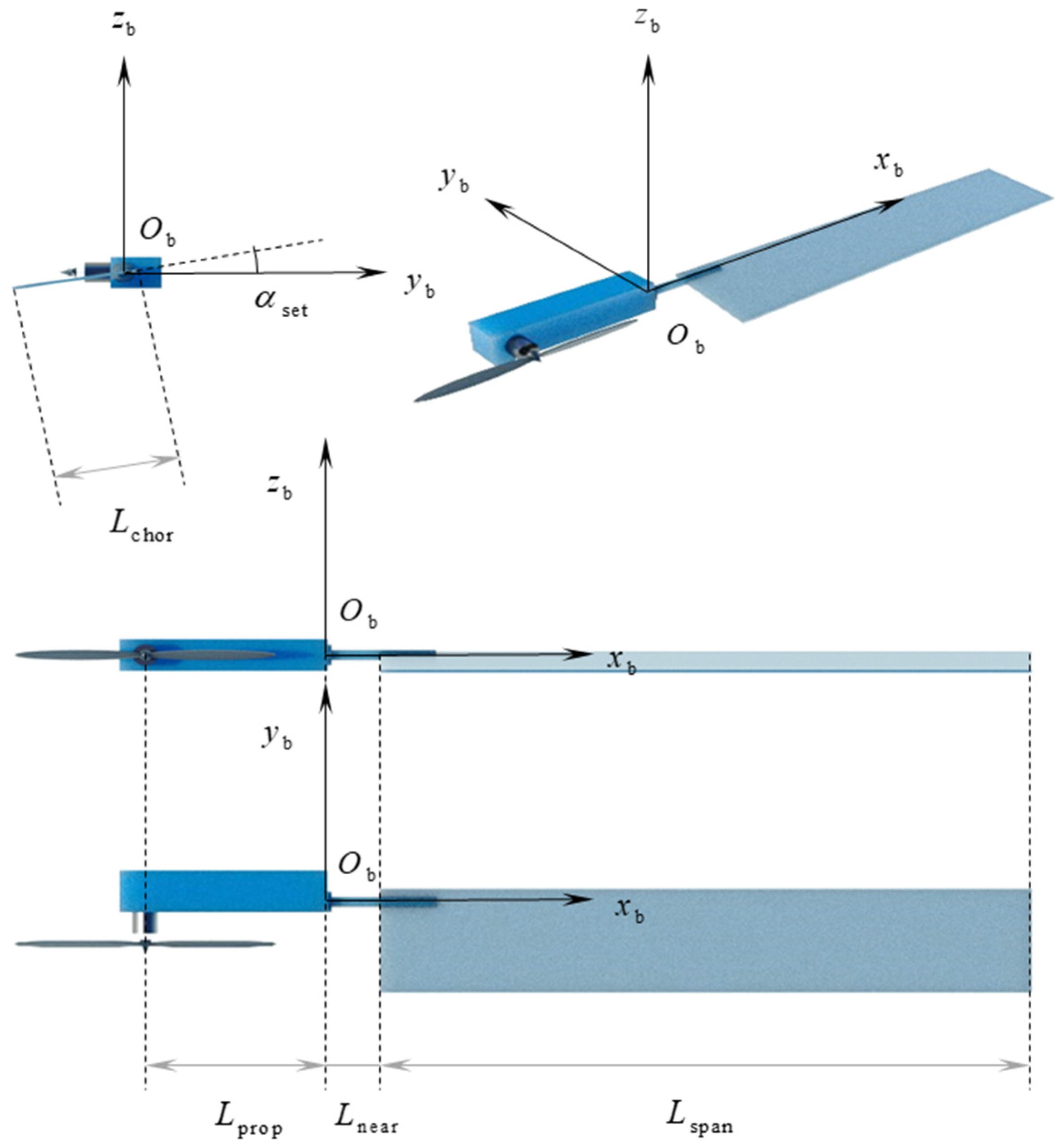
The paper is structured as follows: Chapter 2 presents the configuration and parameters of the single-wing spin flight vehicle and its dynamic model. Chapter 3 derives the ADM, providing detailed derivations of the force and torque domain models and error factor function bounds. Chapter 4 demonstrates the model’s theoretical and practical value through a simulation example. Finally, Chapter 5 discusses the findings and concludes the study. Additionally, we have included a Symbol Table (

Table A1. Abbreviations and nomenclature.

Symbol	Definition	Symbol	Definition
${\mathcal{F}}_{\mathrm{g}}$	$\mathrm{Ground} \mathrm{co-ordinate} \mathrm{system} O_{\mathrm{g}}{x}_{\mathrm{g}}{y}_{\mathrm{g}}{z}_{\mathrm{g}}$	${\mu }_{Fi}\left(t\right)$	$\mu \left(t\right)$$\mathrm{of} F_{\mathrm{A}\mathrm{b}i}$$\mathrm{and} F_{\mathrm{A}\mathrm{T}\mathrm{b}i}$$, i=x,y,z$
${\mathcal{F}}_{\mathrm{b}}$	$\mathrm{Body} \mathrm{co-ordinate} \mathrm{system} O_{\mathrm{b}}{x}_{\mathrm{b}}{y}_{\mathrm{b}}{z}_{\mathrm{b}}$	${\mu }_{Fi\min }$	$\mathrm{Lower} \mathrm{bound} \mathrm{of} {\mu }_{Fi}\left(t\right)$$, i=x,y,z$
$m_{\mathrm{a}}$	Total mass	${\mu }_{Fi\max }$	$\mathrm{Upper} \mathrm{bound} \mathrm{of} {\mu }_{Fi}\left(t\right)$$, i=x,y,z$
${\alpha }_{\mathrm{set}}$	Setting angle	${\lambda }_{Fi}\left(t\right)$	$\lambda \left(t\right)$$\mathrm{of} F_{\mathrm{A}\mathrm{b}i}$$\mathrm{and} F_{\mathrm{A}\mathrm{T}\mathrm{b}i}$$, i=x,y,z$
$L_{\mathrm{span}}$	Wingspan	${\lambda }_{Fi\min }$	$\mathrm{Lower} \mathrm{bound} \mathrm{of} {\lambda }_{Fi}\left(t\right)$$, i=x,y,z$
$L_{\mathrm{chor}}$	Chord length	${\lambda }_{Fi\max }$	$\mathrm{Upper} \mathrm{bound} \mathrm{of} {\lambda }_{Fi}\left(t\right)$$, i=x,y,z$
$L_{\mathrm{near}}$	Distance from the center of mass to the wing’s proximal part	$r_{\mathrm{A}}$	$\mathrm{Position} \mathrm{of} \mathrm{the} \mathrm{point} \mathrm{of} \mathrm{application} \mathrm{of} F_{\mathrm{A}}$ on the wing relative to the center of mass
$L_{\mathrm{prop}}$	Distance from the center of the propeller to the vehicle’s center of mass	$r_{\mathrm{AT}}$	$\mathrm{Position} \mathrm{of} \mathrm{the} \mathrm{point} \mathrm{of} \mathrm{application} \mathrm{of} F_{\mathrm{AT}}$ on the wing relative to the center of mass
$F_{\mathrm{L}}$	Lift	$L_{\mathrm{A}1}$	$\mathrm{Distances} \mathrm{from} \mathrm{the} \mathrm{point} \mathrm{of} \mathrm{application} \mathrm{of} F_{\mathrm{A}}$$\mathrm{on} \mathrm{the} \mathrm{wing} \mathrm{to} \mathrm{the} \mathrm{planes} O_{\mathrm{b}}{y}_{\mathrm{b}}{z}_{\mathrm{b}}$
$F_{\mathrm{D}}$	Drag	$L_{\mathrm{A}2}$	$\mathrm{Distances} \mathrm{from} \mathrm{the} \mathrm{point} \mathrm{of} \mathrm{application} \mathrm{of} F_{\mathrm{A}}$$\mathrm{on} \mathrm{the} \mathrm{wing} \mathrm{to} \mathrm{the} x_{\mathrm{b}}$–axis
$v_{\mathrm{A}}$	Airflow velocity	$L_{\mathrm{AT}1}$	$\mathrm{Distances} \mathrm{from} \mathrm{the} \mathrm{point} \mathrm{of} \mathrm{application} \mathrm{of} F_{\mathrm{AT}}$$\mathrm{on} \mathrm{the} \mathrm{wing} \mathrm{to} \mathrm{the} \mathrm{planes} O_{\mathrm{b}}{y}_{\mathrm{b}}{z}_{\mathrm{b}}$
$m_{\mathrm{pm}}$	Portion of the mass of the propeller relative to the motion of the vehicle	$L_{\mathrm{AT}2}$	$\mathrm{Distances} \mathrm{from} \mathrm{the} \mathrm{point} \mathrm{of} \mathrm{application} \mathrm{of} F_{\mathrm{AT}}$$\mathrm{on} \mathrm{the} \mathrm{wing} \mathrm{to} \mathrm{the} x_{\mathrm{b}}$–axis
$J_i$	$\mathrm{Moments} \mathrm{of} \mathrm{inertia}, i=x,y,z$	${\mu }_{L1}\left(t\right)$	$\mu \left(t\right)$$\mathrm{of} L_{\mathrm{A}1}$$\mathrm{and} L_{\mathrm{AT}1}$
$J_{ij}$	Product of inertia,$ij=xy,yz,xz$	${\mu }_{L1\min }$	$\mathrm{Lower} \mathrm{bound} \mathrm{of} {\mu }_{L1}\left(t\right)$
$J_0$	Inertia matrix	${\mu }_{L1\max }$	$\mathrm{Upper} \mathrm{bound} \mathrm{of} {\mu }_{L1}\left(t\right)$
$F$	Resultant external force	${\mu }_{L2}\left(t\right)$	$\mu \left(t\right)$$\mathrm{of} L_{\mathrm{A}2}$$\mathrm{and} L_{\mathrm{AT}2}$
$M$	Resultant external moment	${\mu }_{L2\min }$	$\mathrm{Lower} \mathrm{bound} \mathrm{of} {\mu }_{L1}\left(t\right)$
$v$	Velocity of center of mass	${\mu }_{L2\max }$	$\mathrm{Upper} \mathrm{bound} \mathrm{of} {\mu }_{L1}\left(t\right)$
$\omega$	Angular velocity relative to the center of mass	$M_{\mathrm{A}}$	Calculation value of aerodynamic torque
$g$	Gravitational acceleration	$M_{\mathrm{AT}}$	True value of aerodynamic torque
$F_{\mathrm{b}}$	Projections of $F$$\mathrm{in} {\mathcal{F}}_{\mathrm{b}}$	${\mu }_{Mi}\left(t\right)$	$\mu \left(t\right)$$\mathrm{of} M_{\mathrm{A}\mathrm{b}i}$$\mathrm{and} M_{\mathrm{A}\mathrm{T}\mathrm{b}i}$$, i=x,y,z$
$M_{\mathrm{b}}$	Projections of $M$$\mathrm{in} {\mathcal{F}}_{\mathrm{b}}$	${\mu }_{Mi\min }$	$\mathrm{Lower} \mathrm{bound} \mathrm{of} {\mu }_{Mi}\left(t\right)$$, i=x,y,z$
$v_{\mathrm{b}}$	Projections of $v$$\mathrm{in} {\mathcal{F}}_{\mathrm{b}}$	${\mu }_{Mi\max }$	$\mathrm{Upper} \mathrm{bound} \mathrm{of} {\mu }_{Mi}\left(t\right)$$, i=x,y,z$
${\omega }_{\mathrm{b}}$	Projections of $\omega$$\mathrm{in} {\mathcal{F}}_{\mathrm{b}}$	${\lambda }_{Mi}\left(t\right)$	$\lambda \left(t\right)$$\mathrm{of} M_{\mathrm{A}\mathrm{b}i}$$\mathrm{and} M_{\mathrm{A}\mathrm{T}\mathrm{b}i}$$, i=x,y,z$
$g_{\mathrm{b}}$	Projections of $g$$\mathrm{in} {\mathcal{F}}_{\mathrm{b}}$	${\lambda }_{Mi\min }$	$\mathrm{Lower} \mathrm{bound} \mathrm{of} {\lambda }_{Mi}\left(t\right)$$, i=x,y,z$
$F_{\mathrm{Pb}}$	$\mathrm{Projections} \mathrm{of} \mathrm{thrust} \mathrm{force} \mathrm{produced} \mathrm{by} \mathrm{the} \mathrm{propeller} \mathrm{in} {\mathcal{F}}_{\mathrm{b}}$	${\lambda }_{Mi\max }$	$\mathrm{Upper} \mathrm{bound} \mathrm{of} {\lambda }_{Mi}\left(t\right)$$, i=x,y,z$
$F_{\mathrm{A}\mathrm{b}}$	$\mathrm{Projections} \mathrm{of} \mathrm{aerodynamic} \mathrm{force} \mathrm{in} {\mathcal{F}}_{\mathrm{b}}$	$p$	Momentum
$M_{\mathrm{Pb}}$	$\mathrm{Projections} \mathrm{of} \mathrm{driving} \mathrm{moment} \mathrm{produced} \mathrm{by} \mathrm{the} \mathrm{propeller} \mathrm{in} {\mathcal{F}}_{\mathrm{b}}$	$L$	Moment of momentum
$M_{\mathrm{A}\mathrm{b}}$	$\mathrm{Projections} \mathrm{of} \mathrm{aerodynamic} \mathrm{moment} \mathrm{in} {\mathcal{F}}_{\mathrm{b}}$	$F_{\mathrm{A}\mathrm{T}\mathrm{b}i \min }$	$\mathrm{Lower} \mathrm{bound} \mathrm{of} F_{\mathrm{A}\mathrm{T}\mathrm{b}i}$$, i=x,y,z$
$S$	Known state	$F_{\mathrm{A}\mathrm{T}\mathrm{b}i \max }$	$\mathrm{Upper} \mathrm{bound} \mathrm{of} F_{\mathrm{A}\mathrm{T}\mathrm{b}i}$$, i=x,y,z$
$t$	Time	$M_{\mathrm{A}\mathrm{T}\mathrm{b}i \min }$	$\mathrm{Lower} \mathrm{bound} \mathrm{of} M_{\mathrm{A}\mathrm{T}\mathrm{b}i}$$, i=x,y,z$
$F_i\left(S\right)$	Calculated component of the aerodynamic force in the $i$ direction for any $S$	$M_{\mathrm{A}\mathrm{T}\mathrm{b}i \max }$	$\mathrm{Upper} \mathrm{bound} \mathrm{of} M_{\mathrm{A}\mathrm{T}\mathrm{b}i}$$, i=x,y,z$
$F_{\mathrm{T}i}\left(t,S\right)$	$\mathrm{Corresponding} \mathrm{true} \mathrm{value} \mathrm{of} F_i\left(S\right)$ at $t$	$T_{\mathrm{s}}$	Simulation duration
$\mu \left(t\right)$	Relative error correction factor function	$\Delta t$	Time step
${\mu }_{\min }$	$\mathrm{Lower} \mathrm{bound} \mathrm{of} \mu \left(t\right)$	$F_{\mathrm{prop}}$	Thrust of propeller
${\mu }_{\max }$	$\mathrm{Upper} \mathrm{bound} \mathrm{of} \mu \left(t\right)$	$M_{\mathrm{prop}}$	Drag torque of propeller
$\lambda \left(t\right)$	Absolute error compensation factor function	${\rho }_{\mathrm{i}\mathrm{g}j}$	$\mathrm{Initial} \mathrm{position} \mathrm{in} {\mathcal{F}}_{\mathrm{g}}$$, j=x,y,z$
${\lambda }_{\min }$	$\mathrm{Lower} \mathrm{bound} \mathrm{of} \lambda \left(t\right)$	${\psi }_{\mathrm{i}}$$, {\theta }_{\mathrm{i}}$$, {\phi }_{\mathrm{i}}$	Initial attitude (Eulerian angle)
${\lambda }_{\max }$	$\mathrm{Upper} \mathrm{bound} \mathrm{of} \lambda \left(t\right)$	$v_{\mathrm{i}\mathrm{g}j}$	$\mathrm{Initial} \mathrm{velocity}{M}_{\mathrm{prop}}$$\mathrm{in} {\mathcal{F}}_{\mathrm{g}}$$, j=x,y,z$
$F_{\mathrm{A}}$	Calculation value of aerodynamic force	${\omega }_{\mathrm{i}\mathrm{b}j}$	$\mathrm{Initial} \mathrm{angular} \mathrm{velocity} \mathrm{in} {\mathcal{F}}_{\mathrm{b}}$$, j=x,y,z$
$F_{\mathrm{AT}}$	True value of aerodynamic force	$v_{\mathrm{a}\mathrm{g}j}$	$\mathrm{Average} \mathrm{airspeed} \mathrm{around} \mathrm{the} \mathrm{vehicle} \mathrm{in} {\mathcal{F}}_{\mathrm{g}}$$, j=x,y,z$

) in Appendix A, which lists each symbol and its definition.

2. Motion Model

2.1. Research Object and Co-Ordinate System

This study considers two primary reference co-ordinate systems: ${\mathcal{F}}_{\mathrm{g}}$ and ${\mathcal{F}}_{\mathrm{b}}$. The Earth-fixed co-ordinate system ${\mathcal{F}}_{\mathrm{g}}$ has its origin, $O_{\mathrm{g}}$, located on the Earth’s surface. The $z_{\mathrm{g}}$–axis points opposite to the gravitational acceleration $\mathit{g}$, while the $x_{\mathrm{g}}$–, $y_{\mathrm{g}}$–, and $z_{\mathrm{g}}$–axes form a right-handed system. Within a limited time and space region, ${\mathcal{F}}_{\mathrm{g}}$ can be treated as an inertial frame, allowing the application of Newton’s laws.

As illustrated in Figure 2, the body-fixed co-ordinate system ${\mathcal{F}}_{\mathrm{b}}$ has its origin, $O_{\mathrm{b}}$, at the vehicle’s center of mass. The $x_{\mathrm{b}}$–, $y_{\mathrm{b}}$–, and $z_{\mathrm{b}}$–axes form a right-handed system aligned with the vehicle’s structure.

The single-wing spin vehicle comprises a wing, battery, motor, electronic speed controller (ESC), and propeller, with a total mass of $m_{\mathrm{a}}$ (Figure 2). The wing, designed as a flat plate airfoil, is mounted at an angle ${\alpha }_{\mathrm{set}}$. It has a rectangular shape with a wingspan $L_{\mathrm{span}}$, a chord length $L_{\mathrm{chor}}$, and a thickness not exceeding 4% of $L_{\mathrm{chor}}$. The center of mass is located on a line $L_{\mathrm{chor}}/8$ from the wing’s leading edge. The distance from the center of mass to the wing’s near-center is $L_{\mathrm{near}}$, where $L_{\mathrm{near}}\ge 0$.

The battery and ESC are enclosed in a rectangular housing with a surface area significantly smaller than the wing. The propeller and motor, mounted on the housing, provide the necessary spin propulsion. The distance from the propeller’s center to the vehicle’s center of mass is $L_{\mathrm{prop}}$.

Table 1. Main parameters of spin flight vehicle.

Parameter	Value	Unit
$m_{\mathrm{a}}$	0.6	kg
$L_{\mathrm{near}}$	0.04	m
$L_{\mathrm{span}}$	0.5	m
$L_{\mathrm{chor}}$	0.1	m
$L_{\mathrm{prop}}$	0.14	m
${\alpha }_{\mathrm{set}}$	π/10	rad
$J_x$	0.0012	kg∙m2
$J_y$	0.0060	kg∙m2
$J_z$	0.0068	kg∙m2

lists the primary parameters of the single-wing spin vehicle.

Figure 3 presents the aerodynamic force analysis of the wing section, with $F_{\mathrm{L}}$ representing lift, $F_{\mathrm{D}}$ denoting drag, and ${\mathit{v}}_{\mathrm{A}}$ indicating airflow velocity.

2.2. Dynamics

The mass of the propeller, relative to the vehicle’s motion, is denoted as $m_{\mathrm{pm}}$. When $m_{\mathrm{pm}}$ is significantly smaller than the total vehicle mass $m_{\mathrm{a}}$ (i.e., $m_{\mathrm{pm}}\ll m_{\mathrm{a}}$), the vehicle can be approximated as a rigid body. The unconstrained motion of a rigid body is referred to as general rigid body motion. Therefore, when $m_{\mathrm{pm}}\ll m_{\mathrm{a}}$, the spin vehicle’s motion can be described using a general rigid body motion model based on Newton’s laws. The vehicle’s dynamic equation is given by:

$$\left.\begin{array}{c}{\dot{\mathit{v}}}_{\mathrm{b}}={\mathit{F}}_{\mathrm{b}}/m_{\mathrm{a}}-{\mathit{\omega }}_{\mathrm{b}}\times {\mathit{v}}_{\mathrm{b}}\\ {\dot{\mathit{\omega }}}_{\mathrm{b}}={\mathit{J}}_0^{-1}{\mathit{M}}_{\mathrm{b}}-{\mathit{J}}_0^{-1}{\mathit{\omega }}_{\mathrm{b}}\times {\mathit{J}}_0{\mathit{\omega }}_{\mathrm{b}}\end{array}\right\}$$

(1)

In Equation (1), ${\mathit{J}}_0$ represents the inertia matrix under the condition $J_{xy}=J_{yz}=J_{zx}=0$. The terms ${\mathit{F}}_{\mathrm{b}}$, ${\mathit{M}}_{\mathrm{b}}$, ${\mathit{v}}_{\mathrm{b}}$, and ${\mathit{\omega }}_{\mathrm{b}}$ denote the projections of the total external force $F$, total external moment $M$, center-of-mass velocity $v$, and angular velocity about the center of mass $\omega$ in the ${\mathcal{F}}_{\mathrm{b}}$ co-ordinate system, respectively.

The external force $F_{\mathrm{b}}$, excluding gravity $m_a{g}_{\mathrm{b}}$, consists of two main components: the thrust force $F_{\mathrm{Pb}}$ generated by the propeller and the aerodynamic force $F_{\mathrm{A}\mathrm{b}}$ due to the vehicle’s relative motion through the air. Similarly, the total moment $M_{\mathrm{b}}$ can be decomposed into the driving moment $M_{\mathrm{Pb}}$ produced by the propeller and the aerodynamic moment $M_{\mathrm{A}\mathrm{b}}$ resulting from aerodynamic interactions. Thus, the equation can be expressed as:

$$\left.\begin{array}{c}{F}_{\mathrm{b}}=F_{\mathrm{Pb}}+F_{\mathrm{A}\mathrm{b}}+m_a{g}_{\mathrm{b}}\\ M_{\mathrm{b}}=M_{\mathrm{Pb}}+M_{\mathrm{A}\mathrm{b}}\end{array}\right\}$$

(2)

3. Domain Model of Aerodynamic

Accurately predicting airflow is challenging due to its inherent complexity, leading to uncertainty in the true aerodynamic forces acting on an aircraft. Consequently, significant discrepancies often arise between actual flight performance and simulation predictions. Relying solely on precise aerodynamic values in current aircraft motion simulations is therefore impractical.

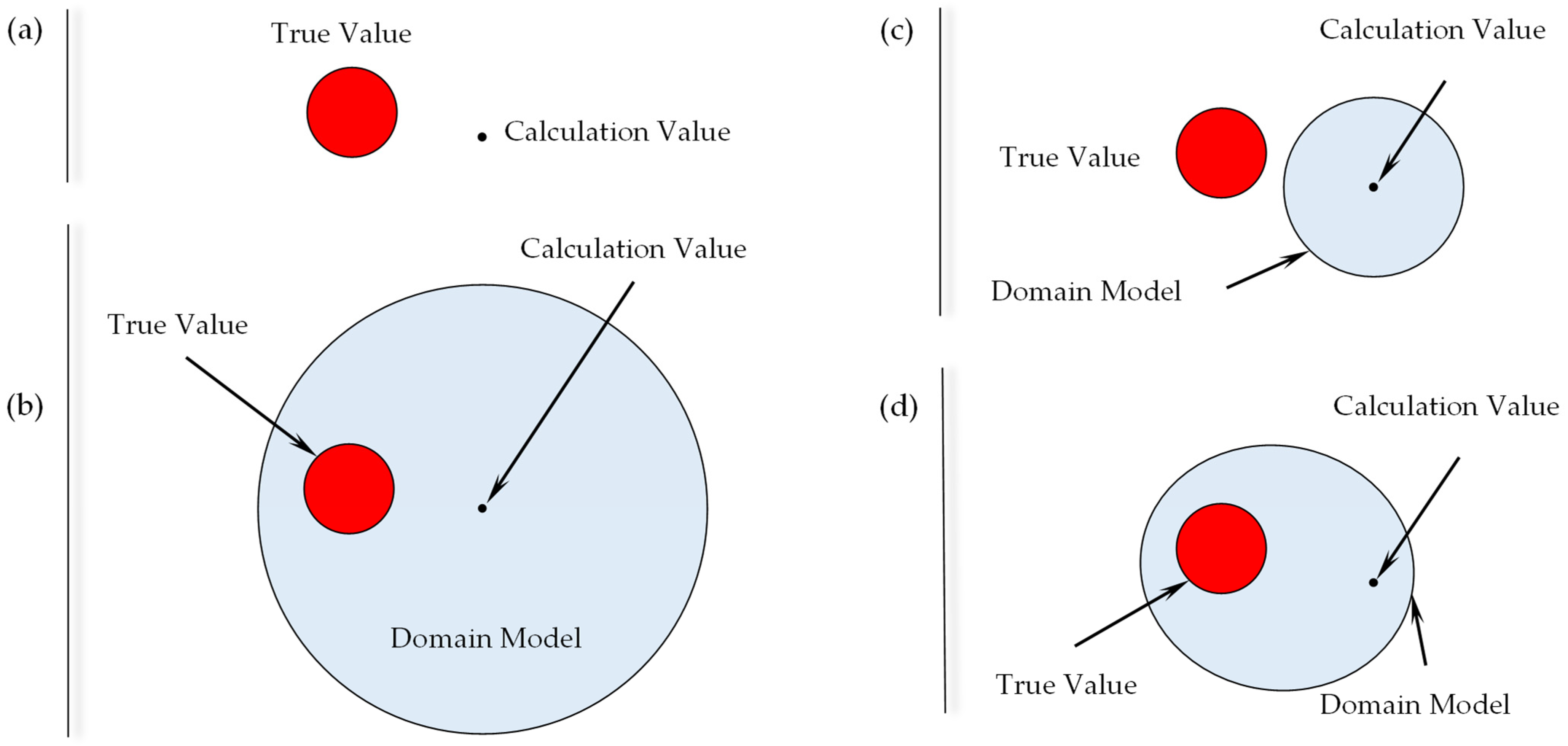
To address the inevitable uncertainties in aerodynamic forces during flight simulations, an ADM is proposed. The ADM uses calculated aerodynamic values as a reference, introducing relative error corrections and absolute error compensations within a defined range. This approach establishes an aerodynamic domain, encompassing all possible true aerodynamic values within that range.

Figure 4 illustrates the principles of the ADM through four sets of diagrams. To further clarify the concepts discussed in this chapter, Figure 5 presents a logical block diagram for reader reference.

3.1. Model Derivation

For any known state $S$, the calculated aerodynamic force component in the $i$ direction is denoted as $F_i\left(S\right)$, and the corresponding true value at time $t$ is denoted as $F_{\mathrm{T}i}\left(t,S\right)$. Real functions $\mu \left(t,S\right)$ and $\lambda \left(t,S\right)$ exist such that:

$$F_{\mathrm{T}i}\left(t,S\right)=\mu \left(t,S\right)F_i\left(S\right)+\lambda \left(t,S\right)$$

(3)

The primary objective is to minimize the gap between the upper and lower bounds of $\mu \left(t,S\right)$ and $\lambda \left(t,S\right)$. To achieve this, constraints are applied. The constraint method is as follows: specifically, for any set of aerodynamic force components $F_i\left(S\right)$ and $F_{\mathrm{T}i}\left(t,S\right)$, there must exist $\mu \in ℝ$, such that:

$$F_{\mathrm{T}i}\left(t,S\right)=\mu F_i\left(S\right)$$

An acceptable upper bound for the relative error factor ${\mu }_{\mathrm{B}}\in \left(0, 1\right)$ is defined, with the general assumption that the closer ${\mu }_{\mathrm{B}}$ is to 0, the better. If $\mu \in \left[1-{\mu }_{\mathrm{B}}, 1+{\mu }_{\mathrm{B}}\right]$, then

$$\left.\begin{array}{c}\mu \left(t,S\right)=\mu \\ \lambda \left(t,S\right)=0\end{array}\right\}$$

If $\mu <1-{\mu }_{\mathrm{B}}$, then

$$\left.\begin{array}{l}\mu \left(t,S\right)=1-{\mu }_{\mathrm{B}}\\ \lambda \left(t,S\right)=F_{\mathrm{T}i}\left(t,S\right)-\left(1-{\mu }_{\mathrm{B}}\right)F_i\left(S\right)\end{array}\right\}$$

If $\mu >1+{\mu }_{\mathrm{B}}$, then

$$\left.\begin{array}{l}\mu \left(t,S\right)=1+{\mu }_{\mathrm{B}}\\ \lambda \left(t,S\right)=F_{\mathrm{T}i}\left(t,S\right)-\left(1+{\mu }_{\mathrm{B}}\right)F_i\left(S\right)\end{array}\right\}$$

If $\mu \to \infty$, then

$$\left.\begin{array}{l}\mu \left(t,S\right)=0\\ \lambda \left(t,S\right)=F_{\mathrm{T}i}\left(t,S\right)\end{array}\right\}$$

For a specific state $S$, for $\forall t\in ℝ$ there must exist ${\mu }_{\min }\left(S\right)\in ℝ$, ${\mu }_{\max }\left(S\right)\in ℝ$, ${\lambda }_{\min }\left(S\right)\in ℝ$, and ${\lambda }_{\max }\left(S\right)\in ℝ$, such that:

$$\left.\begin{array}{c}{\mu }_{\min }\left(S\right)\le \mu \left(t,S\right)\le {\mu }_{\max }\left(S\right)\\ {\lambda }_{\min }\left(S\right)\le \lambda \left(t,S\right)\le {\lambda }_{\max }\left(S\right)\end{array}\right\}$$

where ${\mu }_{\min }\left(S\right)\ge 1-{\mu }_{\mathrm{B}}$ and ${\mu }_{\max }\left(S\right)\le 1+{\mu }_{\mathrm{B}}$. By substituting this inequality into Equation (3), we obtain:

$$\left.\begin{array}{ll}{\mu }_{\min }\left(S\right)F_i\left(S\right)+{\lambda }_{\min }\left(S\right)\le F_{\mathrm{T}i}\left(t,S\right)\le {\mu }_{\max }\left(S\right)F_i\left(S\right)+{\lambda }_{\max }\left(S\right),\hfill & F_i\left(S\right)\ge 0\hfill \\ {\mu }_{\max }\left(S\right)F_i\left(S\right)+{\lambda }_{\min }\left(S\right)\le F_{\mathrm{T}i}\left(t,S\right)\le {\mu }_{\min }\left(S\right)F_i\left(S\right)+{\lambda }_{\max }\left(S\right),\hfill & F_i\left(S\right)<0\hfill \end{array}\right\}$$

(4)

Furthermore, for $\forall S$ there must exist ${\mu }_{\min }\in ℝ$, ${\mu }_{\max }\in ℝ$, ${\lambda }_{\min }\in ℝ$, and ${\lambda }_{\max }\in ℝ$, such that

$$\left.\begin{array}{c}{\mu }_{\min }\le {\mu }_{\min }\left(S\right)\\ {\lambda }_{\min }\le {\lambda }_{\min }\left(S\right)\\ {\mu }_{\max }\ge {\mu }_{\max }\left(S\right)\\ {\lambda }_{\max }\ge {\lambda }_{\max }\left(S\right)\end{array}\right\}$$

(5)

Again, ${\mu }_{\min }\ge 1-{\mu }_{\mathrm{B}}$ and ${\mu }_{\max }\le 1+{\mu }_{\mathrm{B}}$ hold true. By substituting Equation (5) into Equation (4), the relationship between the true aerodynamic force component $F_{\mathrm{T}i}\left(t,S\right)$ and the calculated component $F_i\left(S\right)$ in the $i$ direction is derived as:

$$\left.\begin{array}{cc}{\mu }_{\min }{F}_i\left(S\right)+{\lambda }_{\min }\le F_{\mathrm{T}i}\left(t,S\right)\le {\mu }_{\max }{F}_i\left(S\right)+{\lambda }_{\max },& F_i\left(S\right)\ge 0\hfill \\ {\mu }_{\max }{F}_i\left(S\right)+{\lambda }_{\min }\le F_{\mathrm{T}i}\left(t,S\right)\le {\mu }_{\min }{F}_i\left(S\right)+{\lambda }_{\max },\hfill & F_i\left(S\right)<0\hfill \end{array}\right\}$$

Based on this relationship, the true aerodynamic force component can be expressed as:

$$F_{\mathrm{T}i}\left(t,S\right)\in \left\{x:x=\mu \left(t\right)F_i\left(S\right)+\lambda \left(t\right)\right\}$$

(6)

This forms the ADM, where $\mu \left(t\right)$ is referred to as the relative error correction factor function. It is a continuous function with bounds ${\mu }_{\min }$ and ${\mu }_{\max }$, satisfying:

$$\mu \left(t\right)\in \left\{x:{\mu }_{\min }\le x\le {\mu }_{\max }\right\}$$

This function represents the general relationship between the calculated and true aerodynamic values, accounting for relative errors. Similarly, $\lambda \left(t\right)$ is termed the absolute error compensation factor function. It is also continuous, with bounds ${\lambda }_{\min }$ and, satisfying:

$$\lambda \left(t\right)\in \left\{x:{\lambda }_{\min }\le x\le {\lambda }_{\max }\right\}$$

This function describes the absolute error compensation based on the corrected relative error between the calculated and true aerodynamic values.

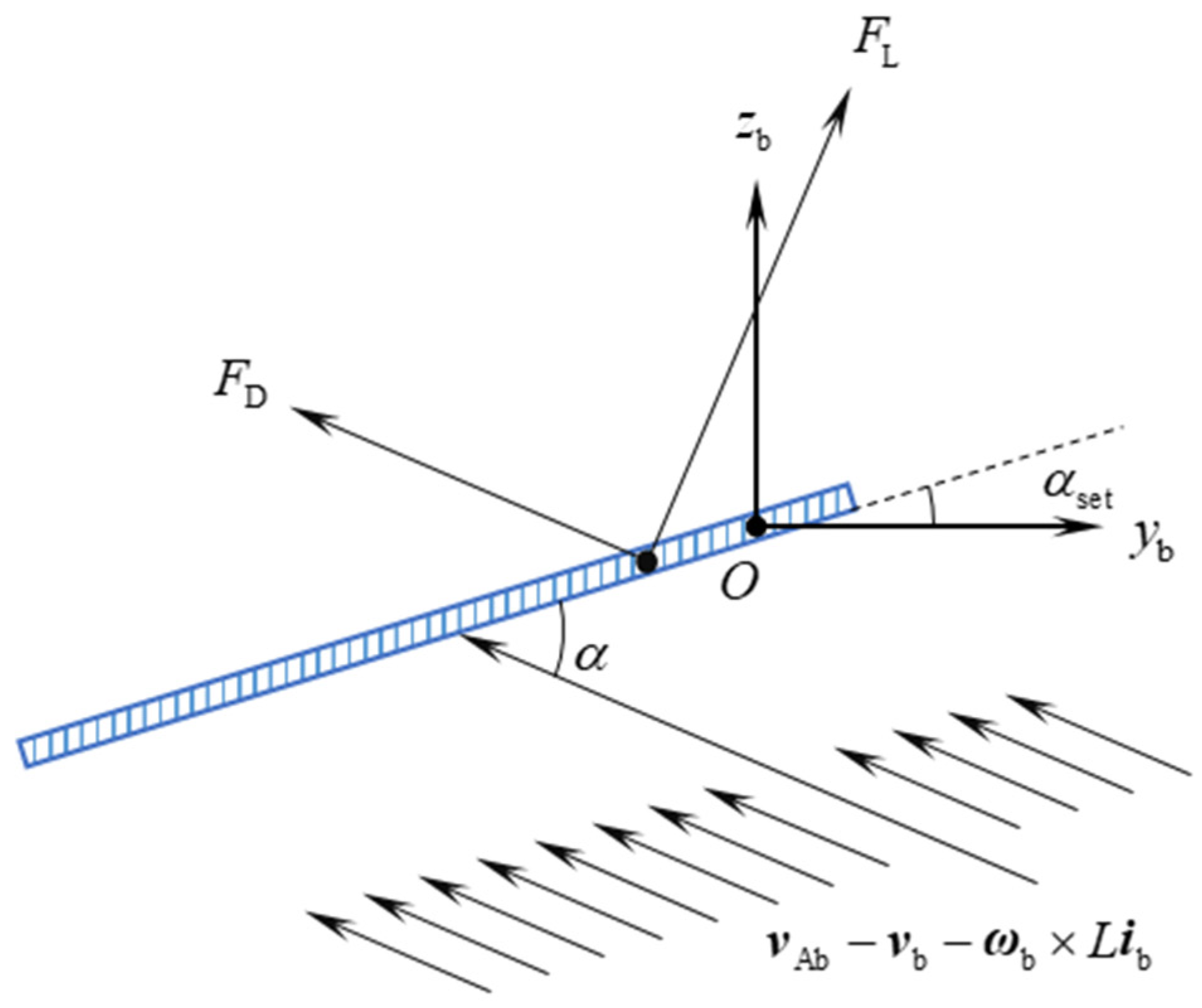
3.2. Force Domain Model

If the aerodynamic forces acting on components other than the wing are neglected, the aerodynamic force components of the spin vehicle’s wing in the $x_{\mathrm{b}}$, $y_{\mathrm{b}}$, and $z_{\mathrm{b}}$ directions, denoted as $F_{\mathrm{A}\mathrm{b}x}$, $F_{\mathrm{A}\mathrm{b}y}$, and $F_{\mathrm{A}\mathrm{b}z}$ can be calculated using the blade element-momentum theory from reference [9].

According to Equation (6), the true aerodynamic force components $F_{\mathrm{AT}}$ of the spin vehicle in the $x_{\mathrm{b}}$, $y_{\mathrm{b}}$, and $z_{\mathrm{b}}$ directions are expressed as:

$$\left.\begin{array}{c}{F}_{\mathrm{A}\mathrm{T}\mathrm{b}x}\in \left\{x:x={\mu }_{Fx}\left(t\right)F_{\mathrm{A}\mathrm{b}x}+{\lambda }_{Fx}\left(t\right)\right\}\\ F_{\mathrm{A}\mathrm{T}\mathrm{b}y}\in \left\{x:x={\mu }_{Fy}\left(t\right)F_{\mathrm{A}\mathrm{b}y}+{\lambda }_{Fy}\left(t\right)\right\}\\ F_{\mathrm{A}\mathrm{T}\mathrm{b}z}\in \left\{x:x={\mu }_{Fz}\left(t\right)F_{\mathrm{A}\mathrm{b}z}+{\lambda }_{Fz}\left(t\right)\right\}\end{array}\right\}$$

(7)

This relationship, represented by Equation (7), defines the aerodynamic force-domain model for the single-wing spin vehicle. Using the previously described constraint method, the lower and upper bounds for the relative error correction factor function and the absolute error compensation factor function can be determined as follows:

$$\left.\begin{array}{c}{\mu }_{Fx}\left(t\right)\in \left\{x:{\mu }_{Fx\min }\le x\le {\mu }_{Fx\max }\right\}\\ {\mu }_{Fy}\left(t\right)\in \left\{x:{\mu }_{Fy\min }\le x\le {\mu }_{Fy\min }\right\}\\ {\mu }_{Fz}\left(t\right)\in \left\{x:{\mu }_{Fz\min }\le x\le {\mu }_{Fz\max }\right\}\\ {\lambda }_{Fx}\left(t\right)\in \left\{x:{\lambda }_{Fx\min }\le x\le {\lambda }_{Fx\max }\right\}\\ {\lambda }_{Fy}\left(t\right)\in \left\{x:{\lambda }_{Fy\min }\le x\le {\lambda }_{Fy\max }\right\}\\ {\lambda }_{Fz}\left(t\right)\in \left\{x:{\lambda }_{Fz\min }\le x\le {\lambda }_{Fz\max }\right\}\end{array}\right\}$$

3.3. Torque Domain Model

The aerodynamic force calculation value $F_{\mathrm{A}}$ and the true value $F_{\mathrm{AT}}$ at the point of application on the wing, relative to the aircraft’s center of mass, are represented by the position vectors $r_{\mathrm{A}}$ and $r_{\mathrm{AT}}$ in the reference frame ${\mathcal{F}}_{\mathrm{b}}$. These vectors can be expressed as:

$$\begin{array}{c}{r}_{\mathrm{A}\mathrm{b}}={\left[\begin{array}{ccc}{L}_{\mathrm{A}1}& - L_{\mathrm{A}2}\cos {\alpha }_{\mathrm{set}}& -L_{\mathrm{A}2}\sin {\alpha }_{\mathrm{set}}\end{array}\right]}^{\mathrm{T}}\\ r_{\mathrm{A}\mathrm{T}\mathrm{b}}={\left[\begin{array}{ccc}{L}_{\mathrm{AT}1}& - L_{\mathrm{AT}2}\cos {\alpha }_{\mathrm{set}}& - L_{\mathrm{AT}2}\sin {\alpha }_{\mathrm{set}}\end{array}\right]}^{\mathrm{T}}\end{array}$$

Here, ${\alpha }_{\mathrm{set}}$ denotes the wing’s setting angle, while $L_{\mathrm{A}1}$ and $L_{\mathrm{A}2}$ represent the distances from the point of application of $F_{\mathrm{A}}$ to the $O_{\mathrm{b}}{y}_{\mathrm{b}}{z}_{\mathrm{b}}$ planes and the $x_{\mathrm{b}}$–axis, respectively. Similarly, $L_{\mathrm{AT}1}$ and $L_{\mathrm{AT}2}$ are the distances from the point of application of $F_{\mathrm{AT}}$ to the same reference planes. Following the approach outlined in Equation (6) and comparing the vectors $r_{\mathrm{AT}}$ and $r_{\mathrm{A}}$, we derive the relationship:

$$\left.\begin{array}{l}{L}_{\mathrm{AT}1}={\mu }_{L1}\left(t\right)L_{\mathrm{A}1}\\ L_{\mathrm{AT}2}={\mu }_{L2}\left(t\right)L_{\mathrm{A}2}\end{array}\right\}$$

(8)

The aerodynamic torque $M_{\mathrm{A}}$ and the true aerodynamic torque $M_{\mathrm{AT}}$ are determined using the expressions $r_{\mathrm{A}}\times F_{\mathrm{A}}$ and $r_{\mathrm{AT}}\times F_{\mathrm{AT}}$, respectively. Thus, in the reference frame ${\mathcal{F}}_{\mathrm{b}}$, they are given by:

$$\left.\begin{array}{l}{M}_{\mathrm{A}\mathrm{b}x}=L_{\mathrm{A}2}\left(\sin {\alpha }_{\mathrm{set}}{F}_{\mathrm{A}\mathrm{b}y}-\cos {\alpha }_{\mathrm{set}}{F}_{\mathrm{A}\mathrm{b}z}\right)\\ M_{\mathrm{A}\mathrm{b}y}=-L_{\mathrm{A}2}\sin {\alpha }_{\mathrm{set}}{F}_{\mathrm{A}\mathrm{b}x}-L_{\mathrm{A}1}{F}_{\mathrm{A}\mathrm{b}z}\\ M_{\mathrm{A}\mathrm{b}z}=L_{\mathrm{A}2}\cos {\alpha }_{\mathrm{set}}{F}_{\mathrm{A}\mathrm{b}x}+L_{\mathrm{A}1}{F}_{\mathrm{A}\mathrm{b}y}\end{array}\right\}$$

(9)

$$\left.\begin{array}{l}{M}_{\mathrm{A}\mathrm{T}\mathrm{b}x}=L_{\mathrm{AT}2}\left(\sin {\alpha }_{\mathrm{set}}{F}_{\mathrm{A}\mathrm{T}\mathrm{b}y}-\cos {\alpha }_{\mathrm{set}}{F}_{\mathrm{A}\mathrm{T}\mathrm{b}z}\right)\\ M_{\mathrm{A}\mathrm{T}\mathrm{b}y}=-L_{\mathrm{AT}2}\sin {\alpha }_{\mathrm{set}}{F}_{\mathrm{A}\mathrm{T}\mathrm{b}x}-L_{\mathrm{AT}1}{F}_{\mathrm{A}\mathrm{T}\mathrm{b}z}\\ M_{\mathrm{A}\mathrm{T}\mathrm{b}z}=L_{\mathrm{AT}2}\cos {\alpha }_{\mathrm{set}}{F}_{\mathrm{A}\mathrm{T}\mathrm{b}x}+L_{\mathrm{AT}1}{F}_{\mathrm{A}\mathrm{T}\mathrm{b}y}\end{array}\right\}$$

(10)

By substituting Equations (7) and (8) into Equation (10) and simplifying, the true aerodynamic torque $M_{\mathrm{AT}}$ in the $x_{\mathrm{b}}$, $y_{\mathrm{b}}$, and $z_{\mathrm{b}}$ directions is obtained as:

$$\left.\begin{array}{ll}{M}_{\mathrm{A}\mathrm{T}\mathrm{b}x}=& {\mu }_{L2}\left(t\right){\mu }_{Fy}\left(t\right)L_{\mathrm{A}2}\sin {\alpha }_{\mathrm{set}}{F}_{\mathrm{A}\mathrm{b}y}-{\mu }_{L2}\left(t\right){\mu }_{Fz}\left(t\right)L_{\mathrm{A}2}\cos {\alpha }_{\mathrm{set}}{F}_{\mathrm{A}\mathrm{b}z}+\\ & {\mu }_{L2}\left(t\right){\lambda }_{Fy}\left(t\right)L_{\mathrm{A}2}\sin {\alpha }_{\mathrm{set}}-{\mu }_{L2}\left(t\right){\lambda }_{Fz}\left(t\right)L_{\mathrm{A}2}\cos {\alpha }_{\mathrm{set}}\\ M_{\mathrm{A}\mathrm{T}\mathrm{b}y}=& -{\mu }_{L2}\left(t\right){\mu }_{Fx}\left(t\right)L_{\mathrm{A}2}\sin {\alpha }_{\mathrm{set}}{F}_{\mathrm{A}\mathrm{b}x}-{\mu }_{L1}\left(t\right){\mu }_{Fz}\left(t\right)L_{\mathrm{A}1}{F}_{\mathrm{A}\mathrm{b}z}-\\ & {\mu }_{L1}\left(t\right){\lambda }_{Fz}\left(t\right)L_{\mathrm{A}1}-{\mu }_{L2}\left(t\right){\lambda }_{Fx}\left(t\right)L_{\mathrm{A}2}\sin {\alpha }_{\mathrm{set}}\\ M_{\mathrm{A}\mathrm{T}\mathrm{b}z}=& {\mu }_{L2}\left(t\right){\mu }_{Fx}\left(t\right)L_{\mathrm{A}2}\cos {\alpha }_{\mathrm{set}}{F}_{\mathrm{A}\mathrm{b}x}+{\mu }_{L1}\left(t\right){\mu }_{Fy}\left(t\right)L_{\mathrm{A}1}{F}_{\mathrm{A}\mathrm{b}y}+\\ & {\mu }_{L1}\left(t\right){\lambda }_{Fy}\left(t\right)L_{\mathrm{A}1}+{\mu }_{L2}\left(t\right){\lambda }_{Fx}\left(t\right)L_{\mathrm{A}2}\cos {\alpha }_{\mathrm{set}}\end{array}\right\}$$

(11)

Since the computed value of $F_{\mathrm{A}\mathrm{b}x}$ is approximately zero, Equations (9) and (11) can be further simplified to

$$\left.\begin{array}{l}{M}_{\mathrm{A}\mathrm{b}x}=L_{\mathrm{A}2}\left(\sin {\alpha }_{\mathrm{set}}{F}_{\mathrm{A}\mathrm{b}y}-\cos {\alpha }_{\mathrm{set}}{F}_{\mathrm{A}\mathrm{b}z}\right)\\ M_{\mathrm{A}\mathrm{b}y}=-L_{\mathrm{A}1}{F}_{\mathrm{A}\mathrm{b}z}\\ M_{\mathrm{A}\mathrm{b}z}=L_{\mathrm{A}1}{F}_{\mathrm{A}\mathrm{b}y}\end{array}\right\}$$

(12)

$$\left.\begin{array}{ll}{M}_{\mathrm{A}\mathrm{T}\mathrm{b}x}=& {\mu }_{L2}\left(t\right){\mu }_{Fy}\left(t\right)L_{\mathrm{A}2}\sin {\alpha }_{\mathrm{set}}{F}_{\mathrm{A}\mathrm{b}y}-{\mu }_{L2}\left(t\right){\mu }_{Fz}\left(t\right)L_{\mathrm{A}2}\cos {\alpha }_{\mathrm{set}}{F}_{\mathrm{A}\mathrm{b}z}+\\ & {\mu }_{L2}\left(t\right){\lambda }_{Fy}\left(t\right)L_{\mathrm{A}2}\sin {\alpha }_{\mathrm{set}}-{\mu }_{L2}\left(t\right){\lambda }_{Fz}\left(t\right)L_{\mathrm{A}2}\cos {\alpha }_{\mathrm{set}}\\ M_{\mathrm{A}\mathrm{T}\mathrm{b}y}=& -{\mu }_{L1}\left(t\right){\mu }_{Fz}\left(t\right)L_{\mathrm{A}1}{F}_{\mathrm{A}\mathrm{b}z}-\\ & {\mu }_{L1}\left(t\right){\lambda }_{Fz}\left(t\right)L_{\mathrm{A}1}-{\mu }_{L2}\left(t\right){\lambda }_{Fx}\left(t\right)L_{\mathrm{A}2}\sin {\alpha }_{\mathrm{set}}\\ M_{\mathrm{A}\mathrm{T}\mathrm{b}z}=& {\mu }_{L1}\left(t\right){\mu }_{Fy}\left(t\right)L_{\mathrm{A}1}{F}_{\mathrm{A}\mathrm{b}y}+\\ & {\mu }_{L1}\left(t\right){\lambda }_{Fy}\left(t\right)L_{\mathrm{A}1}+{\mu }_{L2}\left(t\right){\lambda }_{Fx}\left(t\right)L_{\mathrm{A}2}\cos {\alpha }_{\mathrm{set}}\end{array}\right\}$$

(13)

By comparing Equations (12) and (13), the expressions for the $M_{\mathrm{A}\mathrm{T}\mathrm{b}y}$ and $M_{\mathrm{A}\mathrm{T}\mathrm{b}z}$ components can be written as:

$$\left.\begin{array}{l}{M}_{\mathrm{A}\mathrm{T}\mathrm{b}y}={\mu }_{L1}\left(t\right){\mu }_{Fz}\left(t\right)M_{\mathrm{A}\mathrm{b}y}-{\mu }_{L1}\left(t\right){\lambda }_{Fz}\left(t\right)L_{\mathrm{A}1}-{\mu }_{L2}\left(t\right){\lambda }_{Fx}\left(t\right)L_{\mathrm{A}2}\sin {\alpha }_{\mathrm{set}}\\ M_{\mathrm{A}\mathrm{T}\mathrm{b}z}={\mu }_{L1}\left(t\right){\mu }_{Fy}\left(t\right)M_{\mathrm{A}\mathrm{b}z}+{\mu }_{L1}\left(t\right){\lambda }_{Fy}\left(t\right)L_{\mathrm{A}1}+{\mu }_{L2}\left(t\right){\lambda }_{Fx}\left(t\right)L_{\mathrm{A}2}\cos {\alpha }_{\mathrm{set}}\end{array}\right\}$$

(14)

The sum of the first two terms of $M_{\mathrm{A}\mathrm{T}\mathrm{b}x}$ in Equation (13) is denoted as $M_{1+2}$. To ensure the spin flight vehicle generates sufficient lift, the aerodynamic force $F_{\mathrm{A}\mathrm{b}z}$ must satisfy condition $F_{\mathrm{A}\mathrm{b}z}>0$. When ${\mu }_{Fz}\left(t\right)\ge {\mu }_{Fy}\left(t\right)$, the following inequality holds:

$${\mu }_{L2}\left(t\right){\mu }_{Fz}\left(t\right)M_{\mathrm{A}\mathrm{b}x}\le M_{1+2}\le {\mu }_{L2}\left(t\right){\mu }_{Fy}\left(t\right)M_{\mathrm{A}\mathrm{b}x}$$

When ${\mu }_{Fz}\left(t\right)<{\mu }_{Fy}\left(t\right)$, the inequality remains:

$${\mu }_{L2}\left(t\right){\mu }_{Fy}\left(t\right)M_{\mathrm{A}\mathrm{b}x}<M_{1+2}<{\mu }_{L2}\left(t\right){\mu }_{Fz}\left(t\right)M_{\mathrm{A}\mathrm{b}x}$$

Therefore, the expression for $M_{\mathrm{A}\mathrm{T}\mathrm{b}x}$ can be written as:

$$M_{\mathrm{A}\mathrm{T}\mathrm{b}x}\in \left\{x:x={\mu }_{Mx}\left(t\right)M_{\mathrm{A}\mathrm{b}x}+{\lambda }_{Mx}\left(t\right)\right\}$$

(15)

Here, the lower bound of ${\mu }_{Mx}\left(t\right)$ is the minimum of ${\mu }_{L2}\left(t\right){\mu }_{Fz}\left(t\right)$ and ${\mu }_{L2}\left(t\right){\mu }_{Fy}\left(t\right)$, while the upper bound is the maximum of these two values:

$$\left.\begin{array}{l}{\mu }_{Mx\min }={\mu }_{L2\min }\min \left({\mu }_{Fz\min },{\mu }_{Fy\min }\right)\\ {\mu }_{Mx\max }={\mu }_{L2\max }\max \left({\mu }_{Fz\max },{\mu }_{Fy\max }\right)\end{array}\right\}$$

The lower and upper bounds of ${\lambda }_{Mx}\left(t\right)$ are determined as follows:

If ${\lambda }_{Fy\min }\sin {\alpha }_{\mathrm{set}}\ge {\lambda }_{Fz\max }\cos {\alpha }_{\mathrm{set}}$, then

$${\lambda }_{Mx\min }={\mu }_{L2\min }{L}_{\mathrm{A}2}\left({\lambda }_{Fy\min }\sin {\alpha }_{\mathrm{set}}-{\lambda }_{Fz\max }\cos {\alpha }_{\mathrm{set}}\right)$$

If ${\lambda }_{Fy\min }\sin {\alpha }_{\mathrm{set}}<{\lambda }_{Fz\max }\cos {\alpha }_{\mathrm{set}}$, then

$${\lambda }_{Mx\min }={\mu }_{L2\max }{L}_{\mathrm{A}2}\left({\lambda }_{Fy\min }\sin {\alpha }_{\mathrm{set}}-{\lambda }_{Fz\max }\cos {\alpha }_{\mathrm{set}}\right)$$

If ${\lambda }_{Fy\max }\sin {\alpha }_{\mathrm{set}}\ge {\lambda }_{Fz\min }\cos {\alpha }_{\mathrm{set}}$, then

$${\lambda }_{Mx\max }={\mu }_{L2\max }{L}_{\mathrm{A}2}\left({\lambda }_{Fy\max }\sin {\alpha }_{\mathrm{set}}-{\lambda }_{Fz\min }\cos {\alpha }_{\mathrm{set}}\right)$$

If ${\lambda }_{Fy\max }\sin {\alpha }_{\mathrm{set}}<{\lambda }_{Fz\min }\cos {\alpha }_{\mathrm{set}}$, then

$${\lambda }_{Mx\max }={\mu }_{L2\min }{L}_{\mathrm{A}2}\left({\lambda }_{Fy\max }\sin {\alpha }_{\mathrm{set}}-{\lambda }_{Fz\min }\cos {\alpha }_{\mathrm{set}}\right)$$

The expression for $M_{\mathrm{A}\mathrm{T}\mathrm{b}y}$ and $M_{\mathrm{A}\mathrm{T}\mathrm{b}z}$ in Equation (14) can be written as:

$$\left.\begin{array}{l}{M}_{\mathrm{A}\mathrm{T}\mathrm{b}y}\in \left\{x:x={\mu }_{My}\left(t\right)M_{\mathrm{A}\mathrm{b}y}+{\lambda }_{My}\left(t\right)\right\}\\ M_{\mathrm{A}\mathrm{T}\mathrm{b}z}\in \left\{x:x={\mu }_{Mz}\left(t\right)M_{\mathrm{A}\mathrm{b}z}+{\lambda }_{Mz}\left(t\right)\right\}\end{array}\right\}$$

(16)

The methods for determining the bounds of ${\mu }_{My}\left(t\right)$ and ${\mu }_{Mz}\left(t\right)$ are based on:

$$\left.\begin{array}{l}{\mu }_{My\min }={\mu }_{L1\min }{\mu }_{Fz\min }\\ {\mu }_{My\max }={\mu }_{L1\max }{\mu }_{Fz\max }\\ {\mu }_{Mz\min }={\mu }_{L1\min }{\mu }_{Fy\min }\\ {\mu }_{Mz\max }={\mu }_{L1\max }{\mu }_{Fy\max }\end{array}\right\}$$

The lower and upper bounds of ${\lambda }_{My}\left(t\right)$ are determined as follows:

If ${\lambda }_{Fx\max }\ge 0$ and ${\lambda }_{Fz\max }\ge 0$, then

$${\lambda }_{My\min }=-{\mu }_{L1\max }{\lambda }_{Fz\max }{L}_{\mathrm{A}1}-{\mu }_{L2\max }{\lambda }_{Fx\max }{L}_{\mathrm{A}2}\sin {\alpha }_{\mathrm{set}}$$

If ${\lambda }_{Fx\max }\ge 0$ and ${\lambda }_{Fz\max }<0$, then

$${\lambda }_{My\min }=-{\mu }_{L1\min }{\lambda }_{Fz\max }{L}_{\mathrm{A}1}-{\mu }_{L2\max }{\lambda }_{Fx\max }{L}_{\mathrm{A}2}\sin {\alpha }_{\mathrm{set}}$$

If ${\lambda }_{Fx\max }<0$ and ${\lambda }_{Fz\max }\ge 0$, then,

$${\lambda }_{My\min }=-{\mu }_{L1\max }{\lambda }_{Fz\max }{L}_{\mathrm{A}1}-{\mu }_{L2\min }{\lambda }_{Fx\max }{L}_{\mathrm{A}2}\sin {\alpha }_{\mathrm{set}}$$

If ${\lambda }_{Fx\max }<0$ and ${\lambda }_{Fz\max }<0$, then

$${\lambda }_{My\min }=-{\mu }_{L1\min }{\lambda }_{Fz\max }{L}_{\mathrm{A}1}-{\mu }_{L2\min }{\lambda }_{Fx\max }{L}_{\mathrm{A}2}\sin {\alpha }_{\mathrm{set}}$$

The lower and upper bounds of ${\lambda }_{My}\left(t\right)$ are determined as follows:

If ${\lambda }_{Fx\min }\ge 0$ and ${\lambda }_{Fz\min }\ge 0$, then

$${\lambda }_{My\max }=-{\mu }_{L1\min }{\lambda }_{Fz\min }{L}_{\mathrm{A}1}-{\mu }_{L2\min }{\lambda }_{Fx\min }{L}_{\mathrm{A}2}\sin {\alpha }_{\mathrm{set}}$$

If ${\lambda }_{Fx\min }\ge 0$ and ${\lambda }_{Fz\min }<0$, then

$${\lambda }_{My\max }=-{\mu }_{L1\max }{\lambda }_{Fz\min }{L}_{\mathrm{A}1}-{\mu }_{L2\min }{\lambda }_{Fx\min }{L}_{\mathrm{A}2}\sin {\alpha }_{\mathrm{set}}$$

If ${\lambda }_{Fx\min }<0$ and ${\lambda }_{Fz\min }\ge 0$, then

$${\lambda }_{My\max }=-{\mu }_{L1\min }{\lambda }_{Fz\min }{L}_{\mathrm{A}1}-{\mu }_{L2\max }{\lambda }_{Fx\min }{L}_{\mathrm{A}2}\sin {\alpha }_{\mathrm{set}}$$

If ${\lambda }_{Fx\min }<0$ and ${\lambda }_{Fz\min }<0$, then

$${\lambda }_{My\max }=-{\mu }_{L1\max }{\lambda }_{Fz\min }{L}_{\mathrm{A}1}-{\mu }_{L2\max }{\lambda }_{Fx\min }{L}_{\mathrm{A}2}\sin {\alpha }_{\mathrm{set}}$$

The lower and upper bounds of ${\lambda }_{Mz}\left(t\right)$ are determined as follows:

If ${\lambda }_{Fx\min }\ge 0$ and ${\lambda }_{Fy\min }\ge 0$, then,

$${\lambda }_{Mz\min }={\mu }_{L1\min }{\lambda }_{Fy\min }{L}_{\mathrm{A}1}+{\mu }_{L2\min }{\lambda }_{Fx\min }{L}_{\mathrm{A}2}\cos {\alpha }_{\mathrm{set}}$$

If ${\lambda }_{Fx\min }\ge 0$ and ${\lambda }_{Fy\min }<0$, then

$${\lambda }_{Mz\min }={\mu }_{L1\max }{\lambda }_{Fy\min }{L}_{\mathrm{A}1}+{\mu }_{L2\min }{\lambda }_{Fx\min }{L}_{\mathrm{A}2}\cos {\alpha }_{\mathrm{set}}$$

If ${\lambda }_{Fx\min }<0$ and ${\lambda }_{Fy\min }\ge 0$, then

$${\lambda }_{Mz\min }={\mu }_{L1\min }{\lambda }_{Fy\min }{L}_{\mathrm{A}1}+{\mu }_{L2\max }{\lambda }_{Fx\min }{L}_{\mathrm{A}2}\cos {\alpha }_{\mathrm{set}}$$

If ${\lambda }_{Fx\min }<0$ and ${\lambda }_{Fy\min }<0$, then

$${\lambda }_{Mz\min }={\mu }_{L1\max }{\lambda }_{Fy\min }{L}_{\mathrm{A}1}+{\mu }_{L2\max }{\lambda }_{Fx\min }{L}_{\mathrm{A}2}\cos {\alpha }_{\mathrm{set}}$$

The lower and upper bounds of ${\lambda }_{Mz}\left(t\right)$ are determined as follows:

If ${\lambda }_{Fx\max }\ge 0$ and ${\lambda }_{Fy\max }\ge 0$, then

$${\lambda }_{Mz\max }={\mu }_{L1\max }{\lambda }_{Fy\max }{L}_{\mathrm{A}1}+{\mu }_{L2\max }{\lambda }_{Fx\max }{L}_{\mathrm{A}2}\cos {\alpha }_{\mathrm{set}}$$

If ${\lambda }_{Fx\max }\ge 0$ and ${\lambda }_{Fy\max }<0$, then

$${\lambda }_{Mz\max }={\mu }_{L1\min }{\lambda }_{Fy\max }{L}_{\mathrm{A}1}+{\mu }_{L2\max }{\lambda }_{Fx\max }{L}_{\mathrm{A}2}\cos {\alpha }_{\mathrm{set}}$$

If ${\lambda }_{Fx\max }<0$ and ${\lambda }_{Fy\max }\ge 0$, then

$${\lambda }_{Mz\max }={\mu }_{L1\max }{\lambda }_{Fy\max }{L}_{\mathrm{A}1}+{\mu }_{L2\min }{\lambda }_{Fx\max }{L}_{\mathrm{A}2}\cos {\alpha }_{\mathrm{set}}$$

If ${\lambda }_{Fx\max }<0$ and ${\lambda }_{Fy\max }<0$, then

$${\lambda }_{Mz\max }={\mu }_{L1\min }{\lambda }_{Fy\max }{L}_{\mathrm{A}1}+{\mu }_{L2\min }{\lambda }_{Fx\max }{L}_{\mathrm{A}2}\cos {\alpha }_{\mathrm{set}}$$

Equations (7), (15), and (16) establish the aerodynamic force and torque domain model for the single-wing spin flight vehicle.

3.4. Maximum Momentum and Angular Momentum Model

Based on the theorem of center of mass motion and the moment of momentum theorem relative to the center of mass:

$$\left.\begin{array}{l}{\displaystyle \frac{\mathrm{d}p}{\mathrm{d}t}}=F\\ {\displaystyle \frac{\mathrm{d}L}{\mathrm{d}t}}=M\end{array}\right\}$$

To maximize the momentum and angular momentum of aircraft, both $\left|p+\mathrm{d}p\right|$ and $\left|L+\mathrm{d}L\right|$ must reach their highest values, implying that $\left|p+F\mathrm{d}t\right|$ and $\left|L+M\mathrm{d}t\right|$ must also be maximized. In the ${\mathcal{F}}_{\mathrm{b}}$ co-ordinate system, the projections of $\left|p+F\mathrm{d}t\right|$ and $\left|L+M\mathrm{d}t\right|$ are denoted as $\left|p_{\mathrm{b}}+F_{\mathrm{b}}\mathrm{d}t\right|$ and $\left|L_{\mathrm{b}}+M_{\mathrm{b}}\mathrm{d}t\right|$, respectively. According to Equation (2), we have:

$$\left.\begin{array}{c}\left|p_{\mathrm{b}}+F_{\mathrm{b}}\mathrm{d}t\right|=\left|p_{\mathrm{b}}+F_{\mathrm{Pb}}\mathrm{d}t+F_{\mathrm{A}\mathrm{b}}\mathrm{d}t+m_a{g}_{\mathrm{b}}\mathrm{d}t\right|\\ \left|L_{\mathrm{b}}+M_{\mathrm{b}}\mathrm{d}t\right|=\left|L_{\mathrm{b}}+M_{\mathrm{Pb}}\mathrm{d}t+M_{\mathrm{A}\mathrm{b}}\mathrm{d}t\right|\end{array}\right\}$$

Therefore, when $F_{\mathrm{A}\mathrm{b}}\mathrm{d}t$ is aligned with $p_{\mathrm{b}}+F_{\mathrm{Pb}}\mathrm{d}t+m_a{g}_{\mathrm{b}}\mathrm{d}t$, and $M_{\mathrm{A}\mathrm{b}}\mathrm{d}t$ is aligned with $L_{\mathrm{b}}+M_{\mathrm{Pb}}\mathrm{d}t$ in the same octant, and when both $\left|F_{\mathrm{A}\mathrm{b}}\mathrm{d}t\right|$ and $\left|M_{\mathrm{A}\mathrm{b}}\mathrm{d}t\right|$ are maximized, $\left|p_{\mathrm{b}}+F_{\mathrm{b}}\mathrm{d}t\right|$ and $\left|L_{\mathrm{b}}+M_{\mathrm{b}}\mathrm{d}t\right|$ will also reach their maximum values.

Since $F_{\mathrm{Pb}}\mathrm{d}t$, $m_a{g}_{\mathrm{b}}\mathrm{d}t$, and $M_{\mathrm{Pb}}\mathrm{d}t$ are infinitesimal vectors, the octant in which $p_{\mathrm{b}}$ and $L_{\mathrm{b}}$ lie will be the same as that of $p_{\mathrm{b}}+F_{\mathrm{Pb}}\mathrm{d}t+m_a{g}_{\mathrm{b}}\mathrm{d}t$ and $L_{\mathrm{b}}+M_{\mathrm{Pb}}\mathrm{d}t$. Thus, $F_{\mathrm{A}\mathrm{b}}\mathrm{d}t$ and $p_{\mathrm{b}}$, as well as $M_{\mathrm{A}\mathrm{b}}\mathrm{d}t$ and $L_{\mathrm{b}}$, will remain in the same octant. Additionally, since $p_{\mathrm{b}}=m_{\mathrm{a}}{v}_{\mathrm{b}}$ and $L_{\mathrm{b}}=J_0{\omega }_{\mathrm{b}}$ hold true, it follows that $F_{\mathrm{A}\mathrm{b}}$ and $v_{\mathrm{b}}$, as well as $M_{\mathrm{A}\mathrm{b}}$ and ${\omega }_{\mathrm{b}}$, will also remain in the same octant.

Maximizing $\left|F_{\mathrm{A}\mathrm{b}}\mathrm{d}t\right|$ and $\left|M_{\mathrm{A}\mathrm{b}}\mathrm{d}t\right|$ is, therefore, equivalent to maximizing $\left|F_{\mathrm{A}\mathrm{b}}\right|$ and $\left|M_{\mathrm{A}\mathrm{b}}\right|$. By substituting these into the ADM, it can be concluded that, to generate the maximum momentum and angular momentum for the aircraft, $F_{\mathrm{A}\mathrm{T}\mathrm{b}}$ and $v_{\mathrm{b}}$, as well as $M_{\mathrm{A}\mathrm{T}\mathrm{b}}$ and ${\omega }_{\mathrm{b}}$, must be in the same octant, with both $\left|F_{\mathrm{A}\mathrm{T}\mathrm{b}}\right|$ and $\left|M_{\mathrm{A}\mathrm{T}\mathrm{b}}\right|$ maximized.

From Equations (7), (15), and (16), the methods for determining the upper and lower bounds of the components of $F_{\mathrm{A}\mathrm{T}\mathrm{b}}$ are given by:

$$\begin{array}{c}{F}_{\mathrm{A}\mathrm{T}\mathrm{b}x \max }=\left\{\begin{array}{ll}{\mu }_{Fy\max }{F}_{\mathrm{A}\mathrm{b}x}+{\lambda }_{Fy\max }\hfill & F_{\mathrm{A}\mathrm{b}x}\ge 0\hfill \\ {\mu }_{Fy\min }{F}_{\mathrm{A}\mathrm{b}x}+{\lambda }_{Fy\max }\hfill & F_{\mathrm{A}\mathrm{b}x}<0\hfill \end{array}\right.\\ F_{\mathrm{A}\mathrm{T}\mathrm{b}x \min }=\left\{\begin{array}{ll}{\mu }_{Fx\min }{F}_{\mathrm{A}\mathrm{b}x}+{\lambda }_{Fy\min }\hfill & F_{\mathrm{A}\mathrm{b}x}\ge 0\hfill \\ {\mu }_{Fx\max }{F}_{\mathrm{A}\mathrm{b}x}+{\lambda }_{Fy\min }\hfill & F_{\mathrm{A}\mathrm{b}x}<0\hfill \end{array}\right.\end{array}$$

$$\begin{array}{c}{F}_{\mathrm{A}\mathrm{T}\mathrm{b}y \max }=\left\{\begin{array}{ll}{\mu }_{Fy\max }{F}_{\mathrm{A}\mathrm{b}y}+{\lambda }_{Fy\max }\hfill & F_{\mathrm{A}\mathrm{b}y}\ge 0\hfill \\ {\mu }_{Fy\min }{F}_{\mathrm{A}\mathrm{b}y}+{\lambda }_{Fy\max }\hfill & F_{\mathrm{A}\mathrm{b}y}<0\hfill \end{array}\right.\\ F_{\mathrm{A}\mathrm{T}\mathrm{b}y \min }=\left\{\begin{array}{ll}{\mu }_{Fy\min }{F}_{\mathrm{A}\mathrm{b}y}+{\lambda }_{Fy\min }\hfill & F_{\mathrm{A}\mathrm{b}y}\ge 0\hfill \\ {\mu }_{Fy\max }{F}_{\mathrm{A}\mathrm{b}y}+{\lambda }_{Fy\min }\hfill & F_{\mathrm{A}\mathrm{b}y}<0\hfill \end{array}\right.\end{array}$$

$$\begin{array}{c}{F}_{\mathrm{A}\mathrm{T}\mathrm{b}z \max }=\left\{\begin{array}{ll}{\mu }_{Fz\max }{F}_{\mathrm{A}\mathrm{b}z}+{\lambda }_{Fz\max }\hfill & F_{\mathrm{A}\mathrm{b}z}\ge 0\hfill \\ {\mu }_{Fz\min }{F}_{\mathrm{A}\mathrm{b}z}+{\lambda }_{Fz\max }\hfill & F_{\mathrm{A}\mathrm{b}z}<0\hfill \end{array}\right.\\ F_{\mathrm{A}\mathrm{T}\mathrm{b}z \min }=\left\{\begin{array}{ll}{\mu }_{Fz\min }{F}_{\mathrm{A}\mathrm{b}z}+{\lambda }_{Fz\min }\hfill & F_{\mathrm{A}\mathrm{b}z}\ge 0\hfill \\ {\mu }_{Fz\max }{F}_{\mathrm{A}\mathrm{b}z}+{\lambda }_{Fz\min }\hfill & F_{\mathrm{A}\mathrm{b}z}<0\hfill \end{array}\right.\end{array}$$

Similarly, the methods for determining the upper and lower bounds of the components of $M_{\mathrm{A}\mathrm{T}\mathrm{b}}$ are:

$$\begin{array}{c}{M}_{\mathrm{A}\mathrm{T}\mathrm{b}x \max }=\left\{\begin{array}{ll}{\mu }_{Mx\max }{M}_{\mathrm{A}\mathrm{b}x}+{\lambda }_{Mx\max }\hfill & M_{\mathrm{A}\mathrm{b}x}\ge 0\hfill \\ {\mu }_{Mx\min }{M}_{\mathrm{A}\mathrm{b}x}+{\lambda }_{Mx\max }\hfill & M_{\mathrm{A}\mathrm{b}x}<0\hfill \end{array}\right.\\ M_{\mathrm{A}\mathrm{T}\mathrm{b}x \min }=\left\{\begin{array}{ll}{\mu }_{Mx\min }{M}_{\mathrm{A}\mathrm{b}x}+{\lambda }_{Mx\min }\hfill & M_{\mathrm{A}\mathrm{b}x}\ge 0\hfill \\ {\mu }_{Mx\max }{M}_{\mathrm{A}\mathrm{b}x}+{\lambda }_{Mx\min }\hfill & M_{\mathrm{A}\mathrm{b}x}<0\hfill \end{array}\right.\end{array}$$

$$\begin{array}{c}{M}_{\mathrm{A}\mathrm{T}\mathrm{b}y \max }=\left\{\begin{array}{ll}{\mu }_{My\max }{M}_{\mathrm{A}\mathrm{b}y}+{\lambda }_{My\max }\hfill & M_{\mathrm{A}\mathrm{b}y}\ge 0\hfill \\ {\mu }_{My\min }{M}_{\mathrm{A}\mathrm{b}y}+{\lambda }_{My\max }\hfill & M_{\mathrm{A}\mathrm{b}y}<0\hfill \end{array}\right.\\ M_{\mathrm{A}\mathrm{T}\mathrm{b}y \min }=\left\{\begin{array}{ll}{\mu }_{My\min }{M}_{\mathrm{A}\mathrm{b}y}+{\lambda }_{My\min }\hfill & M_{\mathrm{A}\mathrm{b}y}\ge 0\hfill \\ {\mu }_{My\max }{M}_{\mathrm{A}\mathrm{b}y}+{\lambda }_{My\min }\hfill & M_{\mathrm{A}\mathrm{b}y}<0\hfill \end{array}\right.\end{array}$$

$$\begin{array}{c}{M}_{\mathrm{A}\mathrm{T}\mathrm{b}z \max }=\left\{\begin{array}{ll}{\mu }_{Mz\max }{M}_{\mathrm{A}\mathrm{b}z}+{\lambda }_{Mz\max }\hfill & M_{\mathrm{A}\mathrm{b}z}\ge 0\hfill \\ {\mu }_{Mz\min }{M}_{\mathrm{A}\mathrm{b}z}+{\lambda }_{Mz\max }\hfill & M_{\mathrm{A}\mathrm{b}z}<0\hfill \end{array}\right.\\ M_{\mathrm{A}\mathrm{T}\mathrm{b}z \min }=\left\{\begin{array}{ll}{\mu }_{Mz\min }{M}_{\mathrm{A}\mathrm{b}z}+{\lambda }_{Mz\min }\hfill & M_{\mathrm{A}\mathrm{b}z}\ge 0\hfill \\ {\mu }_{Mz\max }{M}_{\mathrm{A}\mathrm{b}z}+{\lambda }_{Mz\min }\hfill & M_{\mathrm{A}\mathrm{b}z}<0\hfill \end{array}\right.\end{array}$$

To maximize the aircraft’s momentum and angular momentum, the values of $F_{\mathrm{A}\mathrm{T}\mathrm{b}}$ and $M_{\mathrm{A}\mathrm{T}\mathrm{b}}$ should be selected as follows:

$$\begin{array}{c}{F}_{\mathrm{A}\mathrm{T}\mathrm{b}x}=\left\{\begin{array}{ll}{F}_{\mathrm{A}\mathrm{T}\mathrm{b}x \max }\hfill & v_{\mathrm{b}x}\ge 0\hfill \\ F_{\mathrm{A}\mathrm{T}\mathrm{b}x \min }\hfill & v_{\mathrm{b}x}<0\hfill \end{array}\right.\\ F_{\mathrm{A}\mathrm{T}\mathrm{b}y}=\left\{\begin{array}{ll}{F}_{\mathrm{A}\mathrm{T}\mathrm{b}y \max }\hfill & v_{\mathrm{b}y}\ge 0\hfill \\ F_{\mathrm{A}\mathrm{T}\mathrm{b}y \min }\hfill & v_{\mathrm{b}y}<0\hfill \end{array}\right.\\ F_{\mathrm{A}\mathrm{T}\mathrm{b}z}=\left\{\begin{array}{ll}{F}_{\mathrm{A}\mathrm{T}\mathrm{b}z \max }\hfill & v_{\mathrm{b}z}\ge 0\hfill \\ F_{\mathrm{A}\mathrm{T}\mathrm{b}z \min }\hfill & v_{\mathrm{b}z}<0\hfill \end{array}\right.\end{array}$$

(17)

$$\begin{array}{c}{M}_{\mathrm{A}\mathrm{T}\mathrm{b}x}=\left\{\begin{array}{ll}{M}_{\mathrm{A}\mathrm{T}\mathrm{b}x \max }\hfill & {\omega }_{\mathrm{b}x}\ge 0\hfill \\ M_{\mathrm{A}\mathrm{T}\mathrm{b}x \min }\hfill & {\omega }_{\mathrm{b}x}<0\hfill \end{array}\right.\\ M_{\mathrm{A}\mathrm{T}\mathrm{b}y}=\left\{\begin{array}{ll}{M}_{\mathrm{A}\mathrm{T}\mathrm{b}y \max }\hfill & {\omega }_{\mathrm{b}y}\ge 0\hfill \\ M_{\mathrm{A}\mathrm{T}\mathrm{b}y \min }\hfill & {\omega }_{\mathrm{b}y}<0\hfill \end{array}\right.\\ M_{\mathrm{A}\mathrm{T}\mathrm{b}z}=\left\{\begin{array}{ll}{M}_{\mathrm{A}\mathrm{T}\mathrm{b}z \max }\hfill & {\omega }_{\mathrm{b}z}\ge 0\hfill \\ M_{\mathrm{A}\mathrm{T}\mathrm{b}z \min }\hfill & {\omega }_{\mathrm{b}z}<0\hfill \end{array}\right.\end{array}$$

(18)

Equations (17) and (18) represent the maximum momentum and angular momentum models for the aircraft.

4. Simulation

The simulation experiment consists of five cases: one without applying the ADM, labeled as “original”, and four using the ADM and the maximum momentum and angular momentum models, named “case 1”, “case 2”, “case 3”, and “case 4”.

Table 2. ADM simulation parameters.

Parameter	Case 1	Case 2	Case 3	Case 4	Unit
${\mu }_{Fy\min }$$, {\mu }_{Fy\max }$	0.90, 1.10	0.80, 1.20	1.00, 1.00	1.00, 1.00	/
${\mu }_{Fz\min }$$, {\mu }_{Fz\max }$	0.90, 1.10	0.80, 1.20	1.00, 1.00	1.00, 1.00	/
${\mu }_{L1\min }$$, {\mu }_{L1\max }$	0.90, 1.10	0.80, 1.20	1.00, 1.00	1.00, 1.00	/
${\mu }_{L2\min }$$, {\mu }_{L2\max }$	0.90, 1.10	0.80, 1.20	1.00, 1.00	1.00, 1.00	/
${\lambda }_{Fx\min }$$, {\lambda }_{Fx\max }$	0.00, 0.00	0.00, 0.00	−0.59, 0.59	−1.18, 1.18	N
${\lambda }_{Fy\min }$$, {\lambda }_{Fy\max }$	0.00, 0.00	0.00, 0.00	−0.59, 0.59	−1.18, 1.18	N
${\lambda }_{Fz\min }$$, {\lambda }_{Fz\max }$	0.00, 0.00	0.00, 0.00	−0.59, 0.59	−1.18, 1.18	N

provides the boundary values of the error factor functions for cases 1 to 4. The cases are divided into two comparative groups. The first group (“original”, “case 1”, and “case 2”) evaluates the effect of relative error correction factor function boundary changes on simulation results. The second group (“original”, “case 3”, and “case 4”) assesses the impact of absolute error compensation factor function boundary changes. The experiment aims to demonstrate how variations in ADM parameters influence the simulation results of a single-wing spin vehicle and assess its capability in predicting the highest theoretical flight risks.

The simulation represents a single-wing spin vehicle’s takeoff from rest under constant propulsion without additional control. Key parameters include the simulation duration $T_{\mathrm{s}}$, step size $\Delta t$, propeller thrust $F_{\mathrm{prop}}$, propeller air resistance torque $M_{\mathrm{prop}}$, initial position ${\rho }_{\mathrm{i}\mathrm{g}x}$, ${\rho }_{\mathrm{i}\mathrm{g}y}$, ${\rho }_{\mathrm{i}\mathrm{g}z}$, initial attitude in Eulerian angles ${\psi }_{\mathrm{i}}$, ${\theta }_{\mathrm{i}}$, ${\phi }_{\mathrm{i}}$, initial center-of-mass velocity $v_{\mathrm{i}\mathrm{g}x}$, $v_{\mathrm{i}\mathrm{g}y}$, $v_{\mathrm{i}\mathrm{g}z}$, initial angular velocity ${\omega }_{\mathrm{i}\mathrm{b}x}$, ${\omega }_{\mathrm{i}\mathrm{b}y}$, ${\omega }_{\mathrm{i}\mathrm{b}z}$, and average air velocity near the vehicle $v_{\mathrm{a}\mathrm{g}x}$, $v_{\mathrm{a}\mathrm{g}y}$, $v_{\mathrm{a}\mathrm{g}y}$.

Table 3. Simulation parameters of spin flight vehicle.

Parameter	Value	Unit
$T_{\mathrm{s}}$	10	s
$\Delta t$	1 × 10−4	s
$F_{\mathrm{prop}}$	5	N
$M_{\mathrm{prop}}$	0.4	N∙m
${\rho }_{\mathrm{i}\mathrm{g}x}$$, {\rho }_{\mathrm{i}\mathrm{g}y}$$, {\rho }_{\mathrm{i}\mathrm{g}z}$	0, 1, 0	m
${\psi }_{\mathrm{i}}$$, {\theta }_{\mathrm{i}}$$, {\phi }_{\mathrm{i}}$	0, 0, 0	rad
$v_{\mathrm{i}\mathrm{g}x}$$, v_{\mathrm{i}\mathrm{g}y}$$, v_{\mathrm{i}\mathrm{g}z}$	0, 0, 0	m∙s−1
${\omega }_{\mathrm{i}\mathrm{b}x}$$, {\omega }_{\mathrm{i}\mathrm{b}y}$$, {\omega }_{\mathrm{i}\mathrm{b}z}$	0, 0, 0	rad∙s−1
$v_{\mathrm{a}\mathrm{g}x}$$, v_{\mathrm{a}\mathrm{g}y}$$, v_{\mathrm{a}\mathrm{g}z}$	0, 0, 0	m∙s−1

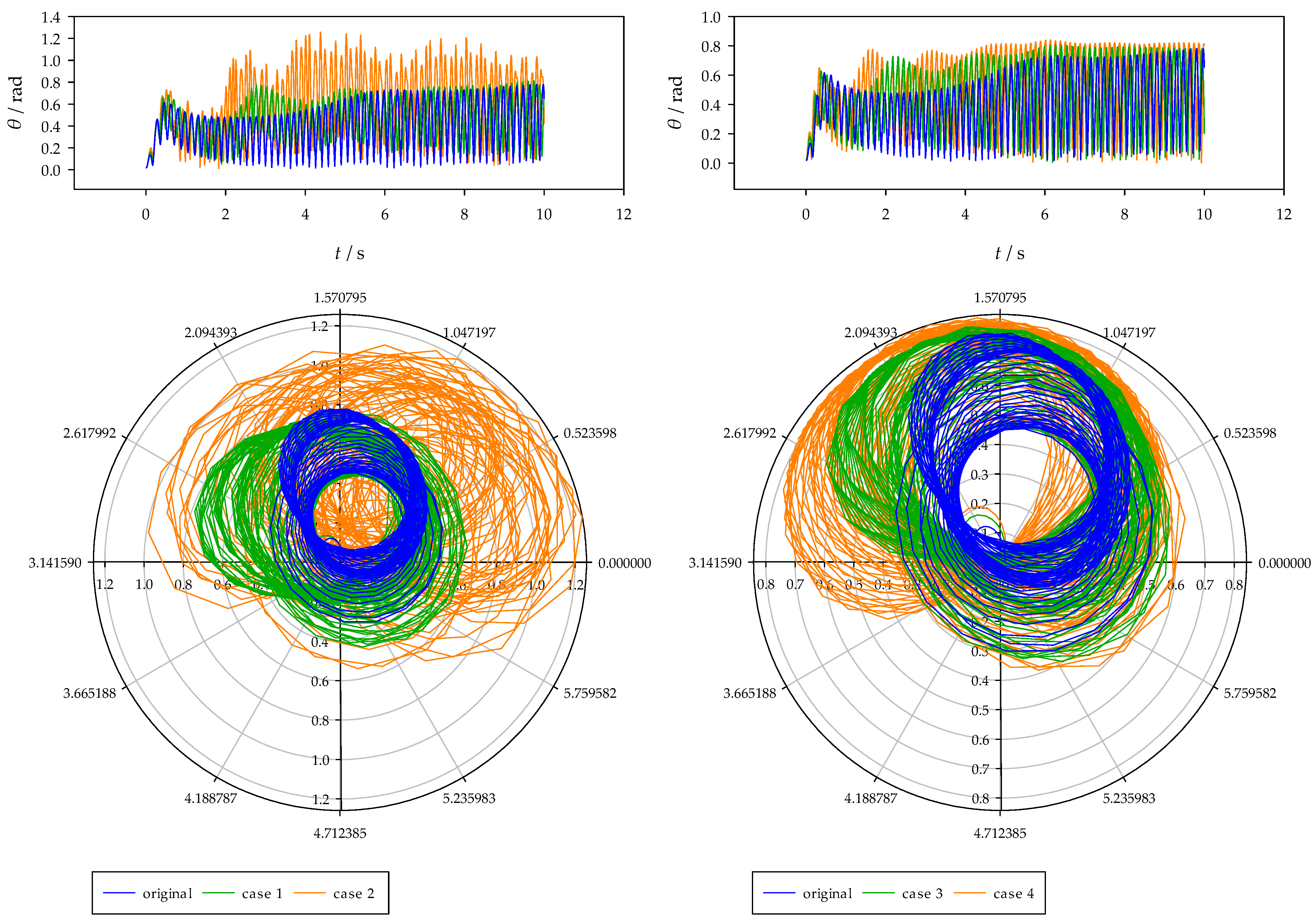
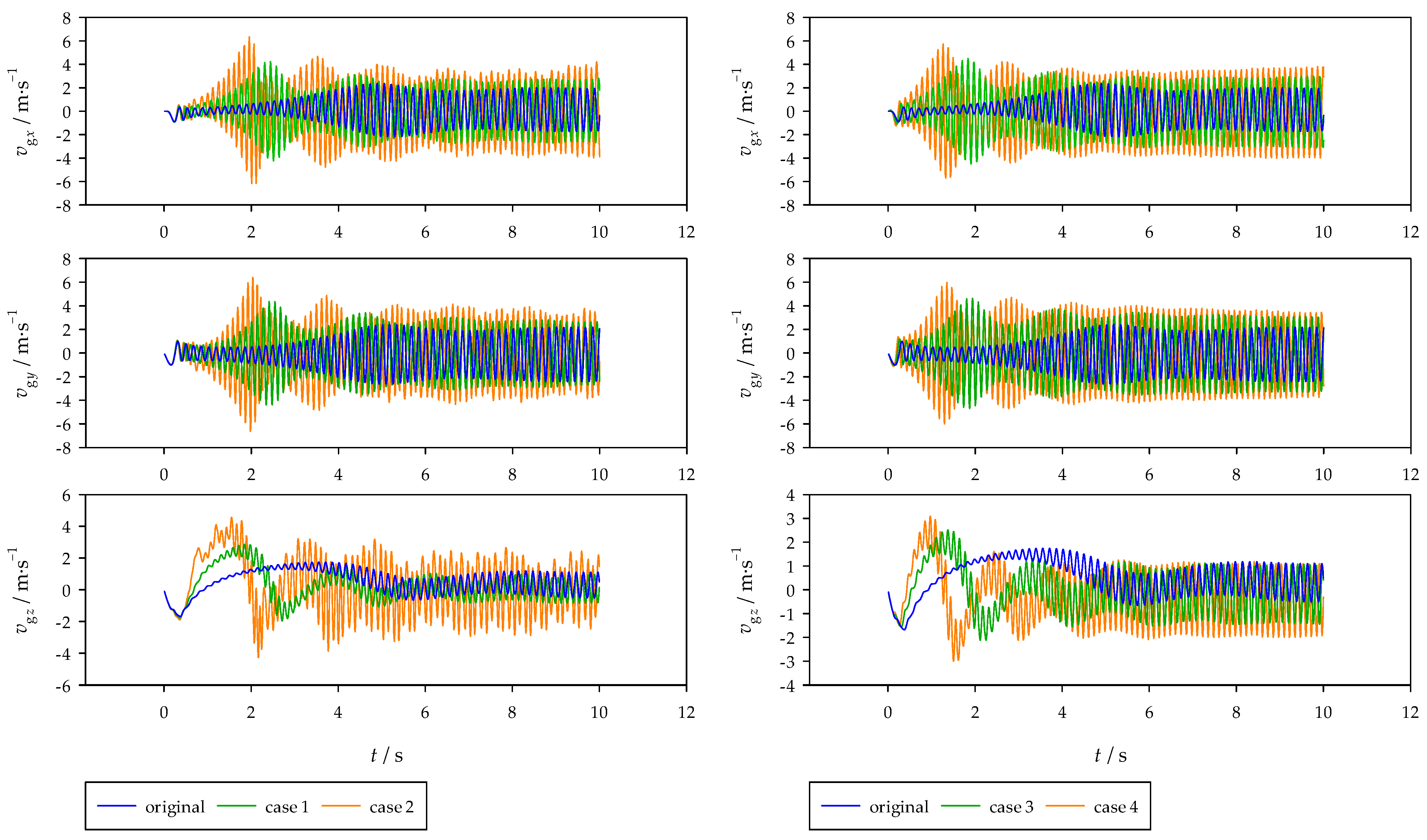
provides specific parameter values. The simulation software was developed in C++ with the code independently written by our laboratory team. The results include four types of motion state data, shown in Figure 6, Figure 7, Figure 8 and Figure 9, illustrating the vehicle’s center-of-mass position, Eulerian angles, center-of-mass velocity, and angular velocity for both groups.

Center-of-Mass Position (Figure 6) Both relative and absolute error factor function boundary changes significantly affect the vehicle’s spatial position. During takeoff, changes in absolute error compensation factor function boundaries have a greater impact on height than relative error correction factor function changes. At 10 s, vehicles in cases 1 and 2 reach approximately 3.2 m, while cases 3 and 4 reach around 0.8 m and −1.9 m, respectively. Vehicles in cases 3 and 4 failed to generate sufficient lift after 5 s, posing significant flight risks. Additionally, relative error correction factor function boundary changes caused greater positional fluctuations, especially during the first 6 s.

Eulerian Angles (Figure 7) Relative and absolute error factor function boundary changes similarly affect the nutation angle, with larger boundary values leading to greater variation. However, the trajectory of the $z_{\mathrm{b}}$–axis intersection on the unit sphere differs notably. In cases 1 and 2, the trajectory centers remain near the circular center, resembling the original case. In contrast, cases 3 and 4 show significant deviations, indicating that absolute error compensation factor function changes substantially impact flight direction, posing higher flight risks. Relative error correction factor function changes mainly increase attitude fluctuation range.

Center-of-Mass Velocity (Figure 8) Both error factor function boundary changes amplify velocity fluctuations, with larger boundary values causing more pronounced fluctuations, particularly in the first 6 s. Peak velocity fluctuations occur at approximately 2.6 s and 2.0 s in cases 1 and 2, and at 1.9 s and 1.3 s in cases 3 and 4. This indicates that increasing boundary values accelerates velocity fluctuation peaks, increasing flight risks. Additionally, absolute error compensation factor function changes significantly reduce the stable average velocity in the $z_{\mathrm{g}}$ direction, whereas relative error correction factor function changes have minimal effect.

Angular Velocity (Figure 9) Both error factor function boundary changes increase angular velocity fluctuation amplitudes and stable mean values of ${\omega }_{\mathrm{b}x}$ and ${\omega }_{\mathrm{b}z}$. Absolute error compensation factor function changes mainly influence angular velocity fluctuations within the first 6 s, while relative error correction factor function changes affect the entire takeoff process. Notably, case 2 shows angular velocity components fluctuating within 15–30 rad/s, indicating instability and elevated flight risks.

Summary Without applying the ADM, the single-wing spin vehicle exhibited the best motion parameter stability and achieved lift-off. Cases 1 and 2 showed that increasing relative error correction factor function boundary values improved the detection of potential attitude and angular velocity risks. Cases 3 and 4 revealed that increasing absolute error compensation factor function boundary values enhanced the identification of center-of-mass position and velocity risks. Consequently, applying the ADM effectively predicts motion state control risks within the defined domain.

A high-performance controller designed using the ADM can mitigate identified risks, ensuring more reliable simulation results. Additionally, the model reduces aerodynamic calculation accuracy requirements, simplifies simulations, and is applicable to most highly dynamic vehicles.

5. Discussion

This paper addresses the reliability of simulation results for single-wing spinning aircraft and the challenge of evaluating flight risks caused by aerodynamic force uncertainties. To tackle these issues, an ADM is proposed, incorporating both relative and absolute aerodynamic errors. The error factor function bounds can be constrained using experimental data or defined as needed. This study provides a detailed derivation of the true aerodynamic forces and moments acting on single-wing spinning aircraft under the ADM, along with a clear method for calculating the error factor function bounds.

A simulation example illustrates the necessity of applying the ADM to single-wing spinning aircraft, demonstrating its ability to predict and warn against flight risks within a defined range. The ADM simulates potential aerodynamic force scenarios within its model domain, effectively representing real-world aerodynamic uncertainties. This significantly enhances the reliability of simulation results and offers a practical means for assessing flight risks.

Furthermore, the ADM shifts the focus from achieving precise aerodynamic calculations to ensuring convergence within a defined domain. Beyond single-wing spinning aircraft, the model is applicable to various high-dynamic aircraft. Future research will explore its practical applications in simulating the motion characteristics of single-wing spinning aircraft.

Using the ADM, high-performance controllers can be designed to mitigate identified risks, ensuring more reliable simulation outcomes. Consequently, the ADM provides a robust foundation for advancing research on aircraft flight dynamics and evaluating control effectiveness. It serves as a valuable tool for enhancing the accuracy and reliability of flight simulations, contributing to future studies on flight behavior and control system validation.