Fundamentals of Innovative Aircraft Heat Exchanger Integration for Hydrogen–Electric Propulsion

Abstract

The potential of utilizing the rejected heat of a fuel cell system to improve the aircraft propulsive efficiency is discussed for various flight conditions. The thermodynamic background of the process and the connection of power consumption in the fan of the ducted propulsor and fuel cell heat are given, and a link between these two components is presented. A concept that goes beyond the known ram heat exchanger is discussed, which outlines the potential benefits of integrating a fan upstream of the heat exchanger. The influence of the fan pressure ratio, flight speed, and altitude, as well as the temperature level of the available fuel cell heat on the propulsive efficiency, is presented. A correlation between the fan pressure ratio, flight speed, and exchangeable fuel cell heat is established, providing a simplified computational approach for evaluating feasible operating conditions within this process. This paper identifies the challenges of heat exchanger integration at International Standard Atmosphere sea level conditions and its benefits for cruise flight conditions. The results show that for a flight Mach number of 0.8 and a fan pressure ratio of 1.5 at a cruising altitude of 11,000 m, the propulsion efficiency increases by approximately 8 percentage points compared to a ducted propulsor without heat utilization. Under sea-level conditions, the concept does not offer any performance advantages over a ducted propulsor. Instead, it exhibits either comparable or reduced propulsive efficiency.

1. Introduction

The aviation industry is expecting a significant increase in commercial air traffic, with forecasts indicating that revenue passenger kilometers are expected to double or even triple by 2050 compared to pre-pandemic levels in 2019, according to the International Civil Aviation Organization (ICAO) Report 2022 [1]. The challenge associated with this growth is that aircraft operations primarily rely on oil-based fuels, resulting in CO₂ and other additional emissions. As the report states, a technology freeze would result in an increase in fuel consumption in the aviation industry by a factor of 2.5 compared to 2019.

The European Commission’s vision, as outlined in the “Fly the Green Deal” report [2], focuses on achieving net-zero CO₂ emissions by 2050. This goal is to be accomplished through several parallel initiatives, including the development of hydrogen infrastructure to enable the utilization of hydrogen as a fuel for aircraft operations at European airports.

Another pathway is to use hydrogen in combination with fuel cells (FCs) in aircraft to provide electricity to the propulsion system, which would dramatically reduce CO₂ emissions in aircraft operations. In this system, hydrogen serves as the chemical energy carrier that is electrochemically converted into electrical power via FCs. The electrical power is supplied to electric motors to generate mechanical power that can be used in a fan or propeller to provide thrust. Adler et al. in [3] mention various hydrogen applications for aircraft, some of which use FCs. Specifically, the research project H2FLY of the German Aerospace Center (DLR) with the HY4 demonstrator, as well as companies like ZeroAvia and Universal Hydrogen, demonstrate the capabilities of using FCs in aircraft.

A challenge in using low-temperature Proton Exchange Membrane Fuel Cells (PEMFCs) is the required cooling system, as they produce a significant amount of heat. Wilberforce et al. state that the generated heat amounts to about 45–60% of the hydrogen energy input [4]. This research also proposes ways of utilizing the heat; however, the only suitable aircraft application seems to be the pre-heating of the reactants.

The work of Heerden et al. [5] elaborates on the challenges of thermal management in the aviation context, focusing on the rising onboard heat loads in aircraft and addressing the high and low ambient temperatures that an aircraft can experience, along with the challenges for the thermal management system. The ram air cooling systems, similar to those proposed by Meredith et al. in [6] and researched in more detail by Becker et al. in [7], are discussed but with an additional puller fan for low flight speeds to enhance airflow through the heat exchanger (HX).

Kellermann et al. [8] focus on an 180-seater passenger aircraft with a hybrid design of gas turbines and electric motors. The HX system in this design is intended to remove the heat generated by the electrical components. Additionally, the off-design of the HX system is focused on fulfilling the demands regarding heat dissipation during take-off. It is also noted that the thermal management system becomes more complex if large batteries or FCs are included in the powertrain. The used HX design is a cross-flow plate-fin HX.

Including an FC as the main energy source of the propulsion system is part of the research provided by Adler et al. in [9]. In this work, a ducted HX without a fan upstream or downstream of the HX is used. The design aims to slow down the incoming airflow with a diffuser to reduce the drag associated with the HX. The research focuses on computational fluid dynamics analysis of the HX for three different flight conditions: take-off, with a flight Mach number of 0.25, and two cruise points, with flight Mach numbers of 0.45 and 0.5. The coolant inlet temperature is fixed at 90 °C. The authors also state that theoretically, some of the thermal energy can be recovered, but the effect depends on the ram pressure. The static pressure at the HX in their work depends solely on the flight Mach number, as no fan is included in the model that could be used to pressurize the airflow through the HX. This utilization concept to recover thermal energy is based on the Brayton cycle, which demands a pressure ratio and additional heat to generate a useful energy output.

In a study by Mark Drela, the low-drag integration of HXs in high-altitude piston-engine aircraft is investigated, focusing on their cooling requirements and the associated installation effects. The research explains the complex interactions between HXs and upstream diffusers, revealing that HXs can mitigate flow separation tendencies in diffusers with high area ratios. The study also examines the impact of duct placement on airflow characteristics. Drela analyzes both front-mounted and aft-mounted airfoil/heat exchanger configurations, each presenting distinct advantages and challenges. The front-mounted configuration may offer superior access to undisturbed airflow but could potentially interfere with the wing aerodynamics. In contrast, the aft-mounted configuration, while benefiting from reduced incoming airflow speeds, may encounter issues related to boundary layer ingestion [10].

In [11], Hübner et al. from the DLR conduct a study on numerical tools and methods for the analysis of HXs in hybrid-electric propulsion concepts. They develop a test case with an isolated ram air HX with integrated diffuser and nozzle segment. Their research compares the Body Force Heat Exchanger method implemented in the DLR-TAU code with OpenFOAM simulations, finding that both approaches yielded qualitatively similar results. A key aspect of the study is the aerodynamic performance analysis of nozzle length variations. The results demonstrate that shorter nozzle lengths improve the overall efficiency.

Insights into different types and designs of HX are given by Shah and Sekulic in [12]. The book provides a comprehensive overview of various HX types, designs, and calculation methods. It covers a wide range of HX configurations, including shell-and-tube, plate, extended surface, and regenerative HXs. The authors present a step-by-step methodology for HX design, allowing readers to follow a structured process from concept to implementation.

Wang et al. in [13] provide a comprehensive overview of surface HXs and their applications in aircraft. Their work presents a historical perspective on surface HXs, focusing particularly on their use for cooling piston engines. As engine power increased over time, the required surface area for heat dissipation has grown substantially, eventually leading to surface HXs covering almost the entire aircraft to meet the cooling demands. Wang et al. [13] note that the primary motivation for using surface HXs is their potential for lower drag compared to ducted HXs.

Scope of the Work

The primary objective of this work is to study the benefits of enhancing the pressure level in the HX section and upcycling the FC heat that occurs for different FC efficiencies. The enhancement of the pressure level is carried out by the fan that is positioned upstream of the HX allowing to increase the static pressure at the HX section. As previously stated, this allows to increase the static pressure level beyond what is achievable with the ramjet effect. This concept of positioning the fan upstream of the HX for an aircraft application is different from what can be found in the literature. Known concepts focus on HX only or HX and puller fan concepts that primarily aim to dissipate a certain amount of heat while only using the advantages of the ramjet effect.

In this work, the combined pressure increase in the HX section, influenced by flight speed and a fan upstream of the HX with different fan pressure ratios, is studied. The pressure loss experienced by the working fluid (the air moving through the propulsor) due to the HX is investigated along with the influence of pressure losses occurring at the intake diffuser, fan, and nozzle. A major influence on HX systems, as stated in [5], is the ambient temperature, particularly at sea level altitude, where the ambient temperature is the highest. This is even more critical when the fan increases the working fluid’s temperature through fan compression. International Standard Atmosphere (ISA) conditions at sea level are simulated to investigate the influence of the fan pressure ratio ($FPR$) and flight speed on the system. Calculations are also carried out at an altitude of 11,000 m to investigate the characteristics of the presented concept under cruise flight conditions.

This work should answer the following questions:

• How does the fan upstream of the HX improve the propulsive efficiency compared to ducted propulsors across different flight conditions?
• What are the advantageous operating parameters (e.g., flight speed, $FPR$) for this system?
• What is the effect considering the air side losses of an HX on the propulsive efficiency compared to an idealized design?

The approach in this paper is to start with a ducted propulsor, incorporating an idealized model of an HX with the intention to first analyze the theoretical performance limits due to heat addition without physical limitations of the HX. In the first part of the results in Section 3, the constraints regarding the pressure losses and temperature level are disregarded. This serves as a reference point for maximum efficiency in the dependency of the available FC heat. Next, the drawbacks of this approach are analyzed and discussed. Finally, a realistic model of the HX is introduced that incorporates the physical limitations. This allows to compare both models and to identify real-world inefficiencies that can be attributed to the HX. This approach allows for a systematic examination and clarification of individual loss mechanisms.

2. Methods

2.1. Proposed Concept

As stated before, the heat generation of PEMFCs is unavoidable since the conversion process from chemical power to electrical power results in a significant amount of heat. This is depicted in Figure 1, where the occurring process heat can be identified and split into two different shares. The proportion that is not removed by the cooling system, i.e., losses in the form of radiation and convection of the FC, is mainly in the form of heat expelled via the exhaust system. The second share must be removed via a cooling system for i.e., a liquid cooling circuit that absorbs the FC heat and transports it to an HX. The exFan project intends to utilize this share of heat absorbed by the cooling system to achieve additional thrust. This is indicated as the purple line in the Sankey diagram of Figure 1.

The concepts found in the literature, which focus on reducing flow velocity, are extended in this work by adding a fan upstream of the HX as shown in Figure 2. The reason for this is the increase in pressure ratio achieved by the fan, which goes beyond the ramjet effect. This increase in the pressure ratio should result in an increase in process efficiency, as the pressure ratio has a direct effect on the thermal efficiency of such a process.

Figure 2 illustrates the whole design of a ducted propulsor equipped with an HX positioned downstream of the fan stage, which for this paper is called the exFan. The configuration shown is divided into segments, beginning with an inlet (Segments 1–2) designed to diffuse the incoming airflow, thus reducing the internal flow velocity while increasing the static pressure of the working fluid.

Following the inlet, the fan stage (Segments 2–3) further increases the total pressure of the working fluid. In the transition duct (Segments 3–4), the flow velocity is further decreased with a slight increase in static pressure. Segments 4–5 locate the HX, which raises the working fluid temperature, thereby increasing its enthalpy. Between Segments 5 and 7, space is reserved for potential future advancements in the project. Finally, in the nozzle (Segments 7–8), static pressure is converted into dynamic pressure to generate thrust.

A well-known application in aviation, utilizing solely the forward motion for compression by using a diffuser followed by a combustor for heat addition, is the ramjet [15]. An idealized representation of the ramjet process is shown as a dashed line in the enthalpy–entropy (h-s) diagram in Figure 3. The exFan concept differs from this approach by incorporating an additional fan stage (Segments 2–3) to increase the pressure ratio of the system. This is shown in Figure 3 as a solid line. This enhancement elevates the static pressure beyond what can be achieved relying only on dynamic pressure as in the conventional ramjet principle.

Differently from the ramjet process, where a combustion process is used to increase the working fluid temperature, exFan uses the rejected heat of an FC to increase the enthalpy of the working fluid. The different heat addition via an HX compared to a combustion process has one major drawback, which is the often greater pressure loss in the working fluid due to the HX. If the pressure losses exceed the benefit of the process, drag is created instead of additional thrust. In Figure 3, this would result in $\Delta h_{{(Inlet+Fan+HX)}_N}$ becoming smaller than $\Delta h_{{(Inlet+Fan)}_N}$.

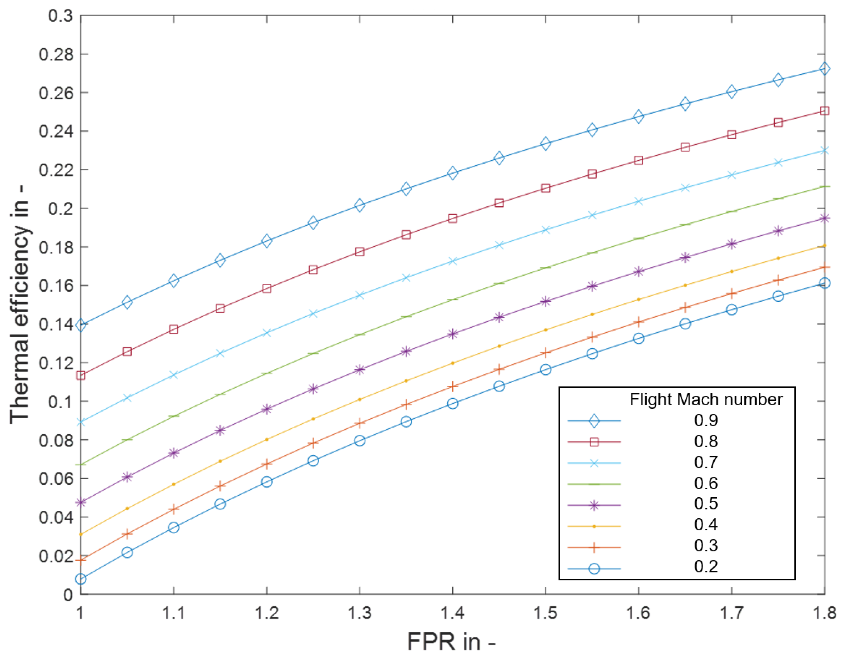
With increasing flight velocity, the available dynamic pressure to be converted into static pressure rises, resulting in higher compression ratios. Since the exFan concept is intended for flight velocities below Mach 0.8, this effect is limited. The incorporated fan stage allows to further increase this compression ratio, resulting in higher thermal efficiencies [16]. Figure 4 shows the thermal efficiency according to Equation (1) plotted versus the $FPR$ with the flight Mach number ${\mathrm{M}}_{0.0}$ as a parameter. The parameter ${\mathrm{M}}_{0.0}$ represents the ram effect, while the $FPR$ stands for the compression by the fan stage. To evaluate the upper limit of the thermal cycle efficiency, the dynamic pressure is fully recovered to a static pressure rise. As shown in Figure 4, there is a benefit to the higher dynamic pressure, represented by higher flight speeds and an increase in $FPR$. For an intended flight speed close to Mach 0.8, the cycle efficiency is approximately 0.12 and can be further enhanced with an increase in $FPR$.

$${\eta }_{th}=1-{\left({\displaystyle \frac{p_{4.0}}{p_{0.0}}}\right)}^{{\displaystyle \frac{\gamma -1}{\gamma }}}$$

(1)

With an increase in $FPR$, the specific work supplied to the working fluid rises. As illustrated in Figure 3, the fan compression raises the enthalpy level, which requires work from the fan by converting mechanical power. The fan is driven by electric motors connected through a transmission gearbox, with the motor drawing its power from the FC. The result is a direct relation between fan compression and the heat from the FC to be dissipated via the HX since the working fluid is not solely used to provide thrust but also to serve as a heat absorbent in the HX.

Figure 5 shows the energy flow path to transfer electric power from the FC via the power converter to the electric motor, where the electric power is converted to mechanical power. This mechanical power can be transmitted to the fan, which converts it and adds energy to the working fluid. Figure 5 illustrates that the components in reality experience losses. While these losses could be incorporated into the model, they are intentionally excluded, as they fall outside the scope of this paper. Consequently, $q_{\mathrm{PC}}$, $q_{\mathrm{EM}}$ and $q_{\mathrm{TM}}$ are set to zero, treating the components as ideal (loss-free) for the purposes of this analysis. Therefore, $\Delta h_{Fan}$ is set equal to $\Delta h_{PC}$. This assumption enables a direct relation of the specific fan work and the associated specific FC power output. It allows to calculate the heat generated in the FC per kilogram of working fluid compressed by the fan, under different operating conditions (temperature, pressure) and set parameters (flight speed, $FPR$). The approach enables the estimation of the share of heat generated by the FC based on its efficiency ${\eta }_{\mathrm{FC}}$. The specific amount of heat converted by the FC is marked as $q_{\mathrm{FC}}$ in Figure 5 and indicates that the heat is transferred from the FC to the HX.

The parameter $FPR$ shown in Equation (2) defines the total pressure ratio of the fan. Equation (2) combined with Equation (3) results in Equation (4), which enables to calculate the total temperature after the fan if the total temperature before is known. These values can be used in Equation (5) to calculate the specific isentropic fan work $\Delta h_{Fan,is}$ needed for certain $FPR$s in an idealized fan stage:

$$FPR={\displaystyle \frac{p_{\mathrm{t}3.0}}{p_{\mathrm{t}2.0}}}$$

(2)

$${\displaystyle \frac{T_{\mathrm{t}3.0}}{T_{\mathrm{t}2.0}}}={\left({\displaystyle \frac{p_{\mathrm{t}3.0}}{p_{\mathrm{t}2.0}}}\right)}^{{\displaystyle \frac{\gamma -1}{\gamma }}}$$

(3)

$$T_{\mathrm{t}3.0}=T_{\mathrm{t}2.0}·{\mathit{FPR}}^{\frac{\gamma -1}{\gamma }}$$

(4)

$$\Delta h_{\mathrm{Fan},\mathrm{is}}=c_{\mathrm{p}}·\left(T_{\mathrm{t}3.0}-T_{\mathrm{t}2.0}\right)=c_{\mathrm{p}}·T_{\mathrm{t}2.0}·\left({\mathit{FPR}}^{\frac{\gamma -1}{\gamma }}-1\right)$$

(5)

The unit of the specific amount of FC heat $q_{\mathrm{FC}}$ can be expressed as $\mathrm{J}/{\mathrm{kg}}_{\mathrm{air}}$, referring to the compressed working fluid that is used as the heat absorbent. When the power needed for compression increases due to higher $FPR$ values, an increased specific amount of heat $q_{\mathrm{FC}}$ is available in the HX for a given overall efficiency value of the FC.

For a simplified and idealized representation, a constant fuel cell efficiency of 50% following [4,14] is assumed. As Sazali et al. outline in [14], around 80% of the heat must be removed by the cooling system. For simplicity, this work assumes that in the FC, hydrogen is either converted into electricity or heat, which is dissipated via the HX. This assumption is reflected by Equation (6):

$${\displaystyle \frac{\Delta h_{\mathrm{Fan}}}{{\eta }_{\mathrm{FC}}}}={\displaystyle \frac{q_{\mathrm{FC}}}{1-{\eta }_{\mathrm{FC}}}}$$

(6)

In Figure 6, the assumption stated in Equation (6) is depicted, and the relation of the fan work and the associated specific amount of heat to be dissipated in the HX is shown. $\Delta h_{\mathrm{Inlet}}$ describes the pressure recovery in the inlet (Segments 1–2), resulting in an increase in static pressure for an isentropic intake diffuser. Three variants of $FPR$, namely $\Delta h_{\mathrm{L}\text{-}\mathrm{FPR}}$ for low $FPR$ compression, $\Delta h_{\mathrm{M}\text{-}\mathrm{FPR}}$ for medium $FPR$ compression, and $\Delta h_{\mathrm{H}\text{-}\mathrm{FPR}}$ for high $FPR$ compression, are marked in Figure 6 for the fan stage. The process is depicted for the three $FPR$ cases, and it is observed that an increase in $FPR$ results in a theoretically more efficient and more effective Brayton cycle. The reason for this lies in the higher compression that results in a higher thermal cycle efficiency and in a rise in the working potential due to the direct interconnection of compression and the rise in addable heat. Therefore, process-wise $FPR$ should be maximized to drive the process efficiency and effectiveness up. So far, this assumption is valid because there is no specification for the temperature level of the available heat. In Section 3.2, the influence of the temperature level is further discussed.

The amount of heat that is available to be transferred to the working fluid is not solely dependent on the $FPR$ but is also the result of the fuel cell efficiency that affects the ratio of heat to electrical energy output. If the FC efficiency changes, it results in an increase (lower ${\eta }_{\mathrm{FC}}$) or decrease (higher ${\eta }_{\mathrm{FC}}$) in the available heat. The amount of heat available influences the working potential of the cycle. Figure 7 graphically demonstrates the influence on the heat conversion of a low-efficiency FC ($q_{\mathrm{FC},\mathrm{LE}}$) in orange, a medium-efficiency FC ($q_{\mathrm{FC},\mathrm{ME}}$) in blue and a high-efficiency FC ($q_{\mathrm{FC},\mathrm{HE}}$) in red, deriving from the associated $\Delta h_{\mathrm{M}\text{-}\mathrm{FPR}}$. The working potential increases with the specific amount of heat available for the exFan process. The influence of the temperature level of the occurring heat is not considered in these assumptions.

2.2. Propulsor Model with an Idealized Heat Exchanger

A MATLAB R2023b model of the exFan propulsor is set up to obtain information about the process and to understand its possible benefits. A rubberized model is used, allowing for flexible sizing based on specified parameters rather than fixed dimensions. The turbomachinery approach to calculate the specific thrust over a range of $FPR$s and flight speeds for various air properties is selected. The system components are modeled with appropriate parameters for the intake diffuser, fan, and nozzle. The values of the parameters can be found in

Table 1. System component parameters [18].

Name	Parameter	Value
$r_{\mathrm{Intake}\text{-}\mathrm{diffuser}}$	Total pressure ratio intake diffuser	0.96
${\eta }_{\mathrm{Fan},\mathrm{poly}}$	Polytropic fan efficiency	0.93
${\eta }_{\mathrm{Nozzle}}$	Nozzle efficiency	0.97

. The idealized HX model in this section does not consider the pressure losses occurring in the HX.

For Segments 1–2, the inlet total pressure ratio, as defined in Equation (7), is employed to determine the properties at station 2. The method follows the approach described by Hill and Peterson in [18] to account for an appropriate reduction in the total pressure in the intake diffuser segment:

$$p_{t2.0}=p_{t1.0}·r_{\mathrm{Intake}\text{-}\mathrm{diffuser}}$$

(7)

In Equation (8), a defined polytropic efficiency is introduced, which allows to calculate different isentropic efficiencies over a range of $FPR$s. This is because the isentropic efficiency decreases with an increase in $FPR$ as described by Saravanamuttoo et al. in [19], while the polytropic efficiency stays constant. The paper focuses on low pressure ratios, implying that the isentropic efficiency changes are only minor but are still considered, as even small temperature changes have a relevant influence on the effectiveness of the HX:

$${\eta }_{\mathrm{Fan},\mathrm{is}}={\displaystyle \frac{{\mathit{FPR}}^{\frac{\gamma -1}{\gamma }}-1}{FP{R}^{\frac{\gamma -1}{{\eta }_{\mathrm{Fan},\mathrm{poly}}·\gamma }}-1}}$$

(8)

Similar to Equation (4) but including the isentropic efficiency, Equation (9) can be formulated to calculate the total temperature after the fan:

$$T_{t3.0}=T_{t2.0}·\left({\displaystyle \frac{FP{R}^{\frac{\gamma -1}{\gamma }}}{{\eta }_{\mathrm{Fan},\mathrm{is}}}}-1\right)$$

(9)

Combining Equation (9) with Equation (5), it is possible to calculate the necessary specific compression work due to the fan incorporating the isentropic fan efficiency. To determine the heat generated in the FC applying a non-idealized fan, the result of Equation (5) must be applied to Equation (6).

Located after the fan, the transition duct is placed in Segments 3–4. The Mach number at station 4, the inlet of the HX, is defined as a control parameter in the model but is kept constant throughout this work. The value can be found in

Table 2. Fixed parameters for the model.

Name	Parameter	Value	Unit
${\mathrm{M}}_{2.0}$	Fan Mach number	0.5 [20]	-
${\mathrm{M}}_{4.0}$	HX inlet Mach number	0.15 [20]	-
$b_{\mathrm{T}}$	HX triangle side length	5	mm
$k_{\mathrm{d}}$	HX surface roughness	0.1	mm

.

The total pressure $p_{\mathrm{t}3.0}$ is known and is identical to $p_{\mathrm{t}4.0}$, as the transition duct is assumed to be loss-free. The total temperature upstream of the HX $T_{\mathrm{t}4.0}$ is identical to $T_{\mathrm{t}3.0}$, as an adiabatic flow process for the transition duct is assumed following the methods of Saravanamuttoo et al. in [19].

The HX is described in more detail in Section 2.3. This allows an idealized view of the concept with component (intake diffuser, fan, and nozzle) losses. In this section, an idealized HX should be described, which does not reduce the total pressure value but increases the total temperature. This is considered with the properties for air, with the heat capacity ratio $\gamma$ and the gas constant $R$ to calculate the specific heat $c_{\mathrm{p}}$. The simple approach follows Equation (10), allowing to calculate the temperature downstream of the idealized HX with a known temperature upstream of the HX, the specific heat of air, and the given amount of heat $q_{\mathrm{FC}}$ from Equation (6) following [21]:

$$q_{\mathrm{FC}}=q_{\mathrm{HX}}=c_{\mathrm{p}}·(T_{\mathrm{t}5.0}-T_{\mathrm{t}4.0})$$

(10)

The nozzle component efficiency is used in Equation (11) to calculate the total pressure at station 8, knowing the parameters downstream of the HX at station 5, which are equal to 7, following the methods described in [18]:

$$p_{\mathrm{t}8.0}={\displaystyle \frac{p_{8.0}}{{\left(1-{\eta }_{\mathrm{nozzle}}·\left(1-{\left(\frac{p_{8.0}}{p_{\mathrm{t}7.0}}\right)}^{\frac{\gamma -1}{\gamma }}\right)\right)}^{\frac{\gamma }{\gamma -1}}}}$$

(11)

The model considers unchoked and choked nozzle exit flows. With the total pressure and the known ambient pressure, it is possible to check if the nozzle pressure ratio ($NPR$), see Equation (12), exceeds the critical pressure ratio ($P{R}_{\mathrm{crit}}$) [16]. If the nozzle pressure ratio is below the critical pressure ratio, the pressure at the nozzle outlet $p_{8.0}$ becomes equal to the ambient pressure $p_{100.0}$, which is equal to $p_{0.0}$ for aircraft flight conditions. In the case of choked flow, $p_{8.0}$ is calculated using Equation (13). An iterative approach is required to determine $p_{8.0}$, as it is not directly available for use in Equation (11). The nozzle is assumed to be adiabatic, resulting in $T_{\mathrm{t}5.0}$ being equal to $T_{\mathrm{t}8.0}$:

$$NPR={\displaystyle \frac{p_{\mathrm{t}8.0}}{p_{100.0}}}$$

(12)

$$p_{8.0}={\displaystyle \frac{p_{\mathrm{t}8.0}}{P{R}_{\mathrm{crit}}}}$$

(13)

Calculating the static temperature at the nozzle exit for a choked flow follows Equation (14) and allows to calculate the nozzle exit speed using Equation (15):

$$T_{8.0}={\displaystyle \frac{T_{\mathrm{t}8.0}}{{\left(P{R}_{\mathrm{crit}}\right)}^{\frac{\gamma -1}{\gamma }}}}$$

(14)

$$v_{8.0}=\sqrt{\gamma ·R·T_{8.0}}$$

(15)

Calculating the static temperature at the nozzle exit for an unchoked flow follows Equation (16) and allows to calculate the nozzle exit speed using Equation (17):

$$T_{8.0}={\displaystyle \frac{T_{\mathrm{t}8.0}}{{\left(\frac{p_{\mathrm{t}8.0}}{p_{100.0}}\right)}^{\frac{\gamma -1}{\gamma }}}}$$

(16)

$$v_{8.0}=\sqrt{2·c_{\mathrm{p}}·(T_{\mathrm{t}8.0}-T_{8.0})}$$

(17)

With the known nozzle exit properties, it is possible to determine Equation (18):

$${\rho }_{8.0}={\displaystyle \frac{p_{8.0}}{R·T_{8.0}}}$$

(18)

The pressure loss in the HX is neglected for this part of the calculation, allowing to investigate the upper efficiency limit of the process. Equation (23) serves as the fundamental expression to compute the propulsive efficiency, while Equations (19)–(22) are employed to derive its specific form. Equation (19) describes the propulsive power with the net thrust (${\mathrm{F}}_{\mathrm{N}}$) and $v_{0.0}$ as the flight speed. In Equation (20), the total fan power is calculated with the specific fan work and the mass flow of the working fluid entering the ducted propulsor, which is equal to the mass flow of the nozzle exit. No friction on the shaft is assumed; therefore, the shaft power $P_{\mathrm{shaft}}$ is equal to the fan power $P_{\mathrm{Fan}}$. The continuity Equation (21) allows the mass flow to be calculated from the nozzle outlet area, the nozzle outlet velocity, and the density at the nozzle outlet. Equation (22) is the momentum equation rearranged to calculate the nozzle exit area for a given ${\mathrm{F}}_{\mathrm{N}}$.

The parameters with the index “i” in Equations (20)–(23) vary depending on the selected process. There are two processes which are compared: the ducted propulsor and the exFan. The ducted propulsor process, labeled as “no HX”, does not introduce additional heat into the working fluid. In contrast, the exFan process, denoted as “HX”, involves additional heat generated by the FC. To compare these processes, the propulsive power is kept constant, and both are analyzed using a rubberized model approach:

$$P_{\mathrm{av}}={\mathrm{F}}_{\mathrm{N}}·v_{0.0}$$

(19)

$$P_{{\mathrm{shaft}}_{\mathrm{i}}}=P_{{\mathrm{Fan}}_{\mathrm{i}}}=\Delta h_{\mathrm{Fan}}·{\dot{m}}_{8.0i}$$

(20)

$${\dot{m}}_{8.0i}=A_{8.0\mathrm{i}}·v_{8.0\mathrm{i}}·{\rho }_{8.0\mathrm{i}}$$

(21)

$$A_{8.0\mathrm{i}}={\displaystyle \frac{{\mathrm{F}}_{\mathrm{N}}}{{\rho }_{8.0\mathrm{i}}·\left(v_{8.0\mathrm{i}}^2-v_{0.0}·v_{8.0\mathrm{i}}\right)-\left(p_{8.0\mathrm{i}}-p_{0.0}\right)}}$$

(22)

$$\begin{array}{c}\hfill {\eta }_{\mathrm{prop}}={\displaystyle \frac{P_{\mathrm{av}}}{P_{{\mathrm{Fan}}_{\mathrm{i}}}}}={\displaystyle \frac{{\mathrm{F}}_{\mathrm{N}}·v_{0.0}}{\Delta h_{\mathrm{Fan}}·{\dot{m}}_{8.0i}}}={\displaystyle \frac{{\mathrm{F}}_{\mathrm{N}}·v_{0.0}}{\Delta h_{\mathrm{Fan}}·A_{8.0\mathrm{i}}·v_{0.0}·{\rho }_{8.0\mathrm{i}}}}=\\ \hfill ={\displaystyle \frac{v_{0.0}·\left({\rho }_{8.0\mathrm{i}}·\left(v_{8.0\mathrm{i}}^2-v_{0.0}·v_{8.0\mathrm{i}}\right)-\left(p_{8.0i}-p_{0.0}\right)\right)}{\Delta h_{\mathrm{Fan}}·v_{8.0\mathrm{i}}·{\rho }_{8.0\mathrm{i}}}}\end{array}$$

(23)

Equation (23) enables the calculation of the propulsive efficiency based on the flight speed, the ambient pressure, the specific work performed in the fan, the air properties, and velocity at the nozzle exit.

2.3. The Non-Idealized HX Model with Pressure Loss

This section focuses on the pressure loss in the HX $\Delta p_{\mathrm{HX}}$ that is immanent when forcing a fluid through an HX. For a ducted propulsor with HX, this pressure loss occurring within the process causes a reduction in the propulsive efficiency, compared to the model described in Section 2.2 that neglects the HX pressure loss. The model used in this section is the same as in Section 2.2 but additionally incorporates the HX as a function with a constant wall temperature ($T_{\mathrm{w}}$) as depicted in Figure 8, and a constant HX inflow Mach number (${\mathrm{M}}_{4.0}$). The assumed HX inflow Mach number is proportional to the speed of the working fluid into the HX air channels.

The red square in Figure 9 marks the area of the HX at station 4 that covers a mass flow rate equivalent of 1 ${\mathrm{kg}}_{\mathrm{air}}/\mathrm{s}$ ingested and depends on the parameters at the inlet of the HX. The dotted red square indicates that the necessary area for this specific airflow is not constant, as the model accounts for varying $FPR$s and flight Mach numbers, leading to different HX inlet area values at station 4. The model accepts different values for the HX inlet Mach numbers (${\mathrm{M}}_{4.0}$) and flight altitude, but both values influence the size of the marked HX inlet area.

The specific ingestion area is referred to as the area to mass flow rate ratio ($AMR$) with the unit [$\left({\mathrm{m}}^2\mathrm{s}\right)/{\mathrm{kg}}_{\mathrm{air}}$] described in Equation (24). The chosen triangle side length ($b_{\mathrm{T}}$), which is found in Figure 9, enables to calculate the number of equilateral triangles that cover the computed inlet area ($AMR$) and is an essential value to calculate the length ($h_{\mathrm{HX}}$) of the HX because it defines the wetted area of the HX channels. The triangular channels shall model a plate and fin HX.

For a specific expression of the area that ingests the working fluid, refer to Equation (21). This equation is reformulated into Equation (24) to describe the $AMR$, which can be calculated with the density and flow velocity of the working fluid at station 4 or with the given inputs shown in Figure 9 at the inlet, as well as the additionally known air properties ($R$, $c_{\mathrm{p}}$):

$$AM{R}_{4.0}={\displaystyle \frac{A_{4.0}}{{\dot{m}}_{4.0}}}={\displaystyle \frac{1}{{\rho }_{4.0}·v_{4.0}}}={\displaystyle \frac{p_{4.0}}{R·T_{4.0}}}·{\displaystyle \frac{1}{\sqrt{2·c_{\mathrm{p}}·(T_{\mathrm{t}4.0}-T_{4.0})}}}$$

(24)

The $AMR$ is used to calculate the Specific Number of Channels ($SNC$) and is given by the ratio of $AMR$ to the area spanned by the equilateral triangle with the specified side length $b_{\mathrm{T}}$ shown in Equation (25). $SNC$ is required to calculate the HX length $h_{\mathrm{HX}}$ using Equation (30) via the required HX surface area $A_{\mathrm{HX},\mathrm{spec}}$ (Equation (29)):

$$SN{C}_{4.0}={\displaystyle \frac{AM{R}_{4.0}}{\frac{b_{\mathrm{T}}^2·\sqrt{3}}{4}}}$$

(25)

The HX function in the model uses the approach of [12,22] to calculate the values needed to exchange the amount of specific heat occurring in the FC. Different from the idealized approach, the temperature level of the heat and the working fluid temperature are considered with this function. For simplicity, the HX surface temperature $T_{\mathrm{w}}$ is assumed to be constant along the length of the HX, representing the temperature at which heat is available for transfer to the working fluid. This approach focuses solely on the heat transfer from the HX surface to the air, disregarding the previous heat transfer from the FC to the HX but acknowledging the amount of heat generated in the FC. An overview of the function is given in Figure 10 and in the following Equations (26)–(30). Important to mention is the fact that Equation (27) is only applicable to fully developed turbulent flow in ducts and is only partially valid for HXs. The inputs to the function from the heat side are only the wall temperature and the amount of specific heat that must be dissipated. Combining the information about the HX inlet temperature, HX inlet pressure, HX inlet Mach number, and the amount of heat that must be dissipated for the specific amount of mass flow rate yields the averaged HX values of velocity, kinematic viscosity, thermal conductivity, temperature, pressure, and heat transfer coefficient (HTC). The function is not explicitly solvable, and therefore, an iterative approach is set up:

$$R{e}_d={\displaystyle \frac{v_{\mathrm{HX},\mathrm{m}}·D_{\mathrm{h}}\left(b_{\mathrm{T}}\right)}{{\nu }_{\mathrm{m}}}}$$

(26)

$$N{u}_{\mathrm{m}}=0.0214·\left(R{e}_d^{0.8}-100\right)·P{r}^{0.4}·\left(1+{\left({\displaystyle \frac{D_{\mathrm{h}}\left(b_{\mathrm{T}}\right)}{h_{\mathrm{HX}}}}\right)}^{{\displaystyle \frac{2}{3}}}\right)·{\left({\displaystyle \frac{T_{\mathrm{HX},\mathrm{m}}}{T_{\mathrm{w}}}}\right)}^{0.45}$$

(27)

$${\alpha }_{\mathrm{m}}={\displaystyle \frac{N{u}_{\mathrm{m}}·{\lambda }_{\mathrm{air},\mathrm{m}}}{D_{\mathrm{h}}\left(b_{\mathrm{T}}\right)}}$$

(28)

The averaged HTC (${\alpha }_{\mathrm{m}}$) calculated with Equation (28) is used to compute the required surface area $A_{\mathrm{HX},\mathrm{spec}}$ for the specific amount of heat $q_{\mathrm{FC}}$ that is specified to be generated by compressing 1 ${\mathrm{kg}}_{\mathrm{air}}/\mathrm{s}$ with the fan using Equation (29). The previous calculated $SNC$ value, combined with the triangle perimeter value, allows the calculation of the HX length using Equation (30):

$$A_{\mathrm{HX},\mathrm{spec}}={\displaystyle \frac{q_{\mathrm{FC}}}{{\alpha }_{\mathrm{m}}·(T_{\mathrm{w}}-T_{\mathrm{HX},\mathrm{m}})}}$$

(29)

$$h_{\mathrm{HX}}={\displaystyle \frac{A_{\mathrm{HX},\mathrm{spec}}}{3·b_{\mathrm{T}}·SN{C}_{4.0}}}$$

(30)

For the computation of the pressure loss through the HX, the explicit approximation of the Colebrook–White equation by Zanke [23] is chosen, which allows to estimate the friction factor ${\zeta }_{\mathrm{pl}}$ with Equation (31) for $R{e}_d$ > 2300. The calculation of the friction factor requires to define the surface roughness $k_{\mathrm{d}}$; this value was set to 0.1 mm. The resulting pressure loss is calculated with Equation (32), which results in the total pressure after the HX at station 5:

$${\displaystyle \frac{1}{\sqrt{{\zeta }_{\mathrm{pl}}}}}=-2log\left[{\displaystyle \frac{2.7{(logR{e}_d)}^{1.2}}{R{e}_d}}+{\displaystyle \frac{k/d}{3.71}}\right]$$

(31)

$$\Delta p_{\mathrm{HX}}={\displaystyle \frac{1}{2}}·{\displaystyle \frac{{\rho }_{\mathrm{m}}·{v_{\mathrm{HX},\mathrm{m}}}^2·{\zeta }_{\mathrm{pl}}·h_{\mathrm{HX}}}{D_{\mathrm{h}}\left(b_{\mathrm{T}}\right)}}$$

(32)

Figure 10 is a schematic that summarizes inputs and outputs used in the HX function. It displays the required inputs in purple, which are “$T_{\mathrm{t}}$ in” ($T_{\mathrm{t}4.0}$), “$p_{\mathrm{t}}$ in” ($p_{\mathrm{t}4.0}$), HX inlet Mach number (${\mathrm{M}}_{4.0}$), HX triangle side length ($b_{\mathrm{T}}$), HX surface temperature ($T_{\mathrm{w}}$), HX friction factor (${\zeta }_{\mathrm{pl}}$) and the heat from the FC $q_{\mathrm{FC}}$. The constant parameters in orange are the Prandtl number $Pr$, gas constant $R$, and heat capacity ratio $\gamma$ of air, which are implemented in the HX function. The outputs in green are “$T_{\mathrm{t}}$ out” ($T_{\mathrm{t}5.0}$) and “$p_{\mathrm{t}}$ out” ($p_{\mathrm{t}5.0}$). The calculations carried out within the function are highlighted with blue boxes.

3. Results

3.1. Results Without Heat Exchanger Pressure Losses

Figure 11 depicts the propulsive efficiencies plotted versus FPRs [1.05 to 1.8] with the flight Mach number as parameter [0.2, 0.5, 0.8]. Subplots Figure 11a–c vary the FC efficiencies [0.75, 0.5, 0.25]. A value of 0.15 is chosen for the HX inlet Mach number because it allows a fair trade-off between the HX size and loss of working fluid pressure in the HX, which is discussed in more detail in Section 3.3. The value for the triangle side length $b_{\mathrm{T}}$ is set to 5 mm for all calculations. Both values and the used fan Mach number ${\mathrm{M}}_{2.0}$ of 0.5 are defined in Table 2.

The exFan process in Figure 11 can be identified with the solid lines compared to the ducted propulsor without heat utilization, which is drawn with dashed lines. Comparing Figure 11a–c, it can be observed that the propulsive efficiencies increase when the FC efficiencies decrease. The lower the fuel cell efficiency, the more heat has to be rejected, which lets the propulsive efficiency increase. This is counterintuitive but valid because the overall efficiency is not investigated but rather the propulsive efficiency. As a matter of fact, the overall efficiency would shrink with lower fuel cell efficiency but, if accounted for, it would obscure the advantages of this process, not allowing it to be investigated clearly. This work focuses on the utilization of the occurring heat, and with more heat, the propulsive efficiency rises. This allows the conclusion that low-efficiency power generation can be counteracted with this type of heat rejection.

As shown in Figure 11, all cases have in common that with an increase in flight speed, the propulsive efficiency increases. The difference between the “HX” and the “no HX” cases increase simultaneously to propulsive efficiency increase with flight Mach number for the HX cases. This is primarily attributable to the ramjet effect that allows to utilize the oncoming airflow. The reason behind this is the increase in thermal efficiency due to the increase in the pressure ratio $p_{4.0}$ to $p_{0.0}$. Another outcome is that a very low $FPR$ is not beneficial because of the pressure losses of the working fluid that must be overcome for the intake diffuser and the nozzle, which ultimately reduces the utilizable total pressure at the nozzle exit. Figure 11c, with a flight Mach number of 0.8 including an HX, shows that even a propulsive efficiency above 100% is possible with this process, which is the result of considering the available heat from the FC as free. While the input energy via the fan is kept constant, a change in the FC efficiency leads to an increase in the heat energy occurring in the FC. This heat energy can be utilized in the exFan, which ultimately allows the level of propulsive efficiency to be raised to these elevated values.

A variation in altitude [0 m and 11,000 m] results in insignificant changes. Therefore, the results in Figure 11 are only shown for an altitude of 11,000 m.

3.2. Drawback of the Idealized Process

In the idealized case, the HX does not regard the temperature difference between the working fluid and the HX surface. However, this temperature difference is physically unavoidable to achieve the required heat exchange to occur as Equation (33) from [21] reveals. Furthermore, the idealized case does not obey the second law of thermodynamics, which defines that heat cannot spontaneously transfer from a lower-temperature body to a higher-temperature one as Rudolf Clausius stated [24]:

$$\dot{Q}=A · \alpha · \Delta T$$

(33)

The diagrams in Figure 12 shows the static air temperatures of the working fluid upstream $T_{4.0}$ and downstream $T_{5.0}$ of the HX for a selected range of $FPR$s over a range of flight Mach numbers. The fuel cell efficiency ${\eta }_{\mathrm{FC}}$ is assumed to be 50% for all cases. A temperature of 90 °C (363.15 K) for the HX surface is assumed due to the low operating temperatures of low-temperature PEMFCs and is indicated as a red dashed line. The difference between Figure 12c,d and Figure 12e,f is the ambient temperature and the range of flight Mach numbers. Figure 12c,d are computed for low ambient temperature under ISA conditions at an altitude of 11 km for flight Mach numbers 0.5 to 0.9. Figure 12e,f show the results at sea level for flight Mach numbers 0.1 to 0.3. It graphically demonstrates the drawback of the thermodynamic approach without considering the physical boundaries. While in Figure 12d the temperature downstream of the HX does not exceed the HX surface temperature, Figure 12f shows that it becomes physically unfeasible for increased $FPR$ values to exchange all the occurring heat at sea level altitude under ISA conditions. The reason for this is the fan compression, which increases the working fluid temperature as shown in Figure 6, thereby reducing the temperature difference between the HX surface and the working fluid. The subsequent heat addition for the idealized process disregards this limitation, resulting in working fluid temperatures that exceed the surface temperature of the HX. The selection of $FPR$ values for Figure 12e,f, is linked to the results in Section 3.3.2, which show that $FPR$ values above certain levels are not beneficial for the process. When the results of Figure 12f are investigated, it reveals that an $FPR$ above 1.6 is not feasible with an HX surface temperature of 90 °C. Under these conditions, the working fluid is not able to absorb the occurring FC heat for the given ambient temperatures of 288 K. Increasing the surface temperature of the HX is indeed possible and allows raising the $FPR$ limit to higher values but reveals that the HX surface temperature physically limits $FPR$ for this process. Another influence that can be observed in Figure 12c,e is that an increase in the flight Mach number, while holding the Mach number at the HX inlet constant, results in a higher working fluid temperature at station 4. This can be attributed to the higher absolute value in dynamic pressure.

3.3. Results Including HX Pressure Loss

The results of the model are shown in Figure 13 and Figure 14. They display the results of propulsive efficiency with an assumed fuel cell efficiency ${\eta }_{\mathrm{FC}}$ of 50%. In both figures, the values for the HX surface temperatures of $T_{\mathrm{w}}$ [60, 90, 120] °C are chosen. The temperature level of 120 °C is chosen because sources indicate that this is a complex but achievable limit for LT-PEMFCs in terms of the operating temperature level [25,26]. Another way to increase the temperature level in the heat exchanger is to use a more sophisticated thermal management system as discussed in more detail by Kösters et al. in [27]. The assumed HX inlet Mach number is set to 0.15, which is estimated to be a reasonable trade-off between the occurring pressure loss $\Delta p_{\mathrm{HX}}$ and the cross-sectional area of the HX inlet, indicated as $D_{\mathrm{HX}}$ in Figure 15. This value falls within the range reported in the work of [20] and is selected based on an evaluation of performance and geometric constraints, which are not further detailed in this work.

In Figure 13, the ISA conditions at an altitude of 11,000 m are assumed and two distinct flight Mach numbers [0.5; 0.8] over a range of $FPR$s [1.05 to 1.8] are computed. The calculated results are intended to characterize the possible cruise performance parameters and to ensure that they correspond to the realistic operating conditions for aircraft in the specified altitude and Mach number range.

In Figure 14, the ISA conditions at sea level altitude are assumed, and two flight Mach numbers [0.2; 0.5] over a range of $FPR$s [1.05 to 1.8] are computed. The results are intended to represent parameters close to the ground (e.g., take-off).

Figure 12. Altitude influence on the working fluid temperature upstream (c,e) and downstream (d,f) of the HX with respect to flight speed, $FPR$, and the occurring FC heat. (a) is intended to represent the location of the results before the HX and (b) after the HX. ISA conditions for the ambient temperature are assumed. (a) is located in the first column of the graphic, indicating the position of the results from (c,e). Similarly, (b) is located in the second column with (d,f). The associated legend for (c–f) is located in sector (g).

Figure 12. Altitude influence on the working fluid temperature upstream (c,e) and downstream (d,f) of the HX with respect to flight speed, $FPR$, and the occurring FC heat. (a) is intended to represent the location of the results before the HX and (b) after the HX. ISA conditions for the ambient temperature are assumed. (a) is located in the first column of the graphic, indicating the position of the results from (c,e). Similarly, (b) is located in the second column with (d,f). The associated legend for (c–f) is located in sector (g).

The exFan process can be identified with the solid lines compared to the ducted propulsor, which is drawn with dashed lines. In the ducted propulsor system without heat utilization, calculating HX pressure loss is unnecessary, as no such loss occurs. Therefore, the results for the ducted propulsor are the same as those in Figure 11.

3.3.1. Influence of HX Surface Temperature at 11,000 m Altitude

All results show benefits in the upcycling of the occurring heat in direct comparison to the ducted propulsor without heat utilization. Comparing Figure 13a–c, a positive behavior for a flight Mach number of 0.5 can be identified, which is primarily a result of the temperature difference between the working fluid and HX surface ($T_{\mathrm{w}}$), which is already high due to the elevated altitude of 11,000 m that offers very low ambient temperatures. As $FPR$ increases, results with lower $T_{\mathrm{w}}$ demonstrate a slightly faster decline in propulsive efficiency compared to those with higher $T_{\mathrm{w}}$. For a flight Mach number of 0.8, the trend is similar, except for the result with a low HX surface temperature shown in Figure 13a. The temperature difference $\Delta T$ between the HX surface and working fluid appears to be too low for the higher $FPR$ values, resulting in a decrease in propulsive efficiency due to greater pressure losses.

Figure 13. Propulsive efficiency at 11 km altitude with pressure loss in HX for HX surface temperatures of [60 °C (a), 90 °C (b) and 120 °C (c)] compared to a ducted propulsor marked as “no HX”. The associated legend for (a–c) is located in quadrant (d).

Figure 13. Propulsive efficiency at 11 km altitude with pressure loss in HX for HX surface temperatures of [60 °C (a), 90 °C (b) and 120 °C (c)] compared to a ducted propulsor marked as “no HX”. The associated legend for (a–c) is located in quadrant (d).

3.3.2. Influence of HX Surface Temperature at Sea Level Altitude

Figure 14 presents the results of the propulsive efficiency under ISA conditions at sea level altitude. All results indicate that the exFan process has no benefit for operations near the ground compared to the ducted propulsor. For an HX surface temperature $T_{\mathrm{w}}$ of 60 °C, as in Figure 14a, and an HX surface temperature $T_{\mathrm{w}}$ of 90 °C, as in Figure 14b, the propulsive efficiency is generally lower for the exFan compared to the ducted propulsor. The exFan variant with a temperature $T_{\mathrm{w}}$ of 120 °C, as shown in Figure 14c, exhibits a similar behavior to the ducted propulsor at a low flight Mach number of 0.2, particularly when the $FPR$ value remains below 1.5. For an increased flight Mach number of 0.5, this similarity in propulsive efficiency between the exFan and the ducted propulsor remains consistent up to an $FPR$ of approximately 1.3. Beyond this threshold, the propulsive efficiencies of the two systems begin to diverge, with the exFan system experiencing a reduction in propulsive efficiency.

Figure 14. Propulsive efficiency at sea level altitude with pressure loss in HX for HX surface temperatures of [60 °C (a), 90 °C (b) and 120 °C (c)] compared to a ducted propulsor marked as “no HX”. The associated legend for (a–c) is located in quadrant (d).

Figure 14. Propulsive efficiency at sea level altitude with pressure loss in HX for HX surface temperatures of [60 °C (a), 90 °C (b) and 120 °C (c)] compared to a ducted propulsor marked as “no HX”. The associated legend for (a–c) is located in quadrant (d).

3.4. Influence Factors on the Heat Exchanger Size

The length of the HX is determined by the amount of heat necessary to dissipate, the temperature difference $\Delta T$ between the working fluid and the HX surface ($T_{\mathrm{w}}$) and the HTC. Section 3.2 reveals the influences on the temperature of the working fluid. Due to the increase in $FPR$ and flight speed, the temperature difference $\Delta T$ decreases. With an increase in $FPR$ the occurring specific heat in the FC increases. Equation (29) shows that the surface area required to dissipate a certain amount of heat is influenced by all those factors. An increase in $q_{\mathrm{FC}}$ results in more surface area, and an increase in $\Delta T$ reduces the required surface area. Both factors have an influence on the length $h_{\mathrm{HX}}$as shown in the upper path of Figure 15.

The HTC is influenced by the Mach number of the working fluid in the HX. Lower Mach numbers in the HX reduce the HTC. To maintain constant mass flow while reducing the HX inlet Mach number, a larger HX inlet area is required, which results in an increase in $D_{\mathrm{HX}}$, as illustrated on the lower path in Figure 15. However, increasing the Mach number of the working fluid at the HX entrance—or equivalently increasing the flow velocity—leads to higher pressure losses in the working fluid due to wall friction. As shown in Equation (32), pressure loss scales with the square of velocity, potentially causing pressure losses that outweigh the benefits of an increase in HTC.

Figure 15. HX length and width influences due to various parameters of the model.

Figure 15. HX length and width influences due to various parameters of the model.

4. Discussion

The results presented in Figure 11, Figure 13 and Figure 14 show the relationship between flight speed, $FPR$ and propulsive efficiency in the exFan concept. Figure 11 demonstrates that propulsive efficiency increases with higher flight Mach numbers when disregarding the effects of HX pressure losses. The propulsive efficiency is further enhanced by the availability of additional free heat energy from the FC as a result of lower FC efficiency as demonstrated by Figure 11a–c. At 50% FC efficiency, this trend persists even when the HX pressure loss is taken into account as shown in Figure 13. However, Figure 14 reveals some challenges with the exFan concept at low altitude, which allows to identify some critical trade-offs:

1.

Fan Pressure Ratio: Higher $FPR$ increases the compression of the working fluid, resulting in an increase in temperature. This reduces the temperature difference between the working fluid and the HX surface.

2.

Flight Speed: Increased flight speed results in increased ramjet compression, which elevates the temperature of the working fluid. This results in a reduced temperature gap between the working fluid and the HX surface.

3.

HX/Ambient Thermal Conditions:

• Low HX surface temperatures create a smaller absolute temperature difference relative to the working fluid.
• Elevated ambient temperatures reduce the temperature difference between the HX surface and the working fluid.

These factors necessitate a larger HX surface area to dissipate the heat generated by the fuel cell. The larger HX surface area leads to greater pressure loss, which reduces propulsion efficiency as shown in Figure 14a, where the HX surface temperature is low. Raising the HX surface temperature as in Figure 14b,c alleviates this problem by compensating for some of the temperature difference, which reduces the required HX size and improves the propulsive efficiency. The $FPR$ has a dual role as discussed in Section 2.1. While increased compression initially improves thermal efficiency, it also generates more heat in the fuel cell as a result of the increased fan workload. This additional heat further raises the temperature of the working fluid in the HX, increasing the challenge of maintaining an adequate temperature difference between the HX surface and the working fluid. The negative effect can be seen in Figure 13a at $FPR$ values above 1.5, where propulsive efficiency begins to decline. This demonstrates the conflict of an increased $FPR$, which initially allows an increase in thermal efficiency but, if exaggerated, results in an overall decrease in propulsive efficiency. Similarly, Figure 14a–c illustrate how higher $FPR$ values further reduce the already limited temperature difference between the working fluid and HX surface temperature, reducing the propulsive efficiency compared to the ducted propulsors at all calculated $FPR$ values. The model reveals that at low altitudes with increased ambient temperatures and low HX surface temperatures $T_{\mathrm{w}}$, the exFan concept results in reduced propulsive efficiency compared to ducted propulsors. Even at an HX surface temperature $T_{\mathrm{w}}$ of 120 °C, the best-case scenario of exFan at lower $FPR$s only achieves parity with the ducted propulsor’s propulsive efficiency when operated at low altitude. The ambient temperature for the case shown in Figure 14c is set to 15 °C. However, an increase in ambient temperature would immediately decrease exFan’s propulsive efficiency. The results presented in Figure 14b are consistent with those of Figure 12f in terms of unphysical behavior, showing that for a flight Mach number of 0.2, $FPR$ values above 1.6 are not feasible. This means that even the idealized approach provides valuable insights in terms of a possible exFan applications but with the benefit of a simpler calculation method.

The exFan propulsor is compared to a ducted propulsor that does not utilize FC heat and without drawbacks in terms of heat exchange for operations at sea level. The direct comparison of the ducted propulsor, which appears to be more efficient close to the ground, overlooks the fact that if this aircraft is receiving its power from an FC system, the occurring FC heat still must be dissipated via HXs, which will produce losses. In case of cruise conditions, exFan enhances thermal efficiency due to the fan compression, enabling higher cycle efficiency. This remains true even if the ducted propulsor uses a similar approach to heat exchange as in the work of Meredith et al. [6] or Becker et al. [7] for an additional attached HX. This may be beneficial for the overall efficiency of an aircraft with a ducted propulsor, but as Figure 4 indicates, when comparing an $FPR$ of 1 (equivalent to ducted HX without fan) to an $FPR$ of 1.4, the thermal efficiency is around 7% lower for the version without a fan.

The results also demonstrate that the HX surface temperature imposes a physical limit on $FPR$, as insufficient temperature differences prevent effective heat transfer.

The key outcomes are as follows:

• Under cruise conditions (Mach 0.8, 11,000 m altitude), the exFan concept can increase propulsive efficiency by up to 8 percentage points compared to ducted propulsors without FC heat utilization.
• Efficiency gains are more pronounced at higher flight speeds and altitudes due to the ramjet effect and lower ambient temperatures.
• At low altitudes and speeds, the efficiency gains are minimal or even negative due to smaller temperature differences between the fan compressed working fluid and the HX surface resulting in higher pressure losses.
• Higher HX surface temperatures are beneficial to the process, allowing increased $FPR$ values and decreasing the negative effects during low altitude operations.
• $FPR$ values significantly impact propulsive efficiency, but due to the compression and subsequent temperature elevation of the working fluid, $FPR$ must be carefully balanced to optimize performance.

The limitations are as follows:

• Optimization was performed for a limited set of flight conditions, with a focus on cruise and take-off. Performance may vary at other points in the flight envelope, such as during climb or descent.
• Heat exchanger model simplifications: The HX function in the model does not consider detailed flow dynamics or heat transfer variations within the exchanger. This simplification may overestimate performance in some cases.
• The transition duct in Segments 3–4 is considered loss-free in the model.

5. Conclusions

Further investigations should be conducted on how to overcome the drawbacks in terms of take-off scenarios involving elevated ambient temperatures. Possible solutions include increasing the surface temperature of the HX or reducing the temperature of the working fluid. Further possibilities are additional HXs that are only used during critical operating scenarios. This would enable the distribution of the thermal load to more HXs. Here, the possibility arises to apply HXs that are not working with fan compressed air, different from the exFan propulsors which must deal with the elevated temperature due to the additional fan compression. A reduction in heat production is possible if batteries support the operations in low-altitude flight phases for a short period of time. Consequently, the FC produces less heat, which in the case of operations close to the ground results in a relief of the HX. The paper assumes that the components connecting the fan and the FC are loss-free. The model only needs minor updates to represent those losses if they are considered in a decreased efficiency value in ${\eta }_{\mathrm{FC}}$, to incorporate the losses of the powertrain. If the heat losses and HXs of every individual component must be taken into account, the effort is much greater.

The paper corroborates the advantages of the exFan propulsor setup. The drawback of the lower temperature delta, which is introduced due to the fan compression, raises some challenges that must be overcome before any real applications could be set up using the process.

The transition duct, which is located in Segments 3–4, is modeled with an overly optimistic view. A more detailed analysis of the transition duct is planned for future work in this project. The pressure loss associated with varying HX inlet Mach numbers is not further discussed in this study but has a major influence on the propulsive efficiency and will be researched in more detail in future studies.