Article

Properties and Behavior of 3D-Printed ABS Fuel in a 10 N Hybrid Rocket: Experimental and Numerical Insights

by
Sergio Cassese
1,†,
Veniero Marco Capone
1,†,
Riccardo Guida
2,3,
Stefano Mungiguerra
1,* and
Raffaele Savino
1
1
Department of Industrial Engineering, University of Naples “Federico II”, 80125 Naples, Italy
2
Cosmology, Space Science and Space Technology, Scuola Superiore Meridionale, Largo S. Marcellino, 10, 80138 Naples, Italy
3
INFN Sezione di Napoli, Via Cintia, 80126 Naples, Italy
*
Author to whom correspondence should be addressed.
These authors contributed equally to this work.
Aerospace 2025, 12(4), 291; https://doi.org/10.3390/aerospace12040291
Submission received: 21 January 2025 / Revised: 25 March 2025 / Accepted: 28 March 2025 / Published: 30 March 2025
(This article belongs to the Special Issue Space Propulsion: Advances and Challenges (3rd Volume))

Abstract

:
In a global landscape where the launch of satellites into space is growing exponentially, there is an increasing demand for propulsion solutions to perform various types of maneuvers. In this context, the present study aims to investigate a 3D-printed ABS (Acrylonitrile Butadiene Styrene)-based fuel for use in a 10 N-scale hybrid rocket in order to promote cost-effective and environmentally friendly access to space. As this material is currently unknown in this field and lacks a thermodynamic database, characterization of its pyrolysis process was carried out through a mixed approach combining experimental data and numerical simulations. The experiments show excellent performance of the H2O2-3D-printed ABS pair; despite the lack of information on its thermodynamically relevant quantities, it was possible to accurately reconstruct the fuel consumption profile as well as its regression rate and the spatial and temporal average values using the numerical model and Arrhenius parameters derived in this work. The methodology and results obtained herein represent tools that can be useful for the design of small-scale rockets using 3D-printed ABS-based fuels as well as a starting point for the development and analysis of the complex geometries made possible through additive manufacturing.

1. Introduction

Hybrid engines represent an excellent solution to meet the needs of the increasing trend for various missions in the development of space vehicles, ranging from space tourism to missions involving satellite platforms. Hybrid engines represent a good solution economic solution for industries and private individuals in terms of both safety and reliability [1,2]. Their advantages include the possibility of re-ignition, thrust regulation, relatively high specific impulse, structural simplicity, and low production cost [3].
Recent years have witnessed a huge increase in interest in Cube Satellites, or CubeSats [4]. There are currently numerous space missions involving small satellites specifically aimed at meeting the demands of the space industry. In light of these considerations, the research community is engaged in efforts to enhance the technological capabilities of spacecraft and transition towards miniaturization [5]. In this scenario, the University of Naples “Federico II” is involved in several projects related to small-scale satellites. Specifically, the University of Naples is studying both monopropellant and hybrid thrusters for potential use on CubeSats in the range below 16U. Miniaturizing these systems can be achieved by using “green” propellants in single feed-line systems, which have better performance, simplicity, and storage attributes compared to alternatives like liquid bipropellants [6]. Hydrogen peroxide is considered to be a “green” propellant and an excellent substitute for hydrazine, as well as being easier to handle and store compared to substances such as Hydroxylammonium Nitrate (HAN) and Ammonium Dinitramide (ADN) [7]. Past research conducted by this group has demonstrated the suitability of this propellant as both a monopropellant [8] and as an oxidizer for hybrid rockets [9].
The internal ballistics of Polyvinyl Chloride (PVC) and High-Density Polyethylene (HDPE) coupled with hydrogen peroxide have been characterized in [10]. This characterization allows for the development of 3D-printed fuel (ABS), with the aim of providing a readily available fuel for low-cost green propulsion. Several authors have conducted studies on polymer grains obtained through 3D printing [11,12,13,14]. The most critical issues relating to the use of these propellants mainly relate to the fact that there is no real thermodynamic database for the produced material, meaning that numerically predicting the internal ballistics of these fuels can be quite challenging. For this reason, in this work we have attempted to derive information relating to 3D-printed ABS by means of a numerical–experimental approach. After carrying out experiments, interpolation techniques based on literature data were used to determine the possible values that characterize the pyrolysis of the material in order to facilitate its prediction using CFD simulations. Following experimental characterization, we show that it is possible to reconstruct the experimental results by means of numerical simulations. This approach can also be useful for studying other materials obtained by 3D printing.

2. Experimental Setup

2.1. Laboratory Feed-Line

The schematic of the hydrogen peroxide supply line is shown in Figure 1, with all components are summarized in the following order:
  • Nitrogen tank pressurized at 200 bar.
  • Pressure regulator downstream of the nitrogen tank to reduce the pressure to the value chosen depending on the test.
  • Hydrogen peroxide tank with 2 L capacity.
  • Manual safety valve which is opened just before starting the test.
  • A Bronkhorst Cori-Flow M55 employed to measure the hydrogen peroxide flow rate.
  • A Parker Miniature Calibrant Valve Series 9 solenoid valve with a reaction times of less than 5 ms, enabling both continuous and pulsed testing.
Furthermore, the breadboard was equipped with pressure, temperature, and thrust sensors. The sensors employed to measure pressure were Setra C206 pressure transducers. For temperature measurements, K-type Tersid thermocouples are used. A National Instruments PXI 1082e acquisition system was employed to collect signals from these sensors with a frequency of 5 kHz.

2.2. Experimental Breadboard and Propellants

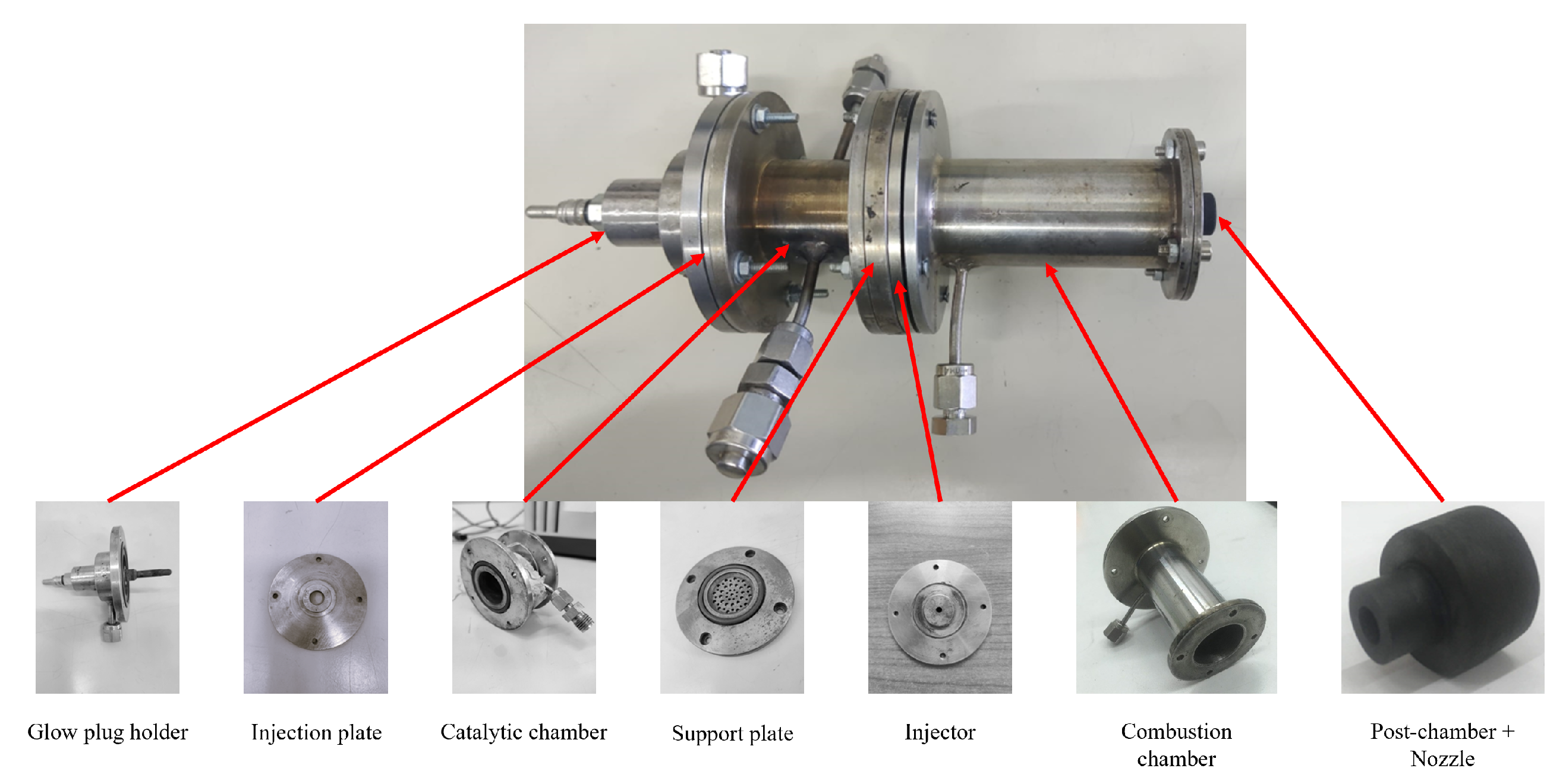
As mentioned, the thruster has already been tested for different fuels in previous works. The assembled thruster and individual components that make it up are shown in Figure 2 [9]. As can be seen, it is equipped with a number of sensor sockets for the acquisition of temperature and pressure readings during the test. In this case, our attention is focused on the thrust chamber, represented by the last steel block in the figure. The oxidant is injected through aconical injector with a diameter of 2 mm, then enters the combustion chamber, which houses a fuel grain 40 mm in length with an initial diameter of 10 mm. This combustion chamber features a pre-chamber that is 15 mm long and has a diameter of 21 mm. Downstream of the fuel and in direct contact with it is a single graphite body that forms both the after-chamber and the nozzle, as shown in the Figure 2. The after-chamber is 10 mm long with a diameter of 16 mm. The nozzle has a throat diameter of 2.1 mm and a relatively low expansion ratio of 1.49, as the tests are carried out at ambient pressure.
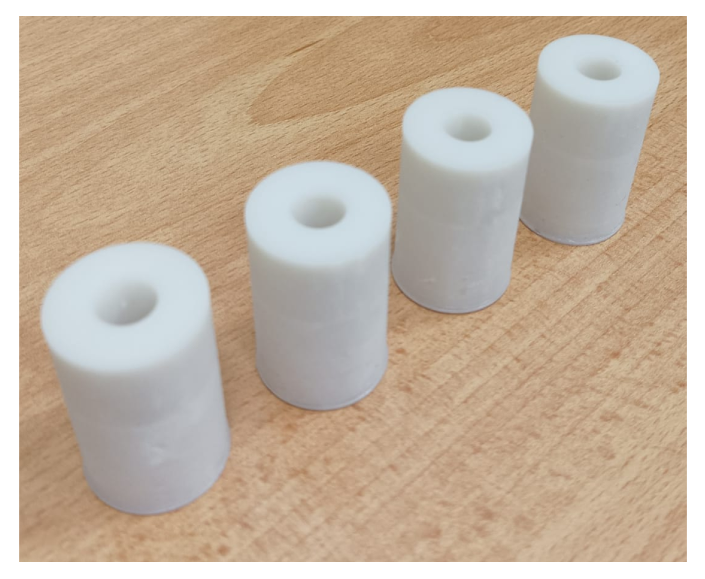
With regard to propellants, commercially available 60 wt% hydrogen peroxide was distilled with the aim of reaching a highly concentrated solution of hydrogen peroxide (concentration of 87.5 wt%) for use as the oxidizer. The decomposition is catalytic, using MnOx-based catalysts contained in the catalytic chamber, as reported in Figure 2. The catalysts ensure high efficiency and very short response times (on the order of tenths of a second) compared to other catalysts such as Palladium [15]. The fuel is a solid 3D-printed ABS cylindrical grain obtained from a commercial resin by the AnyCubic Company (www.anycubic.com (accessed on 21 January 2025)), and has a density of approximately 1200 kg/m3. Figure 3 shows an example of some 3D-printed cylindrical grains.

3. Postprocessing and Data Reduction Techniques

3.1. Data Analysis Methods and Errors

In addition to temporal analysis of the measurements, the mean values of the most relevant quantities were derived from the measured data. The main parameters directly measured in the firing tests were the oxidizer mass flow rate m ˙ o x , chamber pressure p c , motor thrust F, fuel grain mass consumption Δ M , and the burning time t b . With regard to the derived quantities, the formulas below were used to obtain the main parameters [10].
The average oxidizer mass flux can be calculated as follows:
G ¯ o x = 4 m ˙ o x π D ¯ p 2
where D ¯ p is the time–space-averaged port diameter. The mean fuel regression rate over time and space can be calculated as follows:
r ˙ ¯ = D ~ p , f i n D p , i n 2 t b
where D ~ p , f i n and D p , i n are the initial and space-averaged final port diameters. In particular, when the space-averaged final port diameter is calculated as an average of the inlet and outlet diameters measured with the caliper, it is referred to as a measurement acquired with the “caliper”. However, when the diameter is calculated based on the mass lost by the fuel using D p , i n 2 + 4 Δ M π ρ f L , it is referred to as the “mass loss method”. Finally, the time-averaged experimental characteristic velocity is calculated in the following way:
c = p c A t m ˙ t o t .
The primary sources of uncertainty associated with the measured quantities are:
  • The burning duration, i.e., the time interval between the inflection point on the pressure rise branch at motor start-up and that on the pressure drop at the burnout.
  • The diameter measurements for the grain port that exhibit dispersion.
  • The scale sensitivity for the initial and final grain mass measurements.
  • The signal oscillation during the oxidizer mass flow rate measurement.
The associated errors for the instrumentation are presented as follows:
  • Thermocouple accuracy: ±5 K.
  • Pressure transducer accuracy: ±0.7 × 10 4 Pa.
  • Load cell accuracy: ±0.05 N.

3.2. Ballistic Reconstruction Technique

This numerical procedure enables reconstruction of the regression rate over time during the test. While a single test provides a single regression rate value for a given mass flow ( G o x r ˙ ), the ballistic reconstruction technique allows for the derivation of multiple regression rate points, from which a regression law can then be derived.
Reconstruction techniques include various approaches [16,17,18]. In this work we employ the simplified method, which does not rely on a detailed thermochemical database for the selected fuel, as a thermochemical database for the studied 3D printed ABS does not yet exist.
However, as has already been demonstrated, the most simplified technique which does not require thrust measurement still allows for very reliable solutions [19].
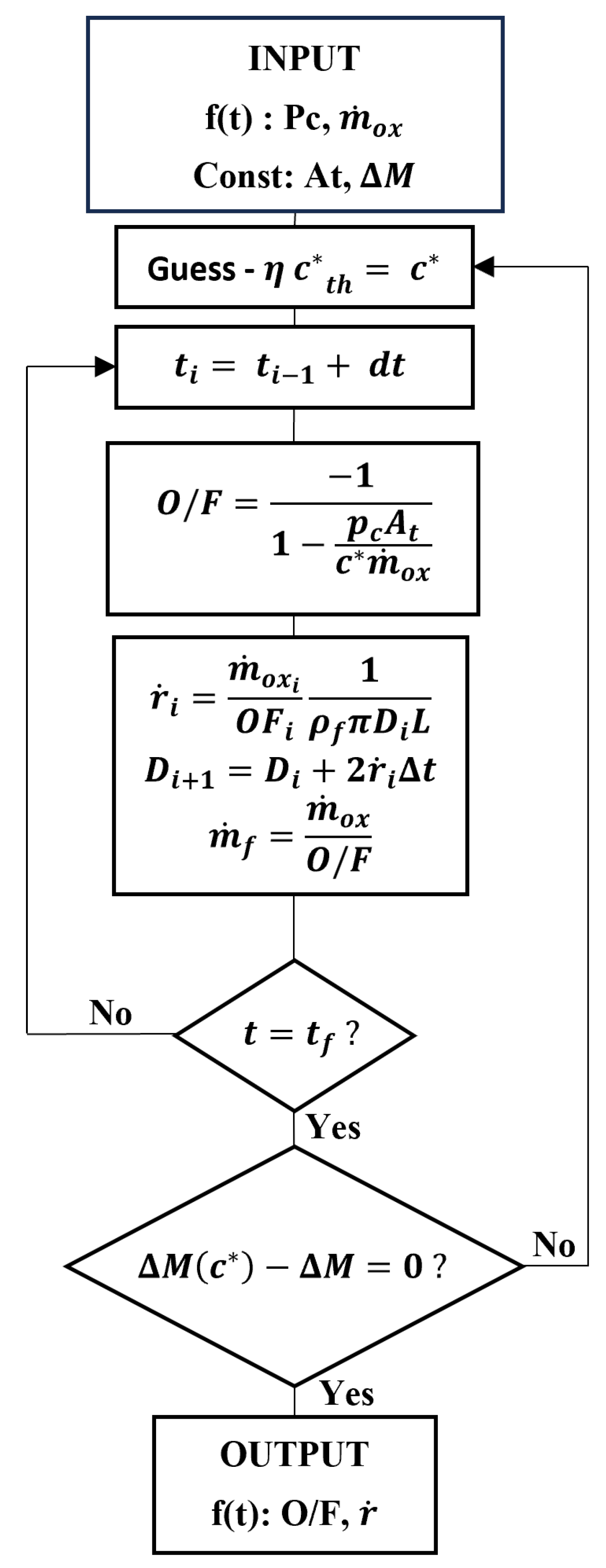
The diagram in Figure 4 shows the logical flow underlying the ballistic reconstruction technique. The input parameters for the simplified procedure are the chamber pressure, mass flow rate, Δ M , nozzle throat area, and product of efficiency η with the theoretical characteristic velocity c t h . Here, efficiency is defined as the ratio between the experimental and theoretical characteristic velocities; this product represents the time-averaged experimental characteristic velocity c reported for each test in Section 5. In general, the method involves calculating c t h using the Chemical Equilibrium Applications (CEA) software (https://cearun.grc.nasa.gov (accessed on 21 January 2025)) [20], and the efficiency is varied until convergence is achieved. In this case, because the properties of the fuel are unknown and are likely differ from those reported in the literature for ABS [11], c is directly used as reference value. The equation for determining O / F i at the i-th time step from, which the space-averaged regression rate r ˙ i is computed, is the mass balance equation, which is reported in Equation (4). Finally, the procedure converges when the difference between the mass lost by the fuel in the simulation Δ M ( c ) and that lost experimentally ( Δ M ) becomes sufficiently small to be acceptable. In this case, we decided that the difference between these two values should be less than 10% of the mass loss of the fuel in the experiment:
1 + O / F O / F p c A t c m ˙ o x = 0 .

3.3. Performance Calculation Procedure

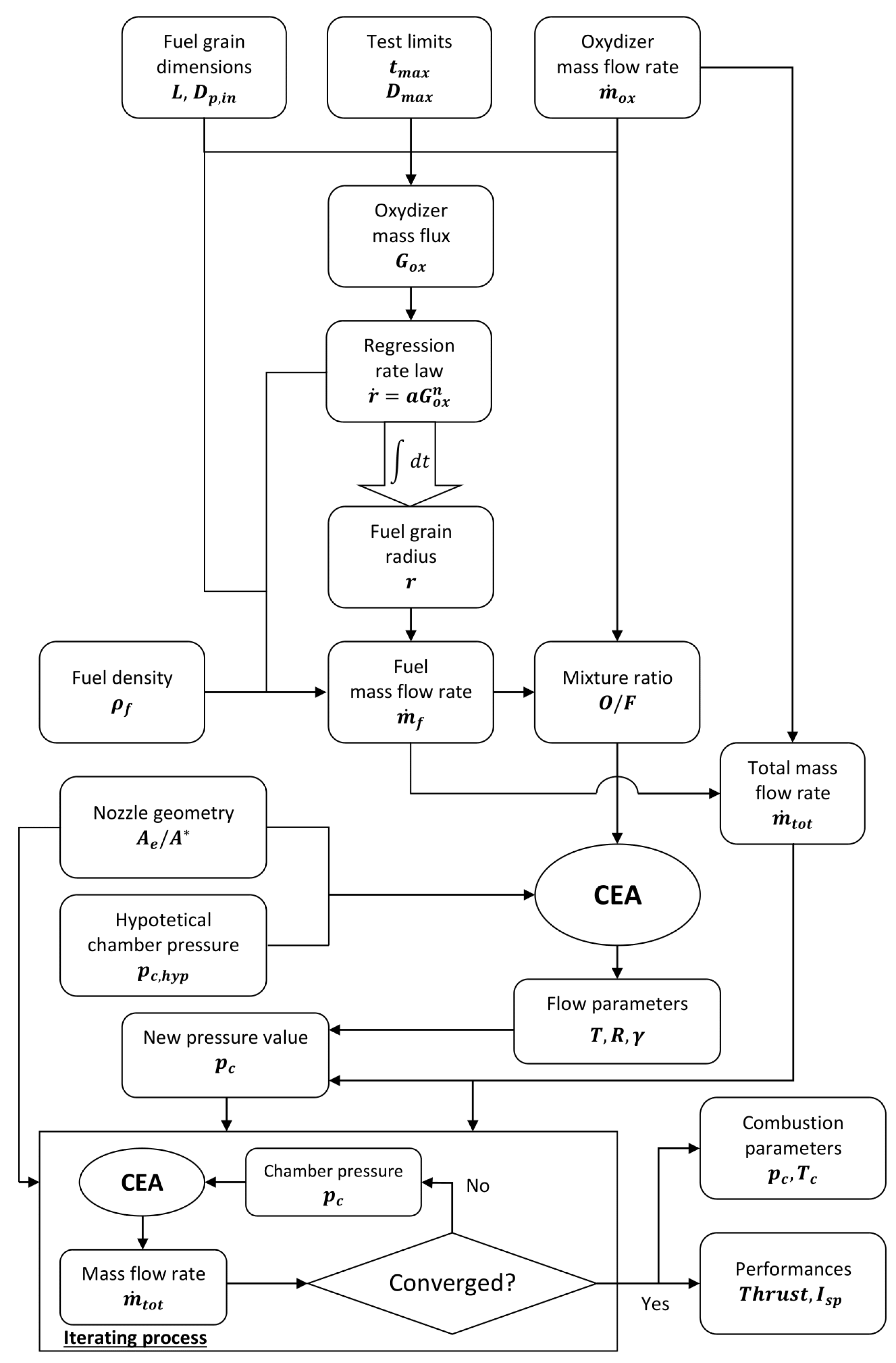
In order to verify the validity of the regression laws obtained in this work, a Matlab code was used to estimate the performance of a hybrid propellant rocket, providing a known regression law as input from among various parameters. In this case, both the regression rate derived from ballistic reconstruction and that obtained from the average experimental values from the tests are used as input. Specifically, using the regression laws found as input, we verified that the main propulsion parameters resulting from the simulation match the experimental ones within a small percentage error. Figure 5 shows the workflow behind these numerical simulations; as indicated, this procedure also uses some outputs provided by NASA’s CEA software (https://cearun.grc.nasa.gov (accessed on 21 January 2025))and is described by [21].

4. Computational Model

4.1. Numerical Model and Boundary Conditions

In this section the physical model for the CFD simulation of the thermo-fluid dynamic flowfield in the combustion chamber and through the nozzle of the hybrid rocket is presented in order to derive the parameters characterizing the pyrolysis of the 3D printed ABS based on the results obtained experimentally. The simulations were performed using the commercial software Ansys FLUENT (https://www.ansys.com/products (accessed on 21 January 2025)).

4.1.1. Numerical Model

The governing equations underlying the numerical model are provided in detail in Appendix A, while a summary is provided below. Primarily, a model of RANS equations for a single-phase multi-component turbulent reactant flows is employed, which is solved with a technique for control volumes and a pressure-based algorithm.
  • The selected turbulence model is the SST κ ω , due its superior ability to adequately capture the phenomena that occur in the near-wall region in comparison to other models. For the purposes of this study, such as for calculating the fuel grain regression rate and examining phenomena near the grain wall, it is the most suitable model [22].
  • The combustion model is non-premixed between the oxidizer and the fuel injected from the grain surface. Considering the monomer C4H6 as a product of pyrolysis, it is assumed that the reactions are much faster than the rate at which the species diffuse into the engine. Thus, the model is formulated with a chemical equilibrium-based Probability Density Function (PDF) approach, with the entirety of the system being reduced to a single transport equation for the mean mixture fraction f = 1/(1 + O / F ), where O / F is the local oxidizer-to-fuel ratio of the equivalent non-burning field. Chemical–turbulence interaction is considered, closing the model with the variance equation of f [23].
  • The thermodynamic and transport properties are derived from the solver chemical database. In particular, thermal conductivities and molecular dynamic viscosities are computed as a function of local temperature, with coefficients obtained from [20].
  • Finally, it is necessary to describe the interface in the model between the gas phase and the fuel surface in order to describe the mechanism by which the fuel is consumed. Therefore, the following two equations are considered under the assumptions that no matter is removed from the condensed phase surface. In addition, convective and diffusive heat transfer in the energy balance equation are considered, while the radiative part is neglected:
    ( ρ v ) w = ρ f r ˙
    q w = ( λ g T n ) w = ρ f r ˙ [ Δ h p + C f ( T w T i n ) ]
    where ρ is the gas density at the wall, v is the normal-to-wall velocity component due to injection of the pyrolysis products, ρ f is the solid fuel density, r ˙ is the local regression rate, n is the normal-to-surface oriented from solid to gas, λ g is the thermal conductivity of the gas, C f is the solid heat capacity per unit mass, Δ h p is the heat of pyrolysis, T w is the fuel surface temperature, and T i n is the initial temperature.
  • Pyrolysis of the fuel is described by the semi-empirical Arrhenius-type equation, as in [24]:
    r ˙ = A e ( E a 2 R T w )
    where A is the pre-exponential factor, E a is the activation energy, and R is the universal gas constant. The following paragraphs discuss the determination of the Arrhenius coefficients in detail.
  • Transient simulations were conducted to address model limitations, including the neglect of non-uniform regression rates and inner grain diameters. In the stationary simulation, the regression rate was averaged and uniform along the grain length, and the same was true for the inner diameter. Consequently, a series of simulations was performed in which the local diameter of the port was updated at each instant based on the local regression rate calculated at the previous instant [25].
In particular, the fluid–solid interface boundary undergoes changes over time in the context of surface regression. The displacements of the computational grid nodes are not uniform throughout the grain length, according to the local regression rate calculated from Equation (7); moreover, as the regression rate is defined in the direction normal to the fuel surface, displacement of a generic point occurs. In the present study, forward numerical integration of the local fuel regression rate is implemented for the purpose of calculating the displacement of the grid nodes. The process begins with a specific grain port profile at the n-th time step, which is defined by the vectors of the axial and radial coordinates x i n y i n of the grid nodes (here, the subscript i indicates the i-th node). A CFD simulation is carried out using the aforementioned model to compute the fuel regression rate distribution r ˙ n ( x i ) at the designated time step n and axial location x i . The regression rate is then integrated forward to determine the displacement after a fixed temporal increment Δ t .
After the new distribution is calculated, the fluid domain geometry is modified by using the Ansys ICEM software (https://www.ansys.com/products (accessed on 21 January 2025)), the computational mesh is adjusted to the new geometry, and a new numerical simulation is performed at the new time step.

4.1.2. Boundary Conditions

Concerning the boundary conditions, no-slip and adiabatic boundary conditions are imposed on the inner surface of both the pre-chamber and post-chamber as well as on the nozzle wall. At the injector section, a mass flow boundary condition is prescribed along with the temperature and mass fractions of hydrogen peroxide decomposition calculated using chemical equilibrium analysis. In particular, the mass fractions of oxygen and water vapor are obtained using NASA’s CEA code, and depend on the HTP concentration, which in this case is 87.5%. The gas temperature at the injector is defined based on the experimentally derived decomposition efficiency; this efficiency indicates the percentage of liquid hydrogen peroxide that is completely decomposed in the catalytic chamber, which is obtained through an iterative procedure using the CEA code. Specifically, the concentration of decomposed peroxide is imposed as a guess, then the corresponding CEA results allow obtaining the parameters (density and specific heat ratio) needed to calculate the oxidizer flow rate by means of Bernoulli’s formula for subsonic compressible flows, as the oxidizer is injected in the gaseous state due to the decomposition process in the catalytic chamber and the injector is not choked because the pressure ratio between the combustion chamber and the catalytic chamber is higher than the critical value. The iterative procedure stops when the efficiency value allows the calculated flow rate to be matched with the experimentally measured one [19]. For the experiments in this work, the efficiency is about 90%, which results in a gas temperature of approximately 900 K (from the CEA simulations); this value is used as a boundary condition for the injector. Finally, a pressure outlet condition is set at the nozzle exit section.
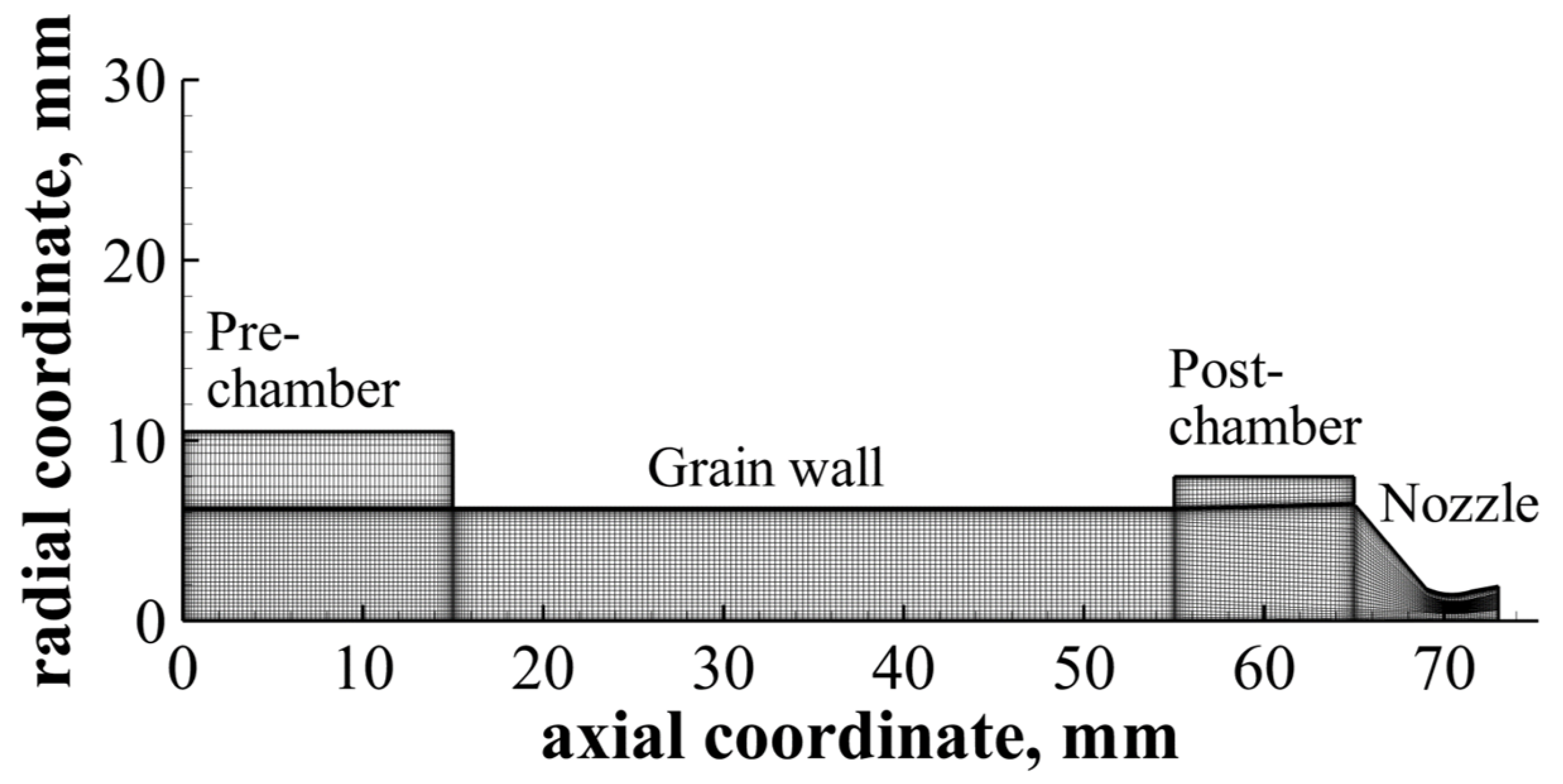
Figure 6 shows a typical mesh used for the hybrid rocket thrust chamber. Note that this is only an example, as the grain port diameter changes for the different cases under consideration. As seen from Figure 6, the cells are clustered towards the grain wall, meaning that the maximum y + is around 1 at the adjacent cell along the grain length for all considered test cases. The main dimensions are listed in Table 1.

4.2. Grid Sensitivity

A grid sensitivity analysis was performed in order to ascertain the spatial dependence of the numerical results. The analytical procedure followed Richardson extrapolation [26], with the Grid Convergence Index (GCI) derived using the following equations:
G C I f i n e = F s | f r e f f f i n e f f i n e | r z 1 ,
G C I c o a r s e = F s | f r e f f c o a r s e f r e f | r z 1 ,
where r = 2. This value was chosen because the fine and the coarse meshes were obtained by doubling and dividing the number of nodes by 2, starting from the reference mesh; z is the order of accuracy, which is obtained with the following equation:
z = l n ( f c o a r s e f r e f f r e f f f i n e ) l n ( r ) .
where F s is a safety factor equal to 1.25 used for comparison of the three meshes [26].
As demonstrated in Table 2, the results indicate that both GCIs are small, meaning that the numerical solution tends to be asymptotic. This is demonstrated by the following relationship [27]:
G C I c o a r s e r z G C I f i n e .
From the above, it can be deduced that the resulting errors will be negligible for any mesh. Consequently, we employed the reference grid in our study of the internal ballistics of the experimental tests, as it provides a fair compromise between solution accuracy and computational load.

4.3. Determination of the Arrhenius Coefficients

As explained above, the calculation of the regression rate in Section 4.1.1 relies on the physical parameters of the fuel, which appear in Equations (6) and (7). Unfortunately, data on the pyrolysis properties of ABS are limited in the scientific literature, and are also strongly dependent on the specific production process. In addition to affecting chemical parameters such as density, these properties also play a crucial role in determining mechanical properties such as roughness; for example, filament printing generally results in a rougher surface compared to fused deposition printing.
Work by Whitmore [11] and Wilson [28] has identified systematic approaches for the characterization of two types of ABS obtained by two different processes. These works identified extruded ABS and rapid-prototyped ABS obtained via the Fused-Deposition Modeling (FDM) technique. The properties of these ABS formulations are reported in Table 3. It can be observed that the main differences between the two formulations are in the pre-exponential factor A and the activation energy E a .
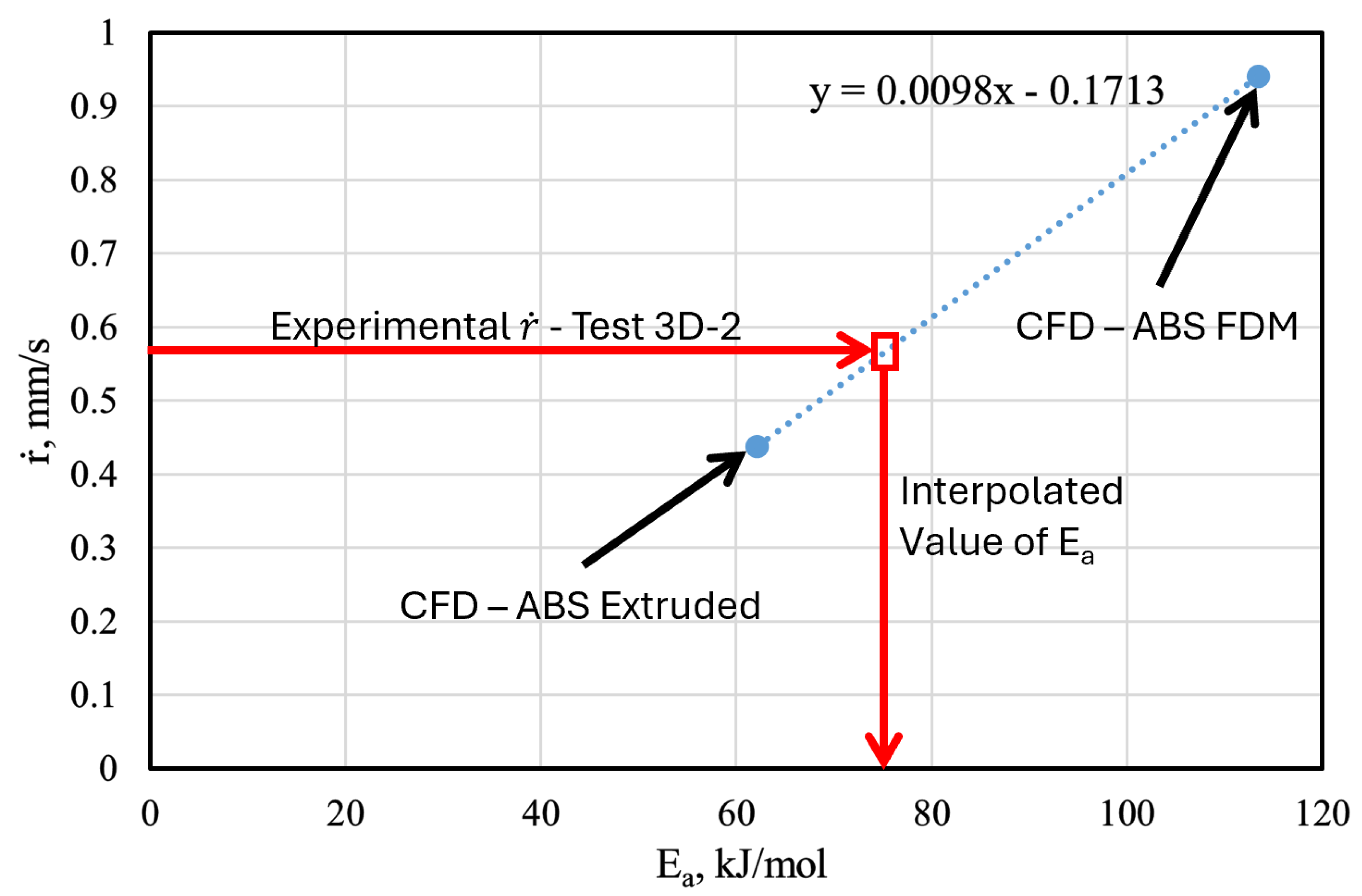
In order to determine the values of these two parameters for use in modeling the 3D-printed ABS used in our tests, we adopted the following procedure. First, CFD simulations were carried out in the average experimental conditions of one of the present tests (3D-2; see Section 5.1) using the Arrhenius parameters of the extruded and FDM ABS from Table 3. The obtained values of the regression rates are plotted in Figure 7 and Figure 8 versus E a and l n ( A ) , respectively. Then, as a simplifying hypothesis, it was assumed that the regression rate depends bilinearly on these two parameters. Based on the obtained linear interpolation functions, the values of E a and A corresponding to the experimental regression rate of the reference case were found. The procedure is illustrated by the red arrows in the Figures. The parameters obtained in this way were then used for all simulations; as we show later in this paper, they provide very reliable results.
The results show that rate constants of 3D-printed ABS are closer to extruded ABS, as evidenced by Figure 9, in which the regression rate trends from Arrhenius’ law are plotted against the inverse of the average grain wall temperature on a log-scale graph.
Because the pyrolysis heat values are about the same, no further interpolation was necessary for the other data. For the density, a value of about 1200 kg/m3 was used, as mentioned above. Table 4 summarizes the properties for our 3D-printed ABS simulations.

5. Results and Discussion

This chapter discusses all of the obtained results, both experimental and numerical. We first present a performance analysis, after which we characterize the regression rate in dependence on the mass flux by means of ballistic reconstructions and analyze the local distribution of the grain consumption. Finally, by means of both stationary and quasi-stationary numerical simulations, we show how the numerical model using the aforementioned Arrhenius parameters turns out to be very reliable in terms of both average magnitudes and the local distribution of the fuel consumption, with the errors always falling below the 10% level.

5.1. Test Matrix

Table 5 shows the operating conditions and thruster configuration of the three tests carried out in the Propulsion Laboratory. Tests were performed at different mass flow rates, with the objective of characterizing the regression rate of ABS using hydrogen peroxide as an oxidant. All tests were pressure-regulated, and the fuel was ignited after a sequence of five pulses in order to preheat the system and reduce the ignition delay. Using a sequence of five pulses allows the catalytic system to be heated; at the same time, the hot gas generated by the decomposition enters the combustion chamber and raises the temperature of the fuel, which begins to pyrolyze. Therefore, catalytic-type ignition occurs when switching the flow to continuous mode. This in turn causes the amount of pyrolyzed fuel to increase to the point where a mixing ratio with the oxidizer is achieved, which is sufficient for ignition of the flame.

5.2. On-Ground Performance

Table 6 shows the experimental results obtained as explained in Section 3.1. The burning time is considered as the time from half-rise to half-fall of the pressure history. An example showing representative curves of the measurements is provided in Figure 10. The blue curve represents the pressure in the catalytic chamber, the yellow curve the pressure in the combustion chamber, and the green curve is the thrust. A delay of approximately half a second can be observed before reaching the steady state, where relatively constant values indicate smooth combustion. These considerations can be repeated for all the experimental cases.
Looking at the time histories in detail, a slight decrease in pressure in the combustion chamber can be seen for the different tests. Because the thrust also shows the same trend, and as no erosion of the graphite nozzle was observed, this phenomenology can be explained by the reduction in total mass flow rate. The oxidant flow rate during the test is almost constant, indicating a slight reduction in fuel flow rate as the grain widens. This is shown below, and can be verified by ballistic reconstructions of the tests and the regression law in dependence on the mass flux.
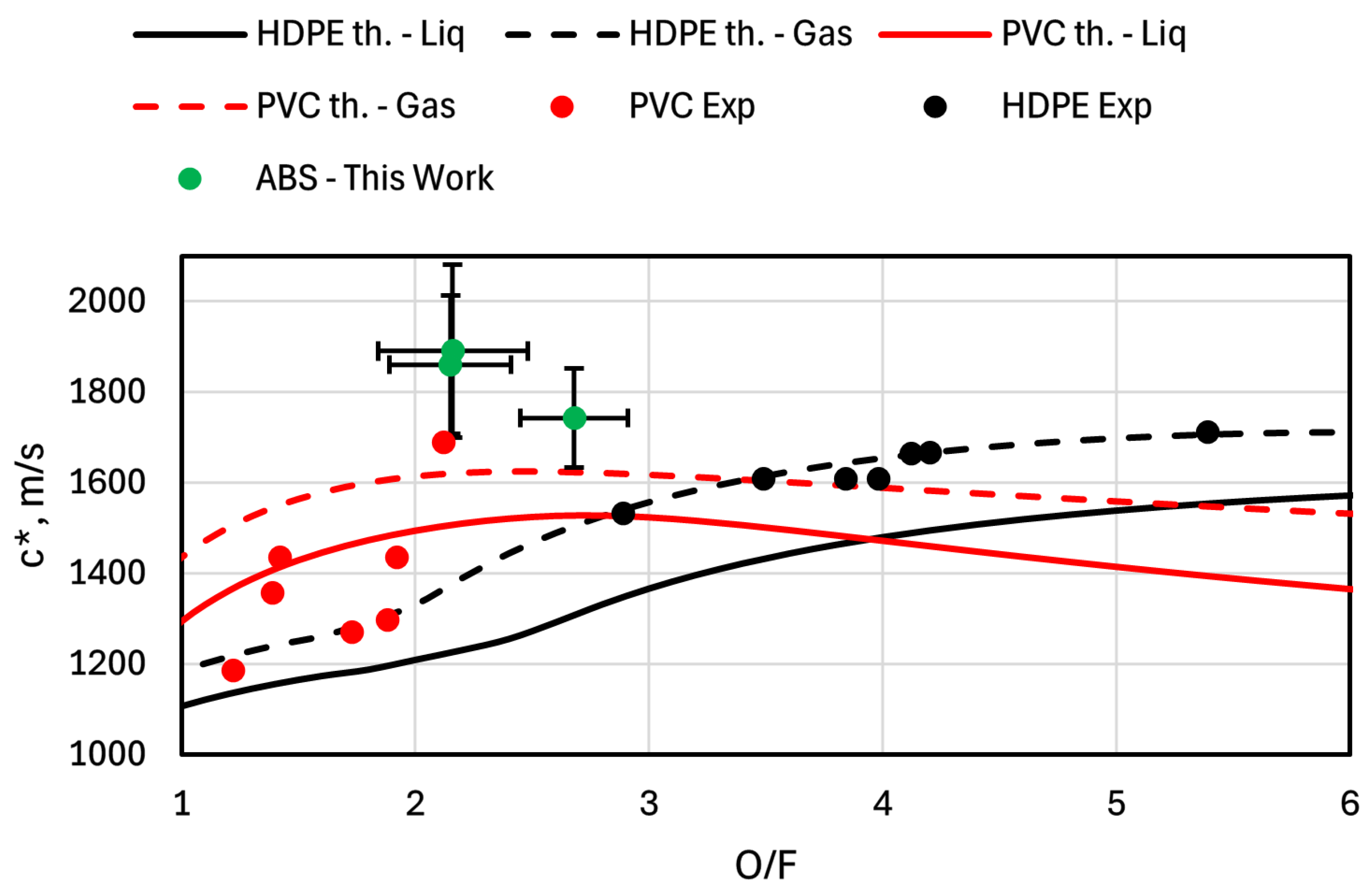
In Figure 11, the experimental characteristic velocity values of the current tests are compared with experimental ones from previous campaigns in which the fuels under study were PVC and HDPE [29]. For the two aforementioned fuels, theoretical curves are also provided for the cases of fully gaseous and liquid injections of hydrogen peroxide. For 3D-printed ABS, no thermodynamic database is available for accurately calculating the theoretical characteristic velocity curves with respect to O / F . However, although it is not possible to provide an accurate assessment of the combustion efficiency, it is still possible to discuss the comparison of experimental characteristic velocities in the case of tests using these three different fuels per fixed oxidant. It is notable that the hydrogen peroxide–ABS pairing obtains greater c compared to PVC and HDPE. It is possible that the theoretical curves of this material are higher, which could be very useful in the context of CubeSat space missions by ensuring propellant savings due to the higher specific impulse.

5.3. Reconstruction Technique Findings

Figure 12 illustrates the observed trend in the mixing ratio. For each of the three tests presented and reconstructed in Section 5.2, we obtained the O / F trend over time. Each point refers to the instantaneous value of O / F . The sampling time was set to 0.1 s. In Figure 12, all the points obtained from each test are shown together, as the goal in this case is to demonstrate the mixing range in which the three tests were conducted. As can be seen, the O / F in the various tests is in the range of 2 to 3. For each test, the particular O / F ratio is slightly increasing, meaning that the fuel flow rate during the test decreases slightly, as mentioned earlier in the analysis of pressure history from Figure 10.
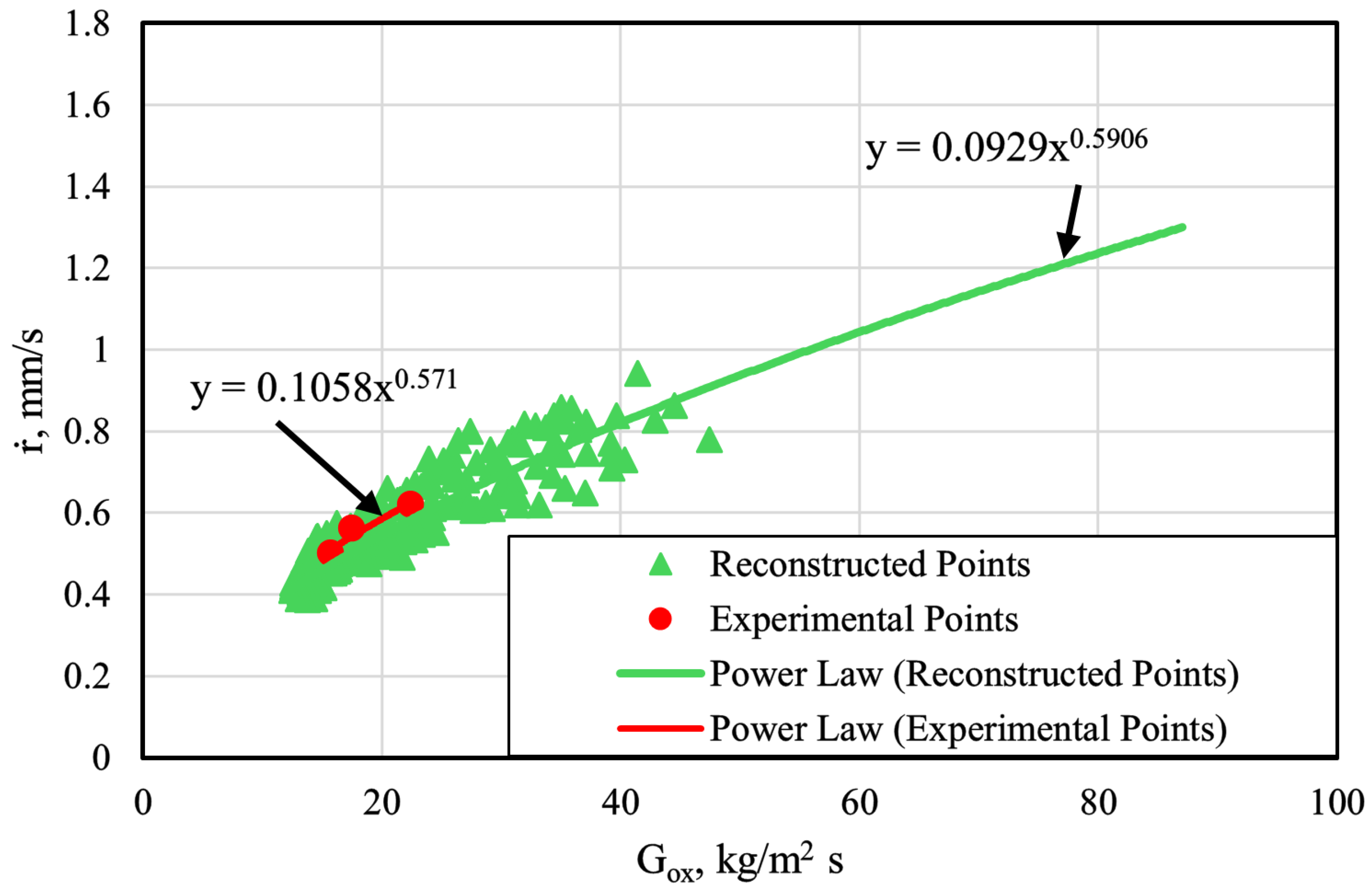
Figure 13 displays the power law derived from the experimental data along with the one derived from the ballistic reconstruction data. The green curve represents the interpolation of the green data points, which were obtained through ballistic reconstruction of all tests and plotted using the same principle as in Figure 12. The G o x at each point represents the instantaneous mass flux based on the instantaneous values of oxidizer flow rate and port diameter. On the other hand, the red curve is derived from interpolation of the red data points, which are obtained from experiments calculating time–space-averaged mass flux and regression rates from Equations (1) and (2), respectively. The distinction between the two curves can be discerned by noting that they have been slightly translated with respect to one another. In fact, the slopes of the two curves are comparable.
It is important to emphasize is that the regression curve written in the form of the Marxman law [30] shows an exponent greater than 0.5 in both cases. This relates to what was mentioned earlier, namely, that with the reduction in mass flux of the oxidizer due to the increase in the port diameter, the regression rate decreases quite steeply, which reduces the overall fuel flow despite the increase in the pyrolyzing surface.
Furthermore, we employed a a Matlab code, the workflow of which is presented in Section 3.3, to verify the validity of both laws. As evidenced in the accompanying Table 7 and Table 8, the discrepancy between the calculated numerical values and the observed average values obtained from the experimental measurements is minimal.
The two power laws yield results that are comparable to each other. Although a regression law obtained through experiments would be more significant, it is preferable to consider the law obtained from ballistic reconstruction for the purpose of characterizing the material. This is because the proposed technique reproduces experimental cases with minimal errors and generates a substantial number of points over a wide range of mass fluxes.

5.4. Local Distribution of the Fuel Consumption

After completing the tests, we conducted a detailed analysis of the axial distribution of the grain port diameter profile. The methodology behind this technique is outlined in [31]. After the fuel grains have been extracted from the engine, a longitudinal incision on the grain is made using an electric hacksaw to yield a half-cylinder fuel grain, as illustrated in Figure 14.
The arrow indicates the flow direction of the engine from upstream to downstream. The cylinder was divided into eight equal sections with a distance of 5 mm. The inner diameter of the fuel grain was measured using a caliper gauge. To ensure the most accurate result, four measurements were taken for each section. From these, the minimum, maximum, and average diameter of the section were taken into account.
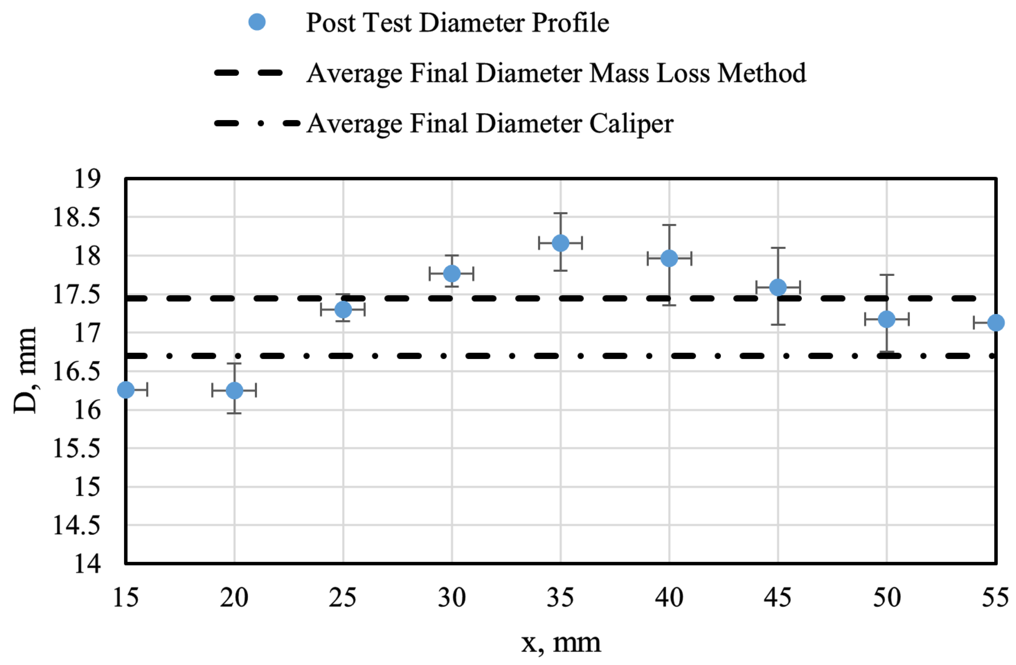
Figure 15 shows the longitudinal distribution of the inner diameter of the grain for Test 3D-2, including the average values obtained by the mass loss technique and the caliper. The error bars were calculated using the minimum and maximum values of the measurements. It can be seen that the mean mass loss value is close to the distribution along the axis. As expected, the mean caliper value moves away from the values in the center of the grain and is close to the outer values, as the measurement with the caliper is based on the measurements taken at the inlet and outlet of the grain. The same applies for all other experimental tests.
This approach allows the numerical model to be validated through both steady and transient simulations, starting with the initial grain port diameter, then performing measurements before the experiment and evolving the result in time steps, as explained in Section 4.1.1. In this way, the distribution of the port diameter can be obtained and compared with the experimental results obtained with the slicing technique.

5.5. Fuel Characterization via CFD Simulations

After performing the experiments, the CFD models and techniques described in Section 4.1.1 were used for more detailed characterization of the fuel behavior, especially in terms of the regression rate. As explained above, detailed thermo-chemical properties are lacking; therefore, a combined numerical and experimental approach was considered in order to derive some of the fuel parameters, which are relevant for future thruster design developments. The main outcome of the simulations presented below is the regression rate profile, which can be compared with experimental measurements. In addition, we present the structure of the flow field in terms of static temperature and flow pathlines, as these directly affect the heat transfer to the solid fuel surface and consequently impact the regression rate.

5.5.1. Steady-State Simulation

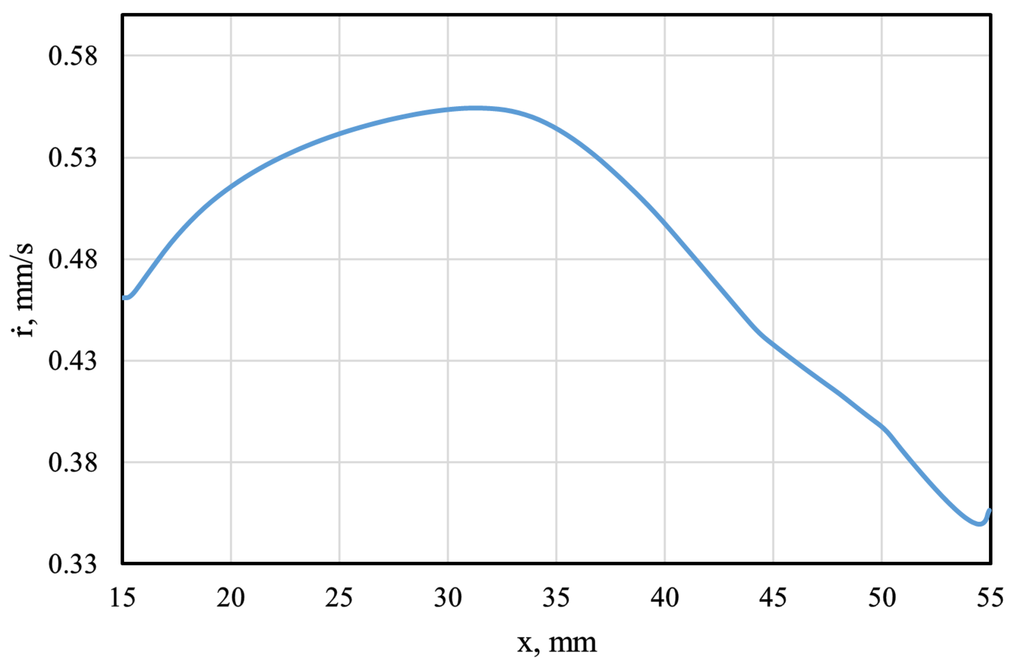
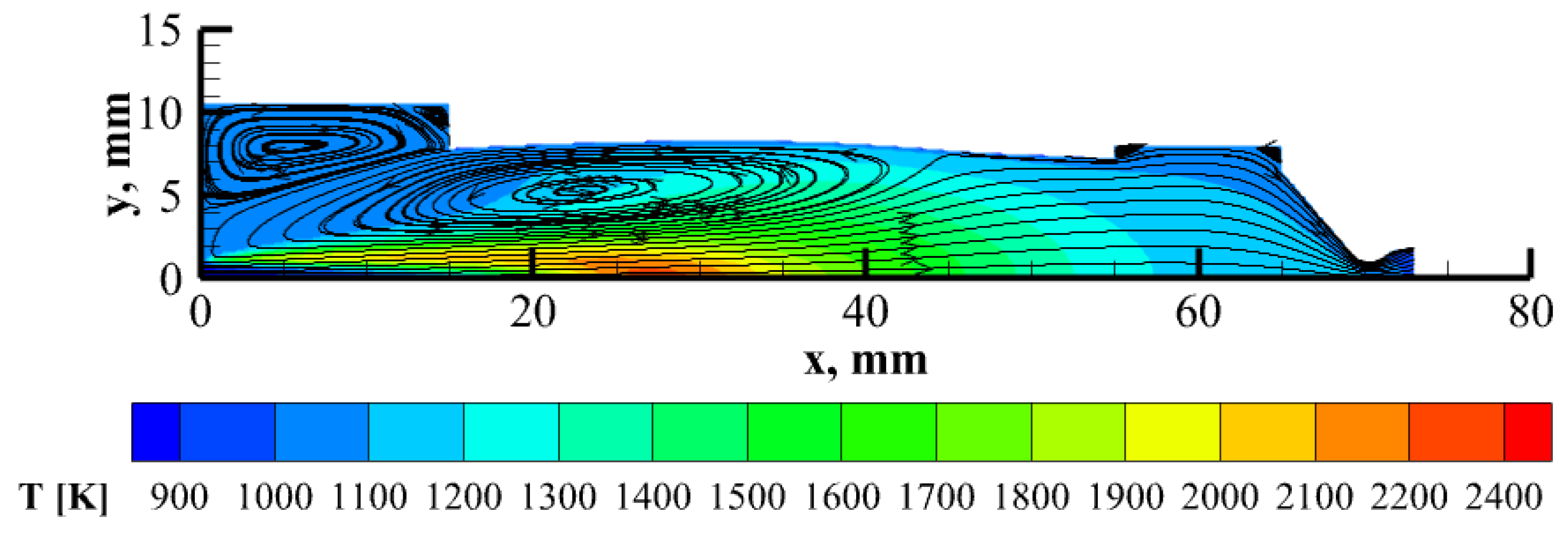
The objective of our stationary CFD simulations was to replicate the experimental tests as accurately as possible. In general, the inputs that differ among the tests were the oxidant mass flow rate, time–space-averaged port diameter, and temperature of the injected oxidant. These values were derived from the experiments; specifically, the flow rate and port diameter for each test are shown in Table 6, while the gas temperature was approximately 900 K for all tests, as explained in Section 4.1.2, since the decomposition efficiency was always about 90%. To illustrate this, the simulation of experimental test 3D-1 is presented as an example; however, the following considerations can be applied to all tests under examination, the results of which are reported in the Supplementary File. Figure 16 depicts the static temperature contour and the pathline trajectories within the thrust chamber; specifically, Figure 17 shows the regression rate trend along the axial direction resulting from the numerical simulation. It is evident that a very extended recirculation zone is present, with reattachment corresponding to the curve maximum in Figure 17 at approximately the midpoint along the grain. Indeed, the flow field and flame distributions are quite unusual compared to what is reported in the current literature. The reason for this is primarily that in this case the axial injector diameter is much smaller than the port diameter, resulting in a very large recirculation zone before it reattaches to the fuel wall. This leads to a very large area in which the mixture is fuel-rich, with the flame layer being confined near the engine axis and distant from the fuel wall (see Figure 16).
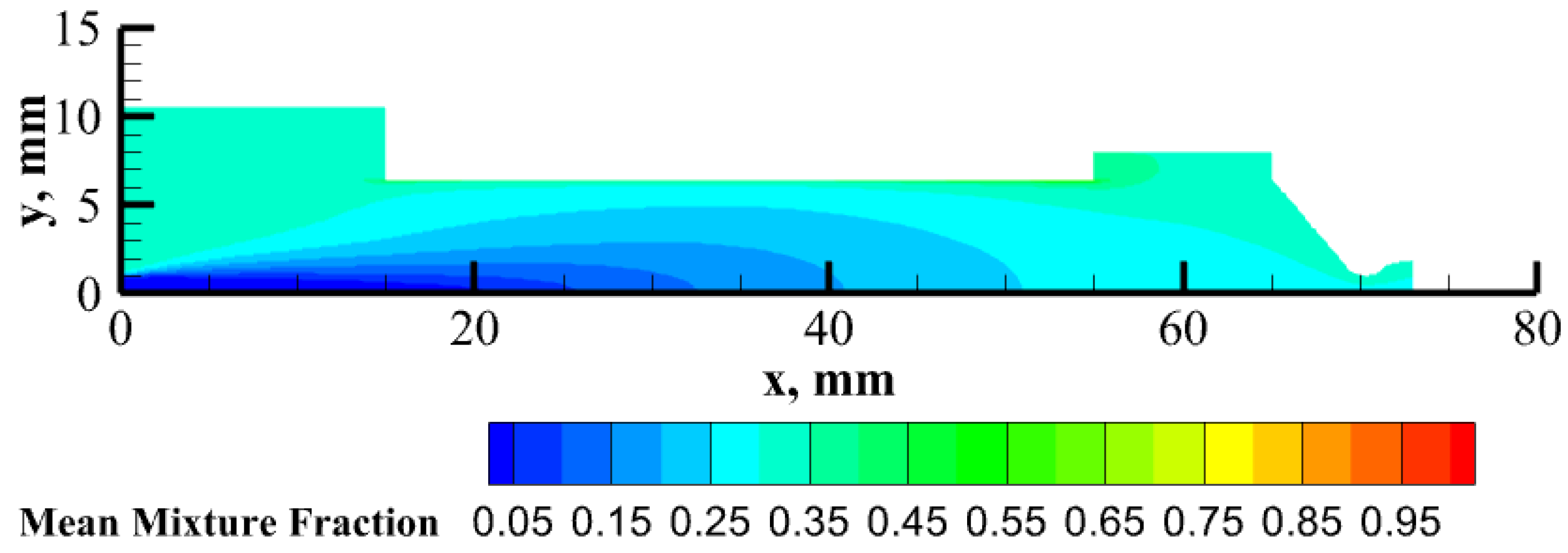
Another relevant aspect to note from Figure 16 is that the mixing in the post-chamber is rather poor compared to what is usually expected [32], resulting in the presence of a relatively cold zone. Additionally, a flame is observed to be confined in the axial direction up to about halfway through the fuel. These phenomena are mainly related to the fact that the oxidizer mass flux is very low, even an order of magnitude lower than the works present in the literature [33]. This causes the flame to “close” early in the axial direction, as most of the oxidizer entering the chamber is burned in that zone, leaving space for a fuel-rich zone. To support this hypothesis, Figure 18 shows the contours of the f-function (defined in Section 4.1.1), which for the propellants used here is 0.13 in the case of stoichiometric mixing. Where it is greater than 0.13, the zone is fuel-rich, and there are points where the temperature is just over 1000 K, in agreement with what is reported by NASA’s CEA software. In contrast, at higher mass fluxes the amount of oxidizer required to achieve a stoichiometric mixture is still available in regions far from the injector, and a flame zone is observed, in some cases all the way to the nozzle [34].
Table 9 presents the average regression rates and average wall temperatures for all numerical simulations of the experimental cases. The fact that the percentage error obtained in the case of test 3D-2 is not zero, and is actually the highest, indicates that the regression rate does not have perfectly bilinear dependence on the activation energy and natural logarithm of the pre-exponential factor. In any case, the relative error between the experimental test cases and the numerical ones is below 10%, providing evidence in support of the numerical model’s reliability. Because the Arrhenius law was derived from an experimental test, this is observed to be an effective modeling approach for simulating tests with different oxidant mass fluxes, as the methodology for selecting the parameters is independent of the mass flux. This ensures a reliable model for studying the internal ballistics, and consequently supports the design of engines fueled by ABS-based 3D-printed fuels.

5.5.2. Transient Simulation

As the diameter of the fuel grain port expands over time, the recirculation zone also undergoes a shift in position relative to what is observed in the stationary case through both the pathline trajectories and the regression rate trend. To evidence this shift and obtain the most accurate results in terms of the local distributions of the port radius and regression rate, we performed transient simulations. Here, “transient” refers to a series of steady-state simulations that are anticipated to differ from each other through the local distribution of the port diameter. In fact, because the chemical and fluid dynamic characteristic times are much shorter than the regression velocity timescale, the evolution of the geometry over time can be simulated with a series of steady-state simulations [35].
The static temperature contours and pathlines from the transient simulations are displayed in Figure 19 and Figure 20, respectively corresponding to the initial time step and to one second prior to termination of the test. Here, the 3D-2 test was the subject under consideration, and the intermediate steps are reported in the Supplementary File). It was decided to advance the distribution of grain port diameters in increments of 1 s; thus, the final port diameter distribution was obtained from the regression rate and the port diameter distributions in the simulation performed at t = 6 s. As depicted in the figures, at t = 0 s the recirculation zone is confined between the pre-chamber and the entrance of the combustion chamber. At the final time step, the evolution of the recirculation zone is noteworthy in that it moves towards and beyond the central part of the grain, resulting in non-uniformity of the grain wall along the axial direction with respect to the well-known larger-scale thrusters. The recirculation area is very large in this case, as previously reported, and is not limited to the zone between the pre-chamber and the initial part of the grain.
Figure 21 compares the results obtained using the previously-described slicing method with the results of the transient simulations. It can be seen that the axial positions of the numerical and experimental maximum values match quite well and are positioned at approximately the halfway point of the grain. In summary, the trend of the wall regression profile exhibits notable alignment between the experimental and numerical cases at the final time step. The only more evident difference is visible at the fuel outlet, where the experimental measurement is higher than the numerical result, although the error is still below 10%. As will be seen shortly, this leads to overall average values with an error smaller than 10% compared to the experiment. This discrepancy is probably related to possibility of the grain undergoing greater overheating in the post-chamber area due to the high thermal fluxes that heat the graphite post-chamber. This could lead to an increased regression rate, which the model is unable to capture in this case because the fuel is set to an initial temperature of 300 K. However, modifying the model to investigate this aspect would be beyond the scope of this work in light of the relatively small error and because there are no actual temperature values available for the grain in this area.
A subsequent analysis was conducted by applying the mass loss method to the numerical results, with the aim of comparing the experimental average regression rate computed with Equation (2).
This analysis considers the grain port diameter profile at the final time step of the transient simulation, with the consumed volume of fuel calculated under the assumption that each section in the axial direction is a truncated cone. The initial volume, which derives from the initial grain port diameter (t = 0 s), is then subtracted and the result is multiplied by the fuel density to yield the numerical Δ M of the fuel.
The regression rate for case 3D-2 was determined using the mass loss method in Equation (2) and comparing it to the experimental one, as illustrated in Table 10.
It was observed that the regression rate of the transient simulation calculated by the mass loss method underestimates the experimental regression rate. As depicted in Figure 21, this discrepancy can be attributed to the fact that the final grain port diameter at the downstream end is smaller than the experimental diameter measured with the caliper. Consequently, the amount of fuel that actually burns during the test is underestimated. Nevertheless, the error may be considered acceptable. Therefore, the validity of the implemented numerical model can be confirmed in general, as the CFD software is able to reproduce the experimental regression profile and the corresponding average time and space values.

6. Conclusions

In this work, we conducted experimental and numerical studies on a 3D-printed ABS fuel used in a 10 N-scale hybrid rocket for satellite applications. Application of our results could enable cost-effective and environmentally friendly access to space. Because there was no thermodynamic database for the studied fuel, we conducted experiments to verify the good performance of the material, then employed a numerical approach to characterize the pyrolysis process of the fuel, starting from literature data and then interpolating the experimental results obtained in this work. Our numerical model based on the obtained parameters proved very reliable, and was able to reproduce the local distributions as well as the spatial and temporal average values of both the regression rate and fuel consumption profile, all with very low errors. Our results can provide a very useful tool for the design and development of hybrid rockets using 3D-printed ABS-based fuels.

Supplementary Materials

The following supporting information can be downloaded at: https://www.mdpi.com/article/10.3390/aerospace12040291/s1, Figure S1: Contour of static temperature and pathlines for simulated Case 3D-2 (steady-state simulation). Figure S2: Regression rate profile for simulated Case 3D-2 (steady-state simulation). Figure S3: Contour of static temperature and pathlines for simulated Case 3D-3 (steady-state simulation). Figure S4: Regression rate profile for simulated Case 3D-3 (steady-state simulation). Figure S5: Case 3D-2 transient simulation t = 0 s: contour of static temperature and pathlines. Figure S6: Case 3D-2 transient simulation t = 1 s: contour of static temperature and pathlines. Figure S7: Case 3D-2 transient simulation t = 2 s: contour of static temperature and pathlines. Figure S8: Case 3D-2 transient simulation t = 3 s: contour of static temperature and pathlines. Figure S9: Case 3D-2 transient simulation t = 4 s: contour of static temperature and pathlines. Figure S10: Case 3D-2 transient simulation t = 5 s: contour of static temperature and pathlines. Figure S11: Case 3D-2 transient simulation t = 6 s: contour of static temperature and pathlines.

Author Contributions

Conceptualization, S.C.; Methodology, S.C., V.M.C., R.G. and R.S.; Software, S.C. and V.M.C.; Validation, S.C. and S.M.; Formal analysis, S.C., V.M.C., S.M. and R.S.; Investigation, S.C., V.M.C. and R.G.; Resources, R.S.; Data curation, S.C. and V.M.C.; Writing—original draft, S.C., V.M.C. and S.M.; Writing—review & editing, S.C., R.G. and S.M.; Supervision, S.M. and R.S.; Project administration, R.S.; Funding acquisition, R.S. All authors have read and agreed to the published version of the manuscript.

Funding

This study was carried out within the Space It Up project funded by the Italian Space Agency (ASI) and Ministry of Universities and Research (MUR) under contract n. 2024-5-E.0—CUP n. I53D24000060005.

Data Availability Statement

The original contributions presented in the study are included in the article; further inquiries can be directed to the corresponding author.

Conflicts of Interest

The authors declare no conflicts of interest.

Nomenclature

ABSAcrylonitrile butadiene styrene
APre-exponential factor, mm/s
A t Throat area, mm2
C f Solid heat capacity, J/kg K
c p Specific heat at constant pressure, J/kg K
c Characteristic velocity, m/s
DDiameter, mm
fNumerical solution
F s Safety factor
FDMFused deposition modeling
GMass flux, kg/m2 s
G C I Grid convergence index
HDPE                 High-density polyethylene
m ˙ Mass flow rate, g/s
Δ M Mass consumption, g
O / F Oxidizer-to-fuel ratio
pPressure, bar
PVCPolyvinyl chloride
qThermal flux, W/m2
RUniversal gas constant, J/mol K
rRefinement Factor
r ˙ Regression rate, mm/s
tTime, s
TTemperature, K
vVelocity normal to the wall, m/s
zOrder of accuracy
Greek Symbols
λ g Gas thermal conductivity, W/mK
η Efficiency
π
ρ Density, kg/m3
Superscripts
~Time-averaged value
-Space-averaged value
nn-th time step
Subscripts
bBurning
cChamber
e x p Experimental
fFuel
f i n Final
ii-th node
i n Initial
n u m Numerical
o x Oxidizer
pPort
p , i n Initial port
p , f i n Final port
r e f Reference
t o t Total
wWall

Appendix A. Governing Equations

The density-weighted Favre-averaged equations of continuity (Equation (A1)) and momentum (Equation (A2)) are expressed in Cartesian tensor form, with repeated indices indicating summation, as reported in [36]:
ρ ¯ t + x j ( ρ ¯ u ~ j ) = S m
t ( ρ ¯ u ~ i ) + x j ( ρ ¯ u ~ i u ~ j ) = p ¯ x i + τ ¯ i j x j + x j ( ρ u i u j ¯ ) + S m u ~ i
where S m is the mass source term representing the fuel mass flow rate addition relative to the local numerical discretization volume. The term R = ρ u i u j ¯ , which originates from the averaging operation, is known as the Reynolds stress tensor, and it is necessary to apply a suitable method to evaluate it. Finally, τ i j is the stress tensor, which is defined in Equation (A3):
τ i j = μ u i x j + u j x i 2 3 δ i j u k x k .
The Shear Stress Transport (SST) k- ω model is used to account for the turbulence [22]. Through the use of a blending function, this model integrates the conventional k- ϵ model used away from the wall with the reliable and accurate k- ω formulation used in the near-wall area. In the SST model, the transport equations of the turbulence kinetic energy k and specific dissipation rate ω are formulated as follows:
t ( ρ ¯ k ) + x i ( ρ ¯ u ~ i k ) = x j ( μ + μ t σ k ) k x j + R i j u ~ i x j β ρ ¯ ω k ,
t ( ρ ¯ ω ) + x i ( ρ ¯ u ~ i ω ) = x j ( μ + μ t σ ω ) ω x j + ρ ¯ α μ t R i j u ~ i x j β ρ ¯ ω 2 + 2 ( 1 F 1 ) ρ ¯ σ ω 2 1 ω k x j ω x j ,
where R i j is modeled using the Boussinesq approximation reported in Equation (A6):
R i j = μ t u ~ i x j + u ~ j x i 2 3 δ i j u l x l 2 3 ρ ¯ k δ i j .
The turbulent viscosity μ t is provided by
μ t = ρ ¯ k ω 1 m a x 1 ; Ω F 2 0.31 ω ,
where the function F 2 is defined as follows:
F 2 = tanh ( Φ 2 2 )
Φ 2 = max 2 k 0.09 ω y ; 500 μ ρ ¯ ω y 2 .
The α coefficient is expressed by Equation (A10):
α = γ 1 9 + R e t 2.95 1 + R e t 2.95
where R e t = ρ ¯ k / μ ω is the turbulent Reynolds number. The blending function F 1 is defined as follows:
F 1 = tanh ( Φ 1 4 )
with Φ 1 , which can be computed as follows:
Φ 1 = min max k 0.09 ω y ; 500 μ ρ ¯ ω y 2 ; 4 ρ ¯ σ ω 2 k C D k ω y 2 .
In Equation (A5), C D k ω is the positive part of the cross-diffusion term, defined as follows:
C D k ω = max 2 ρ ¯ σ ω 2 1 ω k x j ω x j ; 10 20 .
The model coefficients σ k , σ ω , β , γ are defined by means of a blending process whereby the corresponding coefficients of the original k- ω model, denoted with the subscript 1, are combined with those of the transformed k- ϵ model, denoted with the subscript 2. This method is described below in Equation (A14).
σ k σ ω β γ = F 1 σ k 1 σ ω 1 β 1 γ 1 + 1 F 1 σ k 2 σ ω 2 β 2 γ 2
Table A1 reports the SST model constants as detailed in [36].
Table A1. Values of the SST model constants.
ConstantValueConstantValue
σ k 1 0.850 σ k 2 1.00
σ ω 1 0.500 σ ω 2 0.856
β 1 0.075 β 2 0.0828
γ 1 0.553 γ 2 0.440
β 0.090
The density-averaged transport equation for the mixture fraction is as follows:
t ( ρ ¯ f ~ ) + x j ( ρ ¯ u ~ j f ~ ) = x j μ t P r t f ~ x j + S m .
In addition, Equation (A16) is needed to model the variance of the mean mixture fraction f ~ 2 , which is used to numerically reproduce the turbulence–chemistry interaction [37]. Here, f ~ 2 is computed as follows:
t ( ρ ¯ f 2 ~ ) + x j ( ρ ¯ u ~ j f 2 ~ ) = x j μ t P r t f 2 ~ x j + 2 μ t P r t f ~ x j 2 2 β ρ ¯ ω f 2 ~ .
In non-adiabatic systems, changes in the total enthalpy H due to heat loss or gain impact the chemical equilibrium calculation as well as the temperature and species of the reacting flows. Consequently, if the contribution from viscous dissipation is neglected, the conduction and species diffusion terms will combine to provide the following energy equation:
t ( ρ ¯ E ~ ) + x j ( ρ ¯ u ~ j H ~ ) = u ~ i ( τ i j ) e f f x j q ~ x j + S m H ~ + S h ,
q = k e f f T ~ x j + k ( h k 0 ( T r e f , k + h ~ k ) μ S c e f f Y ~ k x j ,
where S h is the enthalpy source provided by the volumetric heat of the phase change. It is assumed that the Schmidt number S c is equal to 0.7, while h k 0 is the enthalpy associated with species formation and Y k is the species mass fraction. The instantaneous total enthalpy H and total energy E can be computed as reported in Equations (A19) and (A20), respectively:
H = k Y k ( h k 0 T r e f , k ) + u i 2 2 = k Y k h k 0 T r e f , k + T r e f , k T c p , k ( T ) d T + u i 2 2 ,
E = H p ρ .
After determining f ~ and f ~ 2 , computation of the temperature, density, and mole fractions for each species is achieved by thermochemical calculations that minimize the Gibbs free energy [20]. The density can be computed by applying the thermal equation of state:
ρ = p R k Y k M k 1 T .
As for the transport properties, the specific heat of a given species is determined as a fourth-grade piecewise polynomial function of the local temperature (Equation (A22)), while the specific heat capacity of the mixture, indicated as C p , is defined as the mass fraction average of the heat capacities of the pure species, as shown in Equation (A23):
C p , i ( T ) = A 1 + A 2 T + A 3 T 2 + A 4 T 3 + A 5 T 4
where the A coefficients are available in the chemical database of the solver. In particular, two sets of coefficients are employed for each species, of which the first is valid in the range between 300 and 1000 K and the second is valid in the range between 1000 and 5000 K [16].
C p = i Y i C p , i
In the above equation, Y i is the mass fraction of the i-th species and C p , i is the corresponding specific heat capacity.
The molecular dynamic viscosity and thermal conductivity of the i-th species are calculated as functions of local temperature, as follows:
ln μ i = A μ , i ln T + B μ , i T + C μ , i T 2 + D μ , i ,
ln λ i = A λ , i ln T + B λ , i T + C λ , i T 2 + D λ , i ,
where A μ , i , i , B μ , i , C μ , i , D μ , i , A λ , i , B λ , i , C λ , i , D λ , i are fitting coefficients, as discussed in [20]. The mixture’s dynamic viscosity μ and thermal conductivity λ are consequently determined as follows:
μ = i X i μ i X i + j 1 X j ϕ i j ,
λ = i X i μ i X i + j 1 X j ψ i j ,
where ϕ i , j and ψ i , j are respectively the viscosity interaction coefficient between species i and j and the interaction coefficient between species i and j, as defined in Equations (A28) and (A29):
ϕ i j = 1 4 1 + μ i μ j 1 2 M i M j 1 4 2 2 M j M i + M j 1 2 ,
ψ i j = ϕ i j 1 + 2.41 ( M i M j ) ( M i 0.142 M j ) ( M i + M j ) 2 ,
where M i is the molecular weight of the i-th species.
Finally, the combustion products between the decomposed hydrogen peroxide and C4H6 provided by the solver are listed as follows: C4H2, C12H23, C2H2, C6H6, OH, O, H, C, H2, CO, H2O, CO2, CH4, C2H4, O2, C2H6, CH3, HO2, and H2CCCCH.

References

  1. Okninski, A.; Surmacz, P.; Bartkowiak, B.; Mayer, T.; Sobczak, K.; Pakosz, M.; Kaniewski, D.; Matyszewski, J.; Rarata, G.; Wolanski, P. Development of Green Storable Hybrid Rocket Propulsion Technology Using 98% Hydrogen Peroxide as Oxidizer. Aerospace 2021, 8, 234. [Google Scholar] [CrossRef]
  2. Cantwell, B.; Karabeyoglu, A.; Altman, D. Recent Advances in Hybrid Propulsion. Int. J. Energ. Mater. Chem. Propuls. 2010, 9, 305–326. [Google Scholar] [CrossRef]
  3. Pastrone, D. Approaches to Low Fuel Regression Rate in Hybrid Rocket Engines. Int. J. Aerosp. Eng. 2012, 2012, 649753. [Google Scholar] [CrossRef]
  4. Leccese, G. Propulsion Systems Trends in Italian Space Agency ALCOR Program; Technical Report; Italian Space Agency: Rome, Italy, 2024. [Google Scholar]
  5. Tummala, A.; Dutta, A. An Overview of Cube-Satellite Propulsion Technologies and Trends. Aerospace 2017, 4, 58. [Google Scholar] [CrossRef]
  6. Gotzig, U. Challenges and Economic Benefits of Green Propellants for Satellite Propulsion. In Proceedings of the 7th European Conference for Aeronautics and Space Sciences, Kraków, Poland, 29 June–3 July 2015. [Google Scholar] [CrossRef]
  7. Remissa, I.; Jabri, H.; Hairch, Y.; Toshtay, K.; Atamanov, M.; Azat, S.; Amrousse, R. Propulsion Systems, Propellants, Green Propulsion Subsystems and their Applications: A Review. Eurasian Chem.-Technol. J. 2023, 25, 3–19. [Google Scholar] [CrossRef]
  8. Cassese, S.; Gallo, G.; Mungiguerra, S.; Cecere, A.; Savino, R. Preliminary Design and Study of 5N HTP Monopropellant Thruster for Small Satellites. Acta Astronaut. 2023, 202, 94–103. [Google Scholar] [CrossRef]
  9. Cassese, S.; Mungiguerra, S.; Capone, V.; Guida, R.; Cecere, A.; Savino, R. Fuel Ignition in HTP Hybrid Rockets at Very Low Mass Fluxes: Challenges and Pulsed Preheating Techniques Using Palladium-Coated Catalysts. Aerospace 2024, 11, 884. [Google Scholar] [CrossRef]
  10. Mungiguerra, S.; Cassese, S.; Guida, R.; Savino, R. Experimental and Numerical Assessment of Regression Rate and Propulsive Performance of 10N-class Hybrid Rockets for Nanosatellite Maneuvering. In Proceedings of the 74th International Astronautical Congress (IAC), IAC-23-C4.4.7.x77592, Baku, Azerbaijan, 2–6 October 2023. [Google Scholar]
  11. Whitmore, S.; Wilson, J.; Ritter, M.; Williams, L. Estimating the Enthalpy of Gasification of Acrylonitrile-Butadiene-Styrene Hybrid Rocket Fuels. J. Propuls. Power 2015, 31, 1033–1040. [Google Scholar] [CrossRef]
  12. Yu, X.; Yu, H.; Gao, H.; Zhang, W.; DeLuca, L.; Shen, R. 3D printed different polymer fuel grains for hybrid rocket engine. FirePhysChem 2024, 4, 139–145. [Google Scholar] [CrossRef]
  13. Yu, X.; Yu, H.; Zhang, W.; DeLuca, L.; Shen, R. Effect of Penetrative Combustion on Regression Rate of 3D Printed Hybrid Rocket Fuel. Aerospace 2022, 9, 696. [Google Scholar] [CrossRef]
  14. McFarland, M.; Antunes, E. Small-Scale Static Fire Tests of 3D Printing Hybrid Rocket Fuel Grains Produced from Different Materials. Aerospace 2019, 6, 81. [Google Scholar] [CrossRef]
  15. Cassese, S.; Monteverde, F.; Gallo, G.; Mungiguerra, S.; Cecere, A.; Saraga, F.; Savino, R. Compositionally Complex Catalytic Oxide Beds Free of Noble Metals for H2O2 Fuelled Monopropellant Thrusters. J. Eur. Ceram. Soc. 2023, 43, 4854–4864. [Google Scholar] [CrossRef]
  16. Gallo, G.; Mungiguerra, S.; Savino, R. New Entrainment Model for Modelling the Regression Rate in Hybrid Rocket Engines. J. Propuls. Power 2021, 37, 893–909. [Google Scholar] [CrossRef]
  17. Saito, Y.; Kamps, L.; Komizu, K.; Soeda, K.; Bianchi, D.; Nasuti, F.; Nagata, H. The accuracy of reconstruction techniques for determining hybrid rocket fuel regression rate. In Proceedings of the 2018 Joint Propulsion Conference, Cincinnati, OH, USA, 9–11 July 2018. [Google Scholar] [CrossRef]
  18. Carmicino, C.; Sorge, A.R. Influence of a Conical Axial Injector on Hybrid Rocket Performance. J. Propuls. Power 2006, 22, 984–995. [Google Scholar] [CrossRef]
  19. Cassese, S.; Mungiguerra, S.; Guida, R.; Cecere, A.; Savino, R. Regression Rate and Performance Analysis via Ballistic Reconstruction of a small-scale H2O2-based Hybrid Rocket fuelled by Polyvinyl Chloride. Aerosp. Sci. Technol. 2024, 146, 108911. [Google Scholar] [CrossRef]
  20. Gordon, S.; Cleveland, A.; Mcbride, B.J. Computer Program for Calculation of Complex Chemical Equilibrium Compositions and Applications. Part 1: Analysis. In Proceedings of the NASA Reference Publication 1311, NASA, Cleveland, OH, USA, October 1994; Available online: https://akrmys.com/public/cea/doc/xRP-1311.pdf (accessed on 21 January 2025).
  21. Mungiguerra, S.; Di Martino, G.D.; Savino, R.; Zoli, L.; Silvestroni, L.; Sciti, D. Characterization of Novel Ceramic Composites for Rocket Nozzles in High-temperature Harsh Environments. Int. J. Heat Mass Transf. 2020, 163, 120492. [Google Scholar] [CrossRef]
  22. Menter, F.R. Two-Equation Eddy-Viscosity Turbulence Models for Engineering Applications. AIAA J. 1994, 32, 1598–1605. [Google Scholar] [CrossRef]
  23. Sivathanu, Y.R.; Faeth, G.M. Generalized State Relationships for Scalar Properties in Nonpremixed Hydrocarbon/air Flames. Combust. Flame 1990, 82, 211–230. [Google Scholar] [CrossRef]
  24. Lengellè, G. Solid-Fuel Pyrolysis Phenomena and Regression Rate, Part 1: Mechanisms. In Fundamentals of Hybrid Rocket Combustion and Propulsion; American Institute of Aeronautics and Astronautics: Reston, VA, USA, 2007; pp. 127–166. [Google Scholar] [CrossRef]
  25. Bianchi, D.; Nasuti, F.; Carmicino, C. Hybrid Rockets with Axial Injector: Port Diameter Effect on Fuel Regression Rate. J. Propuls. Power 2016, 32, 984–996. [Google Scholar] [CrossRef]
  26. Roache, P.J. Verification of Codes and Calculations. AIAA J. 1998, 36, 696–702. [Google Scholar] [CrossRef]
  27. Roache, P. Perspective: A Method for Uniform Reporting of Grid Refinement Studies. J. Fluids Eng. 1994, 116, 405–413. [Google Scholar] [CrossRef]
  28. Wilson, J.; Whitmore, S. Pyrolysis of Acrylonitrile-Butadiene-Styrene (ABS) Under High Heat Flux Conditions. In Proceedings of the 50th AIAA/ASME/SAE/ASEE Joint Propulsion Conference and Exhibit, Cleveland, OH, USA, 28–30 July 2014. [Google Scholar] [CrossRef]
  29. Cassese, S.; Mungiguerra, S.; Savino, R. Design and Testing of a Hybrid Rocket for Small Spacecraft. In Proceedings of the AIAA SCITECH 2025 Forum, Orlando, FL, USA, 6–10 January 2025. [Google Scholar] [CrossRef]
  30. Marxman, G.; Gilbert, M. Turbulent Boundary Layer Combustion in the Hybrid Rocket. Symp. (Int.) Combust. 1963, 9, 371–383. [Google Scholar] [CrossRef]
  31. Glaser, C.; Gelain, R.; Bertoldi, A.E.M.; Levard, Q.; Hijlkema, J.; Lestrade, J.Y.; Hendrick, P.; Anthoine, J. Experimental regression rate profiles of stepped fuel grains in Hybrid Rocket Engines. Acta Astronaut. 2022, 204, 186–198. [Google Scholar] [CrossRef]
  32. Di Martino, G.D.; Carmicino, C.; Mungiguerra, S.; Savino, R. The Application of Computational Thermo-Fluid-Dynamics to the Simulation of Hybrid Rocket Internal Ballistics with Classical or Liquefying Fuels: A Review. Aerospace 2019, 6, 56. [Google Scholar] [CrossRef]
  33. Migliorino, M.T.; Bianchi, D.; Nasuti, F. Numerical Analysis of Paraffin-Wax/Oxygen Hybrid Rocket Engines. J. Propuls. Power 2020, 36, 806–819. [Google Scholar] [CrossRef]
  34. Di Martino, G.; Mungiguerra, S.; Carimcino, C.; Savino, R.; Cardillo, D.; Battista, F.; Invigorito, M.; Elia, G. Two-Hundred-Newton Laboratory-Scale Hybrid Rocket Testing for Paraffin Fuel-Performance Characterization. J. Propuls. Power 2018, 35, 224–235. [Google Scholar] [CrossRef]
  35. Di Martino, G.D.; Carmicino, C.; Savino, R. Transient Computational Thermofluid-Dynamic Simulation of Hybrid Rocket Internal Ballistics. J. Propuls. Power 2017, 33, 1395–1409. [Google Scholar] [CrossRef]
  36. Cebeci, T. Conservation Equations for Compressible Turbolent Flows. In Analysis of Turbulent Flows with Computer Programs, 3rd ed.; Butterworth-Heinemann, Elsevier Ltd.: Waltham, MA, USA, 2013; pp. 34–37. [Google Scholar]
  37. Jones, W.; Whitelaw, J. Calculation Methods for Reacting Turbulent Flows: A Review. Combust. Flame 1982, 48, 1–26. [Google Scholar] [CrossRef]
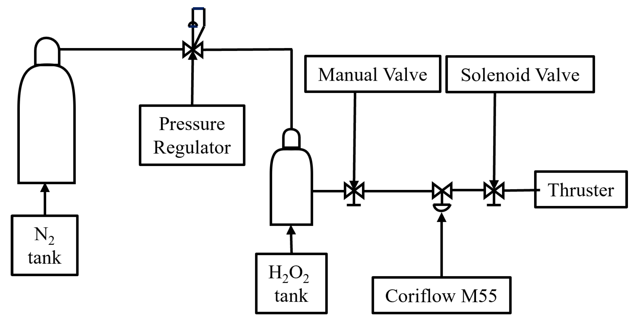
Figure 1. Laboratory feed line used for the experiments presented in this work [9].
Aerospace 12 00291 g001
Figure 2. Thruster assembly [9]. The red arrows indicate the position of each individual component that makes up the entire thruster.
Aerospace 12 00291 g002
Figure 3. Photo showing the fuel grains in ABS produced through 3D printing.
Aerospace 12 00291 g003
Figure 4. Logic scheme of the applied reconstruction technique.
Aerospace 12 00291 g004
Figure 5. Logic scheme of the performance calculation procedure.
Aerospace 12 00291 g005
Figure 6. Example of the computational grid used for the simulations in this work.
Aerospace 12 00291 g006
Figure 7. Regression rate vs. activation energy—linear interpolation. The two cyan-colored points indicate the regression rate obtained in the CFD simulations using the ABS properties derived from the literature, as shown in Table 3. The red square indicates the experimental regression rate value used to perform the linear interpolation on the line that connects the two cyan-colored points.
Aerospace 12 00291 g007
Figure 8. Regression rate vs. pre-exponential factor—linear interpolation. The two cyan-colored points indicate the regression rate obtained in the CFD simulations using the ABS properties derived from the literature, as shown in Table 3. The red square indicates the experimental regression rate value used to perform the linear interpolation on the line that connects the two cyan-colored points.
Aerospace 12 00291 g008
Figure 9. Fitted curves of the regression rate vs. the inverse of the average wall temperature; here, ‘X’ represents the values obtained via numerical simulations. The brown and gray lines represent the regression rate trends according to Arrhenius’ law, using the parameters from Table 3. The green line represents Arrhenius’ law with the parameters obtained through interpolation, the values of which are provided in Table 4.
Aerospace 12 00291 g009
Figure 10. Test measurements, showing example 3D-3. The black line indicates the oxidizer flow rate signal, the blue line is the pressure in the catalytic chamber, the yellow line indicates the pressure in the combustion chamber, and the green line indicates the thrust.
Aerospace 12 00291 g010
Figure 11. Experimental time-averaged characteristic velocities versus O / F . For all points and curves, the oxidizer is 87.5%-concentrated hydrogen peroxide. The red and black points refer to [29]. The continuous lines represent the theoretical trends of c in the case where the oxidant is injected entirely in the liquid state. The dashed lines represent the theoretical trends of c in the case where the oxidant is injected entirely in the gaseous state.
Aerospace 12 00291 g011
Figure 12. O / F versus time obtained by ballistic reconstruction. Each point represents the instantaneous value of O / F obtained by sampling the time at intervals of 0.1 s. All the points obtained from each individual test are combined with those from the other tests and displayed using the same color.
Aerospace 12 00291 g012
Figure 13. Regression rate laws. The green triangles represent the instantaneous regression rate values relative to the instantaneous mass flow. The values were obtained with a sampling interval of 0.1 s, and all points obtained from the different tests are displayed using the same color. The red dots represent the average regression rates obtained from the three experiments presented in Section 5.2, while the green and red curves respectively represent the power-law trendlines of the green and red points.
Aerospace 12 00291 g013
Figure 14. Photo of the tested fuel grains after longitudinal slicing.
Aerospace 12 00291 g014
Figure 15. Inner diameter profile, average inner diameter determined with the mass loss method, and average inner diameter measured by the caliper.
Aerospace 12 00291 g015
Figure 16. Contours of the static temperature and pathlines for simulated case 3D-1 (steady-state simulation).
Aerospace 12 00291 g016
Figure 17. Regression rate profile for simulated case 3D-1 (steady-state simulation).
Aerospace 12 00291 g017
Figure 18. Contours of mean mixture fraction for simulated case 3D-1 (steady-state simulation).
Aerospace 12 00291 g018
Figure 19. Case 3D-2 transient simulation at t = 0 s, showing the contours of the static temperature and pathlines.
Aerospace 12 00291 g019
Figure 20. Case 3D-2 transient simulation at t = 6 s, showing the contours of the static temperature and pathlines.
Aerospace 12 00291 g020
Figure 21. Grain port radius over grain length, showing the evolution in time and experimental inner radius profile for test 3D-2.
Aerospace 12 00291 g021
Table 1. Computational domain dimensions.
Pre-Chamber
Diameter
Pre-Chamber
Length
Fuel Grain
Length
Post-Chamber
Diameter
Post-Chamber
Length
23 mm15 mm40 mm16 mm10 mm
Table 2. Grid convergence analysis.
Mesh TypeCoarseReferenceFine
r ˙ n u m , mm/s0.4300.4870.493
G C I f i n e , %////0.179
G C I c o a r s e , %1.720////
Table 3. Solid fuel properties and rate constants.
Fuel Type ρ [kg/ m 3 ] C p [J/kg K] h p [MJ/kg]A [mm/s] E a [kJ/mol]
Extruded ABS102527140.231423.3362.14
FDM ABS97127140.24265494.18113.44
Table 4. Properties and rate constants of the interpolated model of 3D-printed ABS.
Fuel Type ρ [kg/ m 3 ] C p [J/kg K] h p [MJ/kg]A [mm/s] E a [kJ/mol]
ABS 3D Printed120027140.231487.75074.622
Table 5. Operating conditions and thruster configuration.
Test 3D-1Test 3D-2Test 3D-3
Feeding pressure, bar19.62429.4
Expected oxidizer mass flow rate, g/s22.53.5
Grain length, mm404040
Initial port diameter, mm9.3359.549.56
Nozzle throat diameter, mm2.12.12.1
Area ratio3.8123.8123.812
Injector diameter, mm222
Table 6. Experimental test results.
Test3D-13D-23D-3
Duration, s777.2
Δ M , g6.59 ± 0.018.19 ± 0.019.31 ± 0.01
Ch. pressure, bar16 ± 0.0719.5 ± 0.0723.6 ± 0.07
c , m/s1889.73 ± 191.061859.65 ± 151.751742.55 ± 110.18
Thrust, N5.36 ± 0.056.9 ± 0.058.7 ± 0.05
O / F ¯ 2.16 ± 0.322.15 ± 0.262.68 ± 0.23
G ¯ ox , kg/m2 s15.74 ± 2.3217.56 ± 2.1022.48 ± 1.95
m ˙ ¯ fuel , g/s0.94 ± 0.0011.17 ± 0.0011.29 ± 0.001
m ˙ ¯ ox , g/s2.03 ± 0.00062.51 ± 0.00073.46 ± 0.0007
m ˙ ¯ tot , g/s2.97 ± 0.33.68 ± 0.34.75 ± 0.3
r ˙ ¯ , mm/s0.50 ± 0.0010.56 ± 0.0010.62 ± 0.001
D p , in , mm9.3359.549.56
D ¯ p , mm12.82 ± 0.0113.49 ± 0.0114.00 ± 0.01
D ~ p , fin , mm16.30 ± 0.0117.44 ± 0.0118.44 ± 0.01
Table 7. Results predicting the performance of the engine using the regression law of the green line (Figure 13) and percentage error with respect to the experiment.
Test3D-1
Code
Err %3D-2
Code
Err %3D-3
Code
Err %
O / F ¯ 2.222.782.4313.022.804.48
G ¯ ox , kg/m2 s16.072.1018.887.5223.956.54
m ˙ ¯ fuel , g/s0.913.191.0311.971.234.65
m ˙ ¯ tot , g/s2.941.013.543.804.691.26
r ˙ ¯ , mm/s0.484.000.527.140.603.23
D ¯ p , mm12.681.0913.013.5613.563.14
D ~ p , fin , mm16.021.7216.694.3017.793.52
Table 8. Results predicting the performance of the engine using the regression law of the the red line (Figure 13) and percentage error with respect to the experiment.
Test3D-1
Code
Err %3D-2
Code
Err %3D-3
Code
Err %
O / F ¯ 2.064.632.265.122.622.24
G ¯ ox , kg/m2 s15.581.0218.284.1023.193.16
m ˙ ¯ fuel , g/s0.984.261.115.131.322.33
m ˙ ¯ tot , g/s3.011.353.621.634.780.63
r ˙ ¯ , mm/s0.502.000.551.790.631.61
D ¯ p , mm12.880.4713.222.0013.781.57
D ~ p , fin , mm16.420.7417.101.9518.231.14
Table 9. Computed average wall temperature and relative error between the experimental and numerical average regression rates for all tests.
Test3D-13D-23D-3
Numerical Average Wall T, K863.14874.62900.30
Experimental Average Regression Rate, mm/s0.500.560.62
Numerical Average Regression Rate, mm/s0.490.520.60
Regression Rate Relative Error, %2.66.92.9
Table 10. Relative error between the experimental and numerical average regression rates computed with the mass loss method for test 3D-2.
r ˙ ¯ exp , mm/s r ˙ ¯ num , mm/sRelative Error, %
0.560.5256.25
Disclaimer/Publisher’s Note: The statements, opinions and data contained in all publications are solely those of the individual author(s) and contributor(s) and not of MDPI and/or the editor(s). MDPI and/or the editor(s) disclaim responsibility for any injury to people or property resulting from any ideas, methods, instructions or products referred to in the content.