Abstract
In recent years, advanced nozzle concepts have attracted interest because of advancements in their technology readiness level and studies on applications to vertical take-off and landing reusable launch vehicles. This is ascribable to their intrinsic altitude compensation properties, which could mitigate the additional propellant cost resulting from the vertical landing manoeuvres based on retro-propulsion. Experimental and numerical campaigns at the Technical University of Dresden test the performance of annular-aerospike, dual-bell, and expansion-deflection nozzles compared with conventional bell-shaped nozzles in various subsonic counter-flow regimes and atmospheric conditions. The methods of investigation and a detailed description of the experimental and numerical results are reported. More specifically, the study offers a comparison between advanced and conventional nozzles, with a focus on nozzle performance through experiments and aerodynamic performance and retro-flow interaction through simulations. The flow topology that is established within the area of interaction between nozzle jets and counter-flows is detailed, with the advantages and limitations of each advanced nozzle in terms of adaptive performance. The numerical simulations confirm that advanced nozzles achieve altitude compensation in retro-flow configurations. Moreover, the distance obtained from the models for jet penetration into subsonic counter-flows is compatible with empirical formulations available in the literature.
1. Introduction
State-of-the-art reusable main-stages for heavy-lift launchers perform vertical landing through retro-propulsion (e.g., Falcon 9 and Falcon Heavy by Space X). Such an approach lowers the cost of payload mass to orbit for customers [1,2,3] and increases the number of launches per year by providers [4,5,6]. This radically changed the capabilities of access-to-space and raised the interest towards the physics of retro-propulsion as well. The current class of reusable launch vehicles (RLVs), as developed by private companies as Space X and Blue Origin, envisaged the adoption of bell-shaped nozzles. However, the novel scenario of vertical landing through retro-propulsion encourages the scientific community to question the effectiveness of bell-shaped nozzles as the optimum solution. Indeed, the additional propellant required for the recovery manoeuvres still poses a limit to available payload per launch. Moreover, novel critical phenomena arise during the supersonic retro-propulsion (SRP), such as recirculation areas at the base plate, re-ignition difficulties due to external counter-flows, plume–plume, plume–shock and shock–shock interactions, flow separation and side-loads, high thermal loads at side-walls, and many others [7]. In this regard, advanced nozzle concepts (ANCs) might solve these drawbacks, together with higher performance in vacuum operations thanks to their intrinsic altitude compensation [8]. At Technische Universität Dresden (TUD), recovery strategies based on retro-propulsion for Vertical Take-Off Vertical Landing reusable launch vehicles (VTVL-RLVs) are investigated through experiments and numerical simulations. These studies involve the design and development of advanced nozzle models, such as aerospike, dual-bell, and expansion-deflection [9]. The main interest is evaluating the effectiveness of the altitude compensation of the ANCs during subsonic retro-propulsion. This is achieved through numerical simulations in Ansys© Fluent (2024 R2), together with an experimental campaign in parallel [10,11]. This manuscript offers a description of such a CFD study; it introduces the reader to the topic of retrorocket exhausts in subsonic counter-flows in Section 2 and describes in detail the numerical models and proposed methodology in Section 3. The numerical results are reported in Section 4 and then verified and validated with experimental results in Section 5. Then, the results are discussed quantitatively (performance comparison and comparability with predictive models) and qualitatively (flow comparison with schlieren pictures) in Section 6. In conclusion, the limits of the proposed methodology and results, together with an overview of future activities, are provided in Section 7.
2. Theoretical Background
The Powered-Descent Landing (PDL) manoeuvres for vertical landing of main-stages, as introduced by SpaceX and their Falcon programme, define the standard of the current class of reusable launch vehicles. PDL introduces benefits in terms of extension of recovery, minimisation of time for refurbishment, and reduction in cost per launch [8]. Nevertheless, there are aspects of the physics of retro-propulsion that still constitute a challenge because of its novelty for the recovery of boosters and main-stages. This section summarises the main concepts behind retro-propulsive landing, the adopted methodology of investigation, and the application of advanced nozzles to these novel recovery strategies. This specific field of application of advanced nozzles (powered vertical landing of RLVs) still offers a rather scarce literature. Thus, the latest advancements on predictive methodologies are introduced only for subsonic retro-propulsion in Section 2.1 and contextualised to RLV applications in Section 3.
2.1. Subsonic Retro-Propulsion
Any landing manoeuvre with active retro engines experiences complex interactions between plumes and the external counter-flow, which determine the flow topology of the area of interaction, namely the Aerodynamics Interference (AI) area [12]. Nowadays, the description of such phenomena is derived via extensive CFD campaigns, mostly by adopting Reynolds Averaged Navier Stokes (RANS) time-averaged equations of motion for fluid flow in combination with Shear-Stress Transport (SST) turbulence models [13] (more details in Section 3), but recently the research provided a better understanding of the flow structures and scalability factors through experimental activities, together with insights on the aerodynamic performance of the vehicle during the re-entry. This was performed for supersonic retro-propulsion (SRP) and subsonic retro-propulsion (SubRP) by NASA [12] and DLR [14]. In this case, the terms “supersonic” and “subsonic” refer to the Mach regime of the atmospheric counter-flow. In particular, Marwege et al. [14] experimentally verified an empirical formulation for the estimation of the plume length x normalised with the nozzle exit diameter , originally provided by NASA and valid for SubRP [14,15]:
where is a factor that varies from [14] to [15] (depending on the experimental setup), and the first and last parentheses represent the momentum flux ratio, or , between the nozzle exit and asymptotic free-stream, and the temperature ratio () between the combustion chamber and nozzle exit, respectively. Equation (1) exhibits direct proportionality with the square roots of and , which indicates that they are important similarity parameters to be considered in experiments that simulate retro-propulsion manoeuvres (together with the ambient pressure ratio, or ) [14]. Similar studies were also conducted through experiments by JAXA in the context of feasibility studies for VTVL single-stage-to-orbit vehicles [16], with a focus on aerodynamic drag coefficient and pressure coefficients. To define these during a retro-propulsion manoeuvre, the analysis of aerodynamic performance distinguishes between nozzle jet contribution and aerodynamic contribution for both the overall drag (D) and drag-coefficient () [12,17]. More specifically,
where is the effective thrust resulting from the interaction between the nozzle jet and free-stream, is the contribution of aerodynamics to the drag (i.e., viscous-drag, induced-drag, wave-drag), is the dynamic pressure of the free-stream (), and the reference area is commonly the cross-sectional area of the vehicle ().
Equations (3) and (4) define the aerodynamics-thrust-coefficient [12] (, not to be confused with the nozzle-thrust-coefficient or [18]) and the aerodynamic-drag-coefficient (), respectively. Alternatively, the momentum ratio between the nozzle jet and free-stream, namely the multiplied by , can substitute if the pressure loss in the thrust is neglected [19]. Overall, the parameters in Equations (3) and (4) describe the contribution of propulsion and aerodynamics to the total drag for various regimes of dynamic pressure during a retro-propulsion manoeuvre, respectively.
Nonaka et al. describe the physics of SubRP in a punctual manner [16]: as the nozzle jet encounters a subsonic free-stream, an axisymmetric recirculation region (AI area) arises. The recirculation flow becomes more extensive for higher ; subsequently, the aerodynamic drag () decreases, while the overall drag (D) increases due to the thrust contribution of the nozzle. This mechanism of aerodynamic drag reduction is determined by the recirculation region formed by the jet/free-stream interaction, as the free-stream flow to the base surface is blocked. Consequently, the surface pressure on the base area drops rapidly. In contrast to Nonaka, Marwege et al. focused their attention on the flow topology and its steadiness, reporting that a supersonic jet exhausting into the free-stream shows strong unsteady behaviour for above and sea-level standard (SLS) atmospheric conditions [14]. During a subsonic retro-propulsion, the flow topology and its steadiness is strongly influenced by the aforementioned MFR and by the ambient pressure ratio (). More specifically, MFR describes the interaction between nozzle jets and counter-flow by scaling the jet plume length [15], while APR determines the flow structure at the nozzle exit [20]. The contributions of the MFR and APR appear in the aerodynamic-thrust-coefficient , reformulated in explicit form as follows [17,21]:
where and are the nozzle-exit-area and the exit-Mach-number, respectively, while and are the adiabatic indexes for plumes and counter-flow. In Equation (5), the APR () and the form-factor appear from manipulating the definition of and thrust [21].
Finally, to derive the aerodynamic drag, the pressure coefficients () are integrated over the body. In axisymmetric 2D models, they are defined as follows:
where is the local static pressure at any given point on the surface of the vehicle, and the other quantities refer to the asymptotic free-stream.
2.2. Advanced Nozzles in Subsonic Counter-Flows
In recent years, the penetration of retrorocket exhausts into supersonic counter-flows (i.e., SRP) has found renewed interest in applications for reusable rockets recovery. Much work has been published on this topic in the past, but there is still limited information available on subsonic retro-propulsion (SubRP) [15], which characterises the powered vertical landing phase. This is because the interaction during a SubRP is unstable; the nozzle jet behaves in long penetration mode [14] and tends to dissipate by mixing [16]. This differs substantially from a SRP, in which the nozzle jet can be contained within the bow-shock resulting from interaction with the supersonic free-stream. During a SRP, the interaction between the counteracting flows can result in a more stable Short Penetration Mode (SPM, or blunt mode) above certain values of (transition usually occurs for ) [12,21]. Equation (5) shows the impact of momentum flux ratio, ambient pressure ratio, and form-factor on . The latter is generally considered to be the main parameter for characterising the interaction between retro-jet and counter-flow [17,21].
In this regard, advanced nozzle concepts (ANCs) (e.g., aerospike, dual-bell, and expansion-deflection nozzles) [9] allow higher degrees-of-freedom in designing the exit conditions and form-factors of the nozzles to achieve higher performance at more stable retro-flow configurations [8]. Indeed, the ANCs potentially offer an overall better performance than conventional bells over various flight conditions because of their inherent altitude compensation capability. In addition, they can achieve higher expansion ratios at smaller volumetric encumbrances, and some of them (i.e., aerospike engines) can share major structural components with the vehicle itself so that the overall weight of the vehicle is reduced significantly. Moreover, alternative solutions to gimballed thrust systems could be achieved in the specific case of a clustered aerospike, as the modular combustion chambers can be operated individually. This feature allows for the manoeuvring of the vehicle through differential throttling during ascent phases and retro-propulsive regimes [22,23]. A more detailed description of the advanced nozzles considered for this study, together with their specific altitude compensation principles and their application to reusable main-stages, is available in references [8].
On the other hand, as the altitude compensation requires the nozzle jet to adapt to the ambient condition, their effective performance is very sensitive to the outer free-stream. This implies that the efficiency of compensation must be verified experimentally before claiming that they are suitable for retro-propulsion. The literature is scarce in this regard, except for a numerical study by Ghosh et al. [24] that proves the annular-aerospike concept to be suitable also for SRP applications, but no research has been pursued at high technology-readiness-level on ANCs for vertical landing manoeuvres. This condition is particularly critical because of the interaction of the denser atmospheric layers with the aerodynamic boundaries of the jet, which defines both the efficiency and predictability of the altitude compensation itself. Therefore, this paper investigates the effectiveness of altitude compensation of advanced nozzles, as well as the flow topology in both counter-flow/retro-flow configurations, through numerical analysis supported by an experimental campaign in parallel. The latter is addressed in Section 5.2, and is reported in more detail in previous publications by TUD [10,11].
2.3. Nozzle Performance
The performance of the nozzle is evaluated in terms of several parameters. First of all, the thrust is considered, as it coincides with the axial force () at null-AoA and in the absence of thrust vectoring. Furthermore, the nozzle thrust coefficient () and specific impulse () are also evaluated to complete the characterisation. To evaluate the thrust of conventional and advanced nozzles, the following Equation [25] is considered.
where is the mass-flow, and and are the average static pressure and flow velocity at the nozzle exit, while is the ambient pressure. The and are the cross-sectional areas of the nozzle exit and throat, respectively. Equation (7) considers both the momentum contribution and the adaptation to the ambience (both contributing to the ). This equation is adopted for the evaluation of T and for most cases, except the aerospike nozzle (AN). Indeed, for the AN a dedicated expression needs to be implemented [25,26].
The first term of the sum represents the axial component of the thrust evaluated at the exit section of the AN (it coincides with the throat for this specific design). This thrust contribution is calculated as projection of the thrust vector obtained through Equation (7) onto the plug axis. For plug nozzles, this turning angle (, angle between plug axis and sonic line on a pure external expansion plug nozzle) depends on the design methodology assumed for contouring. The second term in Equation (8) is the integral of the pressures acting on the spike over the axially projected area normal to the plug axis. The final term is the pressure acting over the base area and represents the contribution of the base pressure for truncated plug nozzles. The latter spans from a small drag or neutral contribution during open-wake regimes, highest losses during transition between operative modes, to positive values at lower ambient pressures [22].
The last parameters used to describe the nozzle performance are the nozzle-thrust-coefficient () and specific impulse (), derived as follows [18]:
The equations introduced here are adopted in Section 4.1 to evaluate the performance of each nozzle in three different scenarios: performance at design point (PRF-OD), at sea-level standard conditions (PRF-SLS), and performance in retro-flow configuration (RFL).
3. Methodology
The numerical models used as methods of investigations, together with a brief introduction to the advanced/conventional nozzles and case studies considered, are presented in this section.
3.1. Geometries
The design approaches for each specimen are here provided, together with their CAD models in Figure 1. In analogy to the test specimens studied within the experimental campaign, three different advanced nozzles designed for near-vacuum operations ( km, = 10.7 kPa) were investigated for this CFD study: the annular aerospike nozzle (AN), dual-bell (DB), and expansion-deflection (ED) nozzles. In addition, a conventional Rao-bell parabolic nozzle (RAO-bell) designed for near to sea-level standard (SLS) conditions is included ( km, = 34.7 kPa). Such a nozzle is adopted as a reference for performance in retro-flow configuration at SLS to highlight the performance gains during landing manoeuvres of ANCs due to their intrinsic altitude compensation properties at higher expansion ratios. As the investigation involves only axisymmetric geometries, all analyses are conducted on simplified two-dimensional models in axisymmetric domains.
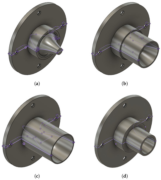
Figure 1.
CAD models of advanced and conventional nozzles: (a) aerospike nozzle (AN), (b) dual-bell (DB) nozzle, (c) expansion-deflection (ED) nozzle, and (d) Rao-bell parabolic nozzle (RAO-bell).
For the AN, the C. C. Lee ideal contour design method [27] is adopted (singular annular throat), with a truncation length of 45% of the ideal profile and sonic conditions at the exit (only external supersonic expansion). In this configuration, the performance losses due to truncation should be below 5%; these losses could be reduced by including 1–2% of the total mass-flow for the base-bleed [22].
The DB nozzle offers a step-wise altitude compensation, which results from the combination of two different optimal expansion points. The core nozzle is a Truncated Ideal Contour (TIC) designed at near-SLS condition, while the nozzle extension is a Constant Pressure (CP) at the nozzle wall contour, designed for near-vacuum as the other ANCs. The TIC design is derived through an in-house design tool developed at TUD based on ideal expansion with a Method Of Characteristics (MOC), then truncated at the same exit angle of the RAO-bell nozzle (5.25°). This cut corresponds to of the ideal contour length. In order to generate the CP contour for the extension, a 2D simulation of the TIC nozzle operating at 10,670 Pa ambient pressure was performed. Starting from the exit section of the TIC, an isobar curve at 10,670 Pa over the expanding plume was derived numerically, and this curve was then truncated at the same expansion ratio (, with and being the nozzle exit and throat areas, respectively) of the other ANCs. The selected sharp inflection angle measures 21.75°, while the relative length of the nozzle extension (ratio of nozzle extension length over total length of the DB nozzle) measures ca. , close to the optimum values suggested in the literature [28]. The expansion ratio of the TIC results is lower than the RAO-bell for near-SLS (, instead of ) in order to match the desired inflection angle and relative length of the extension.
The ED nozzle was designed by adopting a modified version of the original Angelino’s design-method [22] for ideal contouring of ED nozzles. It presents a higher expansion ratio with respect to the other ANCs (, instead of ). This was a deliberate design choice, as the performance of ED nozzles is penalised by the presence of a central pintle; thus, the design was adapted to match the same average exit-Mach-number of the other ANCs at design point [11]. The ED nozzles are also known for their high losses due to aspiration drag at sea level [29]. Nevertheless, the ED nozzle was included in the comparative analysis to investigate its effective altitude compensation against free-streams.
The conventional nozzle adopts a classic Rao-parabolic-contour, in agreement with the design parameters suggested in the literature [18]. It presents an 80% length with respect to its equivalent conical nozzle (in terms of , throat geometry, and chamber conditions for each). The design point considers a lower on-design with respect to the ANCs (, instead of , ca. 69% lower), as it is optimised for an altitude point in standard conditions close to a Merlin 4D engine. A lower geometrical expansion ratio with respect to the ANCs (, instead of ), at identical chamber conditions, allows for quantifying the performance gains of advanced nozzles adapted for vacuum when operating in SLS conditions. Additionally, this study evaluates these performance gains in combination with subsonic free-streams.
The nozzle models presented here are simulated by setting identical chamber conditions for all simulations. The selected working fluid is dry-air at standard ambient temperature. To better clarify the similarities between the different nozzle specimens, an overview of the design parameters chosen for the ANC models is offered in Table 1.

Table 1.
Reference design parameters for advanced nozzles [10].
The flow domain adopts a simplified geometry for the reusable main-stage as a cylinder with a length () of mm and a diameter () of mm, resulting in an aspect ratio () of . This is a compromise between real-case applications (e.g., Falcon 9 landing manoeuvres) and the limits of the test-bench for the experimental campaign [11]. This is acceptable, as well as the absence of aerodynamic disturbances (e.g., landing legs), as the focus of this study is to investigate the interaction between the nozzle jet and free-stream, rather than replicate a retro-flow experiment over a complete model of the stage. A body-to-nozzle diameter ratio () of approximately is selected, close to values for the octa-web configurations of a Falcon 9; the latter is a crucial parameter during SRP [12], since it also influences the form-factor () in Equation (5).
Figure 2 shows the geometry in the presence of subsonic counter-flows. Previous CFD studies [30] proved a distance of mm to be sufficient to capture the stagnation point, at a null Angle of Attack (AOA) and for the considered, without negative influence by the boundaries. In general, it is advisable to enlarge the flow domain enough to capture the interaction with the nozzle jets correctly. The domain is extended to best match the experimental conditions, therefore the vertical distance from the symmetry-axis is expanded to mm, in conformity to the actual dimensions of the vacuum wind tunnel (refer to Section 5.2). The flow field considered excludes the evaluation of any wake drag (the left boundary in Figure 2 is limited to the length of the body), thus it is not fully representative of a real case. Nevertheless, it should be clear that the focus of this study is to reproduce with accuracy the area of interaction between the nozzle jet and free-stream, rather than replicate a retro-flow experiment. This is meant as a compromise between a realistic solution and computation effort, due to a large number of simulations.
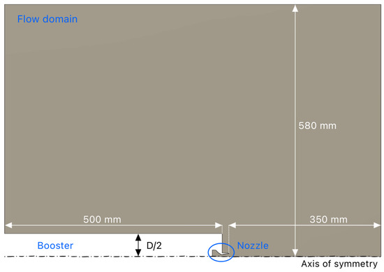
Figure 2.
Geometrical domain of the flow-field for counter/retro-flow cases.
3.2. Model Properties
The numerical models are based on Reynolds Averaged Navier Stokes (RANS) steady equations of motion for fluid flow, a reduced form of the general Navier–Stokes equations. In the RANS approach, the governing equations describe the average flow field and the effects of the unsteady fluctuations are modelled. This requires an additional turbulence model to account for the evaluation of the Reynolds stresses which represent the effect of the unresolved fluctuations on the averaged field. In this case, the SST is selected, and the details of the closure model are further discussed in Section 3.5. In RANS modelling, the Navier–Stokes equations are time-averaged, thus the time derivative disappears from the RANS equations: since the characteristic time of the nozzle fluid dynamics is significantly smaller then the re-entry time, it is possible to study the problem with a sequence of steady simulations. This choice constitutes a compromise between the accuracy of the solution and computational time due to the high number of simulations. Alternative methods include Unsteady-RANS with increasing pressure over time to better resemble the decreasing altitude during a powered vertical landing manoeuvre (discussed further in Section 7). The model properties are identical between the simulations, in order to compare the results consistently (refer to Table 2).
Table 2.
Model properties for the numerical simulations in Ansys© Fluent.
Occasionally, some minor adjustments were made to the original models (e.g., starting the solution with a first-order method or modifying the higher-order term relaxation value). The choice of a pressure-based solver (instead of density-based, originally designed for high-speed compressible flows) comes from the specific need to simulate nozzle jets immersed in subsonic counter-flows. In this scenario, the aerodynamic characteristics of the external flow field are determined by incompressible and mildly compressible flows, thus suggesting the adoption of a pressure-based solver. Nowadays, the inclusion of pressure work and kinetic energy terms (often negligible in purely incompressible flows) allows modern pressure-based approaches to be applicable to a broad range of flows (from incompressible to highly compressible). Indeed, modern solvers like Ansys© Fluent automatically account for pressure work and kinetic energy in case of modelling compressible flows or modelling incompressible flow with viscous dissipation and the pressure-based solver [31]. Additionally, the selected approach is supported by a previous study within the research group (in collaboration with DLR Lampoldshausen) [32], which confirms a correct depiction of highly compressible nozzle jets with coupled pressure-based solvers, both in terms of flow-field topology and pressure distributions over the spike.
3.3. Boundary Conditions
Four different cases of interest have been identified for each nozzle:
- Nozzle Performance On-design (PRF-OD): delivers the performance of the nozzle at its specific design point, validated through experiments;
- Nozzle Performance Off-design (PRF-SLS): delivers the performance at sea-level standard (SLS), validated through experiments;
- Aerodynamic Performance in Counter-flow (CFL): delivers the aerodynamic drag at SLS in the absence of nozzle jet, validated through data available in the literature;
- Nozzle and Aerodynamic Performance in Retro-flow (RFL): delivers the total and aerodynamic drags at SLS in the presence of nozzle jet, validated through data available in the literature.
For each case in the previous list, the boundary conditions are set. In all cases, for the base plate and side-walls of the booster, as well as for the inner walls of the nozzle, the boundary type is always set to no-slip “wall”. The axis of symmetry is set to the homonym boundary type. Instead, the remaining four boundaries of the flow field (see Figure 3) are differentiated between each case. They are presented in detail in Table 3, Table 4, Table 5 and Table 6.
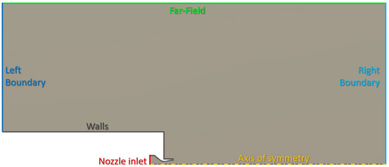
Figure 3.
Boundary regions in the simulations.
Table 3.
Boundary conditions for nozzle performance on-design (PRF-OD case).
Table 4.
Boundary conditions for nozzle performance off-design (PRF-SLS case).
Table 5.
Boundary conditions for aerodynamic performance in counter-flow (CFL).
Table 6.
Boundary conditions for nozzle and aerodynamic performance in retro-flow (RFL).
By setting the operating pressure to 0 Pa, all gauge pressure values are identical to the local static pressure. For the CFL and RFL cases, a far-field velocity inlet is adopted. Generally, a far-field velocity inlet can also be used for compressible flows [31], though not always recommended, as the total pressure is not fixed but increases to provide the prescribed velocity distribution. This deliberate choice (instead of a more classical combination of pressure inlet/outlet) comes primarily from the need to ease the convergence of the solution in the presence of a low Mach uniform and counteracting free-stream. However, the two approaches are equivalent for this specific case, since the average total pressure at the inlet is verified in practice to coincide with the prescribed ambient pressure.
3.4. Meshing
The discretisation of the flow-field results in a structured mesh of quadrilateral elements, generated by applying to every edge an appropriate number of subdivisions (see Figure 4). As a general approach to meshing, preliminary requirements for global meshing quality are defined a priori to achieve satisfactory standards. These include average orthogonality, average skewness, and average aspect ratio. The global parameters always reached their target value for all the cases considered (refer to Table 7). In addition, a minimum number of cells (500 k) is assumed for all scenarios, with the exception of RFL cases (double number of cells, higher resolution both for the nozzle and the booster walls, see Figure 5). For a correct depiction of the boundary layer (BL) region, specifically the viscous sublayer, the value is checked to be lower than 5, which is still an acceptable upper limit for SST turbulence models [33]. Occasionally, this value needs to be refined in specific critical areas, such as the inflection point of the DB nozzle (with a target value of 1.5). The discretisation approach included mesh sensitivity study through multiple refinement iterations. Firstly, simulations performed with a tentative mesh provided a preliminary evaluation of flow performance or key features, allowing for the quick identification of issues and initial modifications associated with a sustainable computational cost. Then, a manual mesh refinement optimised quality and resolution, leading to more accurate results and enhancing the resolution of flow characteristics of interest. In general, this multi-phase approach in CFD simulations combines efficiency, cost reduction, and improved accuracy.
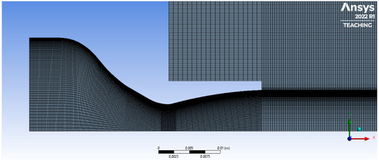
Figure 4.
Discretisation grids (RAO-bell, PRF case) after mesh refinement.
Table 7.
Meshing target values for key parameters.
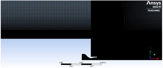
Figure 5.
Discretisation grids (RAO-bell, RFL case) after mesh refinement.
3.5. Turbulence Modelling
The turbulence model selected is the Shear-Stress Transport (SST) [34], a two-equation eddy-viscosity model that couples a formulation within the boundary layer with a model for the free-stream, thus combining the best of the two models. This turbulence model performs well against adverse pressure gradients and separated flow. Alternative methods in the literature include hybrid models, such as the Large-Eddy Simulation (LES) adopted by Ghosh et al. [24]. However, a SST constitutes an acceptable compromise to obtain reliable results at a low computational effort [26,32].
4. Numerical Results
In this section, the results for both the nozzle performance and the aerodynamic performance of the body are reported. A more detailed discussion of the results is provided in Section 6.
4.1. Nozzle Performance
The performance of each nozzle is evaluated in three different scenarios: at the design point (see Table 8), at sea-level standard conditions (see Table 9), and in retro-flow configuration (see Table 10). The first reveals the performance on-design and weights the impact of a higher geometrical expansion ratio for the ANCs, the second evaluates their altitude compensation capabilities at standard ambient conditions with respect to a conventional nozzle, and the last case is compared to the performance in SLS to determine the efficiency of their altitude compensation capabilities, also against subsonic free-streams.
Table 8.
Results for the evaluation of nozzle performance at each specific design point (PRF-OD: MPa).
Table 9.
Results for the evaluation of nozzle performance at SLS ambient conditions (PRF-SLS: MPa).
Table 10.
Results for the evaluation of nozzle performance during subsonic retro-propulsion (RFL: MPa, m/s uniform, ambience at SLS).
The results in Table 8 and Table 9 offer the information needed for the validation of the models with the experimental data for each nozzle, operating at its specific design point and at SLS conditions, respectively. A first analysis under SLS conditions shows that both AN and DB nozzles (designed for near-vacuum) perform better than the conventional RAO-bell nozzle (designed for near-SLS) because of their intrinsic altitude compensation, despite having a higher expansion ratio. Moreover, the aerospike achieves an almost optimal altitude compensation (). In Figure 6, Figure 7, Figure 8 and Figure 9, examples of CFD post-processing are offered to better visualise the principle of altitude compensation for the AN and DB nozzles.
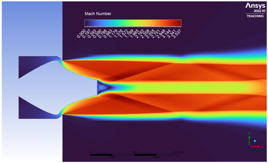
Figure 6.
Flow visualisation (Mach contours) for AN at design point ().
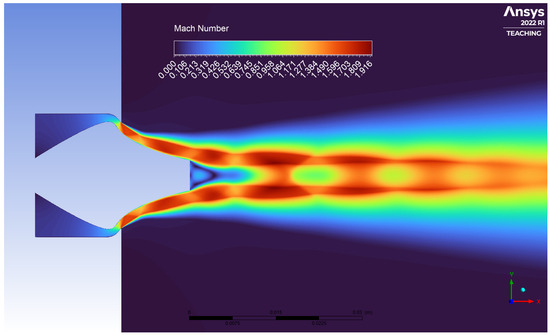
Figure 7.
Flow visualisation (Mach contours) for AN at SLS ().
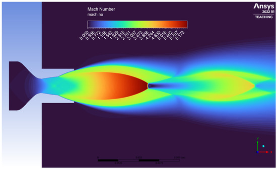
Figure 8.
Flow visualisation (Mach contours) for DB nozzle at design point ().
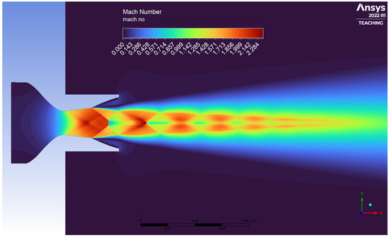
Figure 9.
Flow visualisation (Mach contours) for DB nozzle at SLS ().
In Table 10, the results for the evaluation of the nozzle performance in retro-flow configuration (RFL) are provided. The information needed for evaluating the effective altitude compensation achieved by the advanced nozzles, while invested by a subsonic counter-flow, can be derived from here. For the case study considered, the nozzles operate against a low-subsonic free-stream (, incompressible-flow regime) at null-AOA. In this case, all the ANCs preserve their altitude compensation capabilities; in addition, all nozzles perform better in RFL with respect to PRF-SLS, thanks to a higher . This comes from deriving the through the static pressure of the free-stream (), instead of the stagnation pressure (). This assumption underestimates the static pressure at the nozzle exit, formerly corresponding to the average static pressure within the recirculation region ( or dead air pressure). At the base plate, it should result in during a subsonic retro-propulsion, because locally the pressure is subject to the residual momentum of the free-stream and large vortexes within the recirculation area. The results in Table 10 and their implications are further discussed in the dedicated Section 6.
4.2. Aerodynamic Performance
In this section, first the aerodynamic performances of the models against a subsonic free-stream (CFL) are offered. Table 11 reports the aerodynamic performance in terms of aerodynamic drag and total drag coefficients. The only contributions to the total drag are the viscous-drag (skin-friction) and the pressure drag at the base plate, in the absence of the nozzle jet. A first analysis shows that the form-factor of the nozzles had a limited impact over the aerodynamics of the launcher in the absence of retro-propulsion and for relatively small expansion ratios involved. An example of CFD post-processing for a counter-flow configuration is available in Figure 10.
Table 11.
Numerical results for aerodynamic performance of the body against a subsonic free-stream (CFL: m/s uniform, ambient conditions at SLS).
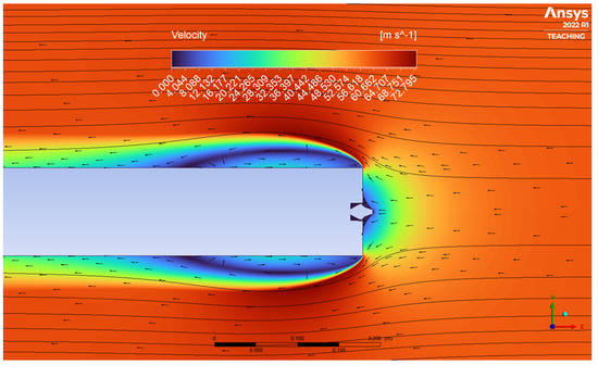
Figure 10.
Flow visualisation (velocity contour with streamlines) for AN in CFL ( m/s).
The first observations involve the pressure coefficients in Table 11: the pressure coefficient at the base plate () reaches almost unity, thus representing an area of stagnation conditions (maximum pressure drag). The closeness to complete stagnation conditions (bluntness of the extended body) depends also on the form-factor of the nozzle. For example, the sharpness of the aerospike seems to reduce the aerodynamic drag at the base. On the contrary, the pressure coefficient at the side-wall () decreases independently from the nozzle type, since the flow separates at the base plate.
In Table 12, the results for the aerodynamics of retro-flow configurations (RFL) are reported. In case of subsonic retro-propulsion, the flow separation at the base plate does not occur because of the interaction with the nozzle jet. The flow-reattachment at the side-walls () is verified for all the nozzles. Such behaviour is common between all cases, thus it is not influenced by the form-factor of the nozzle. In this specific case, the models are invested by a subsonic free-stream and the nozzle operates under SLS ambient conditions. The values report the length of jet penetration in the subsonic free-stream, defined as the distance between the base plate and the stagnation point (, for null-AOA) of the nozzle jet. The results in Table 12 show similar decrements in the aerodynamic drag between the nozzles. This indicates that thrust is not necessarily the dominant factor for the reduction in aerodynamic drag. The pressure coefficients at the base indicate that the base plate does not present stagnation conditions () due to the presence of recirculation areas; this verifies the tendency towards higher , as discussed in Section 4.1. This happens because the average pressure over the base plate depends on the dead air pressure () within the recirculation region. This value is lower than ambient pressure (), and depends on both longitudinal jet penetration distance and radial extension of the AI region; in other terms, it depends on the momentum flux ratio () and ambient pressure ratio (). In this case, the ED presents the highest geometrical expansion ratio and the shortest jet penetration distance, while the core nozzle of the DB operates close to optimum expansion and presents the longest . In spite of this, the ED nozzle still experiences a lower static pressure, , instead of ≈−56%). This result suggests that the ambient pressure ratio () had an impact on the aerodynamic pressure drag at the base plate greater than the momentum thrust or jet penetration distance. This can be correlated to the dependency of the radial extension of the AI region from the same parameter. An example of CFD post-processing for a retro-flow configuration is available in Figure 11.
Table 12.
Numerical results for aerodynamic performance of the body in subsonic retro-flow configuration (RFL: m/s uniform, ambient conditions at SLS).
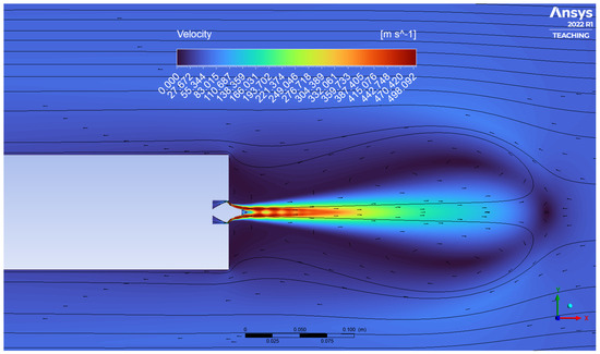
Figure 11.
Flow visualisation (velocity contour with streamlines) for AN in RFL ( m/s).
5. Verification and Validation of Simulations
This section is dedicated to the verification of numerical models with preliminary calculations and to validation through comparison with experimental results and background-oriented schlieren (a description of the experimental setup is included).
5.1. Verification Process
The verification process develops in two steps: a comparison between numerical and analytical calculations to verify the performance of each nozzle at various nozzle pressure ratios and the physics of the subsonic retro-propulsion; and the verification of convergence criteria for the simulations.
Table 13 presents a comparison between ideal performance values, calculated analytically during the preliminary design phase and referred to the design point of each nozzle (optimum expansion). The numerical results fall confidently within 5–7% less thrust with respect to their ideal case. Such a margin is compatible with the losses induced by the non-linear phenomena on the nozzle flow (e.g., non-ideal contours, viscous-drag, non-optimal expansion, divergence losses) [18]. The performance of the simulations are always achieved at lower mass-flows compared to the ideal case (). This counter-intuitive result could account for the low Reynolds numbers at the throat (cold-flows) that enlarge the boundary layer and reduce the effective throat area, thus reducing the mass-flow/thrust with respect to an ideal case. Despite this, the simulations show good agreement with the expected performance and estimation of losses, which verifies the physics of the models at their design point.
Table 13.
Verification of performance at design point (losses with respect to ideal performance of each nozzle derived analytically in hypothesis of quasi-1D isoentropic nozzle flow [18]).
Insights into the altitude compensation of the advanced nozzles can be deduced from Table 14. Here, the effective performance at SLS is compared with the ideal case of optimum expansion. Both the AN and DB nozzles performed well, and the performance reached almost the highest achievable altitude compensation (). This is not the case for the ED nozzle due to wake-evacuation (or aspiration drag) [29] in SLS conditions. The case of the RAO-bell nozzle is not included in Table 14, as the quasi-1D isoentropic nozzle flow hypotheses do not hold because of the flow separation, which is expected according to the Summerfield criterion (high over-expansion at SLS) [18,35].
Table 14.
Verification of performance at SLS conditions (losses with respect to ideal performance of each nozzle derived analytically in hypothesis of quasi-1D isoentropic nozzle flow [18]).
A final remark for the verification process involves meeting the desired convergence criteria for the simulations, which are as follows:
- All residual magnitudes below ;
- Stability and monotonous convergence for at least 100 iterations of key parameters: momentum-thrust () for scenarios with active nozzles; drag-coefficient () for the counter-flows.
Out of the 16 simulations, 11 converged by meeting all the criteria. The seven cases that required special treatment were affected by nozzles operating in over-expansion under SLS conditions. In these cases, internal shock waves generated at the exit sections of the RAO-bell nozzle and at the inflection point of the DB nozzle. By accounting also for non-monotonous convergence modes (oscillation range always within , as a convergence requirement), all the simulations were assumed as verified and coherent with the physics involved.
5.2. Experimental Setup
The test-bench adopted during the experimental campaign at TUD is introduced here. These tests are utilised for the validation of numerical results for the nozzle performance. A more detailed description of the test facility, including a list of types and characteristics of the sensors adopted, are provided in previous publications [10,11]. Nevertheless, some basic information is provided in this manuscript to facilitate the discussion of results. In Figure 12, a schematics of the test-bench at the vacuum wind tunnel in TUD is provided.
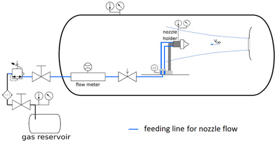
Figure 12.
Schematics of test-bench and feed system.
The main subcomponents of interest for the vacuum wind tunnel are a test chamber (or experimental room), evacuation units activated for performance tests under near-vacuum conditions, a fan/driving motor for the generation of the conical free-stream, and a pre-chamber [11]. In addition, the test chamber hosts a background-oriented schlieren (BOS) optical system for the flow visualisation [36], which provides qualitative comparisons of the flow field of the nozzle jets. The evacuation units allow the generation of near-vacuum conditions (∼7 kPa), while the radial fan provides low-subsonic free-stream velocities (up to ∼100 m/s) [37]. In Figure 13, the version of the setup adopted for the experimental activities is available. It is a pressure chamber hosting interchangeable nozzle models (additively manufactured with polymeric resins), mounted on an aluminium structure that slides with an axial 1-DOF, thus allowing force measurements through an S-shaped load cell mounted on the breadboard (see also Figure 12). Previous structural analyses proved that this configuration can resist any deformation under the bending loads considered, as well as accurate measurements to correct any influence of friction, pre-loads on the cell, and disturbances introduced by the pressurised flexible tubes under various ambient pressure conditions. The setup includes an aluminium body-extension too, which differs from the CFD simulations in favour of an aspect ratio () closer to real cases of interest. Additional details about the limits of comparability of results between experiments and CFD are provided in Section 6. The body-extension is connected to the pressure chamber through 3D-printed interfaces and presents pressure probes that could be adopted to measure the local pressure for the evaluation of the pressure coefficient. More details about the test facility, characteristics of the sensors, and test procedures are provided in previous publications by the TUD research group [10,11].
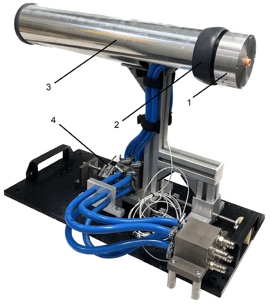
Figure 13.
Picture of the final setup: (1) pressure chamber and nozzle model, (2) chamber/body interface or support ring, (3) external body-extension, (4) S-shaped load cell.
5.3. Validation Process
The validation process is based on a comparison between the numerical results in Table 8 and Table 9 and the experimental values obtained during the test campaign [11] (refer to Section 5.2 for further details). The experimental results, and the performance gaps with the values obtained through the CFD simulations, are reported in Table 15.
Table 15.
Validation of performance, comparison at design point (PRF-OD) and at sea-level standard (PRF-SLS) between CFD and experimental data. More details (e.g., sensors accuracy, performance calculation) are available in previous publications by the authors [10,11].
A very good agreement is found for the performance of the AN and ED at the design point (gap between and ). The other simulations on ANCs return a 3–5% performance gap with respect to the experimental results for most of the cases, which is assumed as satisfying for the purposes of this study. One exception is the ED nozzle under SLS conditions: the RANS equations underestimated the performance; apparently the wake-evacuation effects generated at the pintle (aspiration drag) compromise the quality of the results (c.a lower thrust). A first analysis suggests that the influence of the small vortexes, which induce aspiration drag under SLS conditions, is not negligible for the ED nozzle. A similar phenomenon affected the DB nozzle, in this case by over-estimating the performance is SLS still within an acceptable margin (higher experimental losses, ca. +5%). However, a 3–5% performance gap poses a limit to the comparability of models based on RANS equations with the experimental results, thus suggesting the adoption of different models that include small vortexes and unsteady contributions (further discussed in Section 7). A separate discussion involves the RAO-bell nozzle: under SLS conditions, the design choice of a smoother throat angle for the CFD geometry determined lower losses due to over-expansion than for the nozzle adopted during the experiments.
The latter experiences a stronger re-compression at the wall, thus justifying the ca. +12% on thrust. However, this is not directly addressable to the numerical models, but rather to limitations that occurred during the experimental campaign. This is still considered acceptable, as the main focus of this study is actually more on the effectiveness of altitude compensation of ANCs in subsonic free-streams. In this sense, a more conservative approach for the performance comparison between ANCs and conventional nozzles at SLS is assumed, as a 10% safety margin on effective performance gains has to be accounted (refer to Section 6.1).
The final validation step is the qualitative visual comparison between the BOS pictures and the density gradient images from CFD post-processing. For all cases, it results in an excellent match between the flow topologies: an example of qualitative comparison between CFD post-processing (see Figure 14a) and correspondent BOS picture (experimental, see Figure 14b) is provided for the ED nozzle at its design point. In this case, the comparison yields a high correspondence between the type of operating mode, the extent of the viscous recirculation region, the length of the first shock cell, and general properties of reflected shock waves.
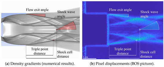
Figure 14.
Qualitative comparison of flow topology for ED nozzle at design point ().
6. Discussion of Results
A qualitative and quantitative discussion of results for the numerical simulations is offered in this section. This includes nozzle performance and aerodynamic performance of the extended body while invested by subsonic free-streams, together with a discussion dedicated to comparability with empirical models for prediction of jet penetration in closure.
6.1. Discussion on Nozzle Performance
The first discussion includes a more detailed comparison of the nozzle performance at sea-level standard between the models designed for near-vacuum (ANCs) and the nozzle designed for near-SLS operations (RAO-bell). An overview is provided in Table 16.
Table 16.
Performance comparison under SLS conditions between advanced nozzles () and RAO-bell nozzle ().
The RAO-bell nozzle behaved in high over-expansion, generating a Mach disk close to the exit section that reduces the nozzle efficiency under SLS conditions. On the contrary, the AN and DB nozzles preserved a relatively high thrust at SLS despite their higher expansion ratios, with the aerospike outperforming with a +6.33% on thrust. This is a lower value than the 15.0% indicated in the literature [9,18,22,23], as the latter refers to the performance gains achievable at design point by aerospike engines designed at a high expansion ratio. As expected, the ED nozzle underperformed the RAO-bell (ca. −28% on thrust), thus confirming a scarce altitude compensation capability due to wake-evacuation effects [29]. Interestingly, the DB nozzle achieved a thrust increment similar to the aerospike, but at a lower specific impulse and thrust coefficient. This was due to the adaptation of the throat area for the AN, ca. 4% smaller (minor ) than the value in Table 1. This was needed for comparability of results between different ANCs operating at the same on design. Indeed, the same exit Mach number was verified within a ±1.0% margin (refer to Table 8). In addition, the DB nozzle experiences additional losses induced by the aspiration drag during low-altitude operations [38]. The combination of these factors determines an overall higher efficiency for the aerospike and comparable thrust gains with respect to the DB nozzle under SLS conditions.
A performance comparison at sea level, between static-fire (PRF-SLS) and retro-flow (RFL) simulations, is offered in Table 17. As described in Section 4.1, the presence of a counteracting free-stream influences the nozzle performance. This is due to the fact that the local static pressure within the recirculation region ( or dead air pressure at nozzle exit) is lower that the ambient pressure in the absence of counter-flow (). The results in Table 17 show increments between 1 and 2% of the for all the nozzles. The actual performance increments depend on a combination of two factors: the lower static pressure in the recirculation zone (, refer to Section 4.1) and the interaction between aerodynamic jet boundaries and the counter-flow of ANCs (influence over ) [8]. A general result is that the estimation of results is more accurate when referred to the dead air pressure (), coherently with the performance increments. However, in the absence of good estimation of local within the recirculation region, the asymptotic free-stream pressure () still works better than ambient pressure () for estimating the (refer to Table 10). Interestingly, the sensitivity of the DB nozzle to changes in effective appears lower than for other nozzles; on the contrary, the effect on thrust doubles for the ED nozzle. In the first case, the core nozzle of the DB is designed for sea-level and operates close to the optimum expansion, therefore it is less sensitive to variations of at sea level. In contrast, the ED nozzle presents the highest expansion ratio (refer to Section 3.1), thus higher sensitivity to changes in .
Table 17.
Numerical results on variation of nozzles performance between static-fire and retro-flow configurations at SLS (, ).
6.2. Discussion on Aerodynamic Performance
The following section focuses on the aerodynamics of an extended body being invested by a subsonic stream, and the effects of retro-propulsion. The analysis focuses only on the impact on drag, for null Angle of Attack (AOA), absence of thrust-vectoring, and by neglecting the effects of wake drag (refer to Section 3.1). These limitations are sufficient to proceed with the evaluation of the normalised jet penetration and assessment of the role of pressure drag at the base plate and viscous-drag over the extended body. The downside is that the current models are not directly representative of a real case because of the absence of wake drag.
The simulations performed in counter-flow returned a Reynolds number of the free-stream (, transient-flow) approximately one order of magnitude lower than those experienced during a landing manoeuvre (fully developed turbulent-flow). It should be noted that the point of flow separation changes substantially between a transient-flow and a turbulent-flow, but the sharp edge at the base plate ensures that the separation is fixed, regardless of the Reynolds number of the free-stream. Although the vortex structures should be smaller compared to a sub-scaled experiment’s, the comprehensive structure of the nozzle-jet/free-stream interaction (AI area) would still be dominated by the of the free-stream against the nozzle jet. Coherently with Nonaka et al. [16], despite the being an order of magnitude lower than the real case, the flow topology of the AI region is qualitatively comparable with that around the vehicle in a real case. This is true as long as the flow separation occurs at the edge of the base plate (verified numerically and experimentally).
The simulations in retro-flow configurations assess the impact of subsonic retro-propulsion (SubRP) on the total drag coefficient () and each of its contributions ( and , refer to Section 2). To do so, the data provided in Table 11 and Table 12 are re-elaborated in agreement with Equation (2) and presented in Figure 15. The latter shows that thrust-induced drag () is the predominant contribution to total drag during subsonic retro-propulsion. This is confirmed by the result in Figure 16, where the direct proportionality of the increment of total drag with is highlighted. Such a result is not trivial, as it is a consequence of a minor impact of the thrust-induced drag over the aerodynamic drag; indeed, the latter results independent from the nozzle type, implying that the total drag is directly proportional to . A similar result cannot be found for the momentum ratio between the nozzle jet and free-stream ( multiplied by , refer to Section 2). This result confirms that substitutes the momentum ratio as the correct parameter to consider if the pressure contribution in the Equation (7) cannot be neglected; this is the case for over-expanded conventional nozzles and altitude compensating nozzles.
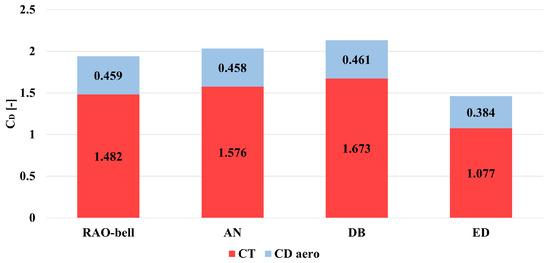
Figure 15.
Numerical results on total drag coefficient () of the extended body in retro-flow scenario (, uniform free-stream at ).
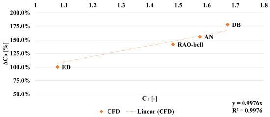
Figure 16.
Direct proportionality between aerodynamics thrust coefficient () and increments of total pressure drag () of the extended body in retro-flow scenario (, uniform free-stream at ).
It should be noted that no wake drag contribution is included in this analysis; however, this does not affect the validity of the observation because the free-stream at the side-walls presents an air-speed value coincident with the asymptotic value (, refer to Table 12), independent of the nozzle type. As a consequence, the term of wake drag constitutes a constant contribution to the total drag; thus, it does not affect the direct proportionality of with the thrust-induced drag.
Additional insights are obtained from examining the increment of and decrement of with respect to the counter-flow case (see Figure 17). The decrement of aerodynamic drag is large (). However, it is smaller than during any re-entry burn manoeuvre at high altitudes (supersonic retro-propulsion, or SRP), during which the aerodynamic drag coefficient typically falls by one order of magnitude and in some cases is even negative (suction) [7,8]. One interesting result is that the ANCs achieve a higher total drag without a large impact on the reduction in aerodynamic drag with respect to the conventional nozzle. Indeed, the reduction in results always between 40 and 43%, independently from the nozzle type (with the exception of the ED nozzle).
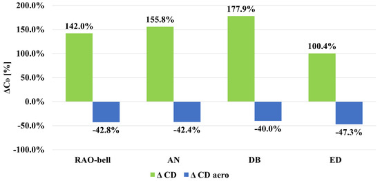
Figure 17.
Numerical results on increment of total drag coefficient () and decrement of aerodynamic drag coefficient () of the extended body in retro-flow scenario (, uniform free-stream at ).
The ED nozzle constitutes an exception to this, as it provides the largest reduction in aerodynamic drag (despite having the lowest ). This nozzle offers the highest form-factor (), and there is evidence of correlation between the pressure coefficient at the base plate (refer to Table 12) and the ambient pressure ratio () times the form-factor. This is deduced from Figure 18, where such correlation is highlighted. As the pressure at the base plate estimates the dead air pressure value () within the recirculation region, it might be of interest to investigate this aspect further. Indeed, the dead air pressure has a direct impact over the aerodynamic drag at the base plate and effective of the nozzles. However, a clearer statement is unobtainable at this stage, because the nozzles in Figure 18 operate at a different conditions. To demonstrate a direct proportionality, a dedicated campaign should be performed between nozzles operating at the same momentum flux ratio between jets and free-stream, but offering different combinations of ambient pressure ratios and form-factors.
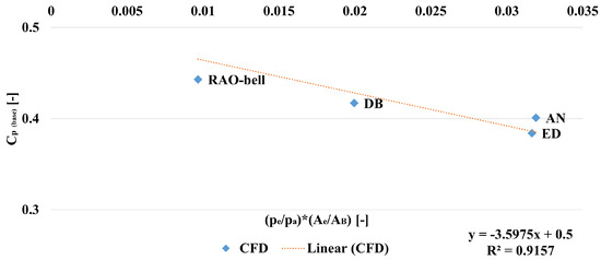
Figure 18.
Direct proportionality between APR () times the form-factor () and pressure coefficient at the base plate () in retro-flow scenario (, uniform free-stream at ).
6.3. Discussion on Jet Penetration
To better predict the physics of retro-propulsion for lander applications, one successful approach was introduced to predict the flow topology of the Aerodynamics Interference (AI) region from its scaling parameters (e.g., , , ). A similar methodology is adopted also to estimate the normalised jet penetration distance () of retrorocket exhausts into subsonic counter-flows [14,15]. In this study, such an approach was pursued on advanced nozzles in retro-flow configurations, starting from data provided in Table 12. The latter was re-adapted in Table 18 to be verified through the empirical formulation by Jarvinen et al. [15] (refer to Equation (1)). The methodology requires for each nozzle to be known: the momentum flux ratio () and the temperature ratio between chamber and exit (); additionally, the aerodynamics thrust coefficient () is provided. The results for different nozzle type are offered in Figure 19.
Table 18.
Scaling parameters for the Aerodynamics Interference (AI) region ( m/s uniform, ambient conditions at SLS).
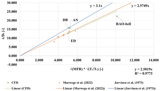
Figure 19.
Normalised jet penetration distance () for advanced and bell-shaped nozzles in retro-flow scenario (, uniform free-stream at ) and comparison with reference values available in the literature [14,15].
The first observation is that the advanced nozzles in this study perfectly fall within the interval defined by the data available in the literature. In particular, an important consequence of this result is that ANCs are compatible with the empirical formulation in Equation (1), thus the jet penetration distance can be estimated in the case of altitude compensating nozzles invested by subsonic counter-flows with a satisfying level of confidence. Such a result is not trivial, as the mechanism behind the altitude compensation plays a significant role on the flow topology of the AI region. Nevertheless, jet penetration distance can be estimated by simply knowing the momentum flux ratio between nozzle jet and free-stream and the temperature ratio between the chamber and nozzle exit section. For the specific case of the RAO-bell nozzle, the jet penetration distance falls out from the experimental interval (ca. 15% shorter). However, this margin is relatively small (ca. 50 mm) by considering the smaller of RAO-bell nozzle. Future studies adopting alternative numerical models (e.g., Unsteady-RANS or Large-Eddy Simulations) could investigate this phenomenon with a higher resolution.
7. Limitations and Outlook
This section reports the limitations of the models, suggestions for improvements, and future activities. The validation process is limited by the absence of dedicated tests for the models in retro-flow configurations (performance cases are validated with experiments, instead). This comes as the test-bench adopted during the experimental campaign in TUD supports only conical counter-flows (instead of uniform), which a priori present a different flow topology over the extended body (for details, refer to Section 5.2 and previous publications [10,11]). Nevertheless, validation of results through empirical formulations and comparison with reference values available in the literature (refer to Section 6.3) ensure a realistic representation of the (time-averaged) flow topology of the AI regions.
In general, the numerical models defined for this study could benefit from adopting alternative numerical models to better capture the contribution of smaller vortexes and unsteadiness of the AI region (i.e., Large-Eddy Simulations and Unsteady-RANS), which is usually neglected when adopting models based on RANS equations (time-averaged solution). Moreover, the creation of large recirculation areas is visible for both the truncated AN and the ED nozzles. This area can have a significant influence on the base pressure. Alternative turbulence models such as RNG are well suited for these kind of recirculating flows: for the latter, it has been demonstrated that this still holds true for supersonic separated flows [39], giving better results than SST in predicting the base pressure [40]. However, other research has shown that the SST turbulence model allows for a better capturing of the shock structure of the flow compared to the RNG [41] as well as superior performance for external supersonic and hypersonic flows [42,43]. A separate investigation would be needed to examine to what extent errors in the flow structure or resolution of the base pressure would contribute to the overall results. A sensitivity analysis, comparing various turbulence models and their effect on the accuracy of the specific flow regimes, as well as on the general results, could be employed to gain more insight into the best choice of turbulence models for this specific case. Furthermore, the use of Unsteady-RANS simulations makes it possible to study altitude compensation considering a time-increasing ambient pressure, thus more realistically resembling a powered vertical landing manoeuvre (i.e., landing burn, performed by the reusable main-stages of Falcon 9 and Falcon Heavy).
Additionally, the investigation might benefit from including non-null angles of attack and by enlarging the range of momentum flux ratios to be investigated. This study proves that the mechanism of altitude compensation of ANCs is compatible with subsonic counter-flows (). Moreover, it suggests that an annular aerospike achieves such performance gains with higher efficiency and smaller volumetric encumbrance of a DB nozzle (35% shorter length). Therefore, future activities by the research group include a numerical study of a VTVL-RLV concept [44] comparing a conventional octa-web configuration with a high expansion ratio aerospike. In particular, the choice falls on the latter because the expansion ratio increases (in theory) up to the diameter of the base plate, thus maximising the performance during vacuum operations. At the same time, it still offers altitude compensation capabilities during descent and under sea-level conditions; however, the engine design and integration would be more difficult than for a dual-bell nozzle, which still offers an interesting compromise between performance gains and architecture complexity.
8. Conclusions
A numerical study was conducted on advanced nozzle concepts for retro-propulsion applications, including a comparison with a conventional bell-shaped nozzle. This study demonstrated that the advanced nozzles (annular-aerospike, dual-bell, and expansion-deflection nozzles) conserve their altitude compensation capabilities while being invested by subsonic counter-flows. The interaction between the nozzle jet and the free-stream was discussed and its impact on propulsion and aerodynamic performance were analysed. Annular-aerospike and dual-bell nozzles performed better than the conventional nozzle (+6% thrust) under sea-level conditions, despite their higher expansion ratio. This is because the dual-bell and the aerospike recover the over-expansion losses through the mechanism of altitude compensation. For low Mach numbers (<0.2) of the counter-flow, the thrust-induced drag is the major contributor to the total drag, whose increments show direct proportionality with the aerodynamics thrust coefficient (). The average pressure within the recirculation region (lower than ambient pressure) increases the nozzle pressure ratio. Consequently, all nozzles performed better (+1% thrust, at null angles of attack) than in the absence of counter-flows. The performance validation proved good agreement between the CFD and experiments (except the wake-evacuation effects for the expansion-deflection nozzle). This was achieved with numerical models based on RANS equations and the Shear-Stress Transport (SST) turbulence model, which offer an interesting compromise between high-fidelity results and low computational costs. Nevertheless, alternative numerical models are advisable for future studies to better capture the effects of smaller vortexes and to study the stability of the recirculation region. The numerical models proved advanced nozzles to be compatible with empirical formulations for predicting jet penetration distance into subsonic counter-flows. Such a conclusion is not trivial, as the mechanism behind the altitude compensation influences both the flow topology and radial extension of the recirculation region.
Author Contributions
Conceptualization, G.S. and M.P. (Martin Propst); methodology, M.P. (Martin Propst) and G.S.; numerical simulations, M.G., J.P. and F.W.; experimental validation, G.S., M.P. (Marco Portolani), J.S.-K. and T.H.; formal analysis, M.G. and G.S.; data curation, G.S.; writing—original draft preparation, G.S.; writing—review and editing, M.P. (Martin Propst), J.P. and C.B.; visualization, G.S. and M.G.; supervision, D.B., D.P., A.F., M.T. and C.B.; project management, T.H. and J.P.; project coordination, C.B.; funding acquisition, C.B. All authors have read and agreed to the published version of the manuscript.
Funding
The project leading to this application has received funding from the European Union’s Horizon 2020 research and innovation program under the Marie Skłodowska-Curie grant agreement No. 860956.
Institutional Review Board Statement
Not applicable.
Informed Consent Statement
Not applicable.
Data Availability Statement
The data supporting reported results can be found in publicly archived datasets generated during the study, available upon request to the corresponding authors at the following repository: https://gitlab.hrz.tu-chemnitz.de/gisc630c--tu-dresden.de/tud-database (accessed on 18 December 2024).
Acknowledgments
Special thanks to Alessia Gloder for managing the ASCenSIon project during the first years of activity. Furthermore, thanks to Adheena Gana Joseph for supporting the experimental activities with BOS visualisation and for her efforts to project management, together with Maximilian Buchholz for their ideas and support during the manufacturing and integration of the test-bench. Final thanks to Jürgen Frey for their technical support to operate the vacuum wind tunnel facility.
Conflicts of Interest
The authors declare no conflict of interest.
References
- Jefferies International LLC. Report on Falcon 9. Technical Report, SpaceNews.com, 2016. Available online: https://spacenews.com/spacexs-reusable-falcon-9-what-are-the-real-cost-savings-for-customers (accessed on 17 September 2021).
- Jones, H.W. The Recent Large Reduction in Space Launch Cost. In Proceedings of the 48th International Conference on Environmental Systems, Albuquerque, NM, USA, 8–12 July 2018. ICES-2018-81. [Google Scholar]
- OurWorldInData.org. Cost of Space Launches to low Earth Orbit. Data Source: CSIS Aerospace Security Project (2022). 2022. Available online: https://ourworldindata.org/grapher/cost-space-launches-low-earth-orbit (accessed on 9 March 2024).
- Vernacchia, M.T.; Mathesius, K.J. Strategies for Reuse of Launch Vehicle First Stages. In Proceedings of the 69th International Astronautical Congress 2018, Bremen, Germany, 1–5 October 2018. Number IAC-18-D2.4.3. [Google Scholar]
- Stappert, S.; Wilken, J.; Bussler, L.; Sippel, M. A Systematic Assessment and Comparison of Reusable First Stage Return Options. In Proceedings of the 70th International Astronautical Congress (IAC), Washington, DC, USA, 21–25 October 2019. [Google Scholar]
- OurWorldInData.org. Annual Number of Objects launched into Space. 2024. Data Source: United Nations Office for Outer Space Affairs (2024). Available online: https://ourworldindata.org/grapher/yearly-number-of-objects-launched-into-outer-space (accessed on 9 March 2024).
- Ecker, T.; Karl, S.; Dumont, E.; Stappert, S.; Krause, D. Numerical Study on the Thermal Loads During a Supersonic Rocket Retropropulsion Maneuver. J. Spacecr. Rocket. 2020, 57, 131–146. [Google Scholar] [CrossRef]
- Scarlatella, G.; Tajmar, M.; Bach, C. Advanced Nozzle Concepts in retro-propulsion applications for Reusable Launch Vehicle recovery: A case study. In Proceedings of the 72nd International Astronautical Congress (IAC), Dubai, United Arab Emirates, 25–29 October 2021. [Google Scholar]
- Hagemann, G.; Immich, H.; Nguyen, T.V.; Dumnov, G.E. Advanced Rocket Nozzles. J. Propuls. Power 1998, 14, 620–634. [Google Scholar] [CrossRef]
- Scarlatella, G.; Sieder-Katzmann, J.; Roßberg, F.; Weber, F.; Mancera, C.T.; Bianchi, D.; Tajmar, M.; Bach, C. Design and Development of a Cold-Flow Test-Bench for Study of Advanced Nozzles in Subsonic Counter-Flows. Aerotec. Missili Spaz. 2022, 101, 201–213. [Google Scholar] [CrossRef]
- Scarlatella, G.; Heutling, T.; Sieder-Katzmann, J.; Weber, F.; Portolani, M.; Garutti, M.; Bianchi, D.; Ferrero, A.; Pastrone, D.G.; Tajmar, M.; et al. Cold-Gas Experiments on Advanced Nozzles in Subsonic Counter-Flows. In Proceedings of the Aerospace Europe Conference 2023—10th EUCASS—9th CEAS, Lausanne, Switzerland, 9–13 July 2023. [Google Scholar]
- Korzun, A.M.; Cassel, L.A. Scaling and Similitude in Single Nozzle Supersonic Retropropulsion Aerodynamics Interference. In Proceedings of the AIAA Scitech 2020 Forum, Orlando, FL, USA, 6–10 January 2020. [Google Scholar] [CrossRef]
- Bykerk, T.; Karl, S. Preparatory CFD Studies for Subsonic Analyses of a Reusable First Stage Launcher during Landing within theRETPRO Project. In Proceedings of the Aerospace Europe Conference 2023—10th EUCASS—9th CEAS, Lausanne, Switzerland, 9–13 July 2023. [Google Scholar]
- Marwege, A.; Hantz, C.; Kirchheck, D.; Klevanski, J.; Vos, J.; Laureti, M.; Karl, S.; Gulhan, A. Aerodynamic Phenomena of Retro Propulsion Descent and Landing Configurations. In Proceedings of the 2nd International Conference on Flight Vehicles, Aerothermodynamics and Re-Entry Missions & Engineering (FAR), Heilbronn, Germany, 19–23 June 2022. [Google Scholar] [CrossRef]
- Jarvinen, P.O.; Hill, J.A.F. Penetration of retrorocket exhausts into subsonic counterflows. J. Spacecr. Rocket. 1973, 10, 85–86. [Google Scholar] [CrossRef]
- Nonaka, S.; Nishida, H.; Kato, H.; Ogawa, H.; Inatani, Y. Vertical Landing Aerodynamics of Reusable Rocket Vehicle. Trans. Jpn. Soc. Aeronaut. Space Sci. Aerosp. Technol. Jpn. 2012, 10, 1–4. [Google Scholar] [CrossRef]
- Gutsche, K.; Marwege, A.; Gülhan, A. Similarity and Key Parameters of Retropropulsion Assisted Deceleration in Hypersonic Wind Tunnels. J. Spacecr. Rocket. 2021, 58, 984–996. [Google Scholar] [CrossRef]
- Sutton, G.P.; Biblarz, O. Chapter 3: “Nozzle Theory and Thermodynamic Relations”. In Rocket Propulsion Elements; Wiley: Hoboken, NJ, USA, 2017; pp. 46, 50, 62–63, 72. Available online: https://www.ebook.de/de/product/23826026/george_p_sutton_oscar_biblarz_rocket_propulsion_elements_9_e.html (accessed on 18 December 2024).
- Marwege, A.; Gülhan, A. Unsteady Aerodynamics of the Retropropulsion Reentry Burn of Vertically Landing Launchers. J. Spacecr. Rocket. 2023, 60, 1939–1953. [Google Scholar] [CrossRef]
- Marwege, A.; Gülhan, A. Aerodynamic Characteristics of the Retro Propulsion Landing Burn of Vertically Landing Launchers. Res. Sq. 2023; preprint. [Google Scholar] [CrossRef]
- Jarvinen, P.O.; Adams, R.H. The aerodynamic characteristics of large angled cones with retrorockets. In Techreport Contract No. NAS 7-576, National Aeronautics and Space Administration Liquid Rocket Research and Technology Code RPL, Washington, D.C., 1970; MITHRAS, a Division of Sanders Associates, Inc.: Cambridge, MA, USA, 1970. [Google Scholar]
- Onofri, M.; Calabro, M.; Hagemann, G.; Immich, H.; Sacher, P.; Nasuti, F.; Reijasse, P. Plug nozzles: Summary of flow features and engine performance—Overview of RTO/AVT WG 10 subgroup 1. In Proceedings of the 40th AIAA Aerospace Sciences Meeting & Exhibit, Reno, NV, USA, 14–17 January 2002. [Google Scholar] [CrossRef][Green Version]
- Bach, C.; Schöngarth, S.; Bust, B.; Propst, M.; Sieder-Katzmann, J.; Tajmar, M. How to steer an aerospike. In Proceedings of the 69th International Astronautical Congress (IAC), Bremen, Germany, 1–5 October 2018; Available online: https://www.researchgate.net/publication/328145907_How_to_steer_an_aerospike (accessed on 13 September 2024).
- Ghosh, D.; Gunasekaran, H. Large Eddy Simulation of Aerospike Nozzle assisted Supersonic Retro-Propulsion. In Proceedings of the AIAA Aviation 2021 forum. American Institute of Aeronautics and Astronautics, Virtual Event, 2–6 August 2021. [Google Scholar] [CrossRef]
- Sutton, G.P.; Biblarz, O. Rocket Propulsion Elements, 9th ed.; Number 14 in 5; Wiley: Hoboken, NJ, USA, 2017; Available online: https://www.ebook.de/de/product/23826026/george_p_sutton_oscar_biblarz_rocket_propulsion_elements_9_e.html (accessed on 18 December 2024).
- Propst, M.; Sieder-Katzmann, J.; Abel, J.; Schwarzer-Fischer, E.; Scheithauer, U.; Tajmar, M.; Bach, C. Influence of manufacturing accuracy on the performance characteristics of miniaturized ceramic cold-gas thrusters. In Proceedings of the Space Propulsion Conference, Estoril, Portugal, 9–13 May 2022. [Google Scholar]
- Lee, C.C. Technical Note—Fortran Programs For Plug Nozzle Design; Technical Report; Scientific Research Laboratories, Brown Engineering Company, Inc.: Reading, PA, USA, 1963; Available online: https://archive.org/details/nasa_techdoc_19630012259/ (accessed on 27 May 2024).
- Génin, C.; Schneider, D.; Stark, R. Dual-Bell Nozzle Design. In Notes on Numerical Fluid Mechanics and Multidisciplinary Design; Springer International Publishing: Cham, Switzerland, 2020; pp. 395–406. [Google Scholar] [CrossRef]
- Taylor, N.V. Simulating cross altitude performance of expansion deflection nozzles. In Proceedings of the 57th International Astronautical Congress, Valencia, CA, USA, 2–6 October 2006; Volume 14, pp. 620–634. [Google Scholar] [CrossRef]
- Mancera, C.T. Numerical Simulations of Advanced Rocket Nozzles Forretro-Propulsion in Subsonic Counter-Flows. Master’s Thesis, Technische Universität Dresden, Dresden, Germany, 2021. [Google Scholar]
- Ansys©, Inc. Ansys Fluent 12.0 User’s Guide, Release 12.0© Ansys, Inc. 2009-01-29 ed.; 2009; Available online: https://www.afs.enea.it/project/neptunius/docs/fluent/html/ug/main_pre.htm (accessed on 11 March 2024).
- Propst, M.; Sieder-Katzmann, J.; Stark, R.; Schneider, D.; General, S.; Tajmar, M.; Bach, C. Active—Optimisation of a Fluidic Thrust Vector Control on Aerospike Nozzles. In Proceedings of the Space Propulsion Conference, Virtual, 17–19 March 2021. [Google Scholar]
- Tu, J.; Yeoh, G.H.; Liu, C. Computational Fluid Dynamics: A Practical Approach, 3rd ed.; Butterworth-Heinemann: Oxford, UK, 2018. [Google Scholar]
- Menter, F. Zonal Two Equation k-w Turbulence Models For Aerodynamic Flows. In Proceedings of the 23rd Fluid Dynamics, Plasmadynamics, and Lasers Conference. American Institute of Aeronautics and Astronautics, Orlando, FL, USA, 6–9 July 1993. [Google Scholar] [CrossRef]
- Stark, R. Flow Separation in Rocket Nozzles, a Simple Criteria. In Proceedings of the 41st AIAA/ASME/SAE/ASEE Joint Propulsion Conference & Exhibit, Tucson, AZ, USA, 10–13 July 2005. [Google Scholar] [CrossRef]
- Settles, G.S. Toepler’s Schlieren Technique. In Schlieren and Shadowgraph Techniques; Springer: Berlin/Heidelberg, Germany, 2001; pp. 39–75. [Google Scholar] [CrossRef]
- Leonhardsberger, M.; Strohmer, P. Internal Report: Vacuum Wind Tunnel Facility; Technical Report; Technische Universität Dresden: Dresden, Germany, 2004. [Google Scholar]
- Liu, Y.; Li, P. Analysis of the Aspiration Drag in Dual-Bell Nozzles. Int. J. Aeronaut. Space Sci. 2022, 24, 467–474. [Google Scholar] [CrossRef]
- Papp, J.; Ghia, K. Application of the RNG turbulence model to the simulation of axisymmetric supersonic separated base flows. In Proceedings of the 39th Aerospace Sciences Meeting and Exhibit. American Institute of Aeronautics and Astronautics, Reno, NV, USA, 8–11 January 2001. [Google Scholar] [CrossRef]
- Dharavath, M.; Sinha, P.K.; Chakraborty, D. Simulation of supersonic base flow: Effect of computational grid and turbulence model. Proc. Inst. Mech. Eng. Part G J. Aerosp. Eng. 2009, 224, 311–319. [Google Scholar] [CrossRef]
- Raghavendra Rao, M.; Amba Prasad Rao, G.; Charyulu, B.; Singh, H. Numerical studies and validation of combustor and annular isolator interactions of hydrocarbon based axisymmetric dual combustion ramjet. Aerosp. Sci. Technol. 2020, 106, 106185. [Google Scholar] [CrossRef]
- López, D.; Domínguez, D.; Gonzalo, J. Impact of turbulence modelling on external supersonic flow field simulations in rocket aerodynamics. Int. J. Comput. Fluid Dyn. 2013, 27, 332–341. [Google Scholar] [CrossRef]
- Javad Ameri, M.; Reza Heidari, M.; Nowruzi, H.; Najafi, A. Analysis of Different Turbulence Models in Simulation of Hypersonic Flow in the Wind Tunnel. Am. J. Mech. Eng. 2019, 7, 172–180. [Google Scholar]
- Scarlatella, G.; Tajmar, M.; Bach, C.; Guadagnini, J.; de Zaiacomo, G.; Panicciá, L.; Pastrone, D.G. Assessment of Mission Capabilities of a Reusable Heavy-lift Launch Vehicle Concept with Aerospike Engine. In Proceedings of the AIAA Scitech 2024 Forum, American Institute of Aeronautics and Astronautics, Orlando, FL, USA, 8–12 January 2024. [Google Scholar] [CrossRef]
Disclaimer/Publisher’s Note: The statements, opinions and data contained in all publications are solely those of the individual author(s) and contributor(s) and not of MDPI and/or the editor(s). MDPI and/or the editor(s) disclaim responsibility for any injury to people or property resulting from any ideas, methods, instructions or products referred to in the content. |
© 2025 by the authors. Licensee MDPI, Basel, Switzerland. This article is an open access article distributed under the terms and conditions of the Creative Commons Attribution (CC BY) license (https://creativecommons.org/licenses/by/4.0/).