Spin Period Evolution of Decommissioned GLONASS Satellites

Abstract

Light curve analysis of defunct satellites is critical for characterizing their rotational motion. An accurate understanding of this aspect will benefit active debris removal and on-orbit servicing missions as part of the solution to the space debris issue. In this study, we explored the attitude behavior of inactive GLONASS satellites, specifically a repeating pattern observed in their spin period evolution. We utilized a large amount of data available in the light curve database maintained by the Astronomical Institute of the University of Bern (AIUB). The morphology of the inactive GLONASS light curves typically features four peaks in two pairs and is presumably attributed to the presence of four evenly distributed thermal control flaps or radiators on the satellite bus. The analysis of the periods extracted from the light curves shows that nearly all of the inactive GLONASS satellites are rotating and exhibit a periodic oscillating pattern in their spin period evolution with an increasing or decreasing secular trend. Through modeling and simulation, we found that the periodic pattern is likely a result of canted solar panels that provide an asymmetry in the satellite model and enable a wind wheel or fan-like mechanism to operate. The secular trend is a consequence of differing values of the specular reflection coefficients of the front and back sides of the solar panels. Assuming an empirical model describing the spin period evolution of 18 selected objects, we found significant variations in the average spin period and amplitude of the oscillations, which range from 8.11 s to 469.58 s and 1.10 s to 513.24 s, respectively. However, the average oscillation period remains relatively constant at around 1 year. Notably, the average spin period correlates well with the average amplitude. The empirical model can be used to extrapolate the spin period in the future, assuming that the oscillating pattern is preserved and roughly shows a linear trend.

1. Introduction

Modern human civilization depends on space technology. Orbiting spacecrafts are now vital as communications links, navigation beacons, scientific investigation platforms, and providers of remote sensing data for weather, climate, land use, and national security purposes. However, as the number of spacecrafts increase, the number of undesirable consequences related to space activities also escalates. Space debris is any artificial object in orbit without a useful function, including non-functional spacecraft, spent rocket bodies, mission-related objects, and breakup fragments. The combination of speed and lack of control makes space debris a threat to space activity. To protect the space environment, mitigation and remediation measures have been suggested in the past. Remediation would be performed by moving selected debris to a desired orbit (of little operational value) or bringing it back to Earth through so-called active debris removal (ADR). Several methods have been proposed for carrying out ADR missions, for example, using a special satellite equipped with a robotic arm to capture a target and then dragging it into the atmosphere. For these missions, the knowledge of the attitude, motion, and spin period evolution of the object is essential. Ultimately, for space debris research, it is important to identify the mechanisms causing changes in the rotation of space objects. In particular, the indefinite increase in the spin rate might be a serious concern because centrifugal forces could cause spacecrafts to fall apart, creating further debris.

Light curves are passive optical measurements of space objects that show the variation in the observed object’s magnitude as a function of time and can be used to determine attitude states of space debris, including spin period [1,2,3] and spin axis orientation [4,5,6,7]. Recently, methods for attitude determination using spectral light curves were also proposed [8,9].

The Astronomical Institute of the University of Bern (AIUB) maintains a light curve database with more than 3000 light curves from 512 selected space objects [10]. In the database, the spin period evolution of some decommissioned GLONASS satellites reveals an interesting annual oscillating pattern [11]. Lee et al. [12] determined the spin axis of this type of satellite from photometric observations, but without analyzing the evolution. Studies on the spin period evolution have been conducted in the past, e.g., in [13,14,15], but not in the same orbit regime or on satellites equipped with retro-reflectors with more characterization possibilities [16,17,18]. Pontieu [19] reported a preliminary study of tumbling period evolutions for discarded third stages. Albuja et al. [20] used the Yarkovsky–O’Keefe–Radzievskii–Paddack (YORP) effect to simulate the interchange between increasing and decreasing rotational period. They found, based on [21], that solar radiation pressure leads to a complex, tumbling rotation, and they obtained an estimate of the evolution of angular velocity. In [22], the authors further hypothesize that there is a cyclical process: when the satellite begins to tumble due to YORP torque, it spins about the minimum moment of inertia, but at a certain stage, energy dissipation becomes an important factor and causes it to switch to a rotation about the maximum moment of inertia. Once a stable spin is reached, the YORP effect again becomes the major torque on the satellite, starting the cycle from the beginning. Benson et al. [23,24] analyzed aperiodic light curves of defunct GOES satellites covering several years to explore the cycle hypothesis, and they found them to be consistent with the suggested model. Earl [14] successfully simulated ECHOSTAR 2’s spin period variations considering canted solar panels with different orientations and different reflectivity for the front and back sides. He also noted from the characteristics of the light curves that, in addition to the solar panels, the highly reflective radiators of the satellite also produce bright specular flares.

In this paper, we want to study the spin period evolution of defunct GLONASS satellites based on the available light curves in the database and build on the knowledge of possible mechanisms identified in previous research. From the literature, we also see that other satellites show specific patterns with increasing and decreasing phases in the spin period evolution. However, a number of GLONASS satellites exhibit a very clear and regular evolution, which make them ideal candidates for this kind of study, assuming that the same underlying mechanism is responsible for these patterns.

The next section will describe the characteristics of GLONASS satellites, while in Section 3, the observed light curves and their specific features are presented. In Section 4, a group of GLONASS satellites with a quite regular spin evolution is selected, a model is proposed to describe the characteristic pattern, and statistical considerations are exposed. Finally, in Section 5, simulations based on a simple model are performed in an attempt to reproduce the evolution pattern.

2. GLONASS Satellites

GLONASS (Global’naya Navigatsionnaya Sputnikova Sistema) is the second group of satellite navigation systems in MEO after the GPS (Global Positioning System). Three generations of GLONASS satellites have been built and operated for nearly 40 years. The first generation consists of four types or blocks (I, IIa, IIb, and IIv). The second generation, GLONASS-M, was launched after 2003, and the third generation, GLONASS-K, was introduced in 2011. Only GLONASS IIv and GLONASS-M will be considered in this study. These two types of satellite share the same core structure, but GLONASS-M satellites are easily distinguished by the different placement of the solar panel rotation axis, and they no longer carry a magnetometer boom. They both employ a pressurized platform design and have a similar mass of roughly 1.4 tons, with a cylindrical structure with a length of about 3.5 m. GLONASS-M satellites have significantly larger solar arrays (32 m² instead of 25 m²). Heat dissipation is achieved through heat exchangers and four thermal control flaps, which are distributed evenly around the bus. The opening angle of these shutters can be varied and allows the adjustment of the internal temperature [25].

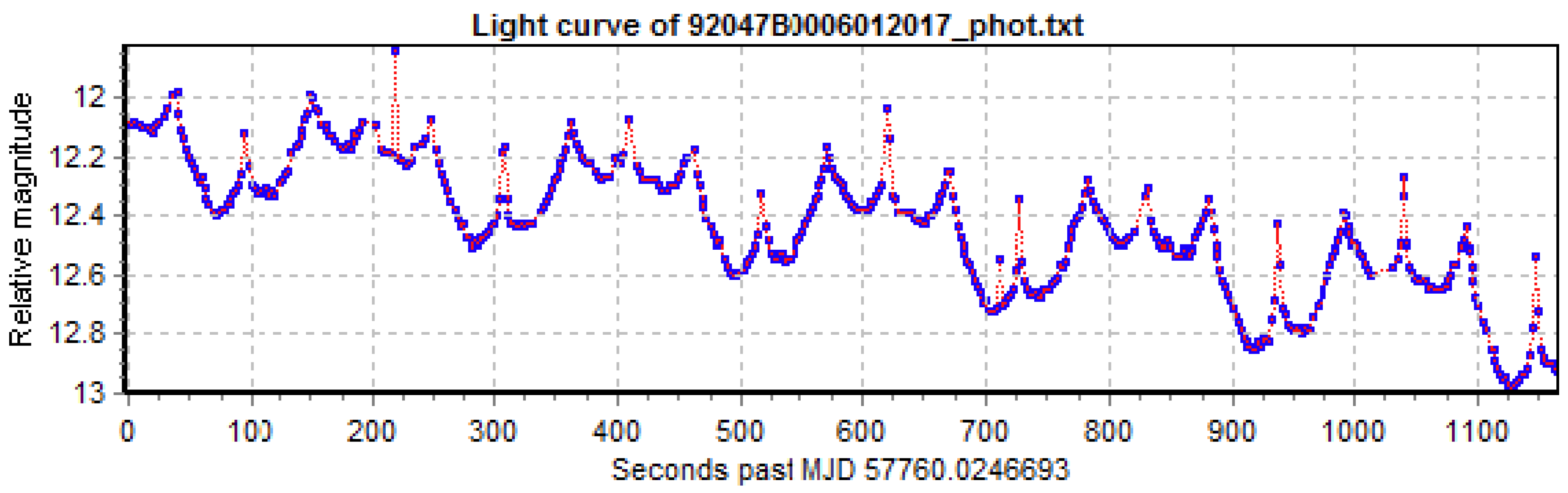
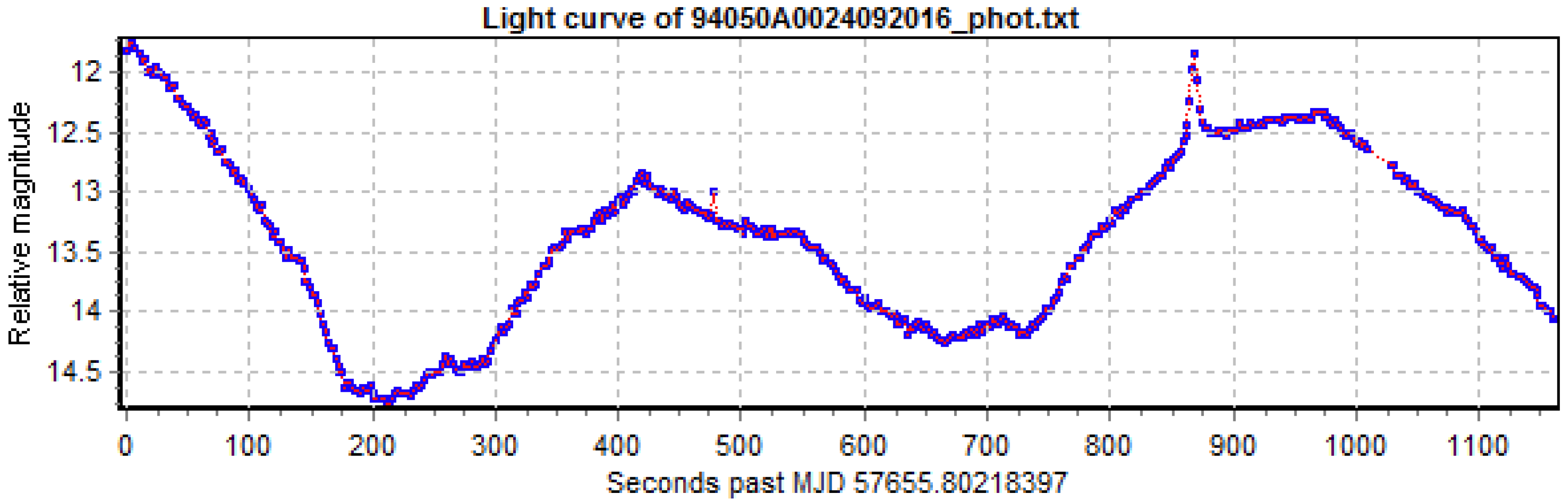
3. Light Curves of GLONASS Satellites

Light curves in the AIUB database are acquired with the Zimmerwald Laser and Astrometry Telescope (ZIMLAT) at the Swiss Optical Ground Station and Geodynamics Observatory in Zimmerwald. The telescope is a 1 m aperture Ritchey-Chrètien telescope on an Alt-Azimuth mount equipped with a back-illuminated CCD camera. The system performs the acquisitions on subframes of 200 × 200 pixels (2.60′ × 2.60′) to increase the light curve sampling and actively track the object in the subframe throughout the observation. The object intensity in the subframes is extracted by an automatic real-time procedure to generate the light curve. No absolute image calibration according to photometric standards is performed on the subframes. The light curve provides relative instrumental magnitudes according to a predefined calibration of the instrument based on measured optical transmissivity and quantum efficiency. If the light curve shows a repeating pattern, its period can be determined. Relative and not absolute photometric values are acceptable in this study since we are interested in the latter periodicity, for which only relative brightness changes are relevant. Linder et al. [26] discuss the advantages and disadvantages of several implemented methods to determine the periodicity in light curves. Figure 1 shows an example of an acquired light curve. A complete processing of the light curve, which includes detrending by applying a second-order polynomial fit and the Phase-diagram Reconstruction Method (PRM) [26], gives the final phase diagram as shown in Figure 2. The PRM is basically an iterative process to find the period with the smallest dispersion in the folded phase diagram. For more details about the overall processing, see [2]. Note that some outliers are present in the light curves, e.g., in Figure 1 at 225 s, and also visible in Figure 2 at 0.05, or, e.g., in Figure 3. Outliers are due to, e.g., bright stars in the background, which, if necessary, can be removed by an automatic screening procedure.

As of November 2020, the database contained light curves of 70 different GLONASS satellites. The light curves have a median duration of around 9.5 min per observation and an exposure time of 1 s. Of the 70 satellites, 51 are first-generation GLONASS (block IIv), while the rest are GLONASS-M satellites. On average, the satellites were observed more than 10 years after decommissioning. From about 83% of the light curves, a period could be extracted, while the remaining are stable (Figure 3) or slow-changing light curves (Figure 4). However, the assignment to the latter categories depends on the length of the available light curves. In the best case, as, e.g., for the satellite in Figure 3, the light curve remains stable during the 20 min maximum configured acquisition time.

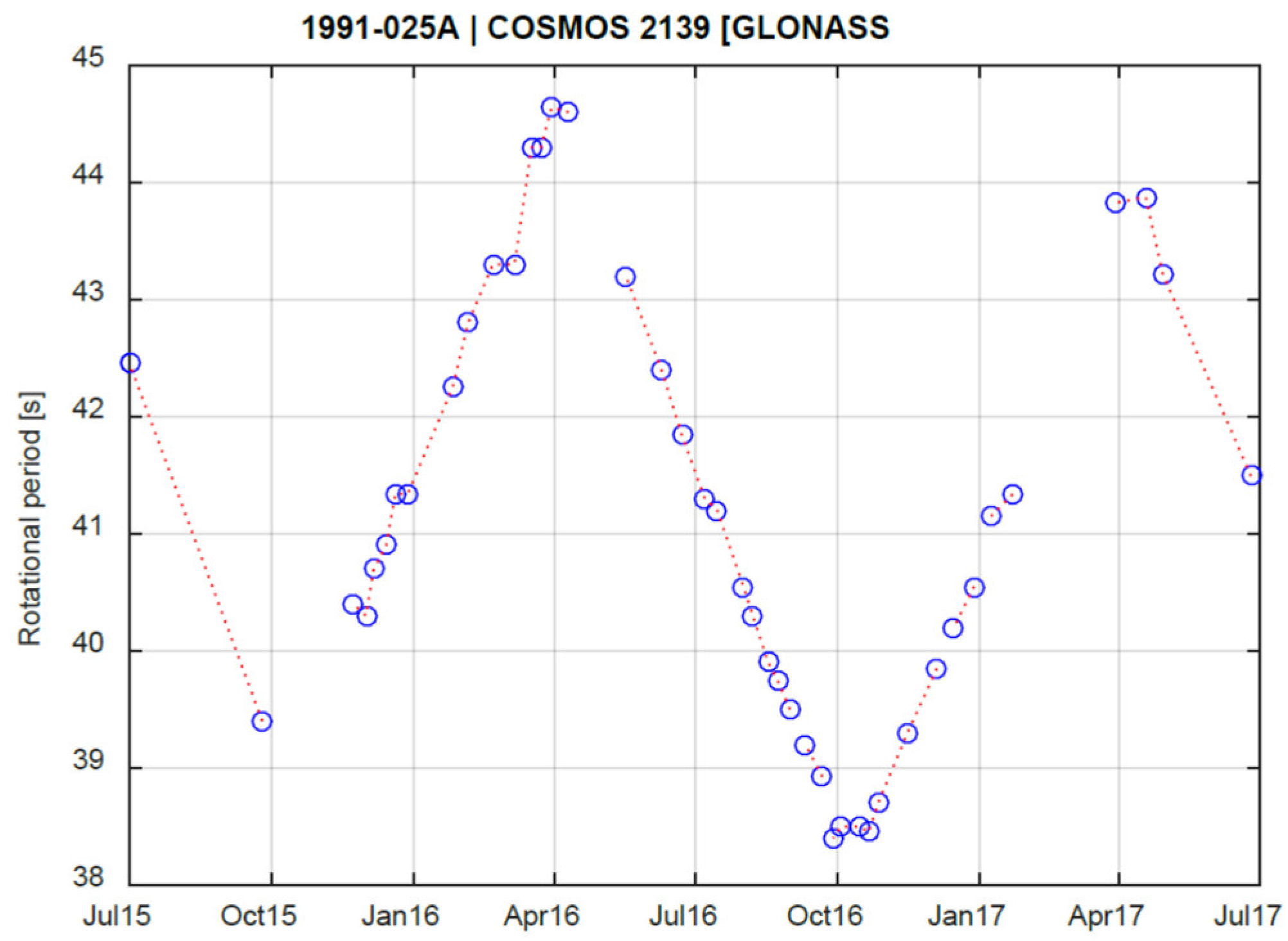
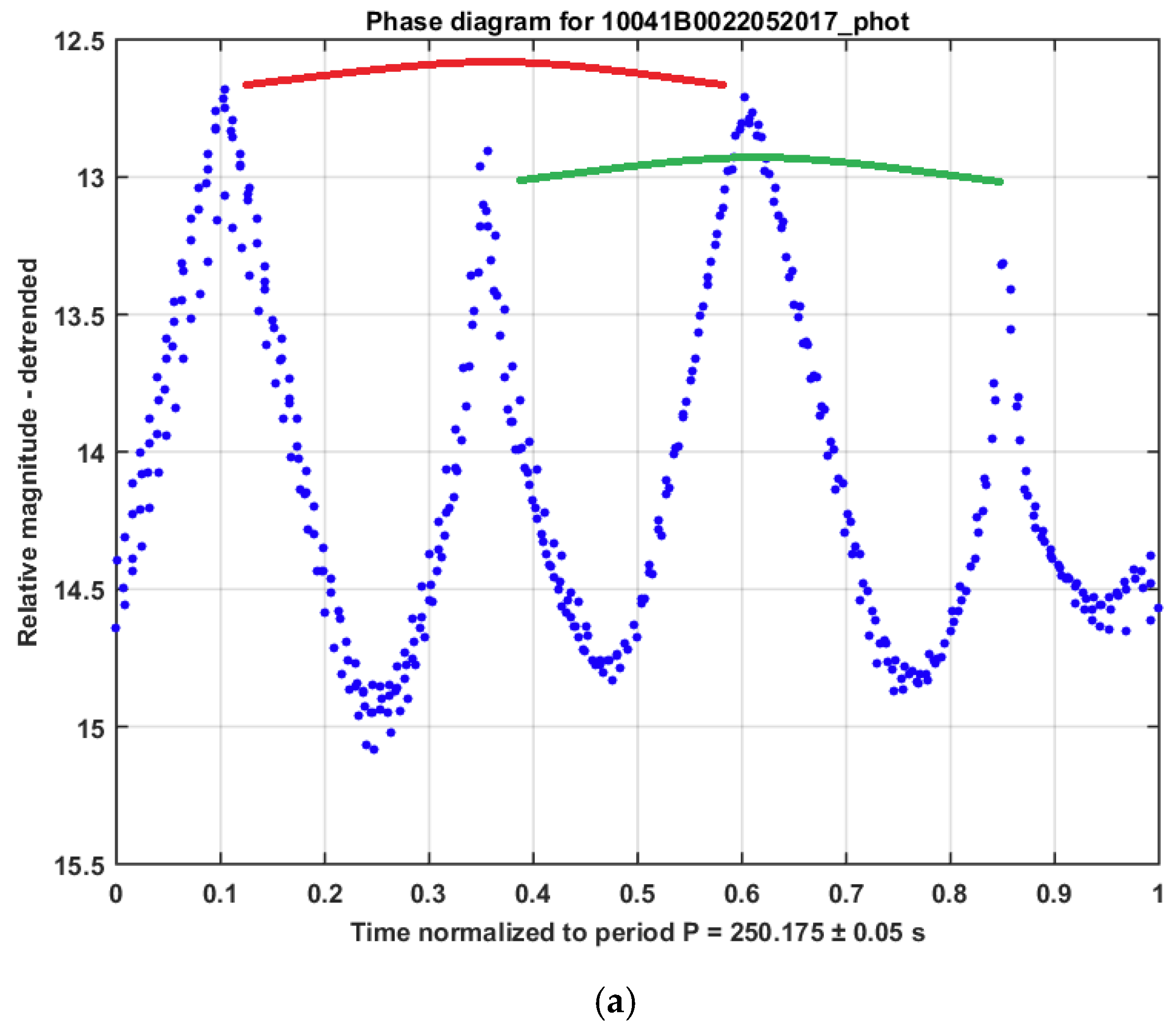
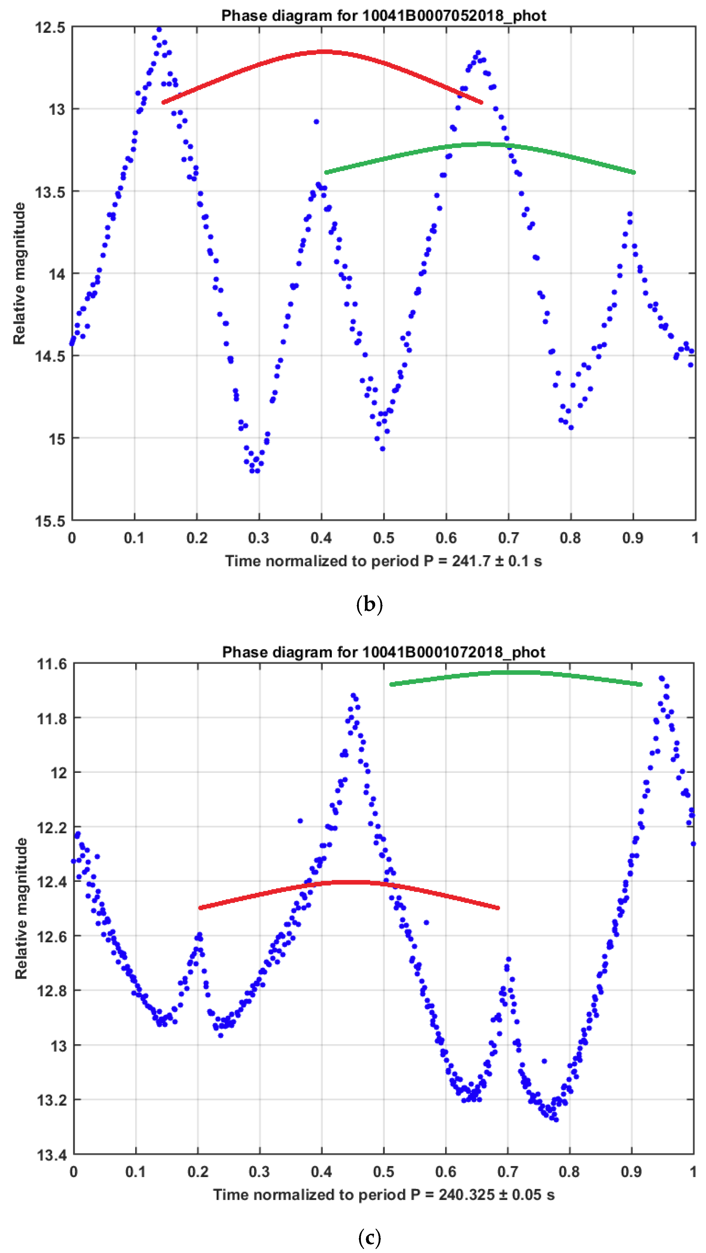
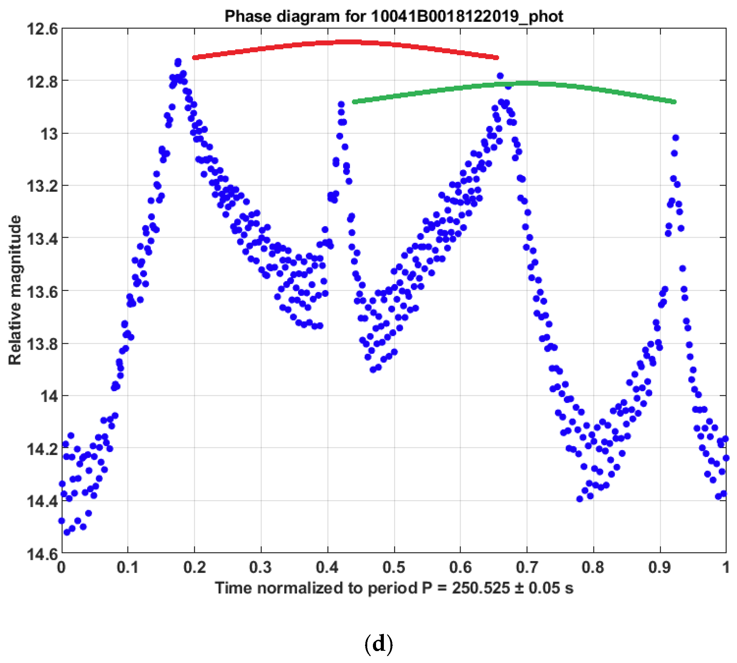
3.1. Cyclic Spin Period

Among those satellites with a clear measured rotation, only 18 show a periodic triangular pattern in the spin period evolution. Other satellites are likely to show the same behavior, but not enough data points were measured, or they indicated a less clear pattern, not necessarily triangular, and with a smaller amplitude. Figure 5 illustrates a typical triangular oscillating pattern in the spin period. Rachman et al. [11] found that the positive/negative slope in the triangular pattern is always roughly similar. Cyclic patterns in spin period evolutions of inactive satellites have been reported, for example, in [14,17]. However, only a few of them show a consistent series of peaks with a triangular shape similar to our case.

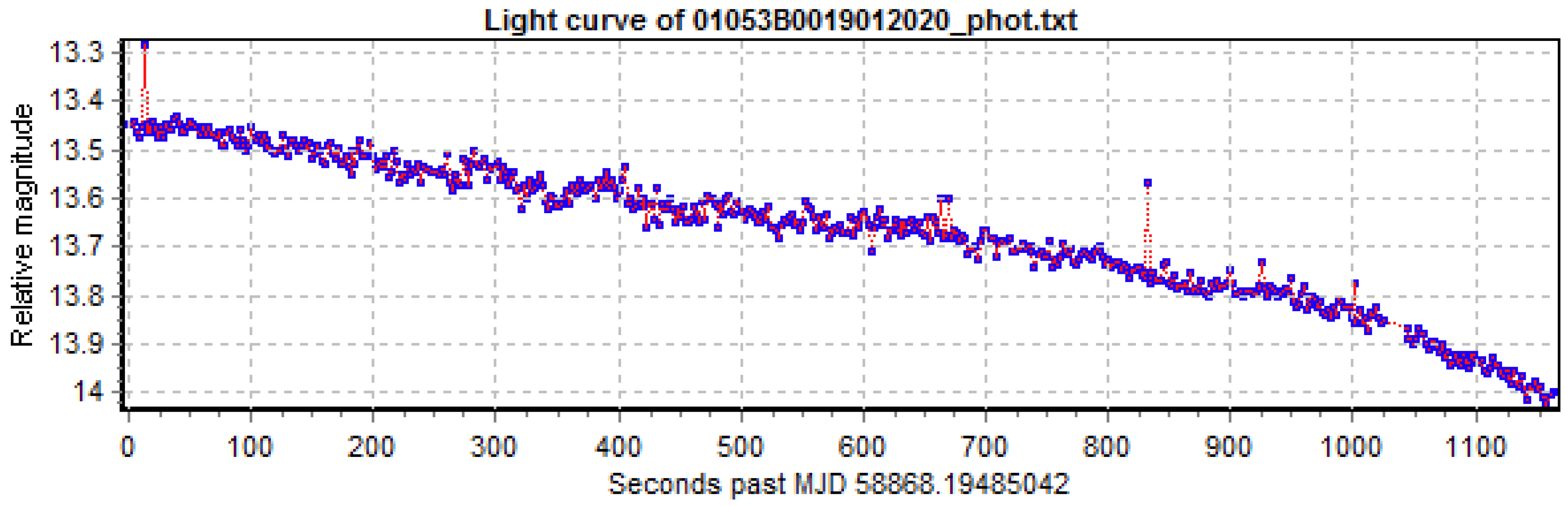
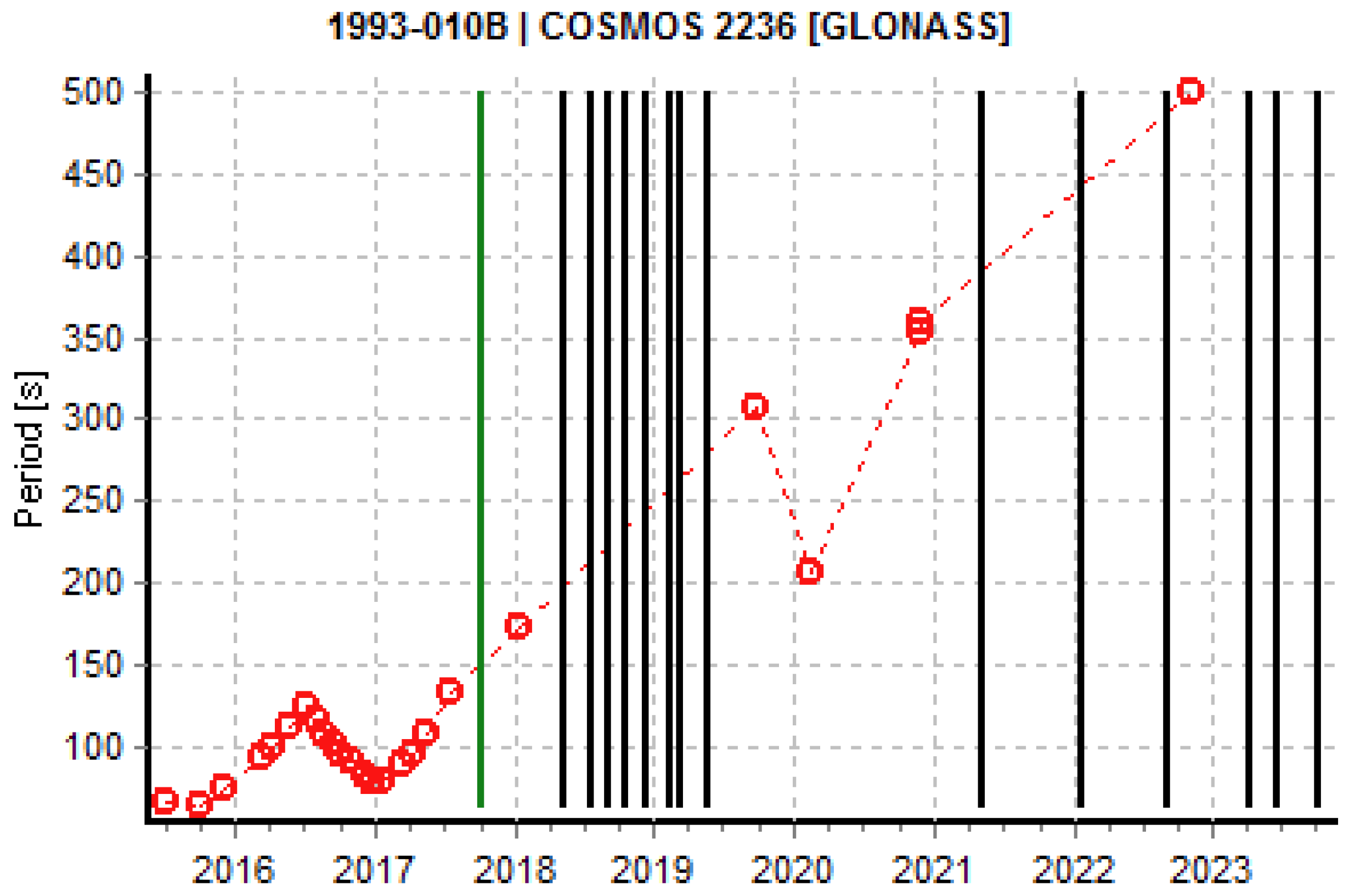
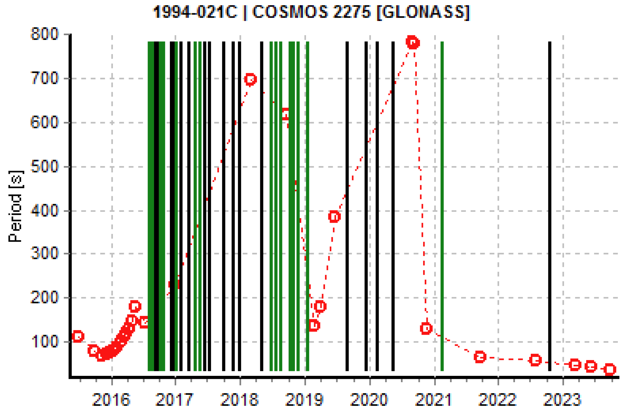
3.2. Cases Without Cyclic Pattern

Stable or slow-changing light curves are interesting because they may show transitions from or to a rotation phase. Some satellites show slow-rotating or stable light curves already in the phase after decommissioning, while others start to show stable light curves after a regular rotation phase. The change from a regular rotation to a slow rotating phase could be a hint for a cycle between a phase of uniform motion (normal rotation) and one with a complex tumbling motion, as in the case of some GEO satellites [22]. The GLONASS satellites COSMOS 2236 (Figure 6) and COSMOS 2275 (Figure 7) start their spin period evolution “normally”, but later their spin periods become much larger and the evolution becomes more complex. This is similar to the case of COSMOS 2411 (Figure 8), although less data are available. Particularly in the first case, the cyclic pattern shows an asymptotic increase towards the peak. This behavior is similar to the one in [22], where the authors propose a mechanism driven by YORP forces and energy dissipation, where the rotation axis is cyclically aligned to the axis of minimum or maximum inertia.

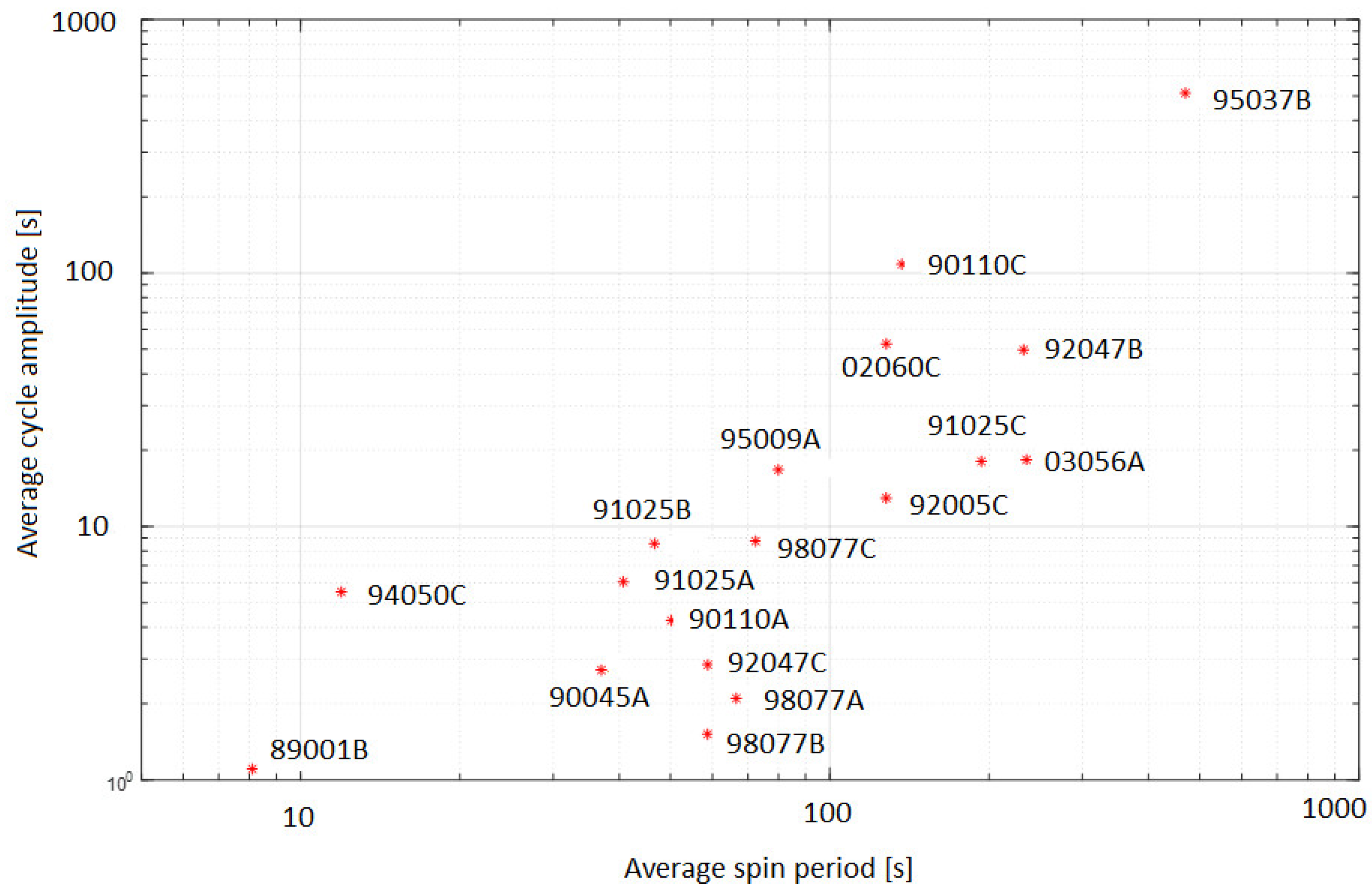
3.3. Light Curve Characteristic

Typically, four peaks (bright reflections) are present in a phase diagram of GLONASS satellites, where the two pairs of peaks have a similar shape but different sizes, as can be seen in Figure 9. On many occasions, one pair is significantly smaller than the other. Within one pair, the distance between the peaks is usually around 180° phase. The sharp profile of the light curves suggests that the peaks are the result of specular reflection, possibly from solar panels. However, the two peaks within one pair have similar brightness and shape. We expect a different reflection from the two sides of a solar panel; one exposing the solar cells and the other probably opaque [27]. Moreover, the presence of four peaks in the GLONASS light curves cannot be explained by the simple two-fold symmetry of the solar panels in parallel configuration.

Those two rationales lead us to presume that this light curve characteristic is caused by the four thermal control flaps related to the radiators, similarly to the hypothesis in [27]. Both type IIv and type M include radiators for thermal control. In [25], the flaps are described as four curved rectangular surfaces equally distributed around the symmetrical axis of the cylindrical bus. The long side of the rectangle is parallel to the bus and is almost as long as the bus, while the width is much smaller. The flaps are fixed on one long side of the rectangle and can be rotated around this axis, i.e., opened for thermal regulation. In terms of opening direction, the flaps are arranged into two pairs (“clockwise pair” and “counterclockwise pair”), where each member of a pair is separated by 180° phase. Figure 10 explains how the arrangement of the radiators on the bus allows an observer to have similar peak profiles within one pair. As we see in the figure, at time = t, the observer sees the satellite in a specific configuration with respect to the radiators (configuration 1), which gives a specific brightness. Half a period later, time = t + 0.5 × P, the observer sees the satellite in the same configuration again with respect to the radiators, hence with similar brightness. This repeating similar configuration corresponds to one of the two pairs in the light curve. The other pair is obtained at time = t + 0.25 × P and time = t + 0.75 × P when the observer sees the satellite in another configuration (configuration 2).

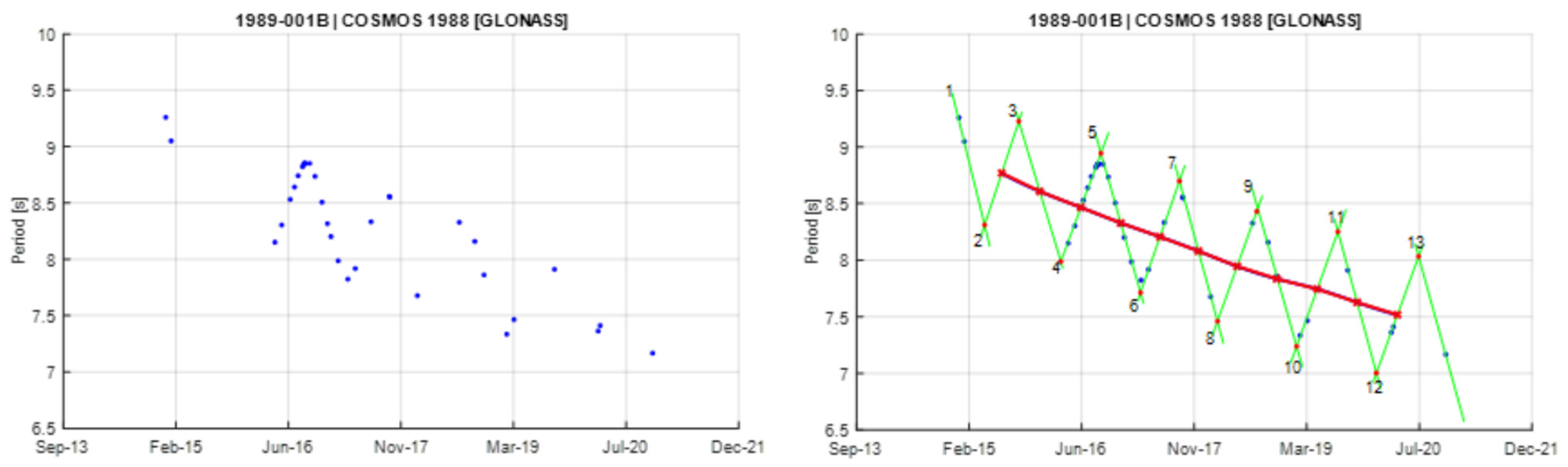
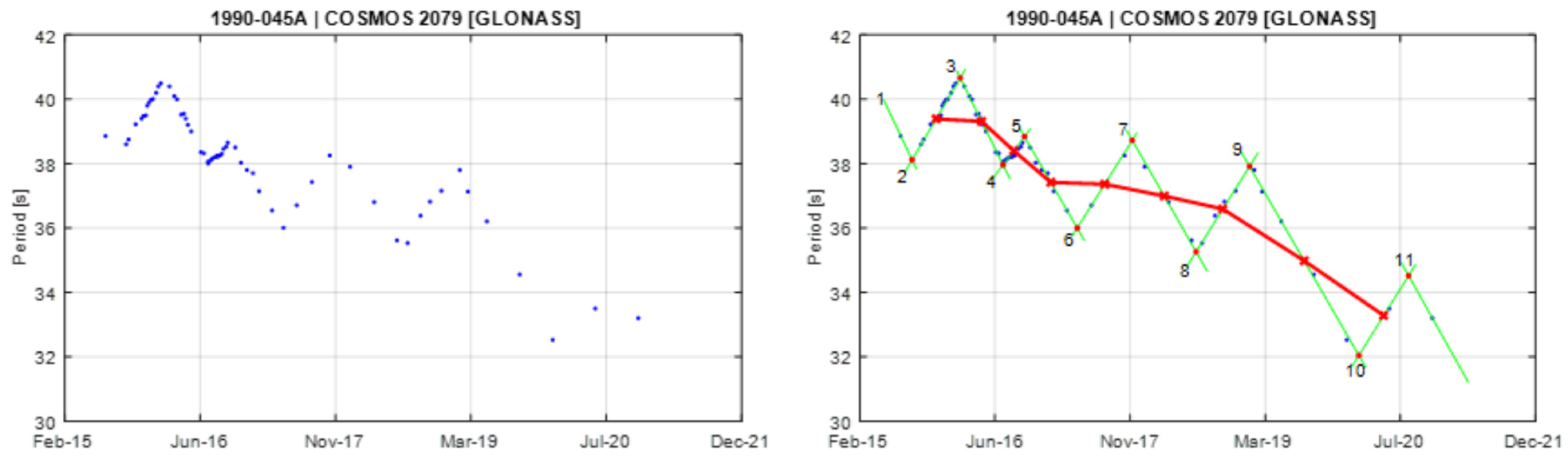
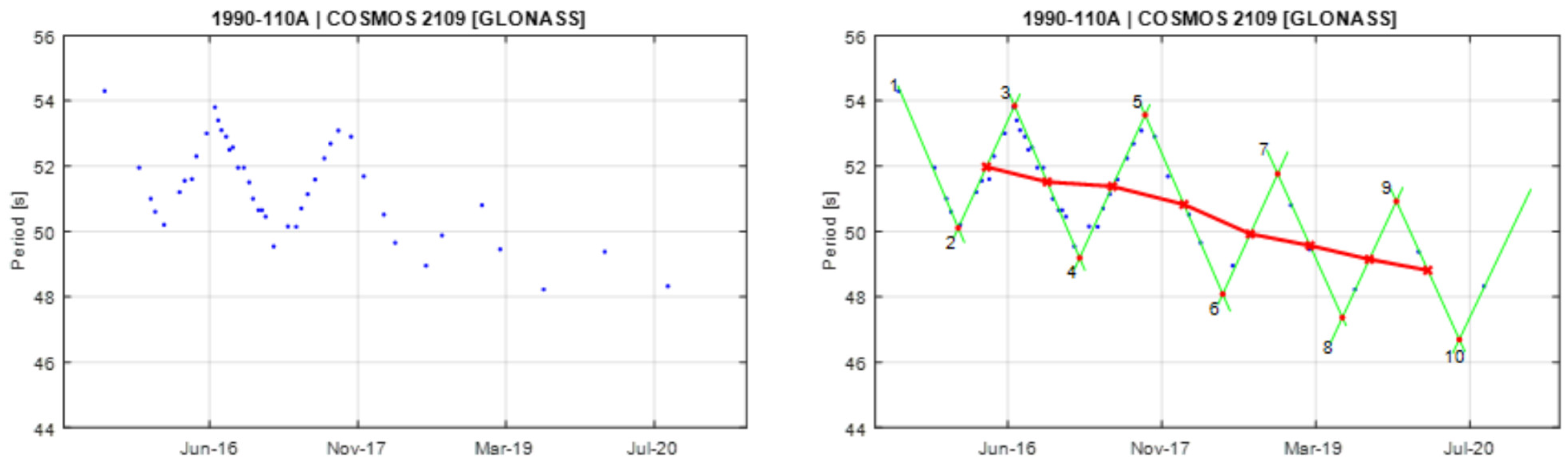
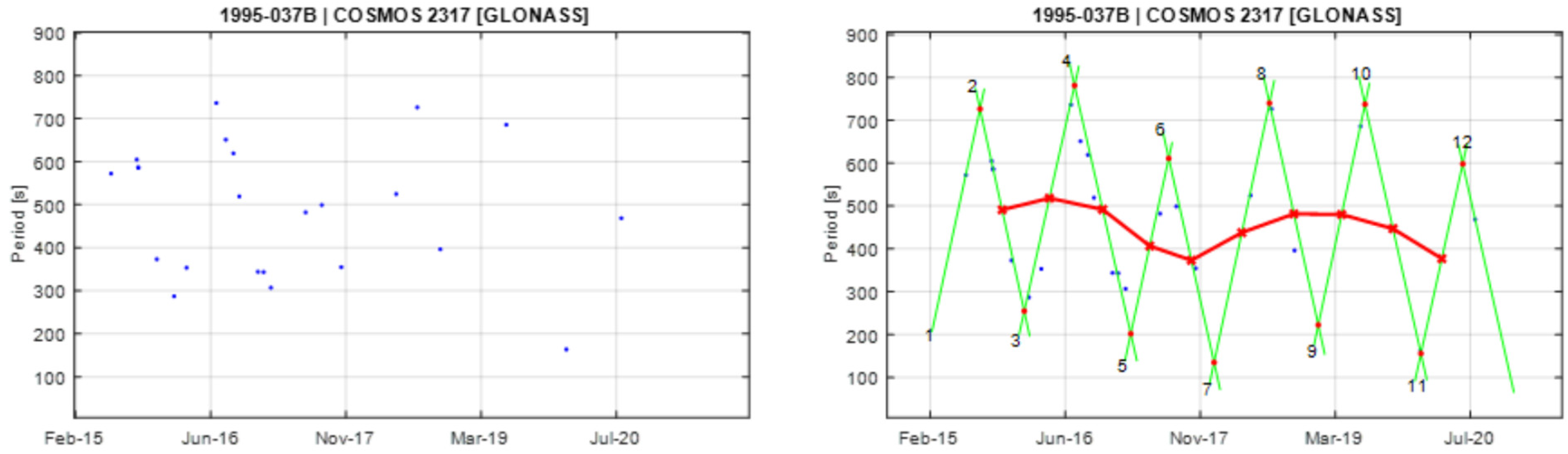
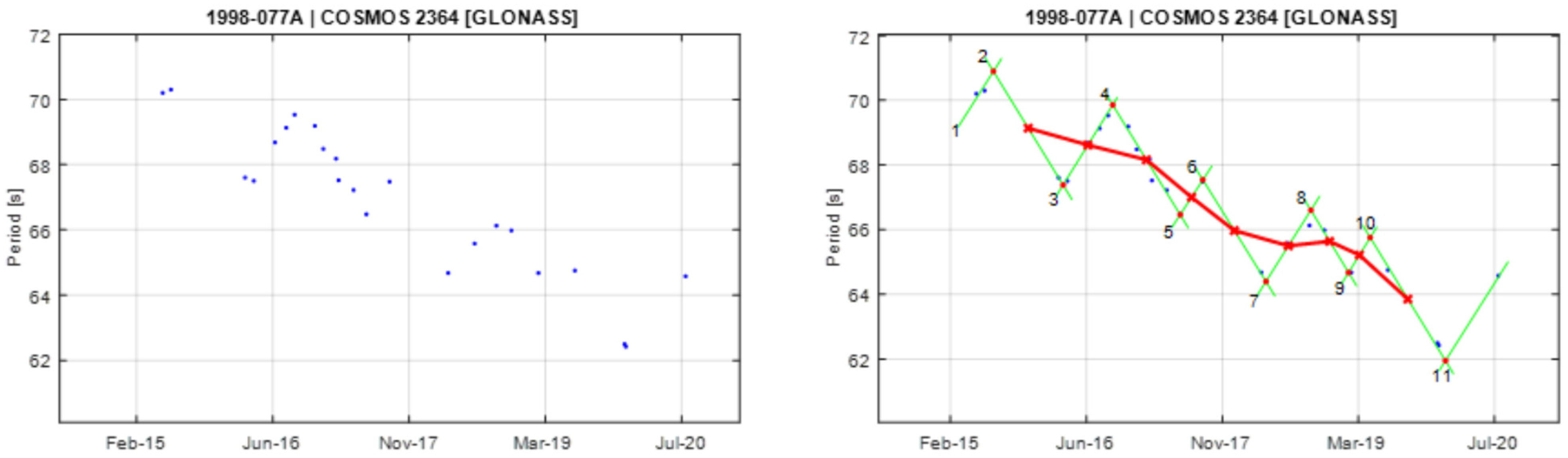
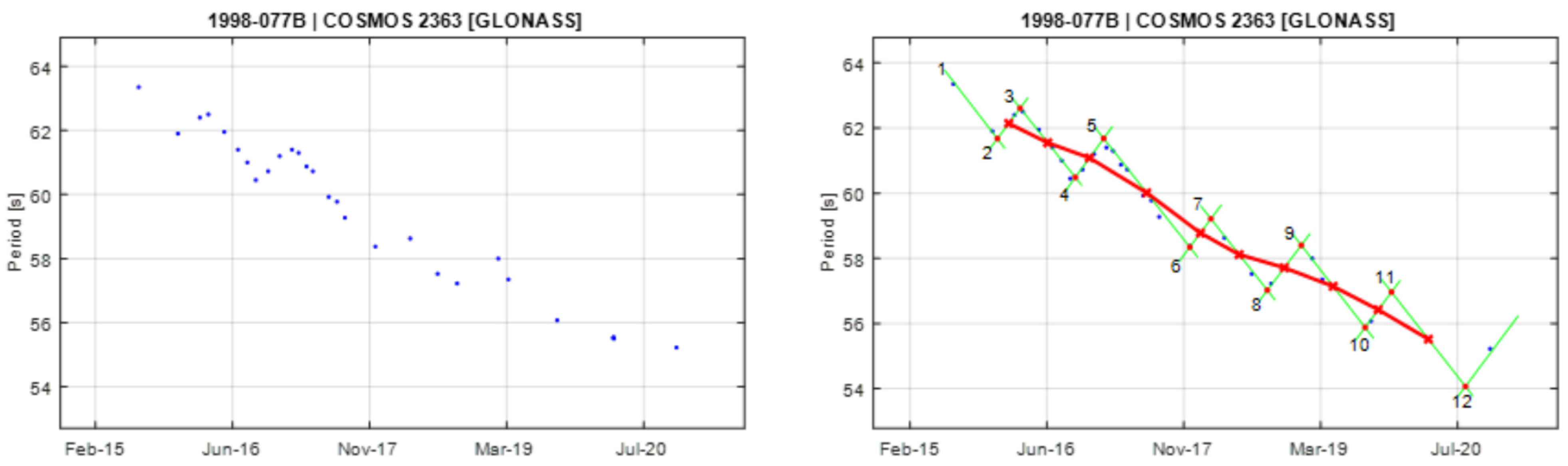
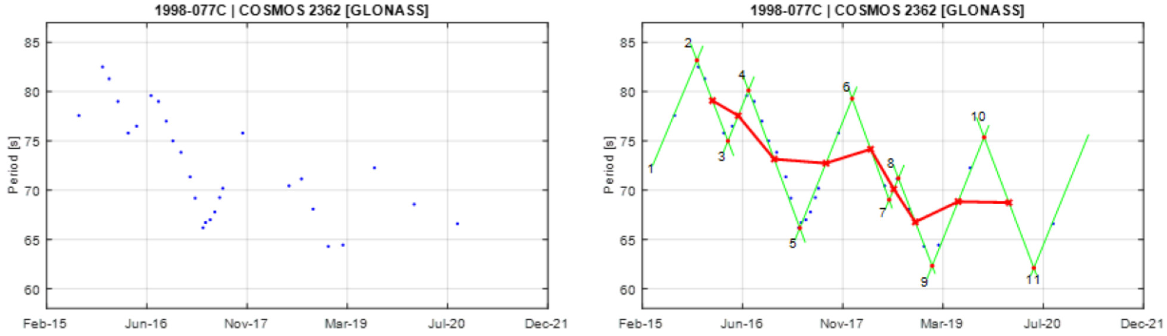
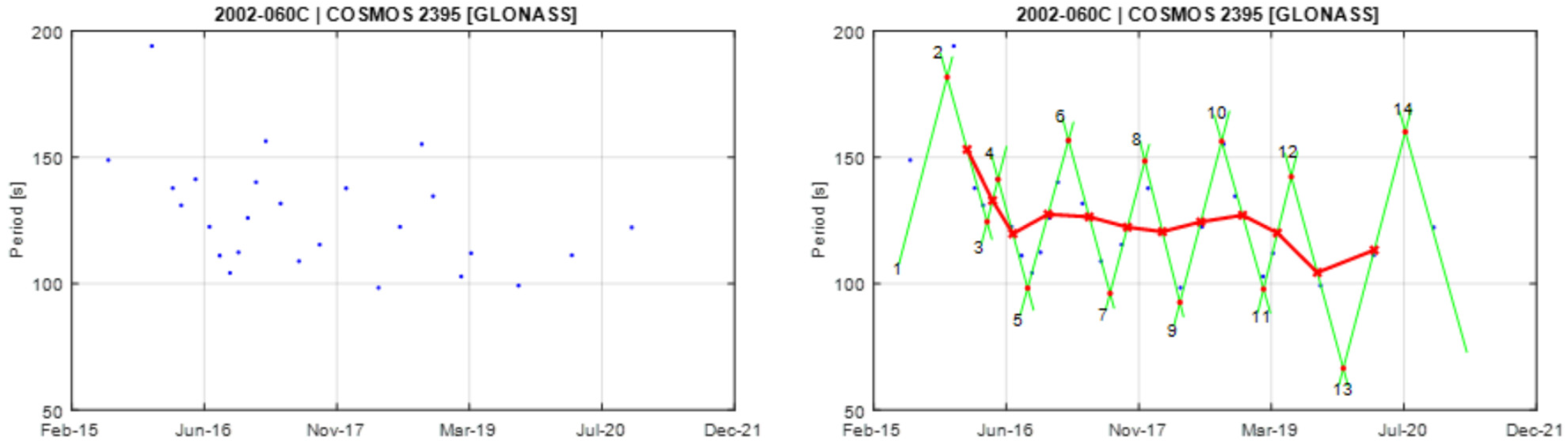
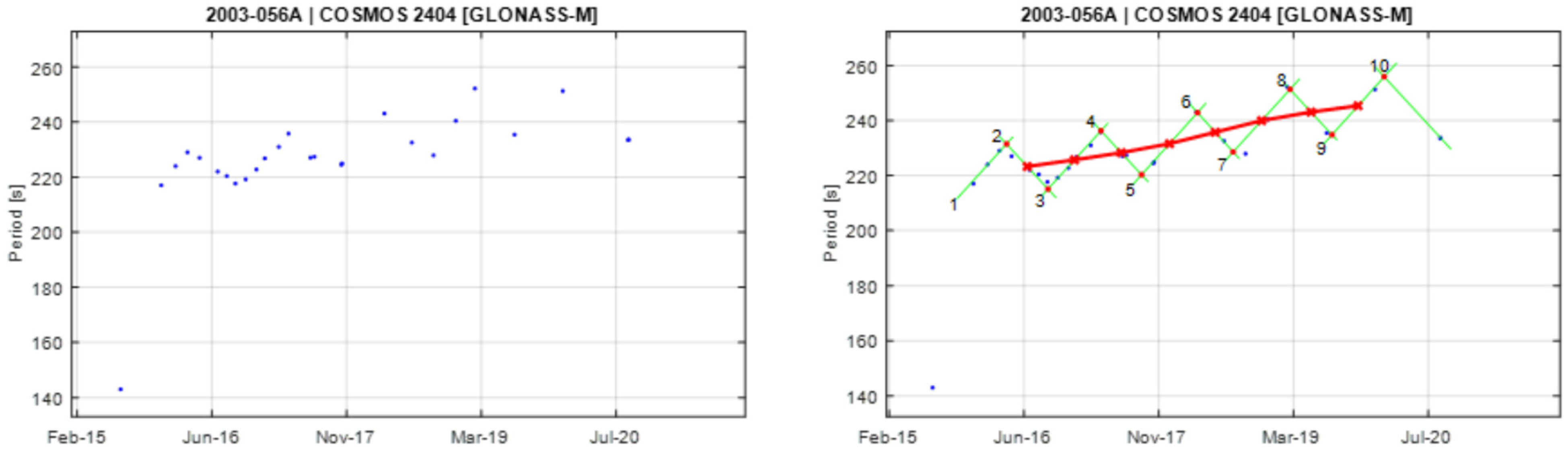
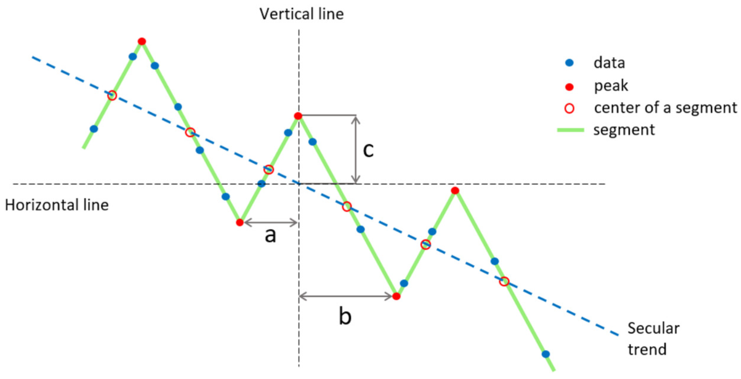
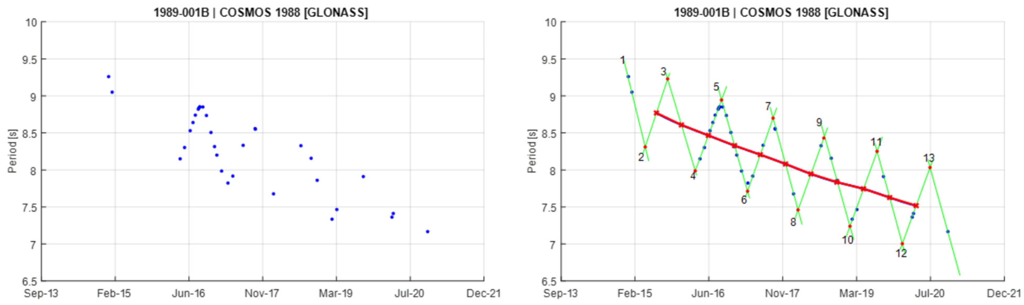
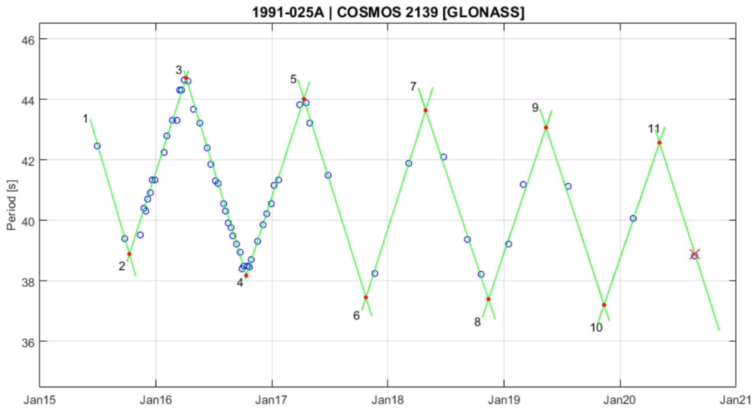
4. Spin Period Evolution

We focus on the 18 inactive GLONASS satellites which show a triangular pattern in their spin period evolution.

Table 1. GLONASS satellites selected for the analysis of the spin period evolution.

No	Satellite	Cospar ID	Type	Launch Date	Decommissioning Date	First Observation Date	Debris Age [yr]
1	COSMOS 1988	1989-001B	IIv	1989-01-10	1992-02-16	2014-12-22	22.85
2	COSMOS 2079	1990-045A	IIv	1990-05-19	1994-04-23	2015-07-06	21.20
3	COSMOS 2109	1990-110A	IIv	1990-12-08	1994-03-17	2015-07-01	21.29
4	COSMOS 2111	1990-110C	IIv	1990-12-08	1996-06-09	2015-07-11	19.09
5	COSMOS 2139	1991-025A	IIv	1991-04-04	1994-09-29	2015-07-01	20.75
6	COSMOS 2140	1991-025B	IIv	1991-04-04	1992-01-06	2015-07-03	23.49
7	COSMOS 2141	1991-025C	IIv	1991-04-04	1992-02-26	2015-07-03	23.35
8	COSMOS 2179	1992-005C	IIv	1992-01-29	1996-10-25	2015-07-06	18.69
9	COSMOS 2204	1992-047B	IIv	1992-07-30	1997-06-27	2015-07-14	18.05
10	COSMOS 2205	1992-047C	IIv	1992-07-30	1994-06-29	2015-07-06	21.02
11	COSMOS 2288	1994-050C	IIv	1994-08-11	1999-08-24	2015-06-28	15.84
12	COSMOS 2307	1995-009A	IIv	1995-03-07	1999-09-10	2015-06-19	15.77
13	COSMOS 2317	1995-037B	IIv	1995-07-24	2001-01-24	2015-06-17	14.39
14	COSMOS 2364	1998-077A	IIv	1998-12-30	2002-07-08	2015-05-12	12.84
15	COSMOS 2363	1998-077B	IIv	1998-12-30	2003-12-19	2015-07-13	11.56
16	COSMOS 2362	1998-077C	IIv	1998-12-30	2003-10-20	2015-07-16	11.74
17	COSMOS 2395	2002-060C	M	2002-12-25	2008-01-12	2015-06-23	7.44
18	COSMOS 2404	2003-056A	M	2003-12-10	2009-06-18	2015-07-16	6.08

displays basic data of the selected satellites. The debris age is defined as the difference between the decommissioning date and the date of the first observation. Most of the objects are of type IIv; only two of them are of type M. All the objects have more than 20 observed spin periods and have been observed for five or six years.

In characterizing the oscillating pattern of the spin period evolution, we use the assumption that the variations in the evolution can be empirically modeled by a series of triangular shapes having similar slopes for the left and right segments of the triangle. The segments are computed by linearly fitting observed period values. Figure 11 illustrates the basic model for the simplest case where all the triangular shapes are similar, and the secular evolution trend is linear. For each of the triangular shapes, we identify the peaks (or local extremes) of the oscillation. These are located at the intersection between two adjacent segments. We calculate the average spin period from the values of all peaks. We define the amplitude of a cycle as A = 2c, where c is the vertical distance between a peak and the line joining the center of two adjacent segments, and we calculate the average cycle amplitude. The periodicity of a cycle P is the time difference between two adjacent top peaks or two adjacent bottom peaks, i.e., P = a + b, and we compute the average cycle period. We also calculate the average secular trend of angular velocity ω per year and the average segment change of angular velocity per month within the segment. To create the whole series of triangular shapes, we first begin with a principal triangular shape, created using the two adjacent segments that possess the largest number of data points. This principal shape serves as a base for creating the rest of the series.

Figure 12 shows a comparison between the observational data of one of the objects and its empirical model. For this case, we select Segment 4 and Segment 5 to create the principal triangular shape. As can be seen on the left side of the figure, the first two segments are the only segments with sufficient data points to create the base. Despite this shortage, the right side of the figure shows how the resulting model nicely fits the whole dataset. The figure also shows that the average secular trend is more or less linear.

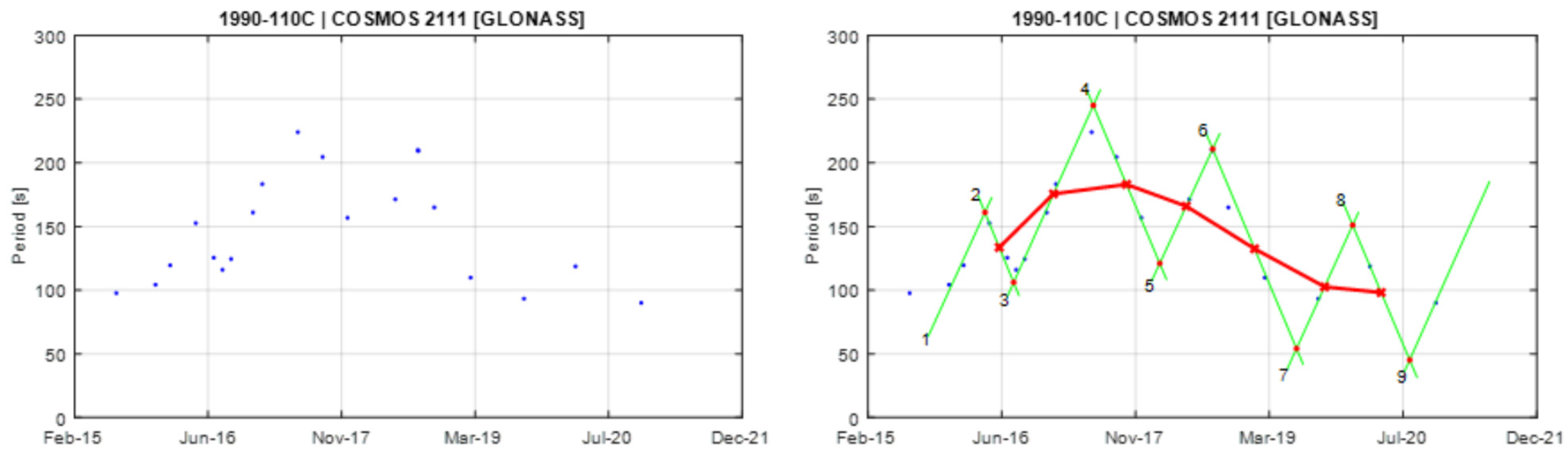
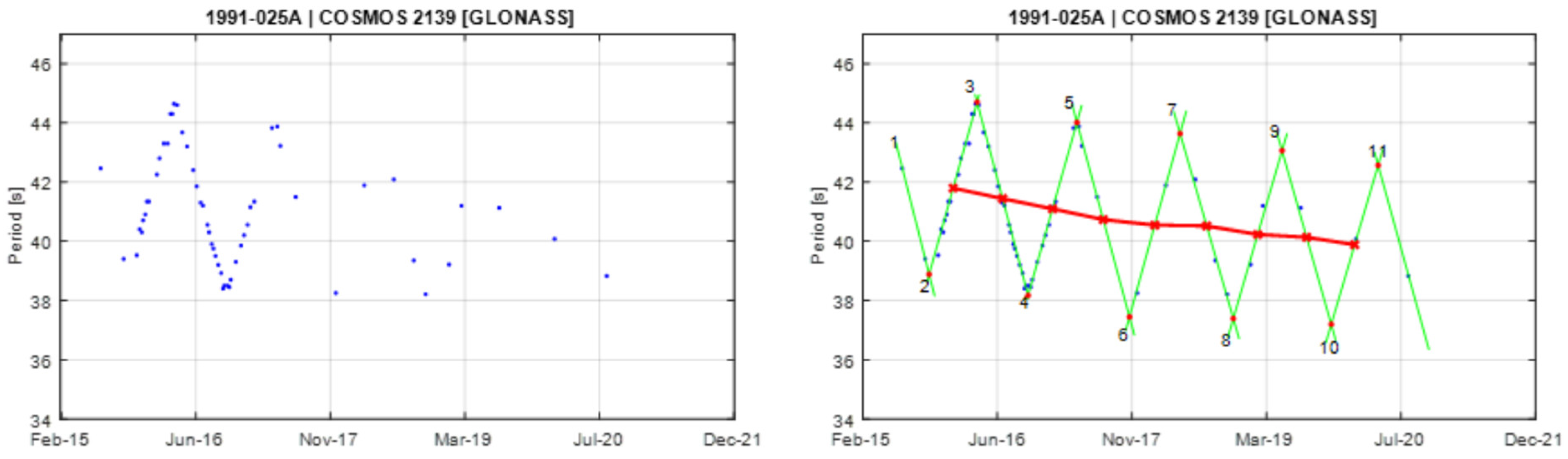
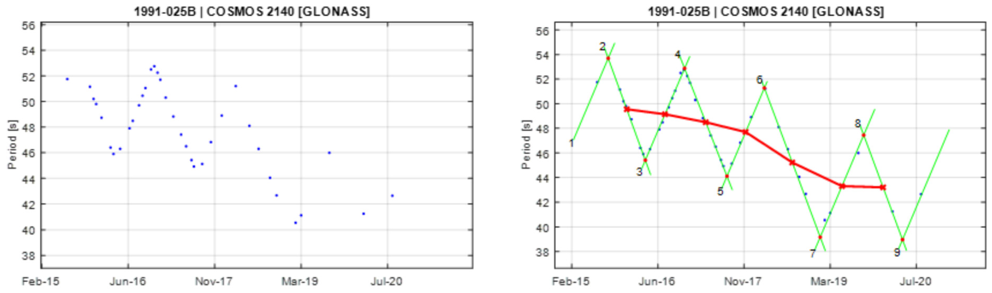
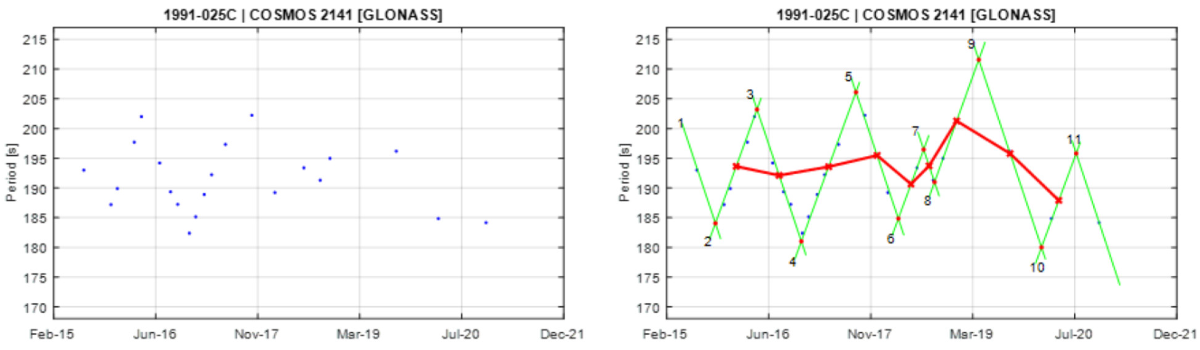
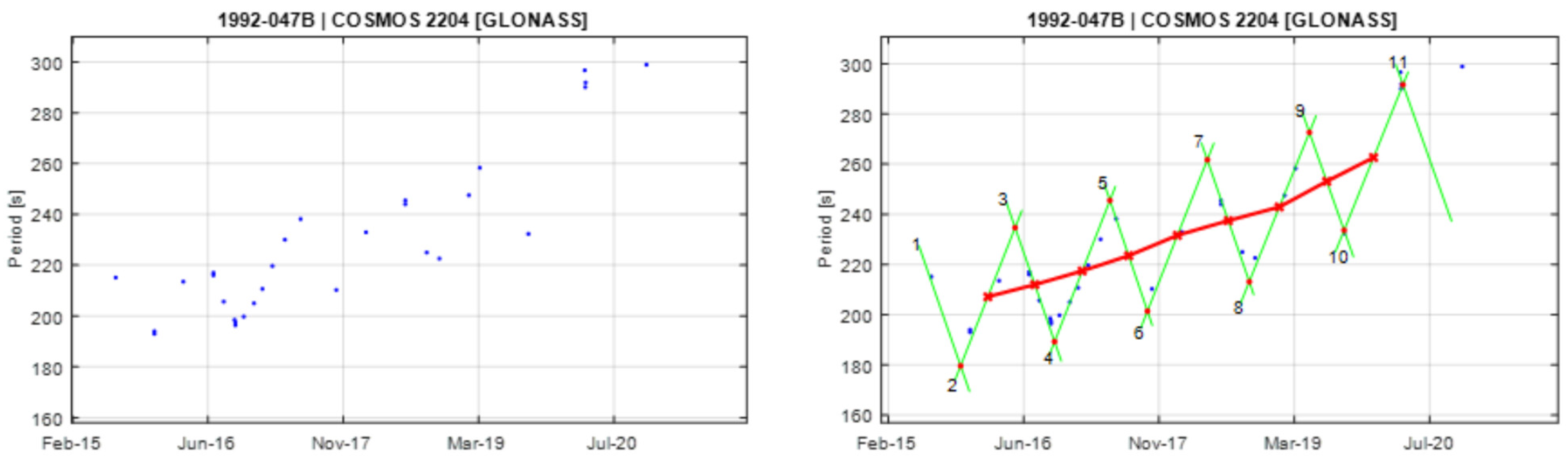
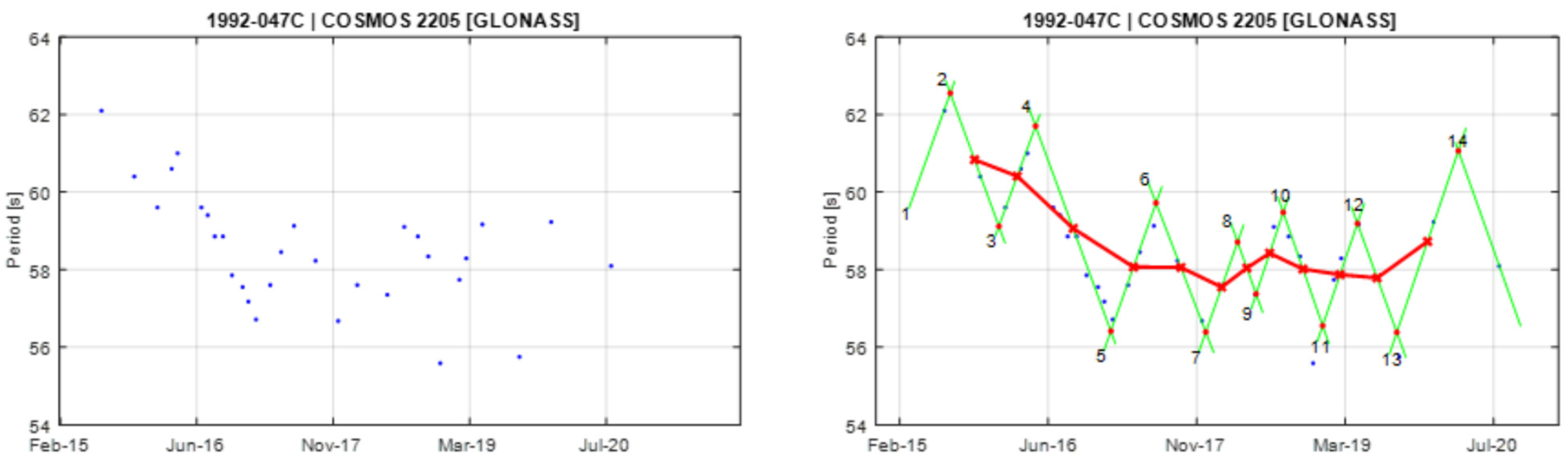
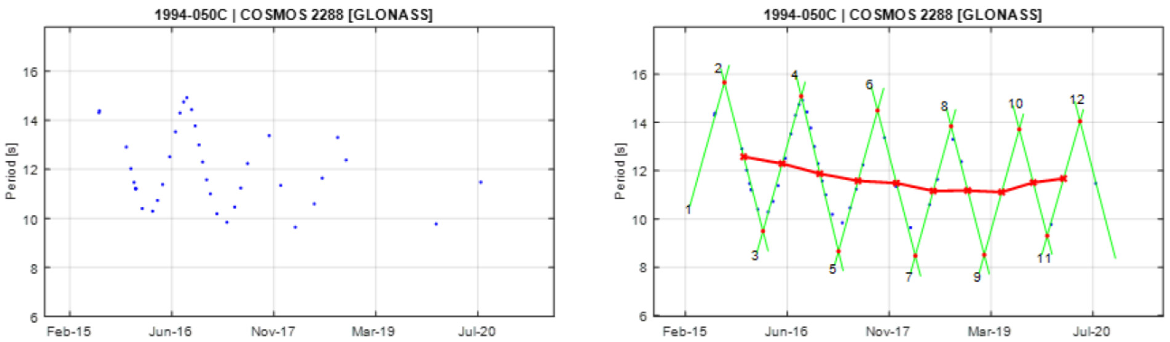
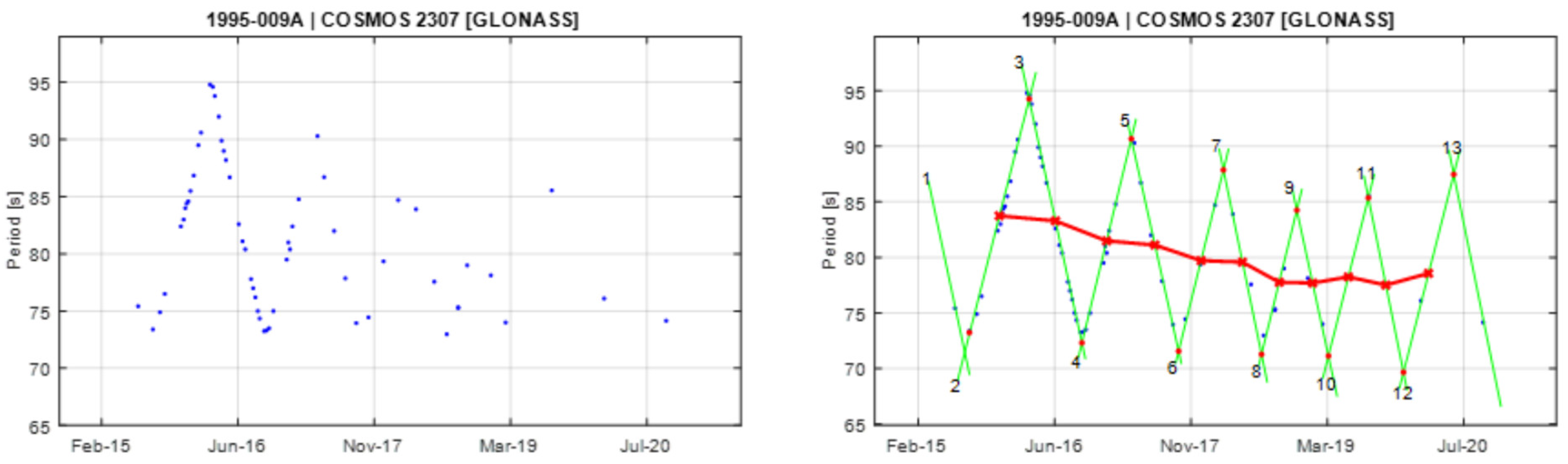
4.1. Spin Period Prediction

Given the regularity of the pattern for some satellites, we can use the empirical model to extrapolate the spin period at an epoch outside the interval of the observations. As an example, let us estimate the spin period of the last observation of COSMOS 2139 on 24 August 2020 and compare the result with the one from the database. We take the dates and coordinates of all the peaks as inputs, and we derive the average slope of the connected segments and of the secular change. Using the derived slope, we extrapolate the spin period for the date of 24 August 2020, and we find 38.867 s. This value is reasonably close to the one from the database, which is 38.825 s. Figure 13 shows the observational data and its model used in this example. For COSMOS 2139, as well as for a few other satellites, like COSMOS 1988, COSMOS 2109, COSMOS 2204, COSMOS 2363, and COSMOS 2404, the prediction is possible because they show a nearly linear trend (see Appendix A). In this case, the error in fitting the measurements in the base triangle affects the predicted value. Other objects deviate from a linear trend and show significantly shorter or longer segments that cannot be explained by a simple model and do not allow a spin period prediction.

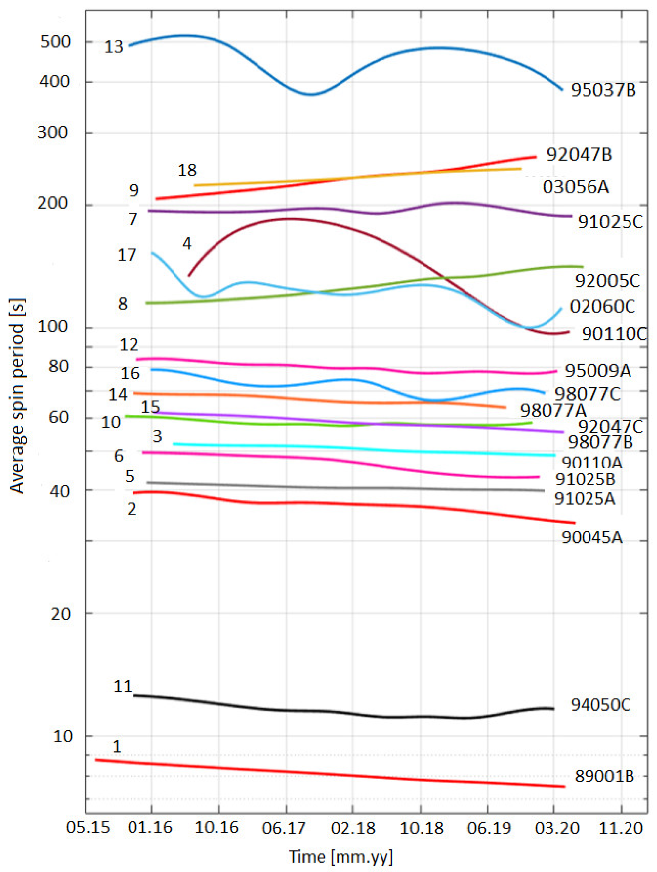
4.2. Statistics of Spin Period Evolution

Table 2. Average characteristics of the spin period evolution. ω is the angular velocity.

No	Cospar ID	Average Spin Period [s]	Average Velocity [°/s]	Average Cycle Amplitude [s]	Average Cycle Period [yr]	Secular Trend Change of ω Per Year [°/(s·yr)]	Average Segment Change in ω Per Month [°/(s·mo)]
1	1989-001B	8.11	44.68	1.10	0.95	1.408	1.040
2	1990-045A	37.00	9.77	2.71	1.13	0.340	0.111
3	1990-110A	50.17	7.19	4.26	1.11	0.120	0.089
4	1990-110C	136.81	3.59	108.43	1.25	0.359	0.394
5	1991-025A	40.71	8.89	6.05	1.02	0.095	0.212
6	1991-025B	46.62	7.83	8.56	1.35	0.300	0.179
7	1991-025C	193.41	1.86	18.06	1.09	0.001	0.028
8	1992-005C	127.80	2.84	12.95	0.90	−0.143	0.056
9	1992-047B	232.31	1.58	49.73	0.97	−0.093	0.060
10	1992-047C	58.82	6.13	2.84	0.78	0.059	0.068
11	1994-050C	11.94	32.05	5.52	0.96	0.634	2.680
12	1995-009A	79.92	4.56	16.74	0.87	0.083	0.182
13	1995-037B	469.58	1.17	513.24	0.98	0.028	0.243
14	1998-077A	66.55	5.42	2.10	0.95	0.109	0.033
15	1998-077B	58.76	6.14	1.51	0.94	0.165	0.034
16	1998-077C	72.38	5.02	8.76	0.98	0.181	0.109
17	2002-060C	127.90	3.05	52.56	0.79	0.140	0.304
18	2003-056A	235.17	1.53	18.32	0.96	−0.046	0.021

shows the average characteristics of the spin period evolutions of the objects. Observational data and empirical models for all the objects are given in Appendix A. The statistics for the results are indicated in

Table 3. Statistics of the results in Table 2.

Statistics	Average Spin Period [s]	Average Velocity [°/s]	Average Cycle Amplitude [s]	Average Cycle Period [yr]	Absolute Value of Secular Trend Change in ω Per Year [°/(s·yr)]	Average Segment Change in ω Per Month [°/(s·mo)]
Maximum	469.58	44.68	513.24	1.35	1.408	2.680
Minimum	8.11	1.17	1.10	0.78	0.001	0.021
Mean	132.82	8.13	70.88	1.01	0.227	0.395
Median	69.47	5.22	8.66	0.96	0.130	0.110

. The average spin period is between 8.11 s and 469.58 s. This is similar to the average cycle amplitude, with a range from 1.10 s to 513.24 s. The average cycle period remains between 0.78 years (285.10 days) and 1.35 years (494.22 days), and its mean and median values are close to 1 year (365.25 days). The average segment change in ω per month represents the angular acceleration, which ranges from 0.021°/s to 2.680°/s.

Figure 14 shows the long-term variation in the average spin period. We can see that most of the objects have a diminishing trend, i.e., they tend to rotate faster during their lifetime. In particular, all the objects with a spin period less than 100 s show a decrease in the spin period, while the remaining objects seem not to show any specific trend.

The cycle amplitude and the secular trend seem to be correlated with the average spin period, as shown in Figure 15 and Figure 16. The coefficients of correlation are 0.84 and −0.45, respectively. Note that the latter correlation is about 0.93 if angular velocity instead of spin period is considered. Similarly, the segment change correlation with the spin period is 0.75. This means that objects with higher spin rates tend to have a higher change in the spin rate, or angular acceleration, in both the annual cycle and the secular trend.

5. Simulations of the Spin Period Evolution

5.1. Simulation Setup

The idea of the following simulations is to be able to roughly replicate the pattern of spin rate evolution of one of the objects. Since most of the objects are GLONASS satellites of type IIv, we built our model based on that type. We picked, rather arbitrarily, one of the objects as the reference, namely COSMOS 2139, which was launched on 4 April 1991 and retired on 29 September 1994. Apparent spin periods from the database are available from 1 July 2015.

We assume that the object is a rigid body and that there are no effects from attitude control system activation, tank sloshing, and specific impact or leakage events.

Considering the similarity between type IIv GLONASS satellites and GORIZONT satellites, we adopted a simple model of the latter satellite, described in [20]. The model considers a cylinder shape for the bus and two rectangular plates as wings for the solar panels. In

Table 4. Basic physical properties of the satellite model.

Property	Value
Mass	2110 kg
Bus length	5 m
Bus diameter	2 m
Solar panel length (one side)	5.45 m
Solar panel width (one side)	3.73 m
Solar panel depth	5 cm

, the basic properties of the model are indicated. The axis of the solar panels runs exactly through the center of the bus. In the basic configuration, both solar panels are parallel to each other, and they are orthogonal to the long axis of the body. The radiator flaps described in Section 3.3 were not included in the model, since they have a smaller reflecting area compared to the solar panels and the bus.

Simulations of the rotation rate under different conditions were performed using iOTA (in Orbit Tumbling Analysis) [28]. This software performs the propagation of the orbit and attitude motion (six degrees-of-freedom). The inputs for iOTA are surface geometry, mass, center of mass position, moments of inertia, radiation absorption coefficient, and diffuse reflection coefficient of the satellite model. Center of mass and moments of inertia were calculated using the open-source software MeshLab (Version MeshLab-2020.12) (on www.meshlab.net (accessed on 20 December 2020)). Unless indicated otherwise, the default values of 0.7 for absorption and 0.2 for diffuse reflection were assumed.

Modeling the effect of different optical properties of the satellite components at the time of the simulations was not yet supported by iOTA. Therefore, for those simulations, another software called D-SPOSE Version 1.0.1 was employed. The software was developed for the analysis and prediction of the rotational motion of space debris to determine the evolution over a time scale of years [29]. Although both tools support different perturbation forces, in the orbital model, only the gravitational force of the Earth point mass was taken into account, while in the attitude model, only the solar radiation pressure (SRP) was considered, since this is predominant for the attitude behavior of the selected object in that orbit regime [30]. The total torque ${\mathit{N}}_{SRP}$ due to SRP is given by the sum over all illuminated facets of the satellite ${\mathit{N}}_{SRP}=\sum _i{\mathit{R}}_i\times {\mathit{F}}_i$, where a ${\mathit{R}}_i$ is the vector from the satellite’s center of mass to the i facet and ${\mathit{F}}_i$ is the applied force [31]:

$${\mathit{F}}_i=-{\displaystyle \frac{E_0}{c}}\left(\left(1-C_s\right)\mathit{S}+2\left(C_s\cos \theta +{\displaystyle \frac{1}{3}}{C}_d\right){\mathit{N}}_i\right)A_i\cos {\theta }_i$$

(1)

$E_0$ is the solar constant, $c$ is the speed of light, $\mathit{S}$ is the unit vector from the spacecraft to the Sun, ${\mathit{N}}_i$ is the unit outward normal to the i facet with area $A_i$, and ${\theta }_i$ is the angle between $\mathit{S}$ and ${\mathit{N}}_i$. The coefficients $C_s$ (specular reflection), $C_d$ (diffuse reflection), and $C_a$ (absorption) obey the relation $C_s+C_d+C_a=1$.

Three parameters are crucial for the initial conditions of the simulations:

• The orientation of the solar panels with respect to the body frame and their canting angle;
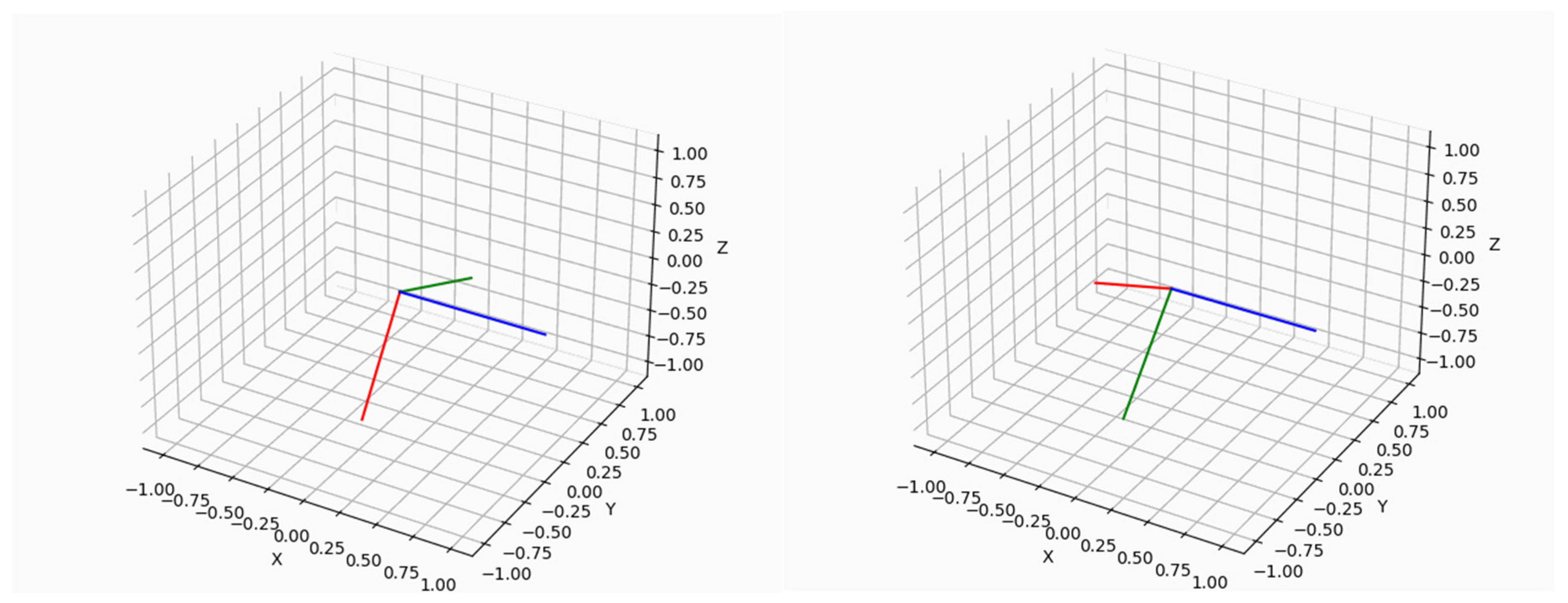
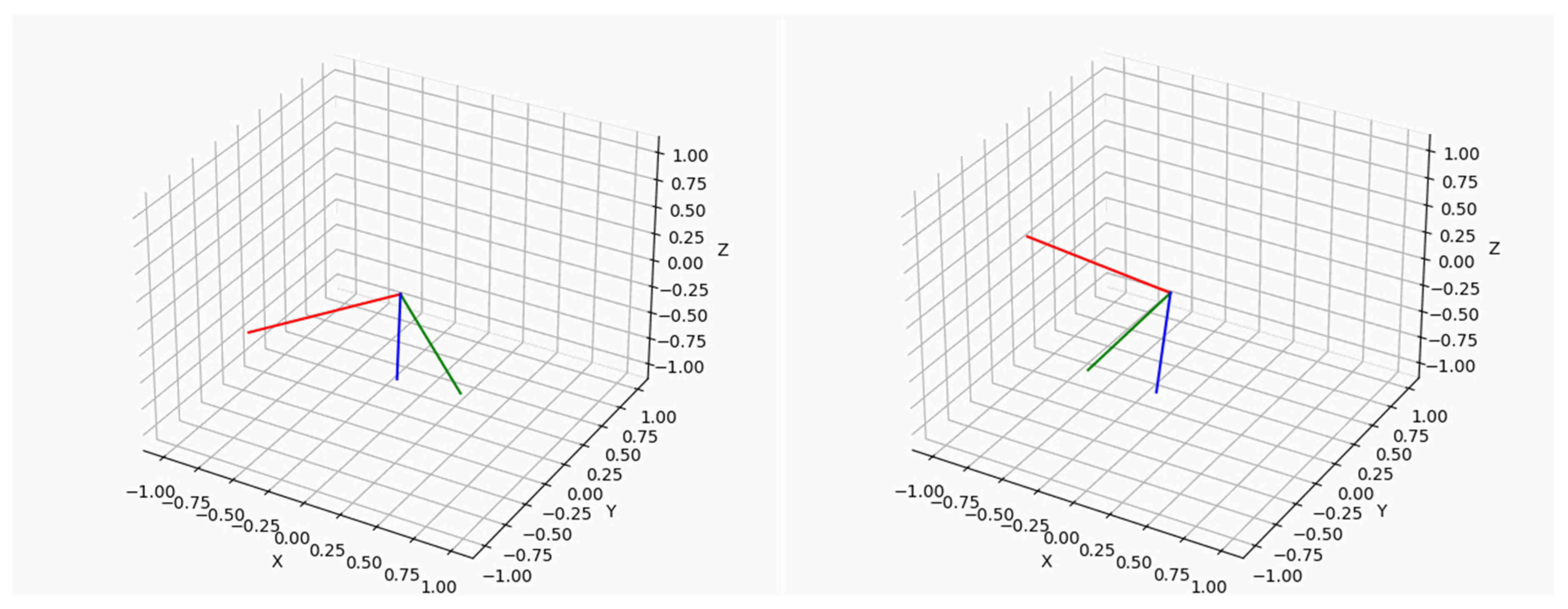
• The initial orientation of the satellite with respect to the orbital frame;
• The initial angular velocity vector of the rotation.

The canting angle (angle between the two solar panels) is important for providing asymmetry to the satellite model. According to [14], with symmetric solar panels of the same size and reflectivity and no canting angle, there would not be any net SRP torque. In [20], a canting angle between 9° and 22° was adopted to obtain the necessary torque. In our simulations, we assume a 10° canting angle. The initial satellite orientation is specified in the next section, while the initial angular velocity varies in the different simulations.

Two-line element orbital data for the simulations was obtained from the Space-Track website (www.space-track.org, accessed on 23 March 2025), and the positions and velocities of the satellite were computed for the starting epoch of the simulations on 1 September 2015 at 21:00:00 UTC. COSMOS 2139 is moving in a circular medium Earth orbit with a radius of around 19,180 km from Earth’s center and an inclination of 65.48°.

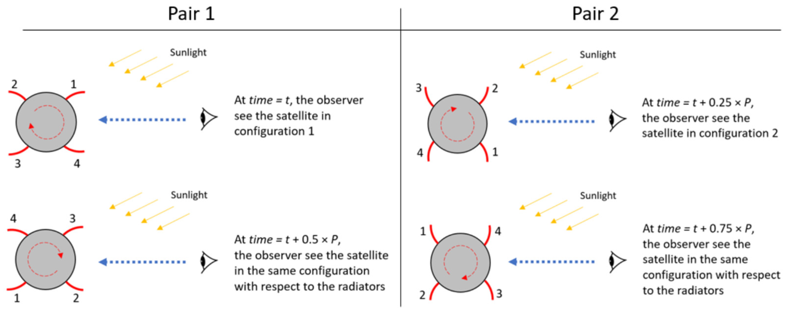
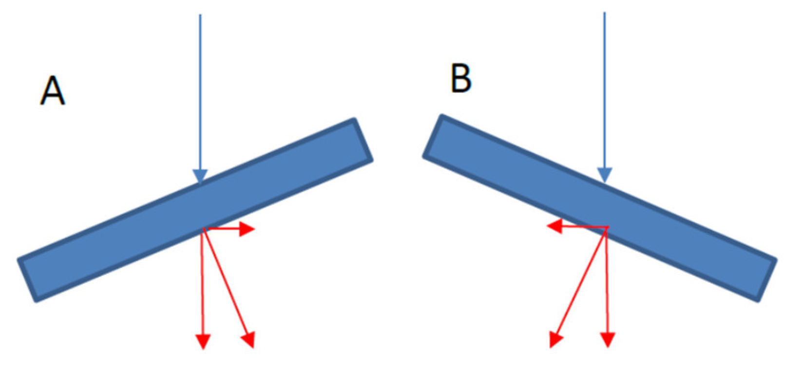
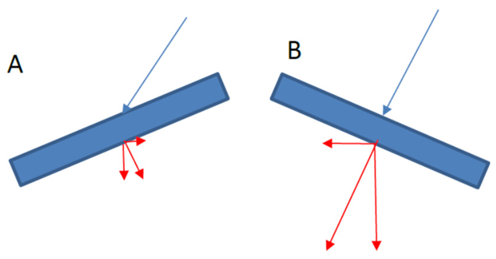
5.2. Wind Wheel Model

We assume that the solar panels of the box wings model are slightly asymmetric, i.e., with a certain canting angle. The canted solar panels are subject to a mechanism similar to that of a wind wheel or fan. As illustrated in Figure 17, the radiation pressure exerts a torque parallel to the axis of the wheel (z axis) and to the incoming radiation.

The motion is more complicated if the incoming radiation is not parallel to the axis of the wheel. If we look at the profiles of the two canted surfaces A and B separately, we see equally distributed forces in Figure 18, while with inclined incident radiation (Figure 19), the forces on A and B are not equal, resulting in an additional torque. In fact, if we imagine another radiation direction aligned with the cylinder axis, we see that the same mechanism applies but with a different torque direction (let us call it transversal torque). Therefore, we can assume that in the general case, both components of the incoming radiation are present and that this will result in two different torques. The transversal torque will force the wind wheel to move away from the ideal orientation in which the light is aligned with the wheel axis. Simulations show this dynamic in Figure 20, where the three axes x, y, z (red, green, blue) in the body-fixed coordinate system are displayed in an inertial system with X, Y, Z axes. The wheel axis corresponds to the z axis and the initial rotation of the wheel is 1°/s. We assume at the simulation epoch, the Sun is pointing in X direction, i.e., parallel to the z direction, and that in the course of the year, the sunlight direction will move in the X-Y plane. At the beginning, the resulting torque causes a rotation around the z axis, which moves the x and y axes in the inertial system (Figure 20). After one month, we have a small variation in the Sun’s direction in the inertial X-Y plane, which will introduce a transversal torque, and the z axis will start to show a precession around the inertial Z axis as illustrated in Figure 21.

The initial rotation velocity is decisive for the spin evolution. Simulations with no initial satellite rotation show an irregular increase in the spin rate, followed by a decrease back to a status with almost no rotation. Figure 22 exhibits the evolution of the angular velocity ${\omega }_z$ about the body-fixed z axis. The explanation of this behavior is related to the precession motion of the satellite previously mentioned. In fact, the satellite changes the orientation during the precession and when the Sun starts to illuminate the back of the “wind wheel” instead of the front part, the opposite rotation is induced. As a consequence, the spin rate decreases and returns to the initial state. Since the precession motion depends on the orientation, the sequence of these cycles is not regular, as can be seen in Figure 22, and tends to have an unpredictable behavior. Simulations with other initial orientations indicate a similar irregular behavior.

The situation is different if the satellite already rotates, e.g., due to outgassing in the initial phase. If the existing angular momentum is large enough, it stabilizes the attitude of the satellite, keeping the orientation of the “wind wheel” approximately constant during the year. The SRP torque contributes essentially to the increase or decrease in the spin rate, without significant changes in the z axis orientation. The amount of spin rate variation depends on the orientation of the wheel in the X-Y plane. The maximal torque occurs with the wheel axis (satellite’s z axis) pointing to the Sun. After 6 months, the maximal effect is obtained in the opposite direction of rotation. The evolution of the angular velocity along the z axis looks as it does in Figure 23, with an initial velocity of 5°/s. A different choice of the initial sunlight direction in the X-Y plane simply shifts the phase of the periodic function. The maximum and minimum of the function are reached during the year when the rotation axis is perpendicular to the Sun’s direction.

If the initial orientation is not in the X-Y plane, no significant changes in the pattern are observed. Only the excursion between maximum and minimum varies according to the optimal orientation of the wheel and the rotational inertia. In fact, the amplitude of the pattern is determined by the inclination of the wind wheel axis with respect to the ecliptic. In case the axis lies in the ecliptic, the maximal amplitude is obtained, while the minimum is reached with a perpendicular axis. The amplitude also varies if the moments of inertia are scaled to larger or smaller values, as well as with higher or lower reflection coefficients or canting angles, with the latter case being consistent with the results in [30]. A behavior similar to the one described above was found by Lips et al. [32] who were analyzing ENVISAT long-term angular velocity simulations. They concluded that when the solar array is illuminated in the spin direction, the SRP torque increases the spin rate. Periodically, the orientation of the solar array with respect to the incoming radiation is flipped, causing an angular acceleration in a counter-spin direction, hence decreasing the rotation velocity.

The yearly variation in the Sun’s position causes a periodic pattern in the angular velocity. However, to obtain a periodic dependency with a secular increasing or decreasing trend, the torque should be smaller/bigger in magnitude during part of the year. This suggests, e.g., to decrease the efficiency of the back side of the “wind wheel”, keeping the front side unchanged. Simulations were performed, setting a specular coefficient of 1 for the front side of the solar panels and 0.5 for the back side. Figure 24 exhibits a secular slope in the angular velocity evolution starting with a 10°/s initial velocity. The same considerations as before apply with different satellite orientations, inertia moments, and canting angles.

In summary, we see the following dependencies in the proposed model:

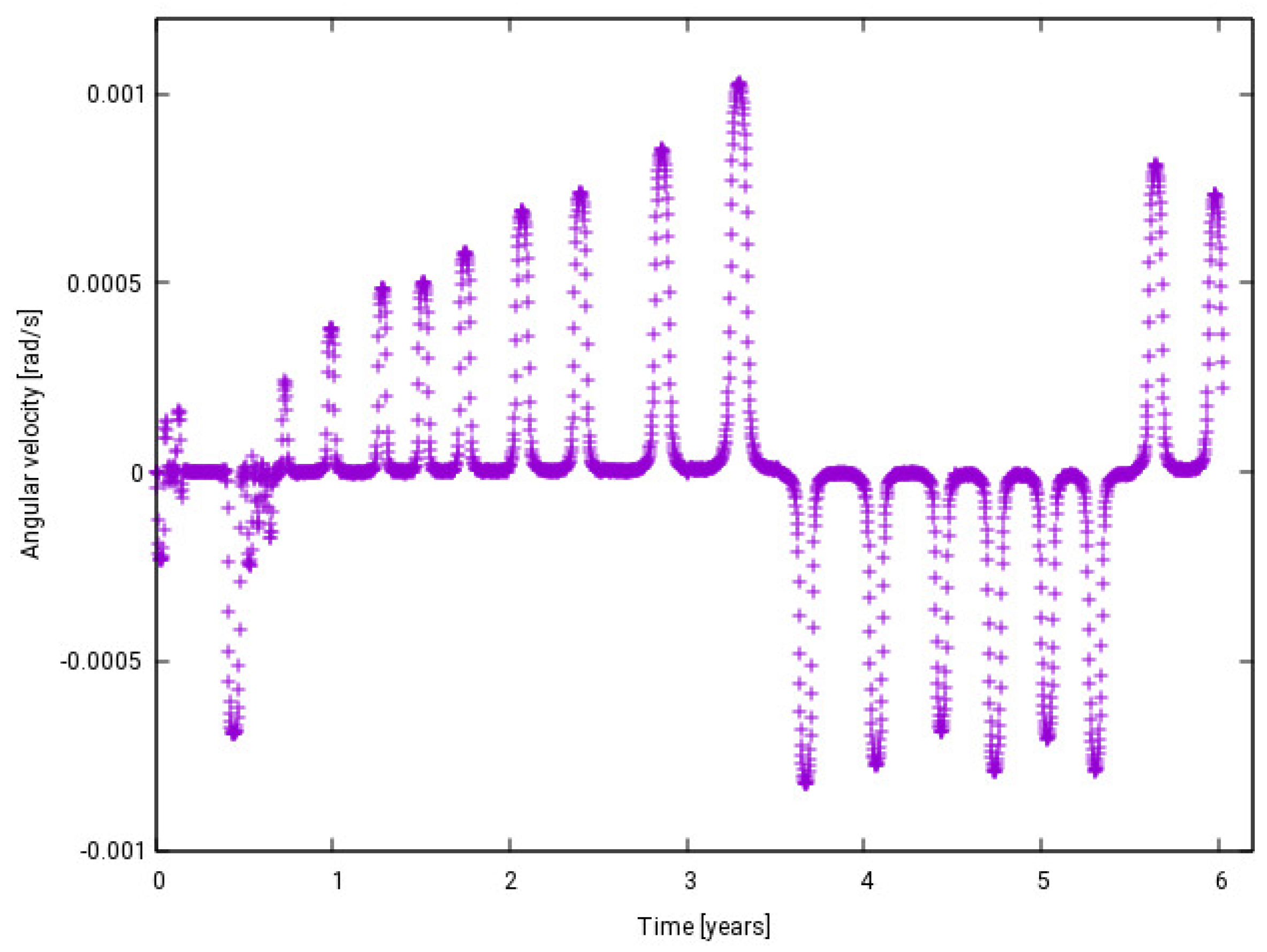
• The initial velocity brings stability in the evolution and the rotation axis keeps its orientation. Simulations with no initial velocity show strong dependence on initial conditions.
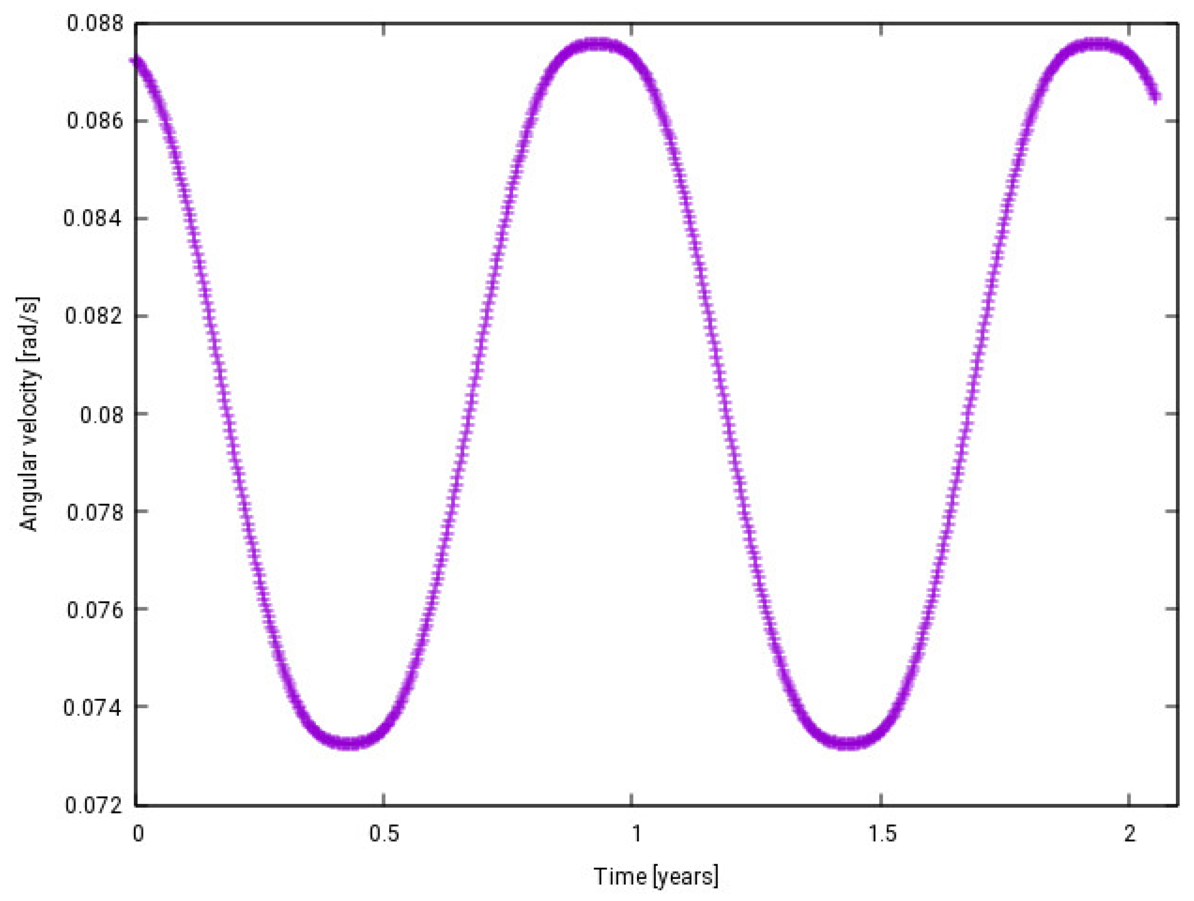
• Through the wind wheel effect, the canting of the panel(s) with a constant orientation of the rotation (wind wheel) axis introduces a periodical variation in the angular velocity related to the position of the Sun during the year.
• The amplitude of the periodical variation is determined by the inclination of the wind wheel axis with respect to the ecliptic. If the axis lies in the ecliptic, the maximal amplitude is obtained. Conversely, the minimum is reached with a perpendicular axis.
• The above amplitude also changes with different canting angles, reflection coefficients, or moments of inertia.
• The phase of the periodical variation depends on the orientation of the wind wheel axis with respect to the Sun’s direction. The maximum and minimum of the periodic curve are reached during the year when the axis is perpendicular to the Sun’s direction.
• Different reflection coefficients for the front/back side of the panels introduce a secular trend in the evolution.

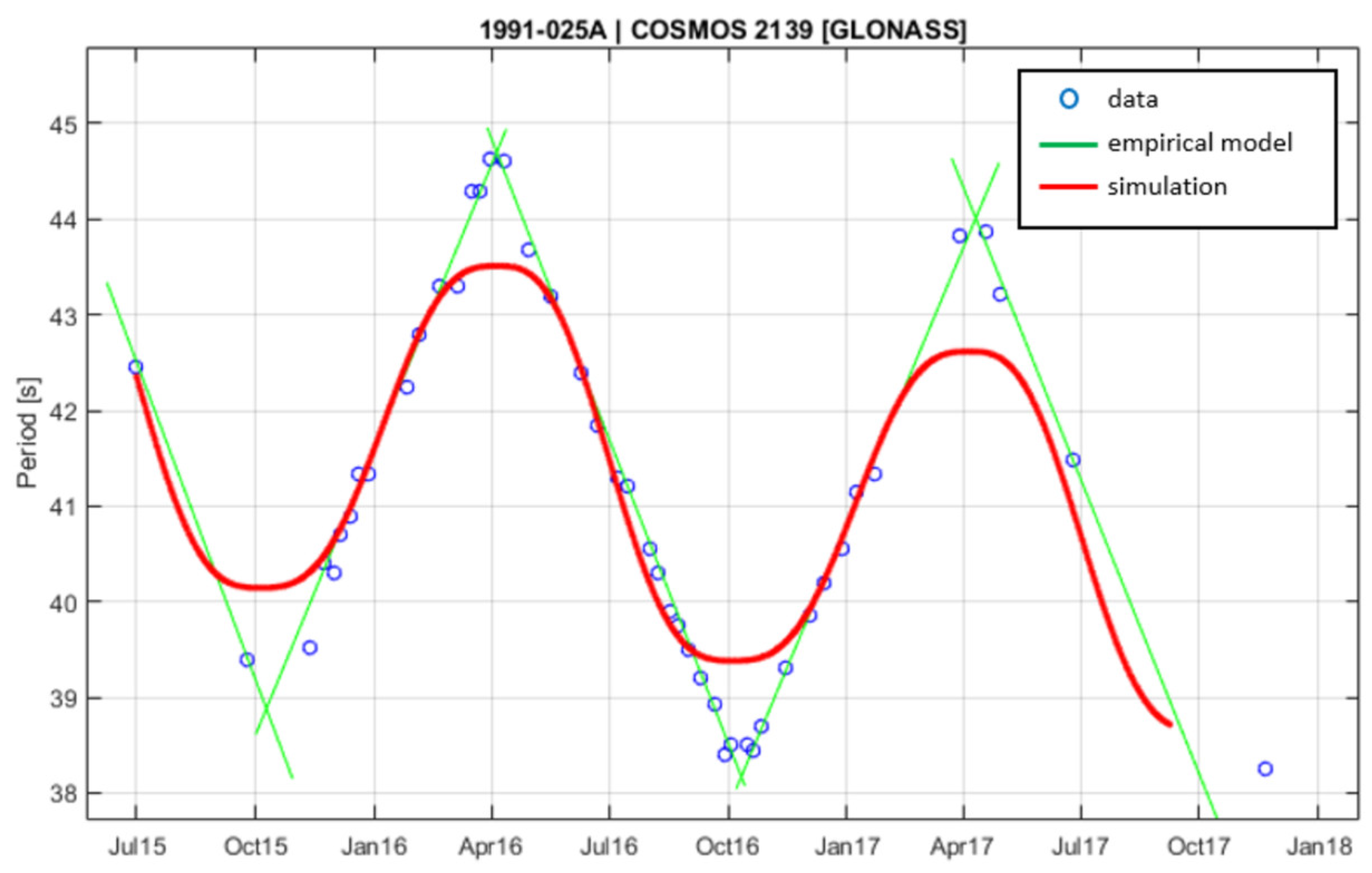
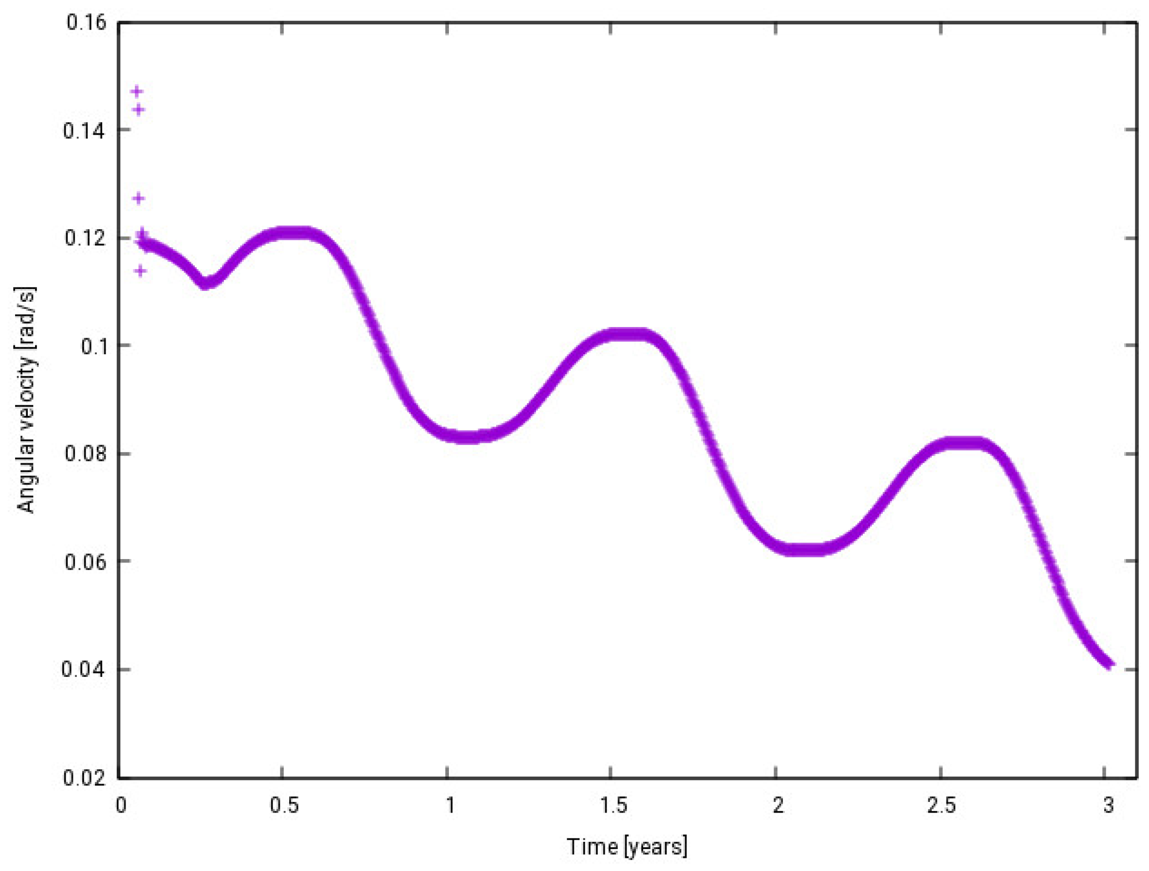
5.3. Simulation of Real Case

Given the above model, it is possible to reproduce the periodic pattern of our selected satellite, COSMOS 2139. According to the mechanism identified above, the following parameters can be changed for fitting purposes:

• The initial velocity shifts the whole plot up or down.
• The direction of the z axis in the ecliptic plane shifts the whole plot left or right (phase of the periodic pattern).
• The value of the specular reflection coefficients determines the amplitude of the plot. In particular, the ratio of the coefficients for the front and back sides of the panels determines the secular slope.
• The canting angle also determines the amplitude in the plot (alternative to the change in reflection coefficients).

In Figure 25, an approximate fit is shown, which was found using the following values:

• Initial velocity: 8.5°/s;
• Direction of z axis in ecliptic plane: 119.3° ecliptic longitude;
• Reflection coefficients, front: 0.5, back: 0.4;
• Canting angle: 5°.

Figure 25. Comparison between observational data and the simulation for COSMOS 2139. Time on the abscissa is indicated in months and years.

Figure 25. Comparison between observational data and the simulation for COSMOS 2139. Time on the abscissa is indicated in months and years.

We notice that periodicity and secular slope can be approximately replicated, but the simulated model is not able to reproduce the sharp observed peaks. In [30], the authors were able to recreate similar peaks using other simulation parameters, but the mechanism behind that specific evolution could not be explained. A factor that was not considered at all in these simulations is the influence of thermal emission from the surfaces of the satellite. This aspect is taken into account in the YORP effect mentioned previously and referred to, e.g., in [24]. This additional component might help better reproduce the observed evolution. Further studies and simulations are necessary to solve this question.

6. Conclusions

This study aims to understand the spin period evolution of some of the inactive GLONASS satellites considered in the AIUB light curve database. More than 1800 light curves for 70 different GLONASS satellites are available in the database. Most of the satellites are first-generation GLONASS (block IIv), while the rest are GLONASS-M satellites. The satellites were launched between 1989 and 2011, and, on average, they had been decommissioned for more than 10 years when first observed by AIUB. Nearly all of them show a rotation behavior and indicate an increase and decrease in spin rate over a certain time interval in addition to an ascending or descending long-term secular trend. Three inactive GLONASS satellites cycle between phases of uniform rotation and a more complex tumbling motion, similarly to the behavior of some GEO satellites under the influence of the YORP effect reported in the literature. In particular, there are 18 satellites that maintain an oscillating pattern with a clear triangular shape over the cataloged period.

The acquired light curves of the cataloged GLONASS satellites typically exhibit four peaks (bright reflections) within a rotation period, in particular, as two pairs of roughly similarly shaped (typically sharp) but differently sized curves. Within the pair, the distance between the peaks is usually around half a period. This morphology can be explained by assuming that the peaks are caused by the four thermal control flaps or radiators, which are distributed evenly around the satellite bus.

The characterization of the oscillating pattern was performed assuming a series of triangular peaks defined by left and right segments with similar slopes. According to this model, the amplitude and period of the oscillations, as well as the secular slope of the pattern, were defined. We found that the average spin period of the objects ranges from 8.11 s to 469.58 s, and this correlates with the average cycle amplitude. The average cycle period ranges from 285.10 days to 494.22 days, and its mean and median values are close to 1 year. Interestingly, we found that, overall, the objects tend to rotate faster during their lifetime, and objects with higher spin rates tend to have a higher angular acceleration.

The regularity of the oscillating pattern allows us to use the empirical model to extrapolate the spin period into the future, assuming that the pattern is preserved with a linear trend, as was the case for six satellites. Others deviated from the linear trend, which may indicate that particular events occurred.

From the simulations of the spin period evolution, we found that the roughly annual oscillating pattern is achievable only if the solar panels are oriented differently, with a certain canting angle, which provides an asymmetry to the satellite model. The assumption that the only force responsible for the oscillating pattern is the SRP was sufficient to reproduce the periodicity of the evolution. The canted solar panels allow a mechanism similar to a wind wheel or fan to work on the system. Depending on the relative orientation of incoming radiation and the axis of rotation, SRP produces a torque on each of the solar panels, resulting in an increase or decrease in the spin rate. When the orientation of the solar panels with respect to the incoming radiation flips after roughly half a year, as the Earth is revolving around the Sun, the angular acceleration changes in a counter-spin direction, decreasing the rotation velocity. The amplitude of the oscillation is determined by the canting angle of the panels and by their reflection coefficients. The secular trend accompanying the spin period oscillation can be obtained as a result of different values of the specular reflection coefficients of the front and back sides of the solar panels. However, the simulations were not able to reproduce the sharp peaks of the observed triangular oscillation pattern. This means that a deeper investigation of the mechanism is still needed, taking into account further factors, like, e.g., thermal emission from the satellite surfaces and the related YORP effect. Additional information about the attitude state of the satellites at different stages of the period evolution would significantly help confirm the proposed model or explore other solutions. The proposed interpretation of the light curves with two pairs of intensity peaks, if confirmed, could also contribute to a better knowledge of the attitude motion. This aspect shall be further investigated with more observations and light curve simulations. Complementary to light curves, since GLONASS satellites are equipped with retroreflectors, laser ranging could provide further data relevant for attitude determination.

References

1. Earl, M.A.; Wade, G.A. Observations and analysis of the apparent spin period variations of inactive boxwing geosynchronous resident space objects. In Proceedings of the 65th International Astronautical Congress, Toronto, ON, Canada, 29 September–3 October 2014. [Google Scholar]
2. Silha, J.; Pittet, J.N.; Hamara, M.; Schildknecht, T. Apparent rotation properties of space debris extracted from photometric measurements. Adv. Space Res. 2018, 61, 844–861. [Google Scholar]
3. Silha, J.; Krajcovic, S.; Zigo, M.; Toth, J.; Zilkova, D.; Zigo, P.; Kornos, L.; Simon, J.; Schildknecht, T.; Cordelli, E.; et al. Space debris observations with the Slovak AGO70 telescope: Astrometry and light curves. Adv. Space Res. 2020, 65, 2018–2035. [Google Scholar]
4. Santoni, F.; Cordelli, E.; Piergentili, F. Determination of disposed-upper-stage attitude motion by ground-based optical observations. J. Spacecr. Rocket. 2013, 50, 701–708. [Google Scholar] [CrossRef]
5. Yanagisawa, T.; Kurosaki, H. Shape and motion estimate of LEO debris using light curves. Adv. Space Res. 2012, 50, 136–145. [Google Scholar] [CrossRef]
6. Zhao, S.; Steindorfer, M.; Kirchner, G.; Zheng, Y.; Koidl, F.; Wang, P.; Shang, W.; Zhang, J.; Li, T. Attitude analysis of space debris using SLR and light curve data measured with single-photon detector. Adv. Space Res. 2020, 65, 1518–1527. [Google Scholar] [CrossRef]
7. Vananti, A.; Lu, Y.; Schildknecht, T. Attitude estimation of H2A rocket body from light curve measurements. Int. J. Astrophys. Space Sci. 2023, 11, 15–22. [Google Scholar] [CrossRef]
8. Nussbaum, M.; Schafer, E.; Yoon, Z.; Keil, D.; Stoll, E. Spectral light curve simulation for parameter estimation from space debris. Aerospace 2022, 9, 403. [Google Scholar] [CrossRef]
9. Vasile, M.; Walker, L.; Dunphy, R.D.; Zabalza, J.; Murray, P.; Marshall, S.; Savitski, V. Intelligent characterisation of space objects with hyperspectral imaging. Acta Astronaut. 2023, 203, 510–534. [Google Scholar]
10. Rachman, A.; Schildknecht, T.; Silha, J.; Pittet, J.N.; Vananti, A. Attitude state evolution of space debris determined from optical light curve observations. In Proceedings of the 68th International Astronautical Congress, Adelaide, Australia, 25–29 September 2017. [Google Scholar]
11. Rachman, A.; Schildknecht, T.; Vananti, A. Analysis of temporal evolution of debris objects’ rotation rates inside AIUB light curve database. In Proceedings of the 69th International Astronautical Congress, Bremen, Germany, 1–5 October 2018. [Google Scholar]
12. Lee, J.; Park, E.; Choi, M.S.; Kucharski, D.; Yi, Y.; Park, J.U. Spin axis determination of defunct GLONASS satellites using photometry observation. J. Astron. Space Sci. 2021, 38, 45–53. [Google Scholar]
13. Albuja, A.; Scheeres, D.J. Defunct satellites, rotation rates and the YORP effect. In Proceedings of the 14th AMOS Technical Conference, Maui, HI, USA, 10–13 September 2013. [Google Scholar]
14. Earl, M.A. Photometric analysis and attitude estimation of inactive boxwing geosynchronous satellites. Ph.D. Thesis, Royal Military College of Canada, Kingston, ON, Canada, 2017. [Google Scholar]
15. Benson, C.; Scheeres, D.J.; Ryan, W.H.; Ryan, E.V.; Moskovitz, N. Rotation state evolution of retired geosynchronous satellites. In Proceedings of the 18th AMOS Technical Conference, Maui, HI, USA, 19–22 September 2017. [Google Scholar]
16. Pittet, J.N.; Šilha, J.; Schildknecht, T. Spin motion determination of the Envisat satellite through laser ranging measurements from a single pass measured by a single station. Adv. Space Res. 2018, 61, 1121–1131. [Google Scholar] [CrossRef]
17. Kirchner, G.; Steindorfer, M.; Wang, P.; Koidl, F.; Kucharski, D.; Silha, J.; Schildknecht, T.; Krag, H.; Flohrer, T. Determination of attitude and attitude motion of space debris, using laser ranging and single-photon light curve data. In Proceedings of the 7th European Conference on Space Debris, Darmstadt, Germany, 18–21 April 2017. [Google Scholar]
18. Silha, J.; Schildknecht, T.; Pittet, J.N.; Kirchner, G.; Steindorfer, M.; Kucharski, D.; Cerutti-Maori, D.; Rosebrock, J.; Sommer, S.; Leushacke, L.; et al. Debris attitude motion measurements and modelling by combining different observation techniques. J. Br. Interplanet. Soc. 2017, 70, 52–62. [Google Scholar]
19. Pontieu, B.D. Database of photometric periods of artificial satellites. Adv. Space Res. 1997, 19, 229–232. [Google Scholar] [CrossRef]
20. Albuja, A.A.; Scheeres, D.J.; McMahon, J.W. Evolution of angular velocity for defunct satellites as a result of YORP: An initial study. Adv. Space Res. 2015, 56, 237–251. [Google Scholar] [CrossRef]
21. Ojakangas, G.W.; Hill, N. Toward realistic dynamics of rotating orbital debris and implications for light curve. In Proceedings of the 12th AMOS Technical Conference, Maui, HI, USA, 13–16 September 2011. [Google Scholar]
22. Albuja, A.A.; Scheeres, D.J.; Cognion, R.L.; Ryan, W.; Ryan, E.V. The YORP effect on the GOES 8 and GOES 10 satellites: A case study. Adv. Space Res. 2018, 61, 122–144. [Google Scholar] [CrossRef]
23. Benson, C.J.; Scheeres, D.J.; Ryan, W.H.; Ryan, E.V. Cyclic complex spin state evolution of defunct GEO satellites. In Proceedings of the 19th AMOS Technical Conference, Maui, HI, USA, 11–14 September 2018. [Google Scholar]
24. Benson, C.J.; Scheeres, D.J.; Ryan, W.H.; Ryan, E.V.; Moskovitz, N.A. GOES spin state diversity and the implications for GEO debris mitigation. Acta Astronaut. 2020, 167, 212–221. [Google Scholar] [CrossRef]
25. Revnivykh, S.; Bolkunov, A.; Serdyukov, A.; Montenbruck, O. GLONASS. In Springer Handbook of Global Navigation Satellite Systems; Teunissen, P.J.G., Montenbruck, O., Eds.; Springer: Cham, Switzerland, 2017. [Google Scholar]
26. Linder, E.; Silha, J.; Schildknecht, T.; Hager, M. Extraction of spin periods of space debris from optical light curves. In Proceedings of the 66th International Astronautical Congress, Jerusalem, Israel, 12–16 October 2015. [Google Scholar]
27. Earl, M.A.; Somers, P.W.; Kabin, K.; Bedard, D.; Wade, G.A. Estimating the spin axis orientation of the Echostar-2 box-wing geosynchronous satellite. Adv. Space Res. 2018, 61, 2135–2146. [Google Scholar] [CrossRef]
28. Kanzler, R.; Silha, J.; Schildknecht, T.; Fritsche, B.; Lips, T.; Krag, H. Space debris attitude simulation-iOTA (In-Orbit Tumbling Analysis). In Proceedings of the 15th AMOS Technical Conference, Maui, HI, USA, 9–12 September 2014. [Google Scholar]
29. Sagnieres, L.B.M.; Sharf, I.; Deleflie, F. Simulation of long-term rotational dynamics of large space debris: A TOPEX/Poseidon case study. Adv. Space Res. 2020, 65, 1182–1195. [Google Scholar]
30. Rachman, A.; Vananti, A.; Schildknecht, T. Understanding the oscillating pattern in the rotational period evolution of several GLONASS satellites. In Proceedings of the 21st AMOS Technical Conference, Maui, HI, USA, 14–18 September 2020. [Google Scholar]
31. Wertz, J.R. Spacecraft Attitude Determination and Control; Astrophysics and Space Science Library; Kluwer Academic Publishers: Dordrecht, The Netherlands, 1978; Volume 73. [Google Scholar]
32. Lips, T.; Kanzler, R.; Breslau, A.; Kärräng, P.; Silha, J.; Schildknecht, T.; Kucharski, D.; Kirchner, G.; Rosebrock, J.; Cerutti-Maori, D.; et al. Debris attitude motion measurements and modelling observation vs. simulation. In Proceedings of the 18th AMOS Technical Conference, Maui, HI, USA, 19–22 September 2017. [Google Scholar]
Figure 1. Example of a light curve measured at AIUB.
Aerospace 12 00283 g001
Figure 2. Phase diagram for the light curve in Figure 1 with a period of 210.65 ± 0.1 s.
Aerospace 12 00283 g002
Figure 3. Example of GLONASS stable light curve.
Aerospace 12 00283 g003
Figure 4. Example of GLONASS slow-changing light curve.
Aerospace 12 00283 g004
Figure 5. An example of a spin period evolution of GLONASS satellites. Time on the abscissa is indicated in months and years.
Aerospace 12 00283 g005
Figure 6. Spin period evolution of COSMOS 2236. Red circles indicate extracted periods. Lines refer to light curves in which the period could not be determined, such as in the case of slow-changing light curves (black) or a complex non-repeating pattern (green). Time on the abscissa is indicated in years.
Aerospace 12 00283 g006
Figure 7. Spin period evolution of COSMOS 2275. Red circles indicate extracted periods. Lines refer to light curves in which the period could not be determined, such as in the case of slow-changing light curves (black) or a complex non-repeating pattern (green). Time on the abscissa is indicated in years.
Aerospace 12 00283 g007
Figure 8. Spin period evolution of COSMOS 2411. Red circles indicate extracted periods. Black lines refer to slow-changing light curves. Time on the abscissa is indicated in years.
Aerospace 12 00283 g008
Figure 9. Different examples in (ad) of phase diagrams of inactive GLONASS satellites. They typically show four peaks in two pairs. The two pairs are identified by two arcs of different colors.
Aerospace 12 00283 g009aAerospace 12 00283 g009bAerospace 12 00283 g009c
Figure 10. A simplified scenario to explain the presence of two pairs of peaks. The bus is looked at from one end. The four radiators are marked with numbers. In this illustration, the bus is rotating clockwise around its minimum axis of inertia. P is the spin period of the satellite.
Aerospace 12 00283 g010
Figure 11. Basic model of spin period evolution. a, b, and c are parameters within the triangular shape that are used in characterizing the empirical model of a specific object.
Aerospace 12 00283 g011
Figure 12. Spin period evolution according to observational data (left) and empirical model (right) for a sample object. The red line runs through the centers of the applicable segments to represent the average dynamics of the evolution. Each segment is labeled with a number, while red dots represent peaks. Time on the abscissa is indicated in months and years.
Aerospace 12 00283 g012
Figure 13. The observational data (blue circle) and its model (green segments) for the spin period evolution of COSMOS 2139. Each segment is marked with a number. A red cross on the last segment (segment number 11) indicates the period obtained using the model, which matches well with the observation. Time on the abscissa is indicated in months and years.
Aerospace 12 00283 g013
Figure 14. Long-term variation in the average spin period. Cubic splines are used to represent the average dynamics of the evolution. COSPAR ID and the reference object’s number in Table 2 are indicated. Time on the abscissa uses the notation mm (month) and yy (year).
Aerospace 12 00283 g014
Figure 15. Relationship between average cycle amplitude and average spin period of the objects.
Aerospace 12 00283 g015
Figure 16. Relationship between the average secular trend and average spin period of the objects.
Aerospace 12 00283 g016
Figure 17. Scheme of radiation pressure for canted surfaces and resulting torque parallel to the z axis. The vectors n ^ A , B normal to the surfaces and the vectors N A , B related to the projected sunlight direction are indicated.
Aerospace 12 00283 g017
Figure 18. Profile view of resulting forces on canted surfaces (A,B). Radiation parallel to wheel axis.
Aerospace 12 00283 g018
Figure 19. Profile view of resulting forces on canted surfaces (A,B). Radiation not parallel to wheel axis.
Aerospace 12 00283 g019
Figure 20. Initial attitude motion of the object with rotation about the wheel axis (blue vector). The red, green, blue vectors represent the three axes x, y, z in the body-fixed coordinate system, while the X, Y, Z axes define the inertial system. Red and green vectors indicate the rotation, moving from one position (left) to a rotated one (right).
Aerospace 12 00283 g020
Figure 21. Precession of the wheel axis (blue vector) around the Z axis under transversal torque. The blue vector moves from one direction (left) to a slightly different one (right), remaining on the X-Y plane, while red and green vectors indicate the rotation about the wheel axis.
Aerospace 12 00283 g021
Figure 22. Angular velocity as a function of time for the case with no initial rotation.
Aerospace 12 00283 g022
Figure 23. Angular velocity as a function of time for the case with initial rotation.
Aerospace 12 00283 g023
Figure 24. Angular velocity as a function of time in the case with different optical properties for the front and back sides of the solar panels.
Aerospace 12 00283 g024