Slot Allocation for a Multi-Airport System Considering Slot Execution Uncertainty

Abstract

Capacity–flow balance constitutes the primary challenge in strategic slot allocation. Both air traffic flow and airport flow are significantly influenced by departure/arrival times of flights. However, due to various uncontrollable factors such as flow control, delay propagation, and weather conditions, the actual departure/arrival times of flights inevitably deviate from their schedules. This reflects the inherent uncertainty in flight slot execution, which directly introduces uncertainty into capacity–flow analysis. In this paper, we develop an uncertainty slot allocation model for the multi-airport system (MAS), which incorporates slot execution deviation as an uncertainty factor with fix capacity restrictions formulated as chance constraints to balance robustness and optimality. To solve the model, we employ an equivalent model transformation approach and develop a scenario generation methodology. We applied our model to the MAS of Beijing–Tianjin for slot allocation. The results show that when the violation probability $\alpha \in [0,0.2]$ , the model achieved fully robust optimization. Even when $\alpha$ increases to 0.4, under all scenario combinations, at the selected fix, compared with the results of the deterministic model and original schedules, the number of peak flow time windows in the expected traffic statistics decreased by 84.6% and 75%, respectively, and the average maximum values of traffic in the maximum traffic statistics decreased by 31.1% and 33.5%, respectively. Furthermore, the incorporation of the chance constraint provides slot coordinators with flexible optimization solutions based on their acceptable risk levels.

1. Introduction

Scientific and rational slot allocation can effectively balance capacity with flight flow, optimize airspace resource utilization, and consequently alleviate congestion and delay issues. The Worldwide Slots Guidelines (WSG) published by IATA (International Air Transport Association) defines a slot as “A scheduled operational permission granted by the coordinator, allowing the use of all necessary airport infrastructure for arrival or departure at a Level 3 (coordinated) airport on a specific date and time” [1]. China’s “Civil Aviation Flight Slot Management Regulations” define a slot as “the right to use relevant infrastructure and services at a designated airport for aircraft arrival or departure on specified dates and times”. It further specifies that the slot for an arriving flight is the block-on time, while for a departing flight it is the block-off time [2].

Initial slot allocation research focused on single airports. In the early 2000s, Hu et al. developed a multi-constrained slot optimization model based on ground holding strategies tailored to China’s airspace operations and slot allocation characteristics, along with an improved heuristic algorithm [3]. In 2012, Zografos et al. formulated the single-airport slot optimization problem as an integer programming model [4], incorporating IATA WSG and EU 95/93 regulations, airport capacity constraints, turnaround time limits, and priority groups for slot requests, aiming to minimize scheduled delays. Their results demonstrated significant reductions in airline “schedule-induced delay”. Subsequently, slot allocation models evolved from single-objective to multi-objective optimization [5], expanding beyond total displacement minimization to include minimizing maximum displacement, reducing out-of-window slots, and enhancing fairness. Notable contributions include Zografos et al.’s 2018 dual-objective models, which balanced allocation efficiency and slot acceptability [6], and later work incorporating fairness [7,8]. These studies showed that minor sacrifices in coordination efficiency could significantly improve other metrics. Ribeiro’s models further integrated IATA rules and their complex priority structures [9,10,11]. For the allocation of newly added slots, Wang et al. optimized incremental slot resources at single airports by considering key resource node capacities and flight waves, aligning strategic and tactical optimization [12]. Some researchers have also studied the value of the slot from the perspective of airlines. Cao et al. used a minimum cost flow model to analyze the impact of slot reassignment on airline profits, quantifying the value of runway time and calculating the optimal slot allocation under runway capacity constraints [13]. Olbrich et al. evaluated the value of the slot using a subjective value approach combined with discounted cash flow (DCF) models and linear programming models to assist airlines in optimizing slot resource investment decisions in markets with excess demand [14].

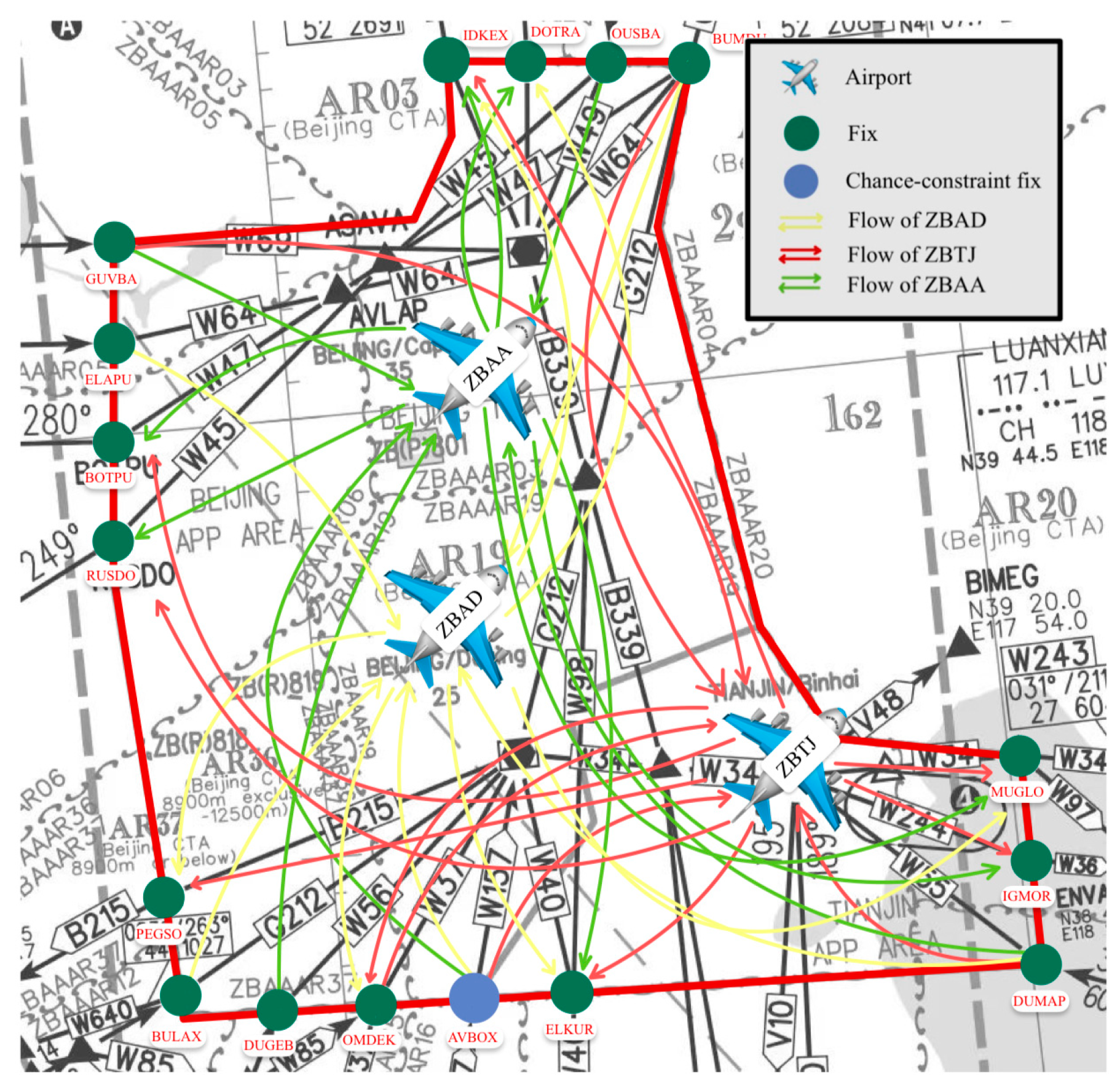
With the increasing regional economic integration, the collaborative role among airports has become more pronounced. Geographically proximate airports have gradually formed multi-airport systems (MASs). Research on MASs began in 2008 when the Joint Planning and Development Office (JPDO) first defined a MAS as a group of airports serving a region [15]. These airports are geographically close, interdependent in their arrival/departure routes, and form a metroplex (a combination of metropolitan and complex). For instance, the MAS of Beijing–Tianjin (Figure 1) includes major airports such as Beijing Capital International Airport (ICAO code: ZBAA), Beijing Daxing International Airport (ICAO code: ZBAD), and Tianjin Binhai International Airport (ICAO code: ZBTJ) within the terminal airspace provided by three air traffic control departments: Beijing Approach Control, Daxing Approach Control, and Tianjin Approach Control. With the rapid growth of air transport demand, the interdependence and constraints among MAS airports have become increasingly evident, particularly in shared airspace resources. Such conflicts are primarily manifested in commonly used arrival/departure fixes and routes, intensifying competition for airspace resources. As the need for coordinated operations in MASs grows more urgent, researchers have recognized the limitations of traditional single-airport slot optimization models and begun exploring coordinated slot optimization methods at the MAS and airport network levels. Castelli, Pellegrini, and others proposed an airport network slot allocation model [16,17], which considers sector capacity constraints and aims to minimize slot displacements resulting from inconsistencies between the slot allocations at the origin and destination airports. Corolli et al. further incorporated airport capacity uncertainty, developing a two-stage stochastic programming model [18]. The primary challenge in MAS slot allocation lies in model solving, as the variable and constraint scales are often excessively large. Various solution algorithms have been applied, including heuristic algorithms [19], intelligent optimization algorithms [20], and dual integer cutting methods [21].

In recent studies, Wang et al. proposed a low-carbon flight slot allocation model integrated with a variable neighborhood search algorithm, achieving a 26.3% reduction in carbon emissions while maintaining comparable flight delay levels [22]. Melder et al. and Katsigiannis et al. addressed airport congestion by employing integer linear programming combined with heuristic algorithms and a multi-objective Operations Research–Machine Learning (OR-ML) hybrid framework, respectively, to optimize resource allocation and mitigate blocking issues [23,24]. Zeng et al. enhanced the Worldwide Slot Guidelines by introducing a dual-objective model with operational priority, reducing slot adjustments to 3.15% and improving spatiotemporal scheduling rationality [25]. Berktas et al. developed a generic mixed-integer linear programming model applicable across airports, ports, and rail systems, demonstrating its efficiency in railway scheduling and providing a unified methodology for multi-modal terminal capacity allocation [26].

Strategic-level slot allocation is inherently a resource-constrained assignment problem. Airport capacity is limited by factors such as runway availability, gate configurations, ground handling capabilities, and weather conditions. Similarly, airspace capacity is constrained by airspace structure, ATC regulations, and separation standards. Fixes, as critical nodes for terminal area access, significantly influence airspace utilization efficiency through their capacity–flow matching performance. Airport flow can be estimated by counting flights within specific time windows based on flights’ departure/arrival times, while fix flow requires additional consideration of flying times between airports and fixes. Both flow calculations are subject to uncertainty because the actual departure/arrival times inevitably deviate from their schedules due to the inherent complexity of air transport systems and various uncontrollable factors. This slot execution uncertainty directly leads to flow uncertainty, thereby posing significant challenges for MAS slot allocation.

Stochastic programming and the chance constraint are regarded as promising approaches to handling uncertainty in numerous fields [27]. Geletu A et al. provide a detailed overview of these applications [28]. Recently, some researchers have combined machine learning with chance constraints: building on constraint learning [29], they integrate chance constraints to effectively address the inherent uncertainty of point prediction models [30]. Stochastic programming (SP), with its relatively simple model structure, has seen extensive use in uncertain optimization tasks such as vehicle routing [31], capacity expansion [32], and production scheduling [33]. In the field of slot allocation, two-stage SP models have been employed to capture airport capacity uncertainties [18,21,34]. Stochastic programming is also an effective tool for solving chance constraints, which are transformed in this paper into deterministic constraints based on the theory to complete the model solution. In addition, SP has been applied to ATFM [35], airport congestion management [36], and tactical aircraft sequencing in ATM [37,38,39]. Current research on slot allocation under uncertainty largely focuses on capacity uncertainty, while demand uncertainty, i.e., flow uncertainty, has received less attention. Liu et al. developed a slot optimization model incorporating flying time uncertainty, significantly enhancing the robustness of strategic schedules through reallocation in the Guangdong–Hong Kong–Macao Greater Bay Area MAS [40]. However, few studies have integrated execution uncertainty into slot allocation models.

To address this issue, we first propose a certainty slot allocation model (CSAM) and then develop an uncertainty slot allocation model (USAM) that incorporates slot execution uncertainty. To explore the balance between optimality and robustness, we formulate fix capacity constraints as chance constraints in the USAM. Using stochastic programming methods, we transform the USAM into a converted uncertainty slot allocation model (CUSAM) suitable for solver implementation. Additionally, we construct a scenario generation model (SGM), whose outputs are utilized in solving the USAM. Finally, we validate the model using operational data from the MAS of Beijing–Tianjin.

The remainder of this paper is organized as follows: Section 2 details the development of the CSAM and USAM, along with a solution approach that transforms the USAM into CUSAM for direct solving using the Gurobi solver. Additionally, this section presents the scenario generation methodology through the construction of the GSM. Section 3 describes the numerical experiments and analyzes the results. Finally, Section 4 summarizes the main findings and provides recommendations for future research.

2. Model

2.1. Model Description

To facilitate modeling and discussion, we establish the following assumptions:

• Slots in this study represent small time windows rather than precise time points, with a 5 min duration in the model.
• The cost per unit adjustment is identical for all flights.
• Only arrival/departure flights within the MAS are considered, excluding overflights.
• Slot execution deviations for arrival/departure flights within 24 hourly time windows across days in historical data are mutually independent. The scenario generation model produces experimental scenarios with independent probability distributions.
• Flight cancellations are not considered during the slot allocation.

The model inputs include the following: (i) strategic schedules for each airport in the MAS, containing the flight number, aircraft registration, departure/arrival times, origin/destination airports, and flight routes for each flight; (ii) capacity limits for each airport and fix in the MAS; (iii) flying times between airports and fixes in the MAS; (iv) minimum and maximum turnaround times for connecting flights; and (v) slot execution deviation scenarios and their occurrence probabilities for each airport. The strategic schedules are obtained from airports. Airport–fix flying times, airport capacities, and fix capacities are provided by air traffic control authorities, with capacities given as envelope curves. Minimum and maximum turnaround times are set according to national or airport regulations. Slot execution deviation scenarios and their probabilities are calculated by the SGM, which is detailed in Section 2.5. The output is the optimized flight schedule. The objective function minimizes the total slot displacement across all flights to reduce strategic allocation costs. During the modeling process, we first establish a CSAM, then introduce slot execution deviation as an uncertainty parameter, while transforming fix capacity constraints into chance-constrained formulations to obtain the USAM.

Table 1. Model notation and description.

Notation	Description
Sets
$T$	$\mathrm{Set} \mathrm{of} \mathrm{slots} \mathrm{within} \mathrm{a} \mathrm{day}, n=1,2,3\dots \in T$
$D_w$	$\mathrm{Set} \mathrm{of} \mathrm{time} \mathrm{windows} \mathrm{within} \mathrm{a} \mathrm{day}, w=1,2,3\dots \in D_w$
$T_w$	Set of slots within time window $w$
$A_k$	Set of slot execution deviation scenario indices for airport $k$, $a_k=1,2,3\dots \in A_k$
$K$	Set of airports within the MAS
$F$	Set of flights within the MAS
$Q$	Set of fixes within the MAS
$F_c$	Set of connecting flights
$F^{\mathrm{arr}}/F^{dep}$	Set of arrival/departure flights within the MAS
$F_k^{arr}/F_k^{dep}$	Set of arrival/departure flights for airport $k$$, k\in K$
$F_q^{arr}/F_q^{dep}$	Set of arrival/departure flights passing fix $q$$, q\in Q$
Parameters
$t_e$	The latest slot within a day to which a flight can be adjusted
$A$	Number of slot execution deviation scenarios for an airport
$C_m/C_M$	Minimum/maximum turnaround time for connecting flights
${\mathsf{\Delta }}_M$	Maximum slot adjustment for each flight
$a_k$	Slot execution deviation scenario index for airport $k$$, a_k\in A$
$O_{i,n}^{arr}/O_{i,n}^{dep}$	Binary parameter, where 1 indicates that flight $i$ is scheduled to arrive or depart no earlier than slot $n$  $\mathrm{in} \mathrm{the} \mathrm{original} \mathrm{schedule}, \mathrm{and} 0 \mathrm{otherwise}, i\in F,n\in T$
$C_k^{arr}/C_k^{dep}/C_k^{all}$	Declared airport capacity, representing the maximum number of flights that can arrive/depart/arrive and depart at airport $k$ within time window $w$$, k\in K,w\in D_W$
$C_q$	Declared fix capacity, representing the maximum number of flights that can pass fix $q$ within time window $w$$, q\in Q,w\in T_w$
$f_{k,q}^{\mathrm{arr}}/f_{k,q}^{dep}$	Flying time between airport $k$ and fix $q$$\mathrm{for} \mathrm{arrival}/\mathrm{departure} \mathrm{flights}, k\in K,q\in Q$
${\mathsf{\Delta }}_{i,n,k}^{arr}/{\mathsf{\Delta }}_{i,n,k}^{dep}$	Random parameter representing the slot execution deviation for arrival/departure flight $i$ at airport $k$ scheduled at slot $n$$, i\in F,n\in T,k\in K$
${\mathsf{\Delta }}_{i,n,k}^{arr(a_k)}/{\mathsf{\Delta }}_{i,n,k}^{dep(a_k)}$	Slot execution deviation for arrival/departure flight $i$ scheduled at slot $n n$ at airport $k$ under scenario $a_k$$, i\in F,n\in T,k\in K,a_k\in A$
$p_k^{arr(a_k)}/p_k^{dep(a_k)}$	$\mathrm{Probability} \mathrm{of} \mathrm{slot} \mathrm{execution} \mathrm{deviation} \mathrm{scenario} a_k$ occurring at airport $k$$, k\in K,a_k\in A$
$\alpha$	Violation probability in chance constraints
Decision variables
$x_{i,n}^{\mathrm{arr}}/x_{i,n}^{\mathrm{dep}}$	Binary decision variable, where 1 indicates that flight $i$ is scheduled to arrive or depart no earlier than slot $n$$\mathrm{in} \mathrm{the} \mathrm{optimized} \mathrm{schedule}, \mathrm{and} 0 \mathrm{otherwise}, i\in F,n\in T$
$y_{i,n,k}^{arr(a_k)}/y_{i,n,k}^{dep(a_k)}$	Binary decision variable, where 1 indicates that flight $i$ is scheduled to arrive or depart no earlier than slot $k$$\mathrm{in} \mathrm{the} \mathrm{optimized} \mathrm{schedule}, \mathrm{under} \mathrm{slot} \mathrm{execution} \mathrm{deviation} \mathrm{scenario} a_k$, arrives or departs no earlier than slot $n$, and 0 otherwise $, i\in F,n\in T,a_k\in A,k\in K$
Indirect decision variables
${\gamma }_{k,q,n}^{\mathrm{arr}}/{\gamma }_{k,q,n}^{\mathrm{dep}}$	Number of flights scheduled to arrive or depart at slot $n$ at airport $k$ in the optimized schedule that pass fix $q$$, k\in K,q\in Q,n\in T$
${\beta }_{k,q,n}^{\mathrm{arr}(a_k)}/{\beta }_{k,q,n}^{\mathrm{dep}(a_k)}$	Number of flights arriving/departing at slot $n$ at airport $k$ in the optimized schedule that pass fix $q$ under slot execution deviation scenario $a_k$, $k\in K,q\in Q,n\in T$

provides the notation description.

2.2. The Certainty Slot Allocation Model (CSAM)

We first formulate a CSAM, which is a mixed-integer programming model (MIPM). The model includes the set of airports $K$, the set of flights $F$, and the set of fixes $Q$ in the MAS. Based on the assumption, we discretize the time of day by treating every 5 min as a slot and assigning a unique index, with the set of slots in a day denoted as $T$. For each arrival/departure flight $i\in F$, we define binary decision variable $x_{i,n}^{\mathrm{arr}}/x_{i,n}^{\mathrm{dep}}$ in the form of (1,1,1,…,1,0,0,0,…,0). $x_{i,n}^{\mathrm{arr}}/x_{i,n}^{\mathrm{dep}}=1$ indicates that flight $i$ is scheduled to arrive or depart no earlier than slot $n$ in the optimized schedule, and 0 otherwise. Thus, we can determine whether flight $i$ arrives/departs at slot $n$ by checking if $x_{i,n}^{arr}-x_{i,n+1}^{arr}=1$ or $x_{i,n}^{dep}-x_{i,n+1}^{dep}=1$. The CSAM can be formulated as follows:

$$Z_a=min\left\{\sum _{n\in T}\sum _{i\in F^{arr}}\left|x_{i,n}^{arr}-O_{i,n}^{arr}\right|+\sum _{n\in T}\sum _{i\in F^{dep}}\left|x_{i,n}^{dep}-O_{i,n}^{dep}\right|\right\}$$

(1)

$$x_{i,1}^{arr}=1,\forall i\in F^{arr}$$

(2)

$$x_{i,t_e}^{arr}=0,\forall i\in F^{arr}$$

(3)

$$x_{i,1}^{dep}=1,\forall i\in F^{dep}$$

(4)

$$x_{i,t_e}^{dep}=0,\forall i\in F^{dep}$$

(5)

$$x_{i,n}^{arr}\ge x_{i,n+1}^{arr},\forall n\in T,\forall i\in F^{arr}$$

(6)

$$x_{i,n}^{dep}\ge x_{i,n+1}^{dep},\forall n\in T,\forall i\in F^{dep}$$

(7)

$$\sum _{n\in T}\left(x_{j,n}^{dep}-x_{i,n}^{arr}\right)\ge C_m,\forall (i,j)\in F_c$$

(8)

$$\sum _{n\in T}\left(x_{j,n}^{dep}-x_{i,n}^{arr}\right)\le C_M,\forall (i,j)\in F_c$$

(9)

$$\sum _{n\in T}|x_{i,n}^{arr}-O_{i,n}^{arr}|\le {\mathsf{\Delta }}_M,\forall i\in F^{arr}$$

(10)

$$\sum _{n\in T}|x_{i,n}^{dep}-O_{i,n}^{dep}|\le {\mathsf{\Delta }}_M,\forall i\in F^{dep}$$

(11)

$$\sum _{n\in T_w}\sum _{i\in F_k^{arr}}\left(x_{i,n}^{arr}-x_{i,n+1}^{arr}\right)\le C_k^{arr},\forall w\in D_w,\forall k\in K$$

(12)

$$\sum _{n\in T_w}\sum _{i\in F_k^{dep}}\left(x_{i,n}^{dep}-x_{i,n+1}^{dep}\right)\le C_k^{dep},\forall w\in D_w,\forall k\in K$$

(13)

$$\sum _{n\in T_w}\sum _{i\in F_k^{arr}}\left(x_{i,n}^{arr}-x_{i,n+1}^{arr}\right)+\sum _{n\in T_w}\sum _{i\in F_k^{dep}}\left(x_{i,n}^{dep}-x_{i,n+1}^{dep}\right)\le C_k^{all},\forall w\in D_w,\forall k\in K$$

(14)

$${\gamma }_{k,q,n}^{arr}=\sum _{i\in F_k^{arr}\cap F_q^{arr}}\left(x_{i,n}^{arr}-x_{i,n+1}^{arr}\right),\forall k\in K,\forall q\in Q,\forall n\in T$$

(15)

$${\gamma }_{k,q,n}^{dep}=\sum _{i\in F_k^{dep}\cap F_q^{dep}}\left(x_{i,n}^{dep}-x_{i,n+1}^{dep}\right),\forall k\in K,\forall q\in Q,\forall n\in T$$

(16)

$$\sum _{n\in T_W}\sum _{k\in K}{\gamma }_{k,q,n+f_{k,q}^{arr}}^{arr}+\sum _{n\in T_W}\sum _{k\in K}{\gamma }_{k,q,n-f_{k,q}^{dep}}^{dep}\le C_q,\forall w\in D_w,\forall q\in Q$$

(17)

Equation (1) represents the objective function, aiming to minimize the total flight slot displacement, where ${\displaystyle \sum _{n\in T}}\left|x_{i,n}^{arr}-O_{i,n}^{arr}\right|/{\displaystyle \sum _{n\in T}}\left|x_{i,n}^{dep}-O_{i,n}^{dep}\right|$ denotes the slot displacement for arrival/departure flight $i$. Constraints (2)–(5) are flight existence constraints. Based on the assumption, we restrict the decision variables to 1 at the first slot of the day and 0 at the last, ensuring each flight is assigned at least one slot and not canceled. Constraints (6) and (7) are flight uniqueness constraints. By enforcing the non-increasing property of decision variables over time, they ensure that there is at most one slot $n$ where $x_{i,n}^{arr}-x_{i,n+1}^{arr}=1$ or $x_{i,n}^{dep}-x_{i,n+1}^{dep}=1$, guaranteeing that each flight is assigned no more than one slot. Constraints (8) and (9) are connecting flight turnaround constraints. For each connecting flight pair, the interval between the arrival time of the preceding flight and the departure time of the subsequent flight must not be less than the minimum turnaround time nor exceed the maximum turnaround time. Constraints (10) and (11) are maximum acceptable slot displacement constraints, ensuring that all flight adjustments remain within acceptable limits. Equations (12)–(14) represent airport capacity constraints. These three constraints collectively form the airport capacity envelope, limiting arrival/departure flow and total flow at any airport within any time window. The equations provide methods to calculate arrival/departure flow and total flow at airport $k$ within time window $w$. Time window lengths are typically 15 min and 60 min. Equations (15) and (16) provide the calculation method for the flow of flights arriving/departing at slot $n$ at airport $k$ that pass fix $q$. Considering the flying times $f_{k,q}^{arr}/f_{k,q}^{dep}$ between airport $k$ and fix $q$, the arrival/departure flow at fix $q$ within time window $w$ is expressed in Equation (17) as ${\displaystyle \sum _{n\in T_W}}{\displaystyle \sum _{k\in K}}{\gamma }_{k,q,n+f_{k,q}^{arr}}^{arr}/{\displaystyle \sum _{n\in T_W}}{\displaystyle \sum _{k\in K}}{\gamma }_{k,q,n-f_{k,q}^{dep}}^{dep}$. Equation (17) represents fix capacity constraints, ensuring that the flow at any fix within any time window does not exceed its capacity limit.

2.3. The Uncertainty Slot Allocation Model (USAM)

Next, we formulate the USAM considering slot execution uncertainty based on the CSAM. We introduce the slot execution deviation ${\mathsf{\Delta }}_{i,n,k}^{arr}/{\mathsf{\Delta }}_{i,n,k}^{dep}$, representing the deviation for arrival/departure flight $i$ scheduled at slot $n$ at airport $k$. This uncertain parameter is treated as a random variable following a specific distribution. Statistical analysis shows that the probability distribution is not fixed and may exhibit unimodal or multimodal forms. If curve fitting is used to approximate the distribution function, the resulting function would be highly complex, posing significant challenges for solving large-scale integer programming models. Therefore, we develop a scenario generation approach to discretize the originally continuous distribution of slot execution deviations. By selecting a number of scenarios $A$ and applying the SGM, we obtain the slot execution deviation ${\mathsf{\Delta }}_{i,n,k}^{arr(a_k)}/{\mathsf{\Delta }}_{i,n,k}^{dep(a_k)}$ and the probability $p_k^{arr(a_k)}/p_k^{dep(a_k)}$ for arrival/departure flights at airport $k$ under scenario $a_k$. We introduce new binary decision variable $y_{i,n,k}^{arr(a_k)}/y_{i,n,k}^{dep(a_k)}$, where 1 indicates that flight $i$ at airport $k$ in the optimized schedule, under slot execution deviation scenario $a_k$, arrives or departs no earlier than slot $n$, and 0 indicates otherwise. Additionally, we introduce ${\beta }_{k,q,n}^{arr(a_k)}/{\beta }_{k,q,n}^{dep(a_k)}$ to represent the number of flights arriving/departing at slot $n$ at airport $k$ in the optimized schedule that pass fix $q$ under slot execution deviation scenario $a_k$.

We rewrite constraints (8) and (9) as constraints (18) and (19) to impose constraints on the maximum/minimum the connecting flight turnaround time while considering slot execution uncertainty:

$$\sum _{n\in T}\left(y_{j,n,k}^{dep(a_k)}-y_{i,n,k}^{arr(a_k)}\right)\ge C_m,\forall (i,j)\in F_c,\forall a_k\in A_k$$

(18)

$$\sum _{n\in T}\left(y_{j,n,k}^{dep(a_k)}-y_{i,n,k}^{arr(a_k)}\right)\le C_M,\forall (i,j)\in F_c,\forall a_k\in A_k$$

(19)

Correspondingly, we rewrite the capacity constraints (12)–(17) as constraints (20)–(25):

$$\sum _{n\in T_w}\sum _{i\in F_k^{arr}}\left(y_{i,n,k}^{arr(a_k)}-y_{i,n+1,k}^{arr(a_k)}\right)\le C_k^{arr},\forall w\in D_w,\forall k\in K,\forall a_k\in A_k$$

(20)

$$\sum _{n\in T_w}\sum _{i\in F_k^{dep}}\left(y_{i,n,k}^{dep(a_k)}-y_{i,n+1,k}^{dep(a_k)}\right)\le C_k^{dep},\forall w\in D_w,\forall k\in K,\forall a_k\in A_k$$

(21)

$$\sum _{\begin{array}{c}n\in T_w\end{array}}\sum _{\begin{array}{c}i\in F_k^{arr}\end{array}}\left(y_{i,n,k}^{arr(a_k)}-y_{i,n+1,k}^{arr(a_k)}\right)+\sum _{\begin{array}{c}n\in T_w\end{array}}\sum _{\begin{array}{c}i\in F_k^{dep}\end{array}}\left(y_{i,n,k}^{dep(a_k)}-y_{i,n+1,k}^{dep(a_k)}\right)\le C_k^{all},\forall w\in D_w,\forall k\in K,\forall a_k\in A_k$$

(22)

$${\beta }_{k,q,n}^{arr(a_k)}=\sum _{i\in F_k^{arr}\cap F_q^{arr}}\left(y_{i,n,k}^{arr(a_k)}-y_{i,n+1,k}^{arr(a_k)}\right),\forall k\in K,\forall q\in Q,\forall n\in T,\forall a_k\in A_k$$

(23)

$${\beta }_{k,q,n}^{dep(a_k)}=\sum _{i\in F_k^{dep}\cap F_q^{dep}}\left(y_{i,n,k}^{dep(a_k)}-y_{i,n+1,k}^{dep(a_k)}\right),\forall k\in K,\forall q\in Q,\forall n\in T,\forall a_k\in A_k$$

(24)

$$\sum _{n\in T_W}\sum _{k\in K}\left({\beta }_{k,q,n+f_{k,q}^{arr}}^{arr(a_k)}+{\beta }_{k,q,n-f_{k,q}^{dep}}^{dep(a_k)}\right)\le C_q,\forall w\in D_w,\forall q\in Q,\forall a_k\in A_k$$

(25)

To further reflect the slot execution uncertainty and balance the benefits and risks, we rewrite the fix capacity constraint (25) as Equation (26) by introducing the chance constraint:

$$P\left[\sum _{n\in T_W}\sum _{k\in K}\left({\beta }_{k,q,n+f_{k,q}^{arr}}^{arr(a_k)}+{\beta }_{k,q,n-f_{k,q}^{dep}}^{dep(a_k)}\right)\le C_q\right]\ge 1-\alpha ,\forall w\in D_w,\forall q\in Q,\forall a_k\in A_k$$

(26)

where $\alpha$ represents the violation probability, reflecting the degree of constraint violation that decision-makers can accept, typically set to a small value. The smaller the value of $\alpha$, the more conservative and robust the model becomes. For each fix, the probability of satisfying the constraints across all time windows within a day and under all scenario combinations must not fall below $1-\alpha$. Solving the USAM with chance constraints is challenging. To facilitate the solution, we employ a method for the USAM in Section 2.4.

2.4. Solution Approach for the USAM

In this section, we present the solution method for the USAM. First, we transform the chance constraints into deterministic constraints, which still capture the uncertainty in slot execution. This transformation yields the CUSAM from the USAM. The CUSAM is an MIPM that can be directly solved using solvers. In Section 2.4.1, we provide the CUSAM formulation for the USAM. In Section 2.4.2, we describe the solution method for the CUSAM.

Before theoretical derivation, we first clarify some notations used in the following sections. For a random variable $S$ with uncertainty, we denote $S^{(a_k)}$ as the specific value of $S$ under scenario $a_k$. For example, ${\mathsf{\Delta }}_{i,n,k}^{arr}/{\mathsf{\Delta }}_{i,n,k}^{dep}$ represents the random variable for slot execution deviation of arrival/departure flight $i$ at airport $k$ scheduled at slot $n$. ${\mathsf{\Delta }}_{i,n,k}^{arr(a_k)}/{\mathsf{\Delta }}_{i,n,k}^{dep(a_k)}$ represents the random variable for slot execution deviation of arrival/departure flight $i$ at airport $k$ scheduled at slot $n$ under scenario $a_k$.

2.4.1. The Converted Uncertainty Slot Allocation Model (CUSAM)

In this section, we propose the CUSAM for the USAM based on stochastic programming theory. As mentioned earlier, ${\mathsf{\Delta }}_{i,n,k}^{arr}/{\mathsf{\Delta }}_{i,n,k}^{dep}$ is the random variable. Consequently, the related variables $y_{i,n,k}^{arr}/y_{i,n,k}^{dep}$, ${\beta }_{k,q,n}^{\mathrm{arr}}/{\beta }_{k,q,n}^{\mathrm{dep}}$, and the flow of flights arriving/departing from airport $k$ at fix $q$ at slot $n$, denoted as $({\beta }_{k,q,n+f_{k,q}^{arr}}^{arr}+{\beta }_{k,q,n-f_{k,q}^{dep}}^{dep})$, are also random variables. Furthermore, the flow of flights arriving/departing from airport $k$ at fix $q$ at slot $n$ under slot execution deviation scenario $a_k$ within time window $w$, denoted as ${\displaystyle \sum _{n\in T_W}}\left({\beta }_{k,q,n+f_{k,q}^{arr}}^{arr(a_k)}+{\beta }_{k,q,n-f_{k,q}^{dep}}^{dep(a_k)}\right)$, is a random variable as well. These random variables follow the same distribution law, and thus we have $P\left[{\displaystyle \sum _{n\in T_W}}\left({\beta }_{k,q,n+f_{k,q}^{arr}}^{arr(a_k)}+{\beta }_{k,q,n-f_{k,q}^{dep}}^{dep(a_k)}\right)\right]=p_k^{arr(a_k)}/p_k^{dep(a_k)}$, where $a_k=1,2,3\dots \in A$.

Consequently, the distribution law of the flow at fix $q$ within time window $w$ is derived, as expressed in Equation (27):

$$P\left[\sum _{n\in T_W}\sum _{k\in K}\left({\beta }_{k,q,n+f_{k,q}^{arr}}^{arr(a_k)}+{\beta }_{k,q,n-f_{k,q}^{dep}}^{dep(a_k)}\right)\right]=\prod _{k\in K}{p}_k^{arr(a_k)}/p_k^{dep(a_k)}$$

(27)

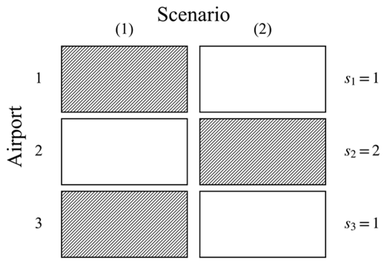
As an example, consider a MAS with three airports $k\in \{1,2,3\}$ and a shared fix $q$. The flow at fix $q$ is contributed by the arrival/departure flow from all three airports in the MAS. For each airport, there are two slot execution deviation scenarios $a_k\in \{1,2\}$, and their scenario combination is denoted as $(a_1,a_2,a_3)$. For the scenario combination (1,2,1), as shown in Figure 2, the flow fix $q$ within window $w$ is given by:

$$\sum _{n\in T_w}{({\beta }_{1,q,n+f_{1,q}^{arr}}^{arr(1)}+{\beta }_{1,q,n-f_{1,q}^{dep}}^{dep(1)}+{\beta }_{2,q,n+f_{2,q}^{arr}}^{arr(2)}+{\beta }_{2,q,n-f_{2,q}^{dep}}^{dep(2)}+{\beta }_{3,q,n+f_{3,q}^{arr}}^{arr(1)}+{\beta }_{3,q,n-f_{3,q}^{dep}}^{dep(1)})}^{\leftarrow }$$

The probability of occurrence for the scenario combination is:

$$P=p_1^{(1)}\cdot p_2^{(2)}\cdot p_3^{(1)}$$

Thus, the flow at fix $q$ within time window $w$ under different scenario combinations $g$ can be calculated, denoted as $Flo{w}_{q,w}^{(g)}$, as shown in Equation (28). The corresponding probability $P_{q,W}^{(g)}$ is represented as Equation (29):

$$Flo{w}_{q,w}^{(g)}=\sum _{n\in T_w}\sum _{k\in K}\left({\beta }_{k,q,n+f_{k,q}}^{arr(a_k)}+{\beta }_{k,q,n-f_{k,q}^{aep}}^{dep(a_k)}\right)$$

(28)

$$P_{q,w}^{(g)}=\prod _{k\in K}{p}_k^{arr(a_k)}/p_k^{dep(a_k)}$$

(29)

To transform the chance constraint, we introduce the 0–1 indicator variable ${\sigma }_{q,w}^{(g)}$ as shown in Equation (30), whose value is used to indicate whether the flow at fix $q$ within time window $w$ under scenario combination $g$ will satisfy the capacity constraint. When the flight flow $Flo{w}_{q,w}^{(g)}$ exceeds the fix capacity $C_q$, ${\sigma }_{q,w}^{(g)}=1$ is set; otherwise, ${\sigma }_{q,w}^{(g)}=0$ is set.

$${\sigma }_{q,w}^{(g)}=\left\{\begin{array}{c}1,Flo{w}_{q,w}^{(g)}>C_q\\ 0,Flo{w}_{q,w}^{(g)}\le C_q\end{array}\right.$$

(30)

To express this “conditional judgment” in a linear programming model, we introduce a sufficiently large positive number $M$. By using the Big-M method, we transform the nonlinear logic into a linear constraint; then, Equation (30) is equivalent to Equation (31):

$$Flo{w}_{q,w}^{(g)}\le C_q+M\cdot {\sigma }_{q,w}^{(g)}$$

(31)

where, when ${\sigma }_{q,w}^{(g)}=0$, the constraint simplifies to $Flo{w}_{q,w}^{(g)}\le C_q$, ensuring that the capacity is not exceeded; when ${\sigma }_{q,w}^{(g)}=1$, the constraint becomes $Flo{w}_{q,w}^{(g)}\le C_q+M$. Since $M$ is sufficiently large, this constraint imposes no actual restriction on the flow.

By utilizing the Big-M constraint, if the flow in a given scenario combination $g$ exceeds the capacity, it must hold that ${\sigma }_{q,w}^{(g)}=1$. In this way, we effectively “record” all scenario combinations that do not satisfy the capacity constraint. Since each scenario combination $g$ has an associated probability $P_{q,w}^{(g)}$, we can control the violation probability by taking the probability-weighted sum of all violation indicators across scenario combinations. To achieve this, we introduce the following aggregation constraint to ensure that the probability-weighted sum of violations for all scenario combinations at fix $q$ within time window $w$ does not exceed the allowed violation probability $\alpha$ under the chance constraint:

$$\sum _{g\in G}{P}_{q,w}^{(g)}\cdot {\sigma }_{q,w}^{(g)}\le \alpha$$

(32)

Thus, we have transformed the chance constraint into a deterministic constraint that reflects slot execution uncertainty. The CUSAM is represented by Equation (33) to Equation (38), with all constraints in the model being linear.

$$Z_a=min\left\{\sum _{n\in T}\sum _{i\in F^{arr}}\left|x_{i,n}^{arr}-O_{i,n}^{arr}\right|+\sum _{n\in T}\sum _{i\in F^{dep}}\left|x_{i,n}^{dep}-O_{i,n}^{dep}\right|\right\}$$

(33)

$$\sum _{g\in G}{P}_{q,w}^{(g)}\cdot {\sigma }_{q,w}^{(g)}\le \alpha ,\forall w\in D_w,\forall q\in Q$$

(34)

$$P_{q,w}^{(g)}=\prod _{k\in K}{p}_k^{arr(a_k)}/p_k^{dep(a_k)},\forall w\in D_w,\forall q\in Q$$

(35)

$$Flo{w}_{q,w}^{(g)}\le C_q+M\cdot {\sigma }_{q,w}^{(g)},\forall w\in D_w,\forall q\in Q$$

(36)

$$\sum _{n\in T_W}\sum _{k\in K}\left({\beta }_{k,q,n+f_{k,q}^{arr}}^{arr(a_k)}+{\beta }_{k,q,n-f_{k,q}^{aep}}^{dep(a_k)}\right)\le C_q,\forall w\in D_{\mathrm{w}},\forall q\in Q$$

(37)

$$Eq. (2) to Eq. (7),Eq. (10) to Eq. (11),Eq. (20) to Eq. (25)$$

(38)

2.4.2. Solution Technique for the CUSAM

In Section 2.4.1, we obtained the linear CUSAM that can be directly solved. We implemented the final solution using Python 3.9.7 and the Gurobi solver [41,42]. The model was run on a Windows 10 system with a 64-bit operating system, equipped with 16 GB of memory and an i7 processor.

2.5. The Scenario Generation Model (SGM)

To meet the solution requirements of the USAM, we establish a GMM-based slot execution deviation scenario generation model aimed at extracting typical scenarios and their occurrence probabilities. Below, we describe and formulate the SGM.

The input to the model consists of the historical slot execution deviation data of arrival/departure flights for a given airport within 24 hourly time windows across days, totaling 48 data sets. The output is the required number of slot execution deviation scenarios, where each scenario includes slot execution deviations of arrival/departure flights at the airport within the 24 hourly time windows across one day, totaling 48 values.

The model assumes that a data set $Z=\{z_1,z_2,\dots ,z_n\}$ consists of $A$ Gaussian distributions, where $A$ is the number of scenarios to be generated, and $z_i$ represents the preprocessed and standardized data points from the original data. Each Gaussian distribution has a clustering center ${\mu }_m$ (the mean in the GMM represents the center position of each Gaussian distribution in the standardized space, and these means are considered the clustering centers), variance ${\sigma }_m^2$, and mixing coefficient ${\pi }_m$, satisfying ${\displaystyle \sum _{m=1}^A}{\pi }_m=1$, where $m=1,2,\dots ,A$. The probability density function of the GMM is expressed as:

$$p(z_i)=\sum _{m=1}^A{\pi }_m\mathcal{N}(z_i| {\mu }_m,{\sigma }_m^2)$$

(39)

where $\mathcal{N}(z_i| {\mu }_m,{\sigma }_m^2)$ represents the probability density function of the $m$-th Gaussian distribution. Parameters $\{{\pi }_m,{\mu }_m,{\sigma }_m^2\}$ in the model are estimated using the Expectation–Maximization (EM) algorithm.

We define the 48 variables contained in the scenarios output by the SGM as $X_j(j=1,2,\dots ,48)$. These variables represent the slot execution deviations of arrival/departure flights within the 24 hourly time windows across one day. To generate a complete scenario, we combine the clustering results of the data sets to which these 48 variables belong. We perform independent GMM clustering for each variable $X_j$, obtaining the clustering centers ${\mu }_{j,{\mathfrak{m}}_j}$ and the mixing coefficients ${\pi }_{j,m_j}$ for each variable. We apply the inverse standardization transformation to convert the clustering centers into the original data scale, obtaining the inverse-standardized clustering centers ${\mu }_{j,m_j}^0$. The clustering centers used to form scenario $A_a$ are defined as ${\mu }_{j,m_j,a}^0$, and the mixing coefficients are defined as ${\pi }_{j,m_j,a}$. Thus, $A_a$ is represented by Equation (40):

$$A_a=\left\{{\mu }_{1,m_1,a}^0,{\mu }_{2,m_2,a}^0,\dots ,{\mu }_{48,m_{48},a}^0\right\}$$

(40)

The probability of the occurrence of scenario $A_a$, denoted as $P(A_a)$, is normalized and expressed by Equation (41):

$$P(A_a)={\displaystyle \frac{{\displaystyle \prod _{j=1}^{48}}{\pi }_{j,m_j,a}}{{\displaystyle \sum _{a=1}^A}{\displaystyle \prod _{j=1}^{48}}{\pi }_{j,m_j,a}}}$$

(41)

Thus, we have completed the construction of the SGM.

3. Case Study

We used real data provided by the North China Air Traffic Management Bureau to implement the proposed model. In Section 3.1, we describe the experimental setup, including the model’s inputs and outputs, as well as the selection of the research subjects. In Section 3.2, we present the optimization results of the model and analyze their robustness in Section 3.3.

3.1. Experiment Setup

We selected the MAS of Beijing–Tianjin in China as the research subject. The MAS spans two municipalities and includes airport ZBAA, ZBAD, and ZBTJ. As shown in Figure 1, the airspace of the MAS is complex, with multiple air routes intersecting, and several airports share the same fix. We used the flight schedule data of the MAS of Beijing–Tianjin for the winter–spring season of 2019. Given the low variability of daily flight schedules during a season, we chose the schedule data for October 28th as the model input. According to statistics, there were a total of 2381 scheduled flights in the MAS on 28 October 2019, including 1198 arrivals and 1183 departures.

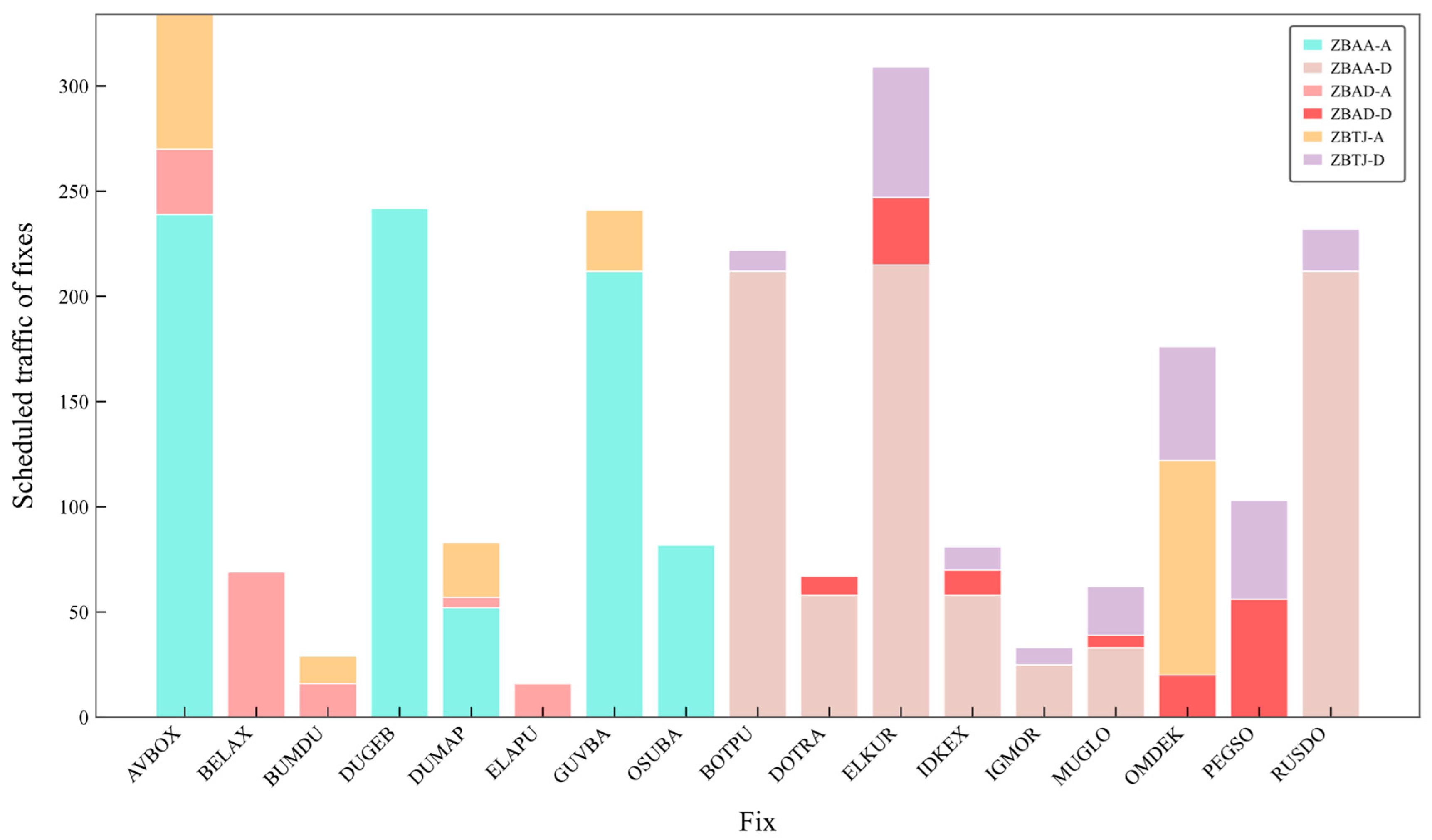
We selected the four fixes AVBOX, ELKUR, GUVBA, and RUSDO with high traffic shared by multiple airports, as shown in Figure 3, for the fix capacity constraints. In the legend of Figure 3, -A/-D represents the arrival/departure flights from airports. For example, ZBAA-A indicates the scheduled traffic of the departure flights from ZBAA at the fix. Additionally, in the USAM, we rewrote the capacity constraint for the fix AVBOX, which had the highest scheduled traffic share for the day and served as the shared arrival fix for all three airports, as a chance constraint (its geographic location is highlighted in blue in Figure 1), defining it as a “chance-constrained fix”.

In the scenario generation, we set the number of the slot execution deviation scenario for each airport $A=2$. The reasons for this choice are as follows:

1.

The purpose of this study is not to explore the impact of deviations in slot execution on optimization but rather to propose a method for addressing slot execution uncertainty. Therefore, we opted for a simpler scenario setup.

2.

The MAS in the experiment includes three airports. Even if only two slot execution deviation scenarios are generated for each airport, the total number of scenario combinations for the entire MAS would be 2³ = 8. Additionally, the generated slot execution deviation scenarios encompass deviations for all arrival and departure flights within 24 hourly time windows across a day, which significantly increases the overall complexity.

The flying time in the model was based on the median of historical flying times. Other input data sources have been provided in Section 2 and will not be reiterated here.

3.2. Results

3.2.1. Scenario Generation Results

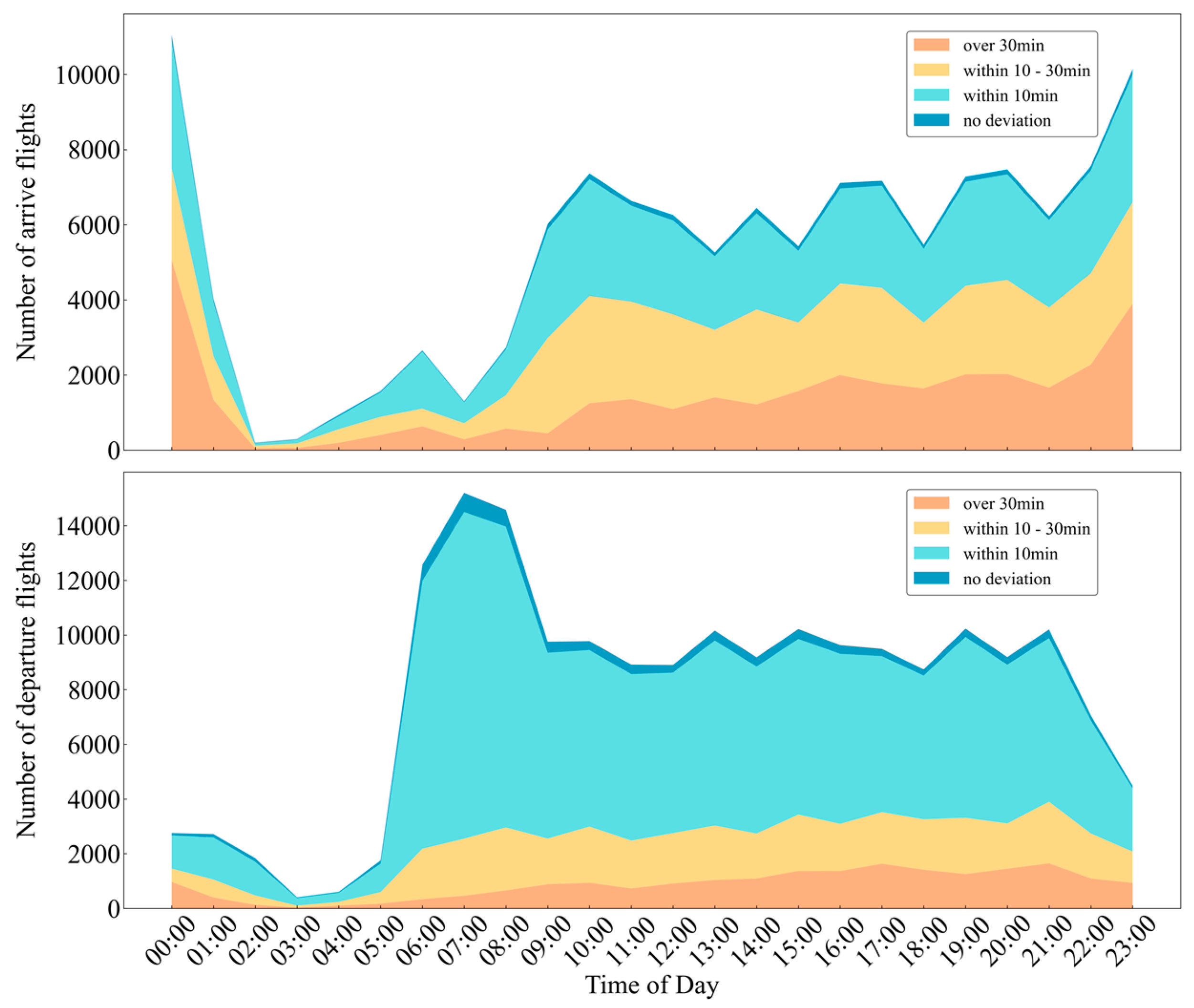
Figure 4 shows the slot execution deviation at airport ZBAA in 2019. The values on the vertical axis in Figure 4 represent the statistical numbers of different slot execution deviation situations for arrival/departure flights. It can be observed that flights that strictly adhered to their assigned slots with no deviations were rare (with an average share of 3%), and a significant portion of the flights had slot execution deviations within 10 min (with an average share of 52%). We applied the model from Section 2 to generate scenarios for the three airports in the MAS, setting $A=2$. To generate typical scenarios, we limited the slot execution deviations in the generated scenarios to no more than 10 min. The results are shown in

Table 2. Results of scenario generation.

Airport	Scenario	Probability	-A/-D	Slot Execution Deviation for Hour-Based Time Window of a Day (min)
				00:00	01:00	02:00	03:00	04:00	…	18:00	19:00	20:00	21:00	22:00	23:00
ZBAA	$A_1$	0.513	-A	−3	−5	4	3	3	…	5	−5	−5	−6	4	−5
			-D	2	−5	3	1	−1	…	−7	2	1	−6	1	−8
	$A_2$	0.487	-A	5	4	4	−1	2	…	5	−5	4	4	−5	4
			-D	−6	4	−6	−8	−3	…	2	−7	−7	3	−7	0
ZBAD	$A_1$	0.675	-A	5	4	4	−6	−7	…	3	−5	4	4	−5	4
			-D	−1	−2	−1	4	7	…	7	7	0	0	6	7
	$A_2$	0.325	-A	3	−6	−7	−5	5	…	2	3	4	−6	3	3
			-D	6	7	6	−5	1	…	0	0	7	7	−1	−1
ZBTJ	$A_1$	0.792	-A	4	6	−3	−5	−2	…	−1	3	−1	−4	−5	−8
			-D	−1	−2	−1	4	7	…	7	7	0	0	6	7
	$A_2$	0.208	-A	−6	3	4	7	4	…	2	4	3	−3	−6	−6
			-D	6	7	6	−5	1	…	0	0	7	7	−1	−1

.

This paper set three schemes to compare the optimization results, as shown in

Table 3. Optimization schemes.

Schemes	Experimental Objects
Schemes 0	None
Schemes 1	All
Schemes 2(a)	ZBAA
Schemes 2(b)	ZBTJ
Schemes 2(c)	ZBAD

. Scheme 0 did not consider slot execution deviation and used the CSAM for solving, serving as a control group for the USAM. Scheme 1 considered the slot execution deviation for all three airports within the MAS, while Scheme 2 separately considered the slot execution deviation for each of three airports, both using the USAM for solving. For the chance-constrained fix, various violation probabilities were set to explore optimization solutions under varying levels of acceptability.

3.2.2. Optimization Results

The total displacements presented in 5 min intervals corresponding to different violation probabilities in the schemes are shown in

Table 4. Displacements in the schemes.

Schemes	Experimental Objects	Adjustments (5 min)
		$\mathit{\alpha }=0$	$\mathit{\alpha }=0.1$	$\mathit{\alpha }=0.2$	$\mathit{\alpha }=0.3$	$\mathit{\alpha }=0.4$
Schemes 0	None	192	192	192	192	192
Schemes 1	All	362	358	324	279	237
Schemes 2(a)	ZBAA	298	298	298	298	298
Schemes 2(b)	ZBTJ	215	215	215	193	193
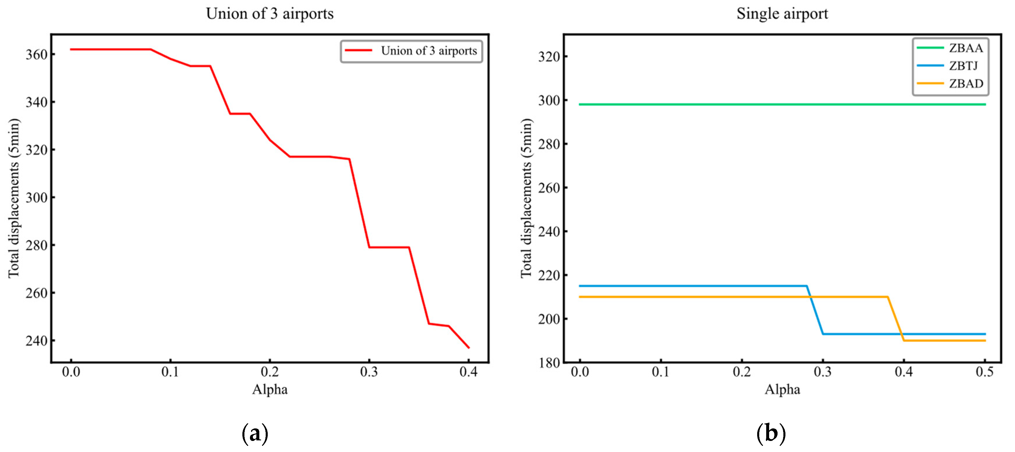
Schemes 2(c)	ZBAD	210	210	210	210	190

. For all schemes, the total displacement increased as the violation probability decreased. This was clearly because a smaller violation probability makes the constraint more stringent, resulting in a more conservative model.

It can be observed in Figure 5a that the total displacement decreased sharply in a step-like manner as $\alpha$ increased in Scheme 1. There were also intervals where the total displacement remained constant, such as $\alpha \in [0.22,0.28]$. The optimization results of Scheme 2, as shown in Figure 5b, further confirm this discontinuous response characteristic, with more noticeable phase transition features. In the optimization results of Scheme 2(b) and Scheme 2(c), there was a sudden change in the total displacement at $\alpha =0.3$ and $\alpha =0.4$, respectively. For Scheme 2(a), the total displacement remained constant throughout the entire selected range of $\alpha$. Upon analysis, the primary reason for the observed characteristics was as follows: To solve the USAM, we propose the CUSAM, which converts the violation probability constraint in the chance constraint into a constraint for the total probability of scenario combinations violating the capacity constraint, based on the discrete distribution of random variables. The occurrence probability of a scenario combination is composed of several discrete scenarios (for example, in Scheme 1, there are eight scenario combinations, with each combination’s probability derived from the discrete probabilities of the single airport’s scenarios). This joint probability distribution forms a discrete step function. The intervals with constant total displacements are due to this discreteness, where, within special intervals, the influence of scenario combinations on capacity constraints does not cause significant changes.

These characteristics indicate that when using the USAM, there are significant marginal benefit points, which can serve as key decision points for risk–cost trade-offs. There are also acceptable ranges, where further increasing the risk tolerance does not lead to significant gains as the optimization potential of the original schedule has already been fully explored.

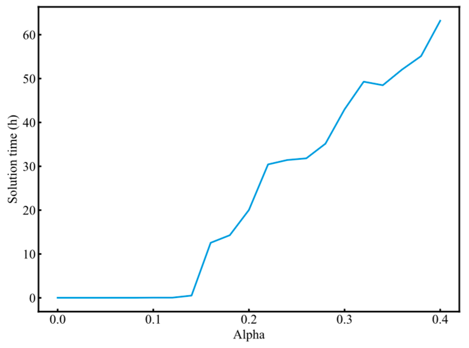
During the model solving process, we observed that the convergence time of the model significantly increased as the violation probability rose. By averaging the solving times for multiple runs with the same violation probability in Scheme 1 (as shown in Figure 6), we found that when $\alpha$ increased from 0.1 to 0.4, the average solving time rose from 0.02 h to 63.18 h, a 2675% increase. We attribute this to the intrinsic difficulty of optimization with chance constraints under a discrete probability distribution; when constructing the CUSAM framework, the distribution function of fix traffic is constrained by the discrete nature of scenario combinations, preventing a unified analytical form. To address this, we introduce auxiliary variables ${\sigma }_{q,w}^{(g)}$ to equivalently transform the chance constraints. The values of each ${\sigma }_{q,w}^{(g)}$ propagate to adjacent decision variables, resulting in a cascade of feasible solution derivations. While increasing $\alpha$ relaxes the constraint boundaries, it leads to a non-convex fractal expansion of the feasible solution space, causing the algorithm to face an explosion of combinations during the search, greatly increasing convergence difficulty. This indicates that within a discrete probability framework, balancing robustness and optimality requires super-linear computational costs. It also implies that while the model can easily provide a highly conservative solution, pursuing an optimal compromise by sacrificing some robustness is relatively more challenging.

3.3. Robustness of the Results

The aim of considering slot execution uncertainty is to enhance the robustness of the strategic schedule, ensuring capacity–flow balance across various scenarios. In this section, we validate the practical effectiveness of the model by comparing the flow performance at the chance-constrained fix under different optimization schemes.

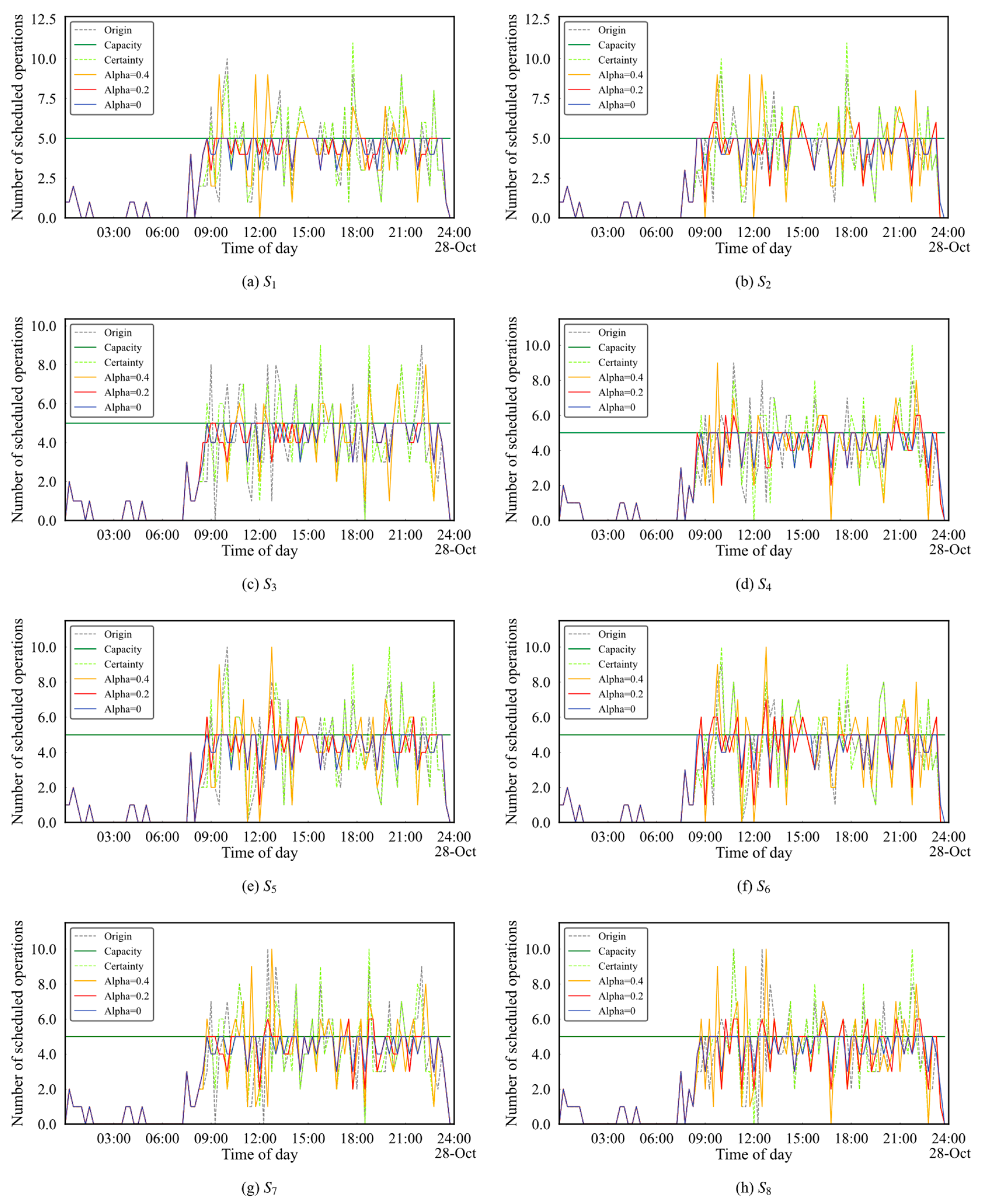
Firstly, to investigate the performance of the USAM results under different scenario combinations, we selected the optimization results of Scheme 1 and calculated the scheduled traffic for each 15 min time window under all eight scenario combinations ($S_1$ to $S_8$), as shown in Figure 7, where “Origin” represents the original schedule, “Capacity” denotes the 15 min capacity of the fix, “Certainty” indicates the CSAM results, and “Alpha = 0, Alpha = 0.2, Alpha = 0.4” represent the USAM results under different violation probabilities, respectively.

From Figure 7, it can be observed that the results of CSAM failed to demonstrate positive effects and even exhibited negative impacts in most scenario combinations. For instance, in scenario combinations $S_3$, $S_4$, $S_5$, and $S_7$, the performance of peak flow became more severe compared to the original schedule, manifested by an increase in the number of time windows with peak flow and a rise in excess flow (values of flow exceeding capacity). This indicates that neglecting slot execution uncertainty not only prevents achieving the desired optimization effects but may also exacerbate capacity–flow imbalance, ultimately leading to more flight delays.

In the USAM results, when Alpha = 0, the results satisfied the capacity requirements for all scenario combinations. When Alpha = 0.2, they satisfied requirements for $S_1$ and $S_3$. In other combinations, although there were a few time windows in which the flow slightly exceeded the capacity, the excess flow was relatively small. When Alpha = 0.4, the results showed significant improvement in terms of excess flow across all scenario combinations compared to the original schedule and the CASM results.

To some extent, the amount of excess flow reflects the robustness of the optimization results. The smaller the excess flow, the stronger the robustness. From this perspective, it is evident that the USAM significantly outperformed the CSAM in terms of robustness. Notably, in the original schedule, AVBOX exhibited four peak flow time windows (09:00–10:00, 12:00–13:00, 18:00–19:00, and 22:00–23:00) in most scenario combinations. In the USAM results, these peak periods were smoothed to varying degrees, meaning that some flights originally scheduled during peak hours were adjusted to other time windows. A smoother flow distribution implies fewer delays. When Alpha = 0, the flow distribution was the smoothest; however, this came at the cost of the largest adjustment. When Alpha = 0.2 and Alpha = 0.4, the peak flows were partially smoothed, but this is more realistic than a completely flat flow distribution while still accommodating potential flow demands.

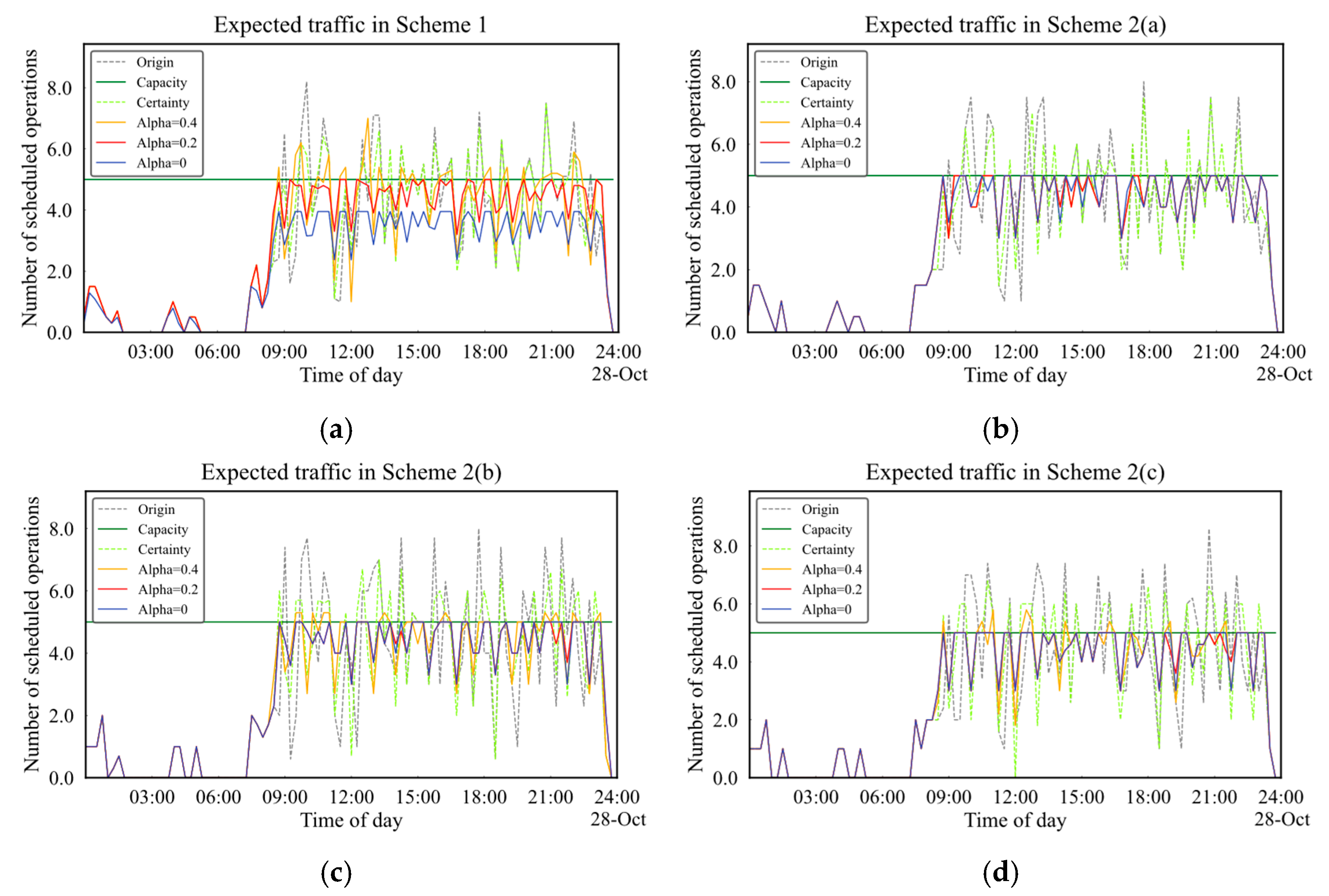
The expected flow reflects a compromise scenario, representing the average flow scale under various scenario combinations. From Figure 8, it can be observed that both the original schedule and the CSAM results exhibited severe capacity exceedance in all schemes. This was clearly because the CSAM does not account for slot execution uncertainty. In contrast, the USAM results, whether considering slot execution deviation for the MAS or individual airports, satisfied the capacity constraints for all time windows when Alpha = 0 and Alpha = 0.2. Even when Alpha = 0.4, the excess flow was significantly improved in the few time windows where the capacity was exceeded. For example, in Scheme 1, for the MAS, compared with the results of the CSAM and the original schedule, the number of peak time flow windows (where the flow value exceeds 6) decreased by 84.6% and 75% respectively. For the result of Scheme 1, when Alpha = 0, the expected flow remained consistently below 4, which, given the capacity limit of 5, not only satisfies the capacity constraints but also reserves room for tactical adjustments.

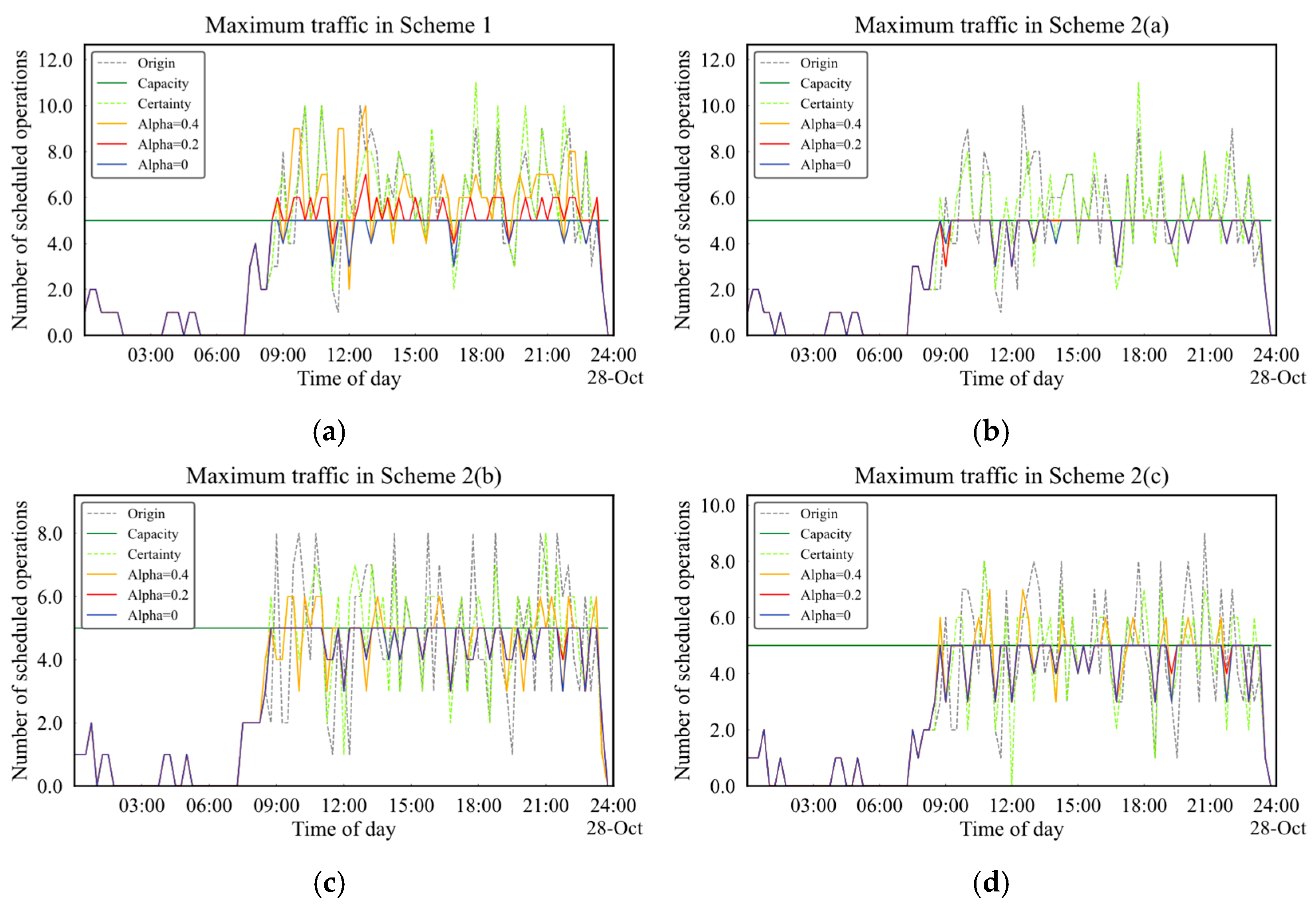
The maximum flow reflects a worst-case scenario, representing the highest flow achievable in each time window under various scenario combinations. As shown in Figure 9, compared to the scheduled flow and expected flow, the original schedule and CSAM results exhibited a significant increase in the number of time windows with capacity exceedance and a higher excess flow under the maximum flow scenario. In contrast, the USAM results satisfied the capacity constraint for all schemes when Alpha = 0, making the model fully robust. When the violation probability increased to Alpha = 0.2, the capacity constraints for all single-airport schemes were still met. Although capacity exceedance occurred when Alpha = 0.4, both the number of exceedance time windows and the excess flow were significantly improved. For example, in Scheme 1, for the MAS, compared with the results of the CSAM and the original schedule, the average maximum values of traffic flow in the maximum traffic flow statistics decreased by 31.1% and 33.5%, respectively. It is worth noting that we observed that the solutions of the USAM were not unique. For example, in Scheme 2(c), the total displacement was the same for Alpha = 0 and Alpha = 0.2 (Table 1), and as shown in Figure 9, the results for both violation probabilities satisfied the capacity constraints for all time windows, but the maximum flow differed in specific time windows (19:30–19:45 and 22:00–22:15). This implies that when using the USAM, slot coordinators can select the most suitable scheme based on preferences, such as airline operating costs or passenger travel time preferences.

In this section, we demonstrate across three dimensions—scheduled flow performance under scenario combinations, expected flow performance, and maximum flow performance—that the optimization results of the proposed USAM exhibit significantly greater robustness compared to those of the CASM.

4. Conclusions

This paper focuses on slot allocation for the MAS and begins by formulating a CSAM. Formulating upon the CSAM, we develop a USAM considering slot execution uncertainty, aiming to enhance the robustness of the strategic schedule under slot execution deviation scenarios and to effectively utilize airport and airspace capacities. In the USAM, we rewrite the capacity constraint of fixes as the chance constraint. We employ a method to transform the chance constraint into the deterministic constraint, relying on the discrete distribution law of the fix flow. This transformation results in the CUSAM, an MIPM that can be directly applied to solvers. Additionally, we develop a SGM to derive slot execution deviation scenarios and their probability distributions for different airports, the results of which are utilized in solving USAM. Finally, we implement the model using the Gurobi solver.

We applied the USAM to the MAS of Beijing–Tianjin in China and obtained optimized strategic schedules under different schemes. We analyzed the variation patterns of the total slot displacement and solution time with respect to violation probabilities. Furthermore, we evaluated the robustness of the results from the USAM using three metrics: scheduled flow performance under different scenario combinations, expected flow performance, and maximum flow performance. The results show that compared to the optimization results of the CSAM and the original schedule, the USAM significantly enhanced the robustness of the strategic schedule at the cost of the relatively larger total slot displacement.

The main contributions of this paper are as follows:

• A certainty slot allocation model is proposed, which takes comprehensive capacity constraints into account.
• Based on the certainty model, a chance-constrained slot allocation model considering slot execution uncertainty is proposed. Experimental results show that the model significantly improves the robustness of strategic schedules. Moreover, the introduction of the chance constraint achieves a balance between robustness and optimality, providing slot coordinators with flexible optimization solutions based on their acceptable levels of risk while offering references for tactical-level flow management plans.
• A transformation method for the chance constraint based on stochastic programming theory is proposed, which converts the complex and hard-to-solve uncertainty model into a tractable certainty linear model for efficient solving.
• A scenario generation method for slot execution uncertainty is proposed. It captures typical scenarios and their occurrence probabilities from historical data to support the solution of the model described above.

However, this study has some limitations that warrant further exploration. The inherent limitations of the proposed method are summarized as follows:

• The proposed SGM is based on the assumption of statistical independence of slot execution deviations, which fails to fully capture spatiotemporal coupling effects in actual operations, such as airspace congestion interactions and delay propagation in airport networks.
• The traditional solver used in this study shows limited efficiency when dealing with high-dimensional and complex scenario combinations, making it difficult to support the efficient solution of the large-scale chance-constrained model.
• Our model captures the outcome-level uncertainty, and we did not sufficiently elaborate on the role of human factors in shaping such uncertainties.

In future work, we aim to improve the SGM to better reflect real-world operational characteristics. Specifically, we will explore data-driven deep learning methods to construct a spatiotemporal attention mechanism based on graph neural networks. Airports are treated as graph nodes, while dynamic edge weights, such as flow and meteorological conditions, are used to characterize the influence intensity, thereby supplementing and refining the SGM. Traditional MIP solvers’ preset heuristic strategies are significantly limited in such high-dimensional, irregular solution spaces, and solving difficulty will increase substantially as scenario combinations become more complex. To address this, we may need to develop new algorithms to tackle these computational challenges. Specifically, we will explore a collaborative framework that integrates intelligent heuristics with exact solution methods. We plan to design metaheuristic algorithms tailored to the problem’s characteristics, such as enhanced genetic algorithms and tabu search, to generate high-quality initial solutions. These solutions will help identify promising regions of the solution space through a pre-screening mechanism. The feasible solutions obtained from the heuristics will then serve as warm-start inputs for the MIPM, ensuring solution accuracy while improving convergence efficiency. Additionally, we will investigate classical algorithms for MIPM, such as Bender’s decomposition, which decomposes the problem into a master problem and subproblems. To address the aforementioned issue of scenario combination explosion, we will develop acceleration schemes based on scenario clustering, aiming to tackle the computational challenges effectively. In addition, we aim to explore behavioral modeling and data-driven approaches, such as learning decision patterns from historical data, to capture the dynamics of human-in-the-loop systems more effectively for considering the role of human factors. We believe this is a promising direction that will significantly improve the practical value of our research. Going forward, the proposed slot execution uncertainty-aware modeling and the chance constraint transformation method can also be applied to other problems in civil aviation. For instance, in air traffic flow management (ATFM), the uncertainty can affect flow prediction and scheduling across the entire airspace, potentially becoming core challenges in flight sequencing and dynamic sector capacity adjustments. Additionally, the USAM essentially solves a stochastic constrained resource allocation problem, and its modeling approach can be universally applied to all such resource-constrained production scheduling optimization problems.