Manifold Learning for Aerodynamic Shape Design Optimization

Abstract

The significant computational cost incurred due to the iterative nature of Computational Fluid Dynamics (CFD) in traditional aerodynamic shape design frameworks poses a major challenge, especially in the context of modern integrated design requirements and increasingly complex design conditions. To address the demands of modern design, we developed an efficient aerodynamic shape design framework based on our previous work involving the locally linear embedding plus constrained optimization genetic algorithm (LLE+COGA) high-fidelity reduced-order model (ROM). An active manifold (AM) auto-en/decoder was employed to address the dimensionality curse arising from an excessively large design space. The fast mesh deformation method was utilized for high-precision, rapid mesh deformation, significantly reducing the computational cost associated with transferring geometric deformations to CFD fine mesh. This work addressed the transonic optimization problem of the undeflected Common Research Model (uCRM) three-dimensional wing (with an aspect ratio of 9), involving 241 design variables. The results demonstrate that the optimized design achieved a significant reduction in the drag coefficient by 38.9% and 54.5% compared to the baseline in Case 1 and Case 2, respectively. Additionally, the total optimization time was shortened by 62.6% and 57.7% in the two cases. Moreover, the optimization outcomes aligned well with those obtained from the FOM-based framework, further validating the effectiveness and practical applicability of the proposed approach.

1. Introduction

Aerodynamic shape design plays a critical role in the aerospace industry, with profound impacts on the performance, fuel efficiency, and environmental sustainability of aircraft. For example, lift augmentation and drag reduction not only directly affect energy consumption and operational costs but also influence system stability, speed, and safety. Therefore, optimizing aerodynamic shapes to improve engineering efficiency and reduce carbon emissions, while ensuring safety and reliability, has become a key area of research. Traditional aerodynamic shape optimization problems are associated with linear and nonlinear partial differential equation (PDE)-based behavior functions. Solving such problems requires repeated evaluations of objective functions and constraints, such as through the nested analysis and design (NAND) approach [1,2]. While Computational Fluid Dynamics (CFD) methods provide accurate aerodynamic performance predictions, their computational cost and time consumption are substantial, particularly in high-fidelity simulations and complex flow conditions, which limit the efficiency of optimization and the feasibility of practical applications.

In this context, reduced-order models (ROMs) have become an effective tool to address this issue. ROMs simplify complex high-dimensional problems by retaining the main physical features of the system while eliminating less important degrees of freedom, thereby significantly reducing computational complexity and cost. Many techniques have been proposed for model order reduction in high-dimensional models (HDMs), such as manifold learning, the Volterra series, proper orthogonal decomposition (POD), and dynamic mode decomposition (DMD) [3,4,5,6]. Additionally, within the broader context of intelligent fluids, a series of reduced-order models based on intelligent algorithms have emerged [7,8,9,10,11]. It is important to note that different reduced-order models (ROMs) are suitable for different application scenarios. For rapid aerodynamic shape optimization design, ROMs must meet two key requirements. On one hand, the sampling space should be as small as possible to avoid excessive cost associated with constructing the sampling space (often obtained through full-order model (FOM) simulations or wind tunnel experiments). On the other hand, the model should provide high prediction accuracy. The LLE+COGA replaces traditional interpolation with a high-precision, low-dimensional prediction approach based on manifold learning geometric constraints combined with genetic algorithms (GAs). This method compensates for the inherent information loss in the dimensionality reduction process and effectively utilizes the geometric information of the high-dimensional space, requiring a smaller sampling space for the same prediction accuracy. Reference [12] demonstrates, through examples of transonic strong nonlinear aerodynamic load prediction for both 2D airfoils and 3D wing–body configurations, that this reduced-order model achieves high prediction accuracy. Therefore, the LLE+COGA high-fidelity reduced-order model effectively meets the aforementioned requirements and can be used to accelerate aerodynamic shape optimization design.

Aerodynamic shape optimization design is a major application area of ROMs [13,14,15,16,17,18,19,20,21]. The main challenge faced by aerodynamic shape optimization frameworks is the “curse of dimensionality” caused by an excessively large design space. Currently, two primary solutions are available: the adjoint method and design space dimensionality reduction. The adjoint method is widely used in aerodynamic shape optimization design. It calculates the sensitivity of design variables to the objective function (e.g., drag, lift) by solving the adjoint equations, thus enabling effective gradient-based optimization. While the adjoint method can handle high-dimensional design variable spaces, it requires solving the adjoint equations and calculating the gradients of the objective and constraints with respect to the design variables which can incur high computational costs. This is particularly challenging when dealing with nonlinearities, complex boundary conditions, or turbulence, as the solution of the adjoint equations becomes more difficult, potentially leading to model instability or poor convergence. Furthermore, the form of the adjoint equations and the solution method may vary under different optimization objectives and constraint conditions, adding to the complexity of implementation. Additionally, the method faces challenges in handling irregular, complex geometries, relies on high-quality meshes, and is sensitive to initial conditions. To avoid the computational resource consumption associated with gradient calculation, and to address issues such as gradient vanishing that can arise with certain reduced-order algorithms, design space dimensionality reduction has been widely researched. Boncoraglio and Farhat [1] proposed the active manifold (AM) method, which assumes that the solution to the optimization problem depends on a low-dimensional nonlinear manifold. Their research found that AM outperforms active subspace (AS) techniques, such as the basic AS method [22] and enhanced AS method [23], in terms of performance. In addition, the acceleration of data transfer between geometric parameterization deformation and CFD mesh deformation is often overlooked. However, with the increasing complexity of geometric shapes and the widespread use of unstructured meshes, this issue has become more prominent. Taking the Radial Basis Function (RBF) dynamic mesh technique as an example, CFD meshes near the geometric surface often exhibit a large number of locally refined points. If all mesh points are selected, the resulting matrix computations incur substantial computational costs. Moreover, the excessive density of local data points may lead to numerical instability in the matrix operations, potentially resulting in errors. This work improves the efficiency of mesh deformation through the fast mesh deformation method based on a greedy algorithm.

This study aims to validate the feasibility of the high-fidelity nonlinear reduced-order model (LLE+COGA) in addressing aerodynamic optimization problems and to establish a novel rapid aerodynamic shape optimization framework. The proposed framework seeks to mitigate the excessive computational resource consumption associated with full-order optimization, thereby enhancing optimization efficiency. Furthermore, this research introduces a fast mesh deformation algorithm, which reduces the number of surface deformation control points to eliminate unnecessary computational resource expenditure. The remainder of this paper is organized as follows. Section 2 formulates a general aerodynamic optimization design problem to ensure that this article is as self-contained as possible. Section 3 describes the proposed optimization design framework. Section 4 validates the proposed rapid aerodynamic optimization design framework by solving the transonic optimization problem of the undeflected Common Research Model (uCRM) three-dimensional wing (with a span-to-chord ratio of 9), which involves 241 design variables. Section 5 provides a detailed analysis of the optimization results.

2. Problem Formulation

This study focuses on accelerating the aerodynamic shape optimization design problem, which includes both equality and inequality constraints. Such problems can be expressed in the following general form, as shown in Equation (1):

$$\begin{array}{cc}\underset{q,\mu }{min}\hfill & f(q,\mu )\hfill \\ \mathrm{subject}\mathrm{to}\hfill & c(q,\mu )\le 0\hfill \\ \hfill & R(q,\mu )=0\hfill \end{array}$$

(1)

where $f(·)$ represents a scalar objective function to minimize and $q\in {\mathbb{R}}^{N_q}$ denotes a high-dimensional vector of $N_q$ semidiscrete or discrete state variables involved in a high-dimensional, parametric, linear or nonlinear constraint. $\mu \in \mathcal{D}\subset {\mathbb{R}}^{N_D}$ denotes a vector of the dimensions $N_{\mu }$ of design optimization parameters that typically represents displacement deformation in the context of aerodynamic shape optimization problems. $\mathcal{D}$ represents the high-dimensional design space, where it is assumed that $N_{\mu }=N_{\mathcal{D}}$ is relatively large (say, $N_{\mu }\ge 50$) [1]. $c(·)$ represents a collection of both linear and nonlinear algebraic constraints. $R(q,\mu )$ is a parametric PDE in q that is either semidiscretized or fully discretized in a high-dimensional space.

In practical problems, only the design variable $\mu$ needs to be optimized. Therefore, in the nested analysis and design (NAND) approach, the state variable q can be treated as an implicit function of $\mu$. By solving the PDE constraint R, Equation (1) can be rewritten as Equation (2):

$$\begin{array}{cc}\hfill \underset{q,\mu }{min}& f(q,\mu )\hfill \\ \hfill \mathrm{subject}\mathrm{to}& c(q,\mu )\le 0\hfill \\ \hfill & R(q,\mu )=0\hfill \end{array}\Rightarrow \begin{array}{cc}\hfill \underset{\mu \in \mathcal{D}}{min}& f\left(q\right(\mu ),\mu )\hfill \\ \hfill \mathrm{subject}\mathrm{to}& c\left(q\right(\mu ),\mu )\le 0\hfill \end{array}$$

(2)

The design variable in the i-th iteration is denoted as ${\mu }_i\in \mathcal{D}$, and $q\left({\mu }_i\right)$ is obtained by solving $R(q,\mu )=0$. This process can be written as Equation (3).

$${\mu }_i\to R(q\left({\mu }_i\right),{\mu }_i)=0\to q=q\left({\mu }_i\right)$$

(3)

It is important to note that as the dimension of the design space $\mathcal{D}$ increases, the computational cost of evaluating the objective function $f(·)$ and algebraic constraints $c(·)$ increases rapidly. Therefore, the development of new, efficient optimization frameworks is of significant importance.

3. Innovative Optimization Framework

The fast aerodynamic shape optimization design framework based on ROMs is shown in Figure 1. If a flow solver is used to compute the flow state variables and an adjoint solver is used to compute the gradients, this corresponds to the traditional adjoint-based optimization design framework, represented by the grey portion in the figure.

The solution of the flow control equations and the adjoint equations accounts for the majority of the computational cost in the traditional adjoint-based optimization framework. By replacing the FOMs with ROMs, not only can simulation time be significantly reduced, but solving the adjoint equations can also be avoided. It is worth noting that the computational cost associated with updating the CFD mesh due to geometric deformations is increasingly difficult to ignore. This is because complex geometric models often involve regions of local refinement near the surface, which leads to substantial matrix computation resource consumption for the mesh deformation algorithms. Furthermore, there is a risk that the dense distribution of mesh data points could cause numerical instability or even numerical errors, ultimately resulting in non-physical solutions in the optimization process. In addition, it is necessary to avoid the issue of the “curse of dimensionality” caused by excessively high dimensions in the design space.

3.1. Geometric Parameterization

The Free-Form Deformation (FFD) geometry parameterization method used in this study is a shape modeling technique employed in computer graphics and computer-aided design (CAD), widely applied for geometric deformation modeling [24]. The FFD volume is used to parameterize changes in geometry rather than the geometry itself, leading to a more compact and efficient representation of design variables, which simplifies the manipulation of complex shapes. Any geometry can be embedded within the volume by applying a Newton search to map the parameter space to the physical space. Geometric modifications are applied to the outer boundary of the FFD volume, and any adjustments to this boundary indirectly affect the embedded geometries. A key assumption of the FFD method is that the geometry maintains constant topology throughout the optimization process, which is typically true in wing design. Additionally, because FFD volumes are based on trivariate B-splines, the derivatives of any point within the volume can be easily computed [25,26].

3.2. Reduced-Order Model: LLE+COGA

It is aspirational to construct a nonlinear reduced-order model (ROM) with the ability to predict Computational Fluid Dynamics (CFD) solutions accurately and efficiently. In our previous work, we proposed a novel, high-fidelity, nonlinear reduced-order model: the locally linear embedding plus constrained optimization genetic algorithm (LLE+COGA) [12]. Our research found that one major challenge is that the nonlinearity cannot be adequately captured by interpolation algorithms in low-dimensional space. This implies that an ROM based on a dimensionality reduction algorithm combined with traditional interpolation methods requires a larger sampling space to achieve the same low-dimensional prediction accuracy as the COGA, without incorporating additional low-dimensional predictive information. This, in turn, leads to a higher computational resource consumption. To preserve the nonlinearity of CFD solutions for transonic flows, a new ROM is presented by integrating manifold learning (ML) into constrained optimization, whereby a neighborhood preserving mapping is constructed by a locally linear embedding (LLE) algorithm. Reconstruction errors are minimized by LLE by solving a least-square problem subject to weight constraints. The low-dimensional space obtained through LLE dimensionality reduction preserves the same geometric features as the high-dimensional space under the algorithm’s assumptions and can be expressed as Equation (4):

$$X_i={\Omega }_i^T{X}_{N_i}\to x_i={\Omega }_i^T{x}_{N_i}$$

(4)

where $X_i$ represents the i-th point in the high-dimensional space, and $x_i$ denotes its corresponding point in the low-dimensional manifold space. $X_{N_i}$ and $x_{N_i}$ correspond to the neighboring points in the high-dimensional and low-dimensional spaces, respectively. The low-dimensional manifold preserves the same neighborhood relationships as the high-dimensional space, denoted as ${\Omega }_i$. A loss function is proposed in the constrained optimization to preserve the geometric properties between high-dimensional space and low-dimensional manifolds, as shown in Equation (5).

$$\mathcal{F}=min\parallel D_{G{A}_i}-d_{G{A}_i}{\parallel }_2.$$

(5)

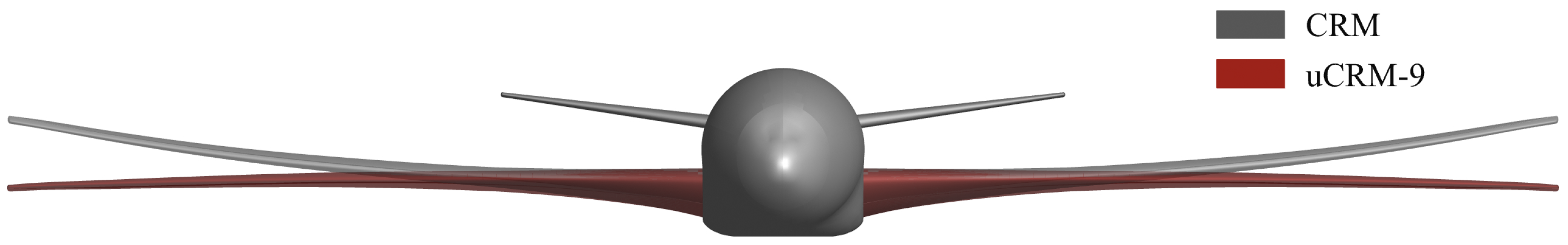
$d_{G{A}_i}$ represents the Euclidean distance vector between the i-th iteration’s low-dimensional predicted results and its neighboring points, while $D_{G{A}_i}$ denotes the corresponding high-dimensional Euclidean distance vector under the same neighborhood relationship coefficient. In our previous research, the LLE+COGA was validated for predicting nonlinear transonic flows over the RAE 2822 airfoil and the undeflected NASA Common Research Model with an aspect ratio of 9 (uCRM-9), where nonlinearities were induced by shock waves. All results confirmed that the reduced-order model (ROM) accurately replicated CFD solutions at a fraction of the cost compared to CFD calculations or full-order modeling (FOM). For specific details, please refer to reference [12].

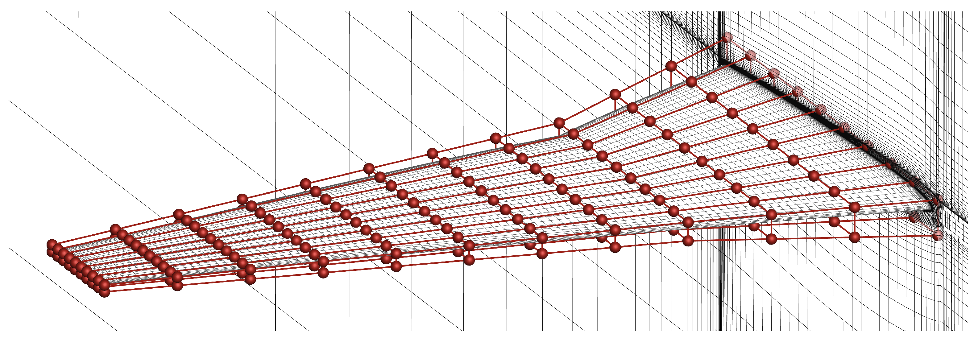
3.3. Fast Mesh Deformation

For CFD surface meshes with significant local refinement, it is necessary to quickly propagate the deformation to the CFD volume mesh in order to minimize computational costs. Taking the Radial Basis Function (RBF) mesh deformation algorithm as an example, it can be represented in the following form, as shown in Equation (6):

$$\begin{array}{c}\hfill \left\{\begin{array}{c}∆d_{surf}=M_{ss}\alpha \hfill \\ ∆d_{vol}=M_{vs}\alpha \hfill \end{array}\right.\end{array}$$

(6)

Here, $∆d$ represents the displacement, and $\alpha$ denotes the Radial Basis Function (RBF) interpolation coefficient. The subscripts s and v refer to the surface mesh quantities and volume mesh quantities, respectively. The matrix $M_{vs}$ is represented as Equation (7), and $M_{ss}$ is similarly represented.

$$\begin{array}{c}\hfill M_{vs}=\left[\begin{array}{ccc}\varphi (p_{v1},p_{s1})& \cdots & \varphi (p_{v1},p_{ss})\\ ⋮& \ddots & ⋮\\ \varphi (p_{vv},p_{s1})& \cdots & \varphi (p_{vv},p_{ss})\end{array}\right]\end{array}\begin{array}{cc}\hfill & {\xi }_{ij}={\displaystyle \frac{\parallel p_i-p_j\parallel }{R_{RBF}}}\left\{\begin{array}{cc}{\xi }_{ij}=1\hfill & if{\xi }_{ij}\ge 1\hfill \\ {\xi }_{ij}={\xi }_{ij}\hfill & else\hfill \end{array}\right.\hfill \\ \hfill & \varphi \left(\xi \right)={(1-\xi )}^4\times (4\xi +1)\hfill \end{array}$$

(7)

From Equation (7), it can be observed that if there are too many surface points, the dimension of the matrix M will increase, thereby raising the computational cost of solving the Radial Basis Function (RBF) deformation coefficients. Additionally, if there are too many points with very small Euclidean distances, it could lead to matrix singularity, causing numerical instability or even errors in the solution. Therefore, it is necessary to minimize the number of surface control points involved in the mesh deformation while ensuring the accuracy of the results. A greedy algorithm is employed here to select surface control points, as shown in Algorithm 1. The specific process is as follows:

• Deform the geometry in the design variable space;
• Select the two points that are the farthest apart in terms of Euclidean distance within the point set as the initial values for the iteration;
• Use the selected points as surface control points, compute the RBF deformation results, and calculate the error between the deformed points and the original point set. Add the point with the largest error to the selected set, and repeat the process until the predefined acceptable error limit is reached.

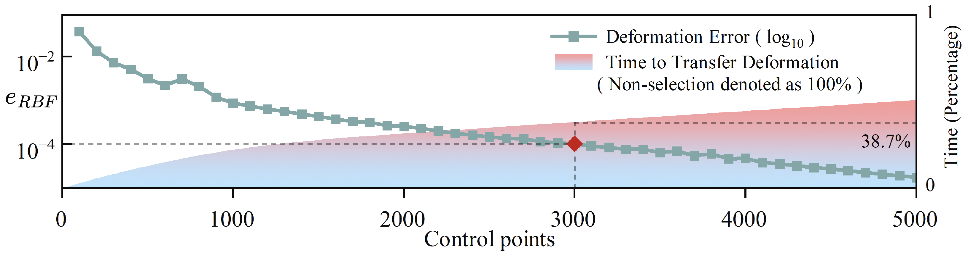
In other words, under limited computational resources, by restricting the number of surface control points to the same amount, the fast mesh deformation method can minimize the error.

Algorithm 1 Greedy selection of deformation points.

Input: All Surface Mesh Points: $P=[P_1;P_2;\cdots ;P_N]$ Output: Selected Points for Deformation: $P_s=[{\overline{P}}_1;{\overline{P}}_2;\cdots ;{\overline{P}}_s]$ 1: $P_{\mathrm{deformation}}\leftarrow FFD(\mu ,P)$   ▹ Manually deform mesh based on surface sensitivity 2: $P_s^{i=2}=\{{\overline{P}}_1;{\overline{P}}_2\}$    ▹ A randomly selected point and the point farthest from it in Euclidean distance form the initial set 3: for $i\leftarrow 3$ to s do            ▹ Start greedy point selection 4:     $P_{\mathrm{deformation}}^i\leftarrow RBF(P_s^{i-1},P)$        ▹ Reconstruct all points using $P_s^{i-1}$ 5:     ${\overline{P}}_i\leftarrow {\mathrm{error}}_{\max }(P_{\mathrm{deformation}}^i,P_{\mathrm{deformation}})$ 6:     $P_s^i=\{{\overline{P}}_1;{\overline{P}}_2;...;{\overline{P}}_i\}$    ▹ Add the point with the largest error to the selection set 7:     if ${\mathrm{error}}_{\max }<\epsilon$ then 8:         break        ▹ Stop point selection when the error threshold is reached 9:     end if 10: end for

3.4. Active Manifold Auto-En/Decoder

For the fast aerodynamic shape optimization design framework based on a reduced-order model (ROM), the dimensionality of the design space becomes too high, leading to the curse of dimensionality. 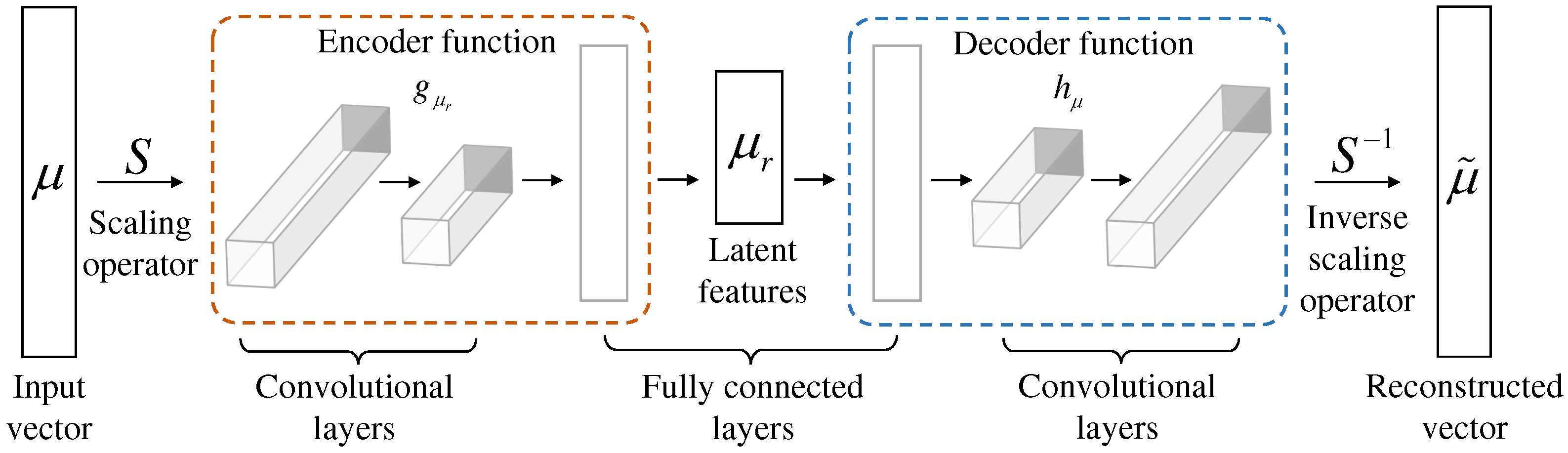For instance, when constructing a sampling database in a moderately sized design variable space ($N_{\mathcal{D}}\approx 20$), if only two parameter points are sampled per dimension—this being the minimum required to construct an interpolation database—it would require as many as $2^{20}=1,048,576$ sampling data points, which is computationally infeasible [1]. Many studies have found that multilayer auto-encoders, due to the neural network’s (NN) exceptional ability to capture nonlinear features, often outperform other nonlinear dimensionality reduction methods in various cases [27]. Researchers investigating the universal underlying NN structure for optimization problems with insensitive dependencies have found that, for PDE-based aerodynamic shape optimization problems, the most suitable auto-encoder should consist of two convolutional layers and one fully connected layer, as shown in Figure 2.

Boncoraglio and Farhat [1] proposed an efficient method for constructing the dataset, which involves quickly solving simplified models or simplified problems to record snapshots of the design space in the matrix $\mathbb{S}\in {\mathbb{R}}^{N_{\mu }\times N_{snapshot}}$. Small perturbations are then added to each dimension, and the final constructed training set $\mathbb{T}\in {\mathbb{R}}^{N_{\mu }\times N_{snapshot}(N_{\mu }+1)}$ is represented as Equation (8):

$$\mathbb{T}=\{{\left\{{\mu }_k\right\}}_{k=1}^{N_{snapshot}}\cup {\left\{{\mathbb{S}}_k\right\}}_{k=1}^{N_{snapshot}}\}$$

(8)

Here, ${\mathbb{S}}_k$ denotes the perturbation matrix corresponding to the k-th element in the snapshot matrix $\mathbb{S}$, as expressed in Equation (9). ${\mathbf{1}}^{1\times N_{\mu }}$ is a vector with all elements equal to 1, and ${\mathbf{I}}_{N_{\mu }}$ is the identity matrix; $ϵ$ is a small constant, such as $1\times {10}^{-3}$.

$${\mathbb{S}}_k={\mu }_k{\mathbf{1}}^{1\times N_{\mu }}+ϵ{\mathbf{I}}_{N_{\mu }}$$

(9)

The dataset is randomly split into a training set and a test set in an 8:2 ratio. The encoder network consists of two one-dimensional (1D) convolutional layers and one fully connected layer. The decoder has a structure that is symmetric to the encoder. More details of the auto-en/decoder can be found in reference [1], and the neural network structure parameters used in this study are referenced from that work. The original problem, as expressed in Equation (2), can be rewritten in the form of Equation (10).

$$\begin{array}{cc}\hfill \underset{{\mu }_r\in {\mathbb{R}}^{N_{{\mu }_r}}}{min}& f(q_r\left({\mu }_r\right),{\mu }_r)\hfill \\ \hfill \mathrm{subject}\mathrm{to}& c_r(q_r\left({\mu }_r\right),{\mu }_r)\le 0\hfill \end{array}$$

(10)

4. Aerodynamic Shape Optimization of uCRM-9 Wing

The objective of this optimization case was to minimize drag under lift and moment constraints for the uCRM-9 wing using the fast aerodynamic shape optimization design framework proposed in this work. In this section, we will provide a complete description of the problem. The calculations were performed using High-Performance Computing (HPC), with a single node based on the X86 architecture, featuring 64 cores, a 2.50 GHz clock speed, and 256 GB of RAM. All computations were conducted on this platform.

4.1. Baseline Geometry

In order to validate and compare different CFD solvers, NASA developed new benchmark geometry Common Research Model (CRM), which has been used in AIAA drag prediction since it was released in 2008 [28]. As a purely aerodynamic benchmark, the shape of the wing was designed with a deflection at its nominal 1 g flight condition, but the inherent deflection made it unsuitable for aeroelastic analysis and design optimization. Two undeflected Common Research Models (uCRMs) with different aspect ratios of 9 (uCRM-9) and 13.5 (uCRM-13.5) were released in 2018 by Brooks et al. [29] using the multidisciplinary design optimization (MDO) approach based on the NASA CRM. In this work, the uCRM-9 wing was selected as the optimization target, with its geometry shown in Figure 3 and

Table 1. CFD reference values and geometry specifications for the wing of uCRM-9.

	Quantity	Value
CFD reference values	Reference area	$594,720$ in. 2
	Mean aerodynamic chord	275.8 in.
	Moment reference	$(1325.90,0,177.95)$ in.
	Reynolds number $(M_{\infty }=0.85)$	$4.3\times {10}^7$
Geometry specifications	Aspect ratio	9.0
	Span	2313.4 in.
	Side of body chord	469.3 in.
	Tip chord	107.7 in.
	Gross area	638,756 in.2
	Exposed area	522,429 in.2
	1/4 chord sweep	35 deg
	Taper ratio	0.275

. The complete geometric files (https://mdolab.engin.umich.edu/wiki/ucrm (accessed on 16 March 2025)) (IGES/TIN) are provided in reference [29].

The flow environment for the optimization test case was taken from reference [29], with a flight altitude of 37,000 ft, $M_{\infty }$ = 0.85, and an angle of attack of $2.{044}^{\circ }$. The CFD boundary conditions are presented in

Table 2. CFD boundary conditions (37,000 ft).

	Boundary Type	Physical Property	Value
Wing	No-slip	Velocity	${\overrightarrow{v}}_{\mathrm{wall}}=0$
Symmetry plane	Symmetry		${\overrightarrow{v}}_{\mathrm{symm}}·\overrightarrow{n}$ = 0 *
Far field	Non-reflecting far-field	$M_{\infty }$	0.85
		Temperature	216.65 K
		Pressure	21731.1 Pa
		Angle of attack	2.044°

Far-field data come from the U.S. Standard Atmosphere, 1976 [30]. * $\overrightarrow{n}$ denotes the normal vector of the symmetry plane.

. Other geometric reference values are provided in Table 1.

4.2. Mesh Convergence Study

The present study employed a structured multiblock node-matching mesh with an O-H topology, and the far-field boundary was set at 50 times the mean aerodynamic chord (MAC) length, consistent with the reference grid provided in [29], as shown in Figure 4. Three meshes with varying coarsening levels are illustrated in Figure 5, with corresponding grid parameters provided in

Table 3. Mesh convergence study data.

Mesh Level	Chordwise Cells	Spanwise Cells	${\mathbf{y}}_{\mathbf{max}}^{+}$	Cell Number	${\mathit{C}}_{\mathit{l}}$	${\mathit{C}}_{\mathit{d}}$	${\mathit{Cm}}_{\mathit{y}}$
Coarse	50	102	$\sim 1.1$	1,536,708	0.6013	0.03981	−0.2631
Medium	68	137	$\sim 0.8$	3,046,689	0.6009	0.03926	−0.2600
Fine	86	204	$\sim 0.6$	7,785,981	0.6008	0.03881	−0.2575

. A detailed flow condition is presented in Section 4.1. The flow solver used was ADflow [31]. The flow solver used the second-order spatial discretization. Inviscid flux was evaluated by the Roe scheme [32]. ADflow utilized the approximate Newton–Krylov (ANK) algorithm to converge residual equations and acted as a globalization scheme for the full Newton–Krylov (NK) solver [33]. The flow solver determined convergence by monitoring the reduction in the $L_2$ norm of the flow field residuals until it reached a predefined threshold. Essential results were obtained through full-order simulations by solving the Reynolds-Averaged Navier–Stokes (RANS) equations. Based on the Navier–Stokes (NS) equation, the RANS equation assumed that the turbulence-related variables were the superposition of time-averaged and pulsating quantities. The three-dimensional compressible RANS equation in the domain $\Omega \in {\mathbb{R}}^3$ could be expressed in the form of Equation (11) in reference [34], where the conservative variables $\mathbf{Q}={[\rho ,\rho \mathbf{U},\rho E]}^T$, and $\mathbf{U}={[u,v,w]}^T$ contain the velocity components in the three directions in a Cartesian system of reference.

$${\displaystyle \frac{\partial }{\partial t}}{\int }_{\Omega }\mathbf{Q}d\Omega +{\int }_{\partial \Omega }({\mathbf{F}}_{\mathbf{c}}-{\mathbf{F}}_{\mathbf{v}})·ds=0$$

(11)

The convective and viscous fluxes are defined as Equation (12).

$${\mathbf{F}}_{\mathbf{c}}=\left[\begin{array}{c}\rho (\mathbf{U}-{\mathbf{U}}_{\mathbf{g}})\\ \rho \mathbf{U}⨂(\mathbf{U}-{\mathbf{U}}_{\mathbf{g}})+p\mathbf{I}\\ \rho E(\mathbf{U}-{\mathbf{U}}_{\mathbf{g}})+p\mathbf{U}\end{array}\right]{\mathbf{F}}_{\mathbf{v}}=\left[\begin{array}{c}0\\ {\tau }_{ij}\\ {\tau }_{ij}{u}_j+{\dot{q}}_i\end{array}\right]$$

(12)

where ${\mathbf{U}}_{\mathbf{g}}$ is the velocity of the moving domain $\Omega$, $\mathbf{I}$ is a $3\times 3$ identity matrix. The shear stress ${\tau }_{ij}$ and heat flux ${\dot{q}}_i$ are defined as Equation (13)

$$\begin{array}{cc}\hfill \tau & =\vartheta \left({\displaystyle \frac{\partial u_i}{\partial x_j}}+{\displaystyle \frac{\partial u_j}{\partial x_i}}-{\displaystyle \frac{2}{3}}{\displaystyle \frac{\partial u_k}{\partial x_k}}{\delta }_{ij}\right)\hfill \\ \hfill {\dot{q}}_i& ={\displaystyle \frac{\vartheta C_p}{Pr}}{\displaystyle \frac{\partial T}{\partial x_i}}\hfill \end{array}$$

(13)

For calorically perfect gas, $C_p=\gamma R/(\gamma -1)$; $\gamma =1.4$ for air in standard conditions; and Pr is the Prandtl number. In accord with Boussinesq approximation, the total viscosity $\vartheta$ is composed of the laminar viscosity ${\vartheta }^l$ and turbulence viscosity ${\vartheta }^T$ as

$$\vartheta ={\vartheta }^l+{\vartheta }^T$$

(14)

where ${\vartheta }^l$ is determined by Sutherland’s law and ${\vartheta }^T$ can be determined by various turbulence models. The Spalart–Allmaras (SA) [35] turbulence model was adopted to compute the turbulence viscosity ${\vartheta }^T$. The no-slip wall boundary condition was imposed on the solid wall. The far-field boundary was modeled as a non-reflective boundary condition, whereby Riemann invariants were used to calculate the flow variables at the border.

As shown in Figure 6, the drag convergence curve is linear and demonstrates a consistent trend. After weighing the trade-off between computational time and accuracy, the medium mesh was chosen for the optimization process.

4.3. Optimization Problem

To perform aerodynamic shape optimization, it was necessary to parametrize the geometric model. In this study, the Free-Form Deformation (FFD) volume approach was employed [24,36]. The geometric deformation was controlled by displacing 240 FFD control points in the z-direction, as illustrated in Figure 7. The twist angle was modified by altering the local angle of attack, thereby adjusting the aerodynamic loads on the wing. The optimization details are provided in

Table 4. Aerodynamic shape optimization problem.

	Function/Variable	Description	Quantity
Minimize	$C_d$	Drag coefficient
With respect to	$\theta$	Twist angle of wing	1
	z	FFD control point z-coordinates	240
		Total design variables	241
Subject to
Case 1	$C_l=0.6$	Lift coefficient constraint	1
	$C{m}_y\ge -0.26$	Moment coefficient constraint	1
Case 2	$C_l=0.5$	Lift coefficient constraint	1
	$C{m}_y\ge -0.20$	Moment coefficient constraint	1
	$t\ge 0.25t_{\mathrm{base}}$	Minimum thickness constraints	750
	$V\ge V_{\mathrm{base}}$	Minimum volume constraint	1
	$∆z_{\mathrm{TE},\mathrm{upper}}=-∆z_{\mathrm{TE},\mathrm{lower}}$	Fixed trailing-edge constraints	12
	$∆z_{\mathrm{LE},\mathrm{upper}}=-∆z_{\mathrm{LE},\mathrm{lower}}$	Fixed leading-edge constraints	12
		Total constraints	777

. In this study, two cases were employed to validate the ROM-based optimization design framework. The optimization objective was to minimize the drag coefficient $C_d$. For Case 1, the lift coefficient was constrained as $C_l=0.6$ with $C{m}_y\ge -0.26$, while for Case 2, the lift coefficient was constrained as $C_l=0.5$ with $C{m}_y\ge -0.2$. The local airfoil profile was modified by adjusting the displacement of FFD control points in the z-direction to satisfy the design objectives. Notably, 25 and 30 monitoring points were distributed chordwise and spanwise, respectively, to track thickness and volume variations. During the optimization process, the local thickness had to be at least one-quarter of the corresponding baseline thickness at each position, and the total volume had to be greater than that of the original baseline. When both twist and local shape variables were present, it was necessary to ensure that the local shape variables did not induce a shearing twist. This was conducted by constraining the upper and lower FFD control points on the leading and trailing edges to move in opposite directions [37].

4.4. Mesh Deformation

This study employed the Radial Basis Function (RBF) mesh deformation technique, which offers high accuracy, smooth deformation properties, and is independent of mesh type and topological structure. It is capable of handling large deformations and has been widely applied in optimization design and fluid–structure interaction (FSI) fields. The method achieved smooth mesh deformation by assuming that the surface mesh and volume mesh shared the same radial basis interpolation coefficients. The influence range of local displacements was controlled by the Radial Basis Function radius, denoted as $R_{RBF}$. The algorithmic principle is demonstrated by the formula in Section 3.3. In order to determine the optimal $R_{RBF}$ for the wing of uCRM-9, a heuristic method similar to the elbow method used in clustering was employed here [38]. A random deformation, ${\mu }_{random}\in \mathcal{D}$, was taken as the reference, and the error $e_{RBF}$ was defined as the maximum absolute error between the surface mesh points after RBF deformation and the reference deformation. The dimensionless Radial Basis Function radius ${\overline{R}}_{RBF}$ was given by ${\overline{R}}_{RBF}=R_{RBF}/\mathrm{MAC}$. As shown in Figure 8, by gradually increasing the dimensionless Radial Basis Function radius from 0.1 to 2.1, the error first decreased and then increased. When ${\overline{R}}_{RBF}$ was small, the range of local deformation influence was limited, and the deformation could not be effectively propagated, resulting in a larger error. When ${\overline{R}}_{RBF}=1.1$, the error was minimized, and this value was adopted for the subsequent optimization problems. If ${\overline{R}}_{RBF}$ continued to increase, the range of local deformation influence became too large, leading to the excessive smoothing of the overall deformation and resulting in a larger error.

To control geometric deformation through Free-Form Deformation (FFD), it is necessary to embed the mesh data points into the FFD box. A common approach is to directly embed the CFD surface mesh as a dataset into the control volume [37]. For models with a large number of surface mesh cells, selecting all cells would lead to significant computational overhead when transferring geometric deformation to the volume mesh using the RBF mesh deformation algorithm. Therefore, this study employed a greedy algorithm to reduce the number of surface deformation control points during mesh deformation. This approach minimized the computational cost of deformation transfer while ensuring accuracy, thus further accelerating the optimization design process. As shown in Figure 9, when the number of control points was relatively small, they were evenly distributed. As the number of control points increased, the distribution became denser in areas prone to larger deformations. For areas with local refinement, such as the wing trailing edge, this approach effectively prevented control points from clustering, thereby enhancing the numerical stability of the computation. Figure 10 demonstrates that when the number of selected points reached 3000, the error could be controlled within 1 $\times {10}^{-4}$. Compared to the baseline, where the RBF interpolation function was computed using all points, the computation time was reduced to 38.7% of the original time after point selection. Considering both accuracy and time cost, the subsequent optimization of the mesh deformation problem employed 3000 control points.

4.5. Optimizer

The optimizer in the aerodynamic shape optimization design framework based on a ROM was implemented using the pyOptSparse [39] framework, with the optimization algorithm employing SLSQP [40]. Constrained nonlinear optimization problems could be effectively solved with pyOptSparse, which offers a consistent interface for various gradient-based and gradient-free optimization algorithms. The ROM-based optimization framework solved the gradient using the finite difference (FD) method, thereby avoiding the computationally expensive process of solving the adjoint equations. This optimizer framework provided flexibility in the optimization process by directly targeting the needs of engineering optimization tasks. It was designed to minimize the objective function while simultaneously managing both equality and inequality constraints. The pyOptSparse optimizer framework was extensively validated through various applications [41,42,43,44,45].

5. Results

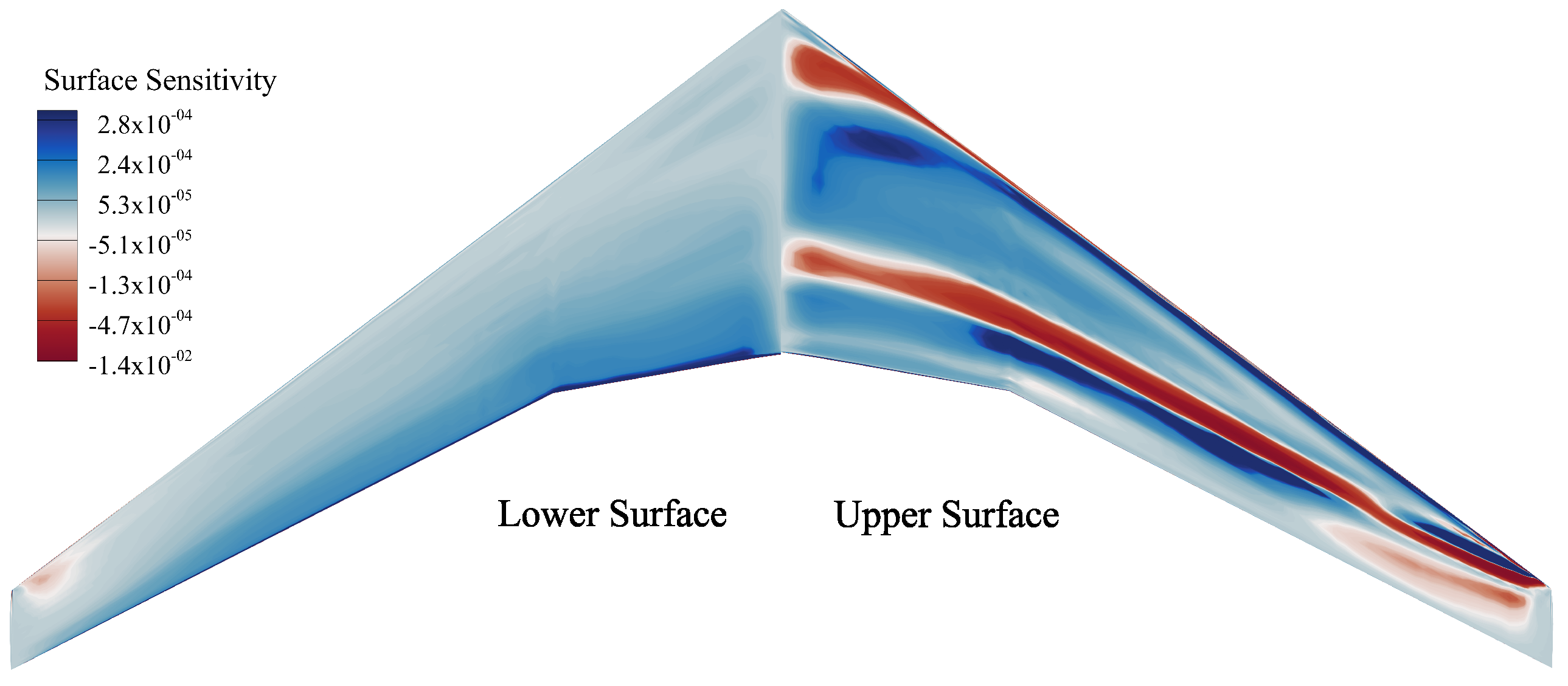
A priori sampling is a crucial element in the design of experiments (DoE), involving the systematic selection of samples from within the design space. This study employed a multi-round greedy Latin Hypercube Sampling (LHS) method to construct the sample space. In order to qualitatively assess, to some extent, the design variables that had a significant impact on the optimization objective function and constraints, surface sensitivity analysis was conducted first, as shown in Figure 11. From the contour plot of the sensitivity of the objective function with respect to the displacement in the z-direction, it can be observed that the design space regions with a significant impact on aerodynamic performance were concentrated near the shock wave occurrence location.

The sampling process was as follows:

• The initial design space samples were generated using LHS based on surface sensitivity information.
• The surface pressure coefficient $C_p$ was extracted from FOM simulations to construct the test dataset and the initial sample space.
• The ROM was constructed using the sample space and was then employed to reconstruct the test dataset.
• The design variables with larger errors were identified by comparing the discrepancies between the predicted reconstruction results and the FOM $C_p$ distribution.
• Additional sampling points were introduced in the dimensions of design variables with larger errors. Each new sample was evaluated to ensure compliance with geometric constraints. If the constraints were satisfied and no negative volume errors were introduced in the mesh, the sample was added to the sample space; otherwise, it was discarded.
• The above process was repeated for the next round of sampling.

The accuracy of ROMs typically increases with the expansion of the sample space, highlighting the iterative process of model improvement. A total of four rounds of DoE were conducted, with the test datasets existing independently. The arithmetic mean of the error between the predicted reconstruction results and the FOM distribution $C_p$ was defined as the iterative criterion. Starting from the initial samples, the DoE samples were gradually increased, and the error was reassessed in each iteration. This process was repeated until the error reached an acceptable threshold. Each round targeted 100 data points; points that did not satisfy the constraints or caused severe grid negative volume errors were discarded. A total of 331 data points were used to construct the database. It is noteworthy that the database could also be shared as an input for the active manifold network. The sampling process prioritized design variables based on their impact on aerodynamic performance by evaluating the ROM prediction errors. For aerodynamic optimization applications, it is particularly crucial to construct the test dataset based on surface sensitivity analysis. This ensures the accurate prediction of aerodynamic loads during the optimization process while avoiding unnecessary sampling costs.

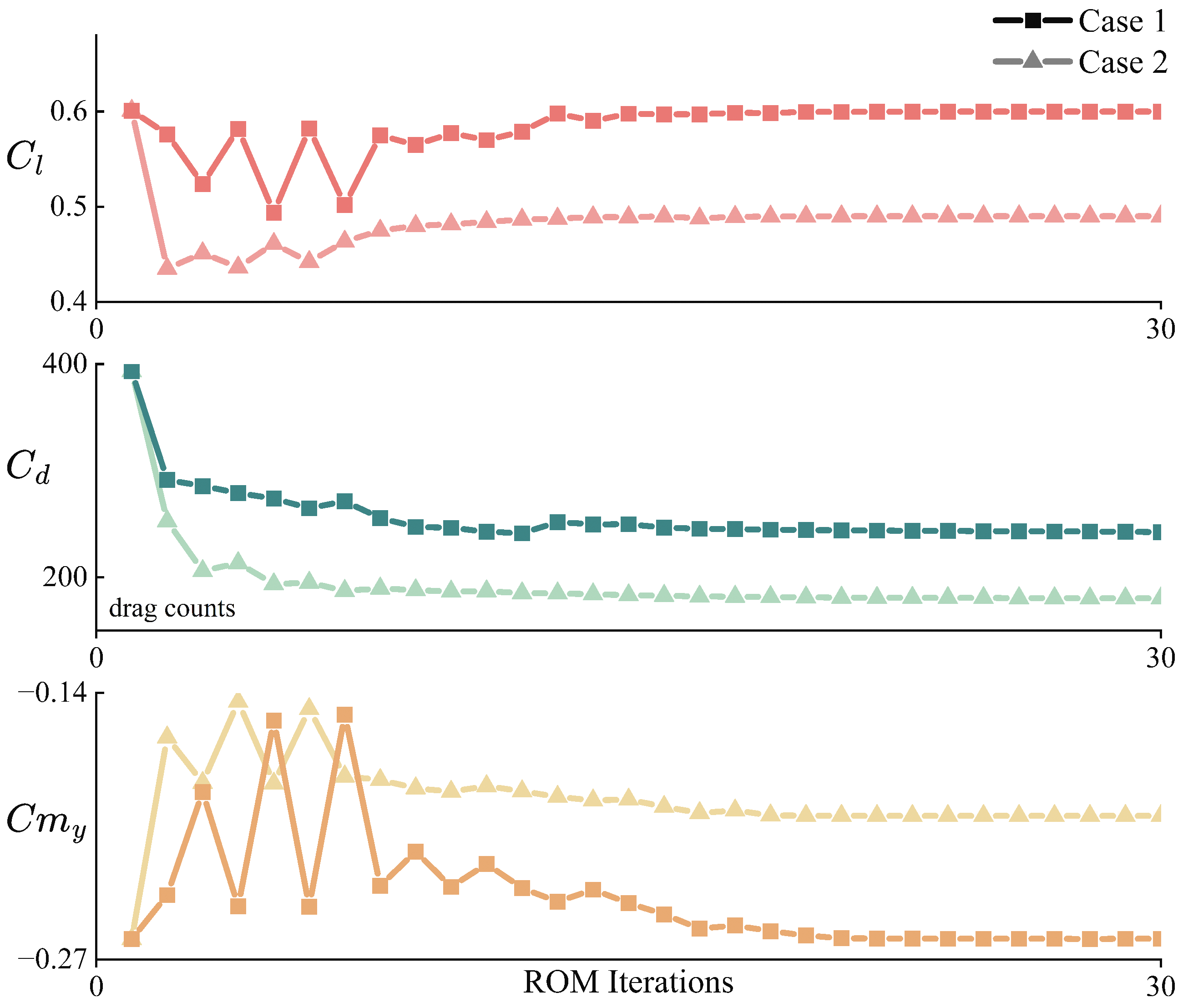
As shown in Figure 12, after 20 iterations, the objective function essentially converged, and the constraints reached the preset values.

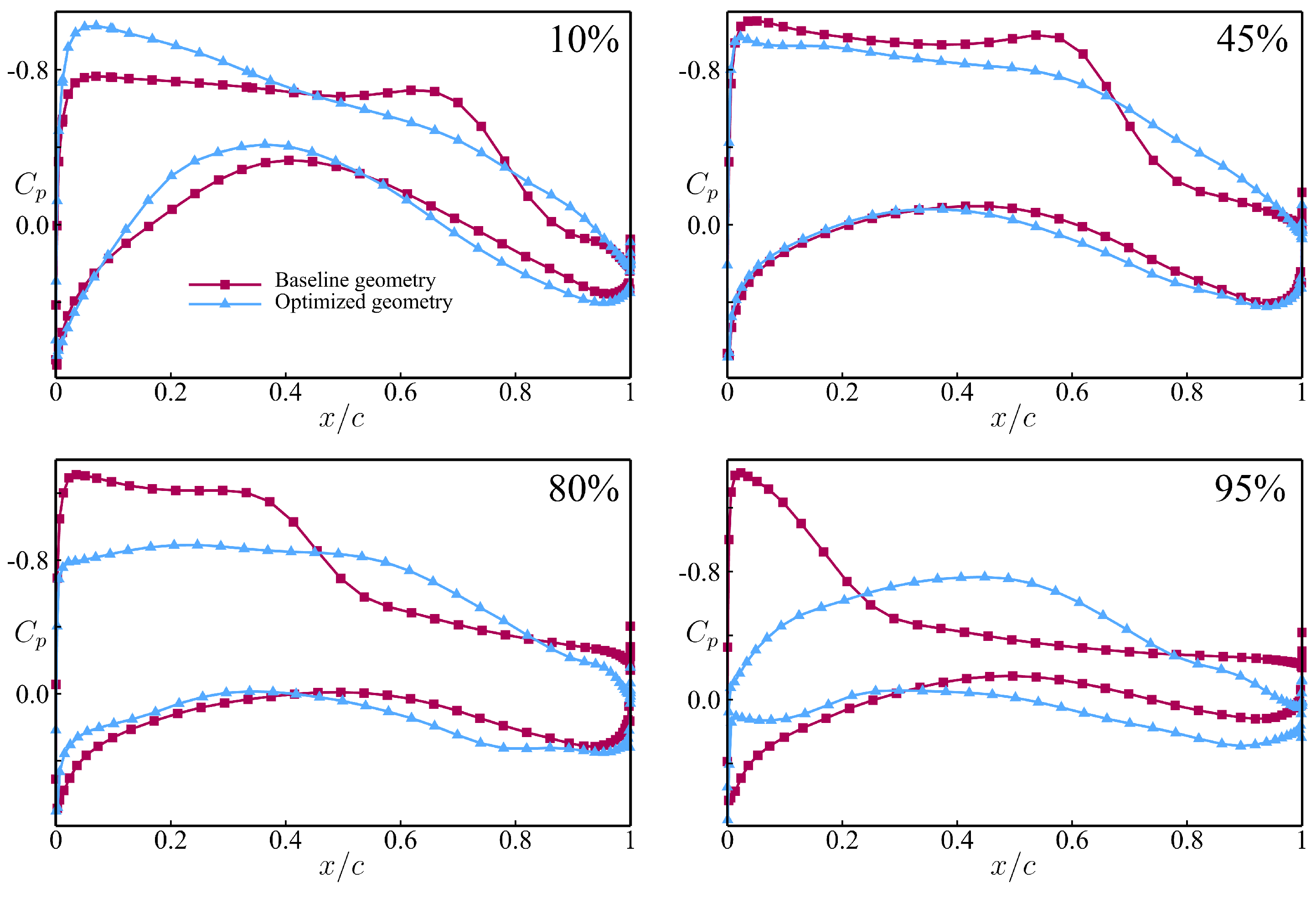
As shown in Figure 13, the change in wing thickness and the alteration in the twist angle led to a change in the local angle of attack, causing the shockwave position on the wing surface to shift. The shockwave on the upper surface moved towards the wing root. The local aerodynamic profile modification suppressed the shockwave diffusion, reducing the pressure drag. From the contour plots, it can be observed that the optimized wing exhibited a reduced shock wave region and decreased shock intensity. The optimized wing exhibited a delayed critical Mach number. In the mid-span section, the sectional load distribution indicated a reduction in shock intensity, with this trend becoming more pronounced toward the wingtip. The local aerodynamic load was more evenly distributed, and peak values were significantly reduced. Flow discontinuities disappeared, leading to an effective reduction in pressure drag. Ultimately, the drag coefficient decreased by 38.9%. Pressure coefficients were extracted at 10%, 45%, 80%, and 95% spanwise locations, as shown in Figure 14. The optimized wing exhibited significant differences in pressure coefficients across the entire wing surface compared to the baseline geometry.

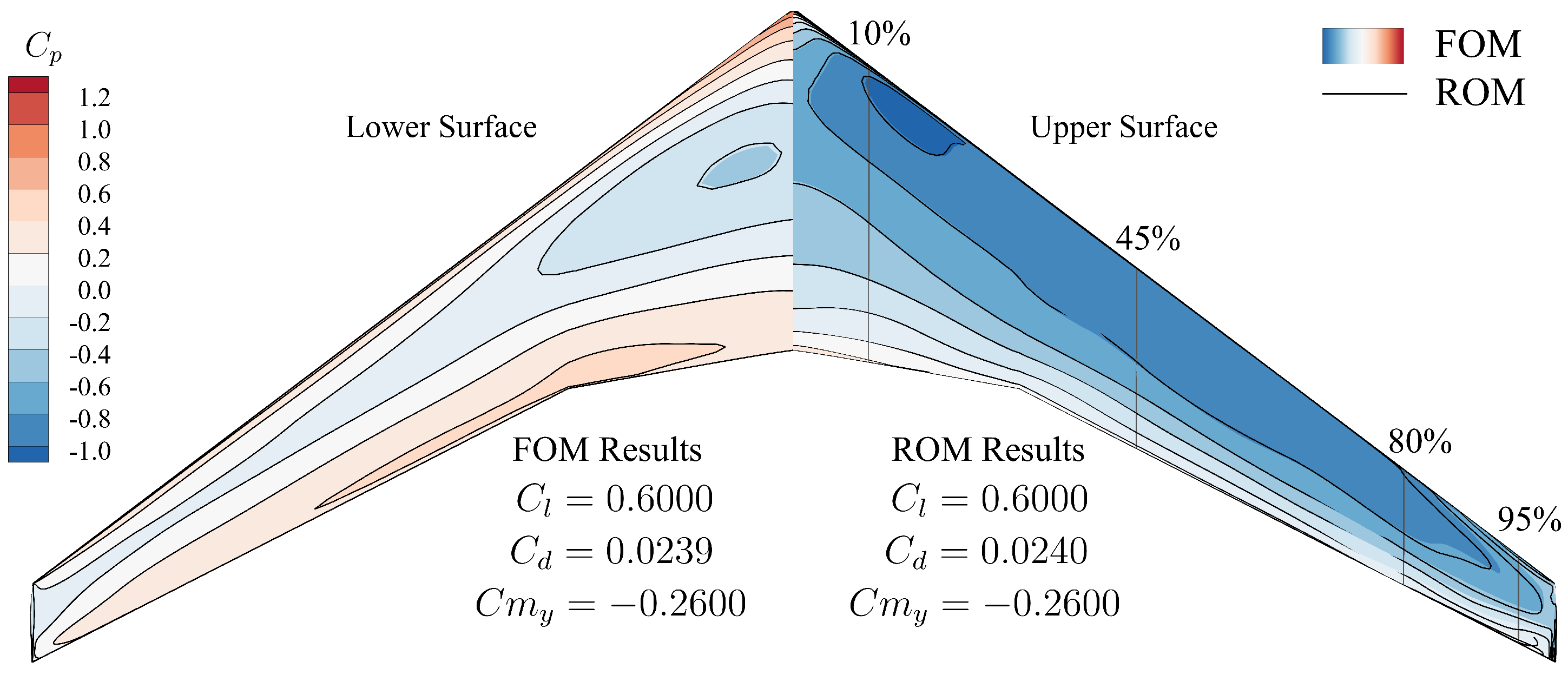
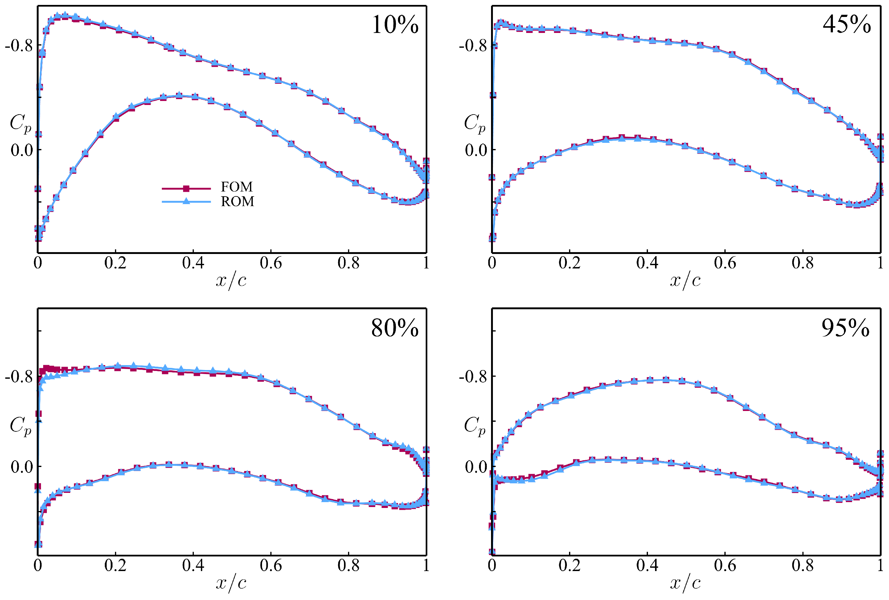
To further assess the accuracy of the ROM-based optimized design framework, the optimization results were compared with those obtained from the FOM-based optimization design framework. The concentrated aerodynamic loads are obtained by solving the RANS equations, while the design variable gradients were derived by solving the adjoint equations. As shown in Figure 15, the optimization design framework based on ROM demonstrated high accuracy, with results that were nearly consistent with those from the FOM-based framework. By extracting sections in different spanwise locations, it could be observed that the local pressure coefficients aligned well, as shown in Figure 16.

Table 5. Performance and resource usage comparison of FOM- and ROM-based optimization.

		Case 1		Case 2
Component	Process Details	$\mathbf{ROM}$	FOM	$\mathbf{ROM}$	FOM
Building framework	Wall-clock time	9 h 23 min		7 h 15 min
Optimization		1.6 min	25 h 8 min	1.3 min	17 h 12 min
Total time	t/$t_{\mathrm{FOM}}$	$37.4\%$	$100.0\%$	$42.3\%$	$100.0\%$
Objective function	$C_d\left(\mathrm{counts}\right)$	240	239	179	179
$C_d$ reduction	$|C_d^{\mathrm{Base}}-C_d^{\mathrm{Opt}}|/C_d^{\mathrm{Base}}$	$38.9\%$	$39.2\%$	$54.5\%$	$54.5\%$

compares the computational resource consumption between the ROM-based and FOM-based optimization frameworks. It can be observed that although the primary computational cost of the ROM-based optimization was concentrated in the building phase, the absence of the need to solve the computationally expensive adjoint equations led to a 62.6% reduction in the overall optimization time. This time was significantly lower than that of the FOM-based optimization framework, with the final optimization result exhibiting an error of 0.3%, demonstrating its high practical applicability.

Test Case 2 was employed to validate the generalization capability of the aerodynamic shape optimization framework proposed in this study for different problems. The details of the optimization setup are presented in Table 4. The optimization objective was to minimize the drag coefficient $C_d$, while maintaining $C_l=0.5$ and ensuring that $C{m}_y\ge -0.20$. 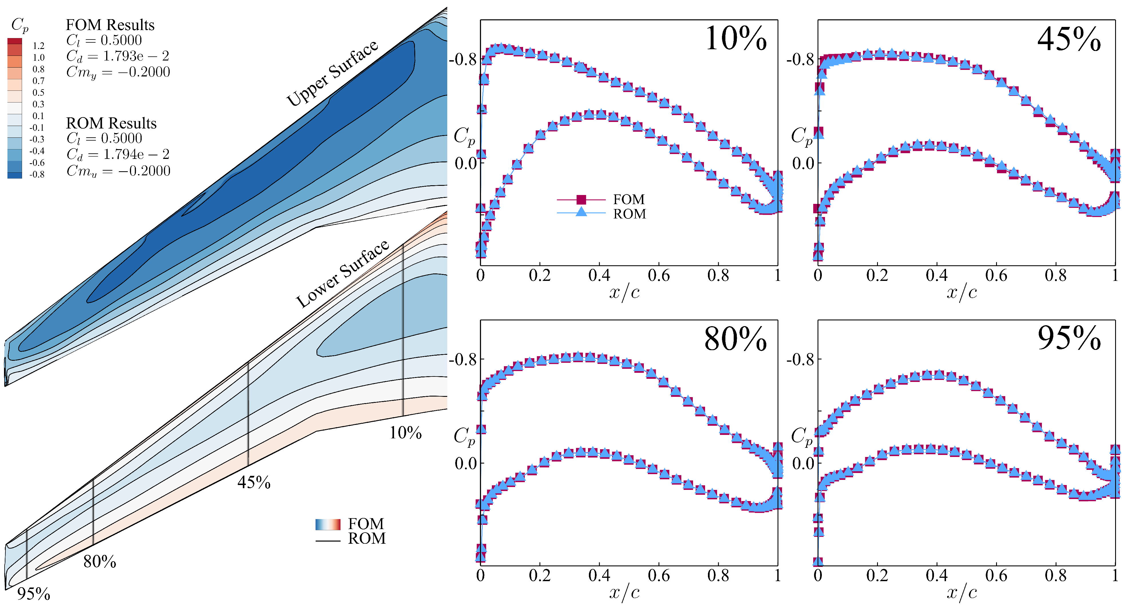The optimization process is illustrated in Figure 12. As illustrated in Figure 17, the newly developed rapid aerodynamic shape optimization framework based on the ROM demonstrated high accuracy. The drag coefficient was reduced by 54.5%, and the total computational resource consumption was decreased by 57.7%, as summarized in Table 5.

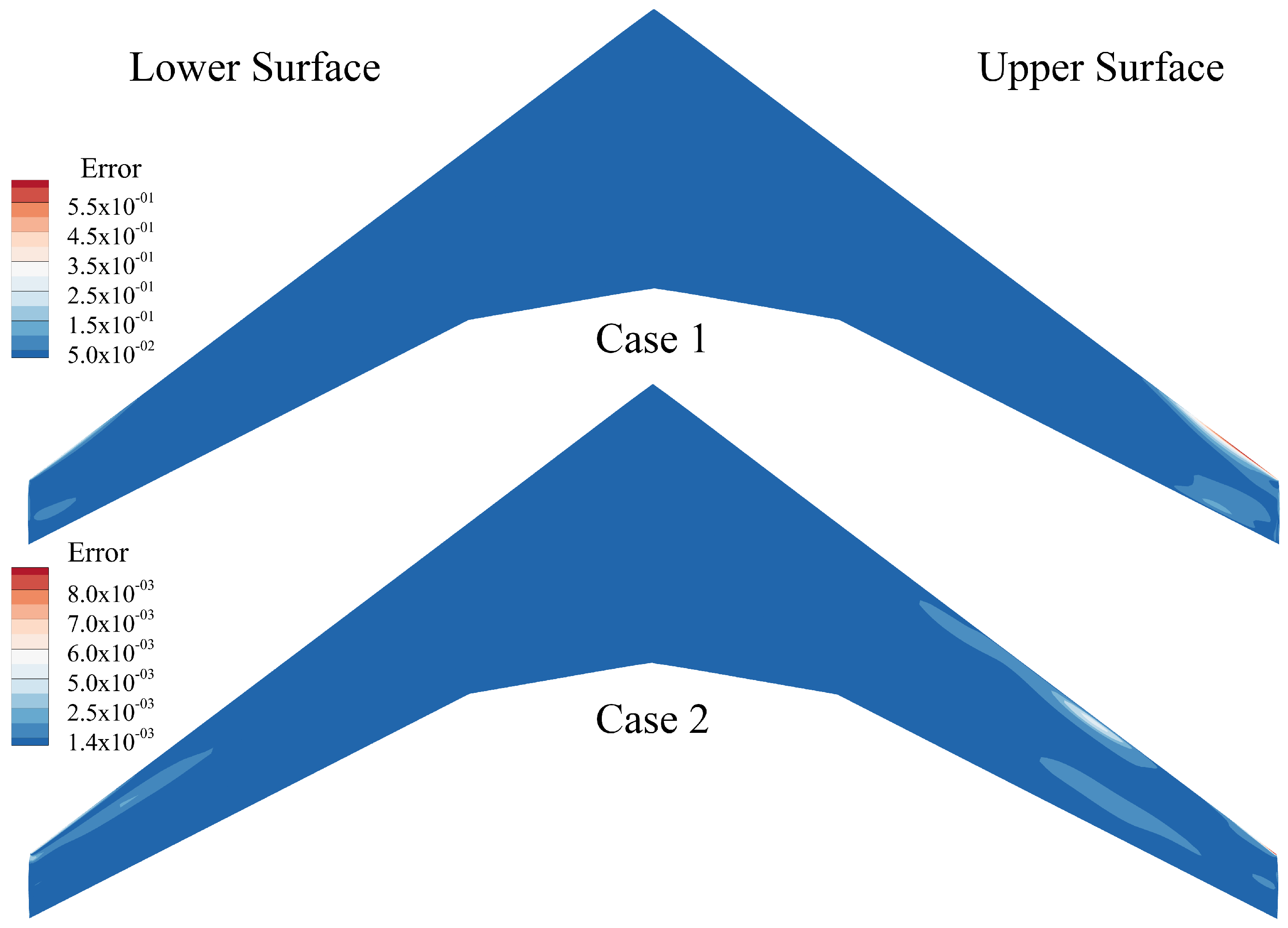
As shown in Figure 18, the error was defined as the absolute difference in $C_p$ between the ROM-based framework and the FOM-based framework optimization results. By comparing the contour plots, it can be observed that the errors in Case 1 and Case 2 were primarily concentrated near the wingtip. This was due to the increasing coupling effect between the twist angle and thickness design variables as the wingtip was approached. In contrast, near the wing root, the twist angle design variable had a relatively smaller impact, while the thickness design variable played a dominant role. As a result, most of the errors in the wing root and mid-span regions remained within a relatively small range.

6. Conclusions

This work presents a fast aerodynamic shape optimization design framework based on the LLE+COGA reduced-order model. By constructing an active manifold auto-en/ecoder neural network, the framework eliminates the unacceptable computational costs associated with high-dimensional design spaces. This study finds that for surface grids with a large number of locally refined regions, the computational expense of transferring geometric deformations from the surface grid to the volume grid via mesh deformation algorithms is substantial. To address this, a greedy point selection algorithm is proposed, which reduces the computation time by 71.3% while maintaining an error accuracy below 1 $\times {10}^{-4}$. The proposed ROM-based framework was validated through the drag reduction optimization of the UCRM9 wing, which involved 241 design variables and 777 constraints. Ultimately, under the given constraint conditions, the drag reduction achieved for Case 1 and Case 2 was 38.9% and 54.5%, respectively, which was consistent with the results obtained using the FOM-based optimization framework. The total optimization time for Case 1 and Case 2 was reduced by 62.6% and 57.7%, respectively, demonstrating the high practical value of the ROM-based optimization framework proposed in this study.