Direct Numerical Simulation of Boundary Layer Transition Induced by Roughness Elements in Supersonic Flow

Abstract

Current research on the transition mechanisms induced by moderate-height roughness elements remains insufficiently explored. Hence, direct numerical simulation (DNS) and BiGlobal stability analysis are employed in this study to investigate boundary layer transition from laminar to turbulent flow induced by moderate-height isolated roughness elements and roughness strips under a supersonic freestream at Mach 3.5. Analysis of DNS results reveals that the isolated roughness element induces transition within the boundary layer, characterized by two high-speed streaks in the wake. This transition is attributed to the coupling between the separated shear layer at the roughness apex and the downstream counter-rotating vortex pair (CVP). BiGlobal stability analysis further identifies that symmetric eigenmodes dominate the transition process in the wake, actively promoting flow destabilization. Conversely, the roughness strip configuration suppresses transition, with only attenuated high-speed streaks persisting in the near wake before complete dissipation. The wake flow exhibits multiple CVPs and adjacent horseshoe vortex pairs interacting with the shear layer, with antisymmetric modes dominating this process. These findings provide technical foundations and theoretical frameworks for predicting and controlling roughness-induced transition.

1. Introduction

The laminar–turbulent transition mechanism on supersonic vehicle surfaces represents a critical research focus in fluid dynamics and aerospace engineering, owing to its profound implications for predicting and regulating aerodynamic drag, thermal loading and skin friction characteristics [1,2,3]. This transition constitutes a multifaceted flow process governed by nonlinear interactions, with roughness-induced destabilization emerging as a pivotal strategy for active flow control [4,5]. The strategic implementation of surface-mounted roughness elements or optimized distributed roughness arrays enables the targeted manipulation of boundary layer dynamics, accelerating laminar-to-turbulent transition to enhance wall shear stress and convective heat-transfer rates—a capability essential for specialized aerodynamic configurations and thermal management systems [6,7]. Recent advancements in roughness-mediated transition studies have intensified the demand for a fundamental understanding of how localized surface perturbations modulate boundary layer stability thresholds and disturbance-amplification pathways [8,9].

The laminar-to-turbulent transition dynamics governed by surface roughness are critically dependent on geometric parameters, including roughness height $\mathit{k}$, shape morphology and configuration (isolated elements versus distributed strips). A key dimensionless parameter governing transition onset is the relative roughness height $k/\delta$, defined as the ratio of roughness height $\mathit{k}$ to boundary layer thickness $\delta$. Classification distinguishes three regimes: subcritical ($k/\delta \ll 1$), moderate ($k/\delta \approx 1/2$) and critical ($k/\delta \approx 1$) roughness scales [10]. In supersonic flows interacting with moderate roughness elements, the boundary layer develops intricate flow features, including upstream separation zones preceding the roughness element; oblique shock formation at the roughness apex; wake vortical structures with embedded counter-rotating vortex pairs (CVPs); and shear layer detachment downstream of the roughness element [11,12]. These interconnected flow components engage in nonlinear interactions within the roughness wake, collectively destabilizing the boundary layer and precipitating transition through modal amplification mechanisms.

Extensive experimental and computational investigations have elucidated the perturbation mechanisms induced by surface roughness in supersonic boundary layers. Bartkowicz et al. [13] performed wind tunnel experiments at Mach 6, demonstrating that vortical structures originating from upstream separation zones instigate turbulent transition in roughness wakes. Casper et al. [14] employed temperature-sensitive coatings to identify thermal streak formation downstream of roughness elements, which subsequently evolve into vortical disturbances modulating near-wall flow dynamics. Wang et al. [15] experimentally validated that surfaces with distributed roughness elements exhibit enhanced susceptibility to boundary layer transition compared to smooth flat plates. High-fidelity direct numerical simulation (DNS) performed by Kurz et al. [16] resolved the genesis of horseshoe vortices flanking roughness elements and wake recirculation zones containing CVPs, whose synergistic interactions generate crossflow vortices that destabilize the boundary layer. Bernardini et al. [17] established that roughness-induced separated shear layers exhibit instability at critical roughness Reynolds numbers ($R{e}_k$), triggering hairpin vortex shedding and turbulent breakdown. Subbareddy et al. [18] quantified the spatiotemporal intermittency of horseshoe vortices and shear layer oscillations, linking their high unsteadiness to incipient turbulent fluctuations. De et al. [19] identified dominant CVP structures in roughness wakes that amplify shear layer instabilities, culminating in turbulence onset. Shrestha et al. [20] emphasized the critical coupling between apex-separated shear layers and downstream CVPs as a transition catalyst. Liu et al. [21] further validated this mechanism via DNS and BiGlobal stability analysis, revealing that symmetric eigenmodes of CVPs exhibit superior disturbance growth rates, thereby dominating transition initiation. Collectively, these studies underscore the predominance of symmetric modal instabilities in roughness-mediated transition processes.

Investigations into roughness strip-induced boundary layer transition have identified critical dependencies on geometric scaling parameters. Whitehead et al. [22] performed Mach 6.8 wind tunnel experiments to evaluate the role of the dimensionless spacing ratio $S/W$ (spanwise element spacing S to element width W) in transition modulation. Their findings revealed that transition remains weakly influenced at $S/W\ge 3$, where minimal vortex interference occurs between adjacent elements. However, for $S/W<3$, intensified vortical interactions between closely spaced elements induce a systematic downstream migration of transition onset—a phenomenon corroborated by Shrestha et al. [23], who observed transition stabilization at $S/W\approx$ 3–4, but significant downstream displacement at $S/W<3$, where roughness strips function as aerodynamic barriers rather than discrete vortex generators. Subsequent studies by Shrestha et al. [24] and Schneider et al. [25] employed power spectral density (PSD) analysis to characterize dominant wake frequencies and transient flow features in large-scale roughness arrays ($k/\delta \ge 1$), though the mechanistic links between $S/W$ and transition dynamics remain underexplored. Semper et al. [12] and Shrestha et al. [20] further demonstrated that at $S/W=2$ and $k/\delta \approx 1.33$, upstream vortex shedding dominates wake destabilization, directly precipitating transition. Gilles et al. [26] demonstrated through experimental studies on miniature vortex generators that an increase in the height of the miniature vortex generators leads to enhanced circulation and larger vortex core radii. Huang et al. [27] employed DNS to investigate boundary layer transition characteristics under roughness strips of varying heights, revealing that transition is triggered by high-height roughness strips, while no transition occurs under low-height roughness strips. Liu et al. [28] studied two moderately spaced roughness elements and observed the formation of CVPs between two adjacent roughness elements. As the boundary layer develops streamwise, it gradually becomes unstable; the interaction between these vortices generates vortex legs, which further evolve into hairpin vortices, serving as the primary source of turbulent kinetic energy. Liu et al. [29] investigated the flow characteristics and transition mechanisms under the influence of several differently shaped roughness elements, further confirming that transition is caused by interactions between CVPs and the boundary layer, while also demonstrating that the shape of roughness elements influences the location of transition onset. Despite comprehensive insights into large roughness elements ($k/\delta \ge 1$), the transitional physics governing moderate-scale roughness configurations ($0.5<k/\delta <1$) remain poorly characterized. This study addresses this knowledge gap by systematically analyzing flow mechanisms in roughness strips operating within this intermediate regime.

Previous studies have demonstrated that roughness elements can induce boundary layer transition through flow perturbations. However, existing research predominantly focuses on large-scale roughness elements, while the transition mechanisms and the differences of mechanism between isolated roughness elements and roughness strips remain inadequately explored. This study therefore systematically investigates the transition mechanisms induced by moderate-height roughness elements and strips in a Mach 3.5 supersonic flow, with particular emphasis on delineating their distinct transition pathways. DNS were conducted to resolve the flow fields perturbed by both configurations. The analysis protocol initiates with characterization of fundamental flow structures to identify the primary instability sources within their respective wakes, culminating in BiGlobal stability analysis to elucidate the dominant instability modes governing wake evolution.

This paper is structured as follows: Section 2 details the numerical framework, including governing equations and discretization schemes. Section 3 specifies the geometric configurations of roughness elements/strips and computational domain boundary conditions. Furthermore, mesh-independent studies are analyzed. Section 4 presents a multi-scale analysis of the baseline flow topology, followed by a focused examination of wake instability mechanisms for both roughness configurations. Section 5 conclusively synthesizes the principal findings of this investigation, delineates the methodological approaches employed and provides perspectives for future research directions.

2. Numerical Methods

2.1. Navier–Stokes Equations

The mathematical foundation of this investigation adopts the three-dimensional, time-accurate Navier–Stokes (NS) equations to govern compressible flow dynamics. These equations, expressed in their conservation form, are formulated as follows:

$${\displaystyle \frac{\partial \mathit{Q}}{\partial t}}+{\displaystyle \frac{\partial {\mathit{F}}_j^c}{\partial x_j}}={\displaystyle \frac{\partial {\mathit{F}}_j^v}{\partial x_j}}(j=1,2,3)$$

(1)

where t designates the temporal dimension, while $x_j$ defines the orthogonal spatial coordinates along the j-axis. The governing system is characterized by three primary tensorial quantities: the conserved variable vector $\mathit{Q}$, the inviscid flux tensor ${\mathit{F}}_{\mathit{j}}^{\mathit{c}}$ and the viscous flux tensor ${\mathit{F}}_{\mathit{j}}^{\mathit{v}}$. These terms are rigorously defined as follows:

$$\mathit{Q}=\left[\begin{array}{c}\rho \\ \rho u_i\\ \rho e\end{array}\right],{\mathit{F}}_j^c=\left[\begin{array}{c}\rho u_j\\ \rho u_i{u}_j+p{\delta }_{ij}\\ (\rho e+p)u_j\end{array}\right],{\mathit{F}}_j^v=\left[\begin{array}{c}0\\ {\sigma }_{ij}\\ {\sigma }_{ij}{u}_i+q_j\end{array}\right]$$

(2)

and

$$e={\displaystyle \frac{p}{(\gamma -1)\rho }}+{\displaystyle \frac{u_i^2}{2}}$$

(3)

$${\sigma }_{ij}=\mu \left({\displaystyle \frac{\partial u_j}{\partial x_i}}+{\displaystyle \frac{\partial u_i}{\partial x_j}}\right)-{\displaystyle \frac{2}{3}}\mu {\delta }_{ij}\nabla ·\mathit{u}$$

(4)

$$q_j=k{\displaystyle \frac{\partial T}{\partial x_j}}$$

(5)

where ${\mathit{\sigma }}_{ij}$ represents the Kronecker delta function, while the velocity vector $u={[u,v,w]}^T$ defines the flow field in Cartesian coordinates. The thermodynamic properties include the thermal conductivity k, static pressure p and fluid density $\rho$. The dynamic viscosity $\mu$ is determined through Sutherland’s viscosity law, which accurately models temperature-dependent viscous effects in compressible flows. The system of governing equations is completed by the ideal gas state equation, expressed as follows:

$$k={\displaystyle \frac{\gamma c_p}{P_r}},\mu ={\displaystyle \frac{a{T}^{1.5}}{T+b}},p=\rho RT$$

(6)

The Sutherland’s law coefficients are specified as $a=1.458\times {10}^{-6}$ $\mathrm{Pa}·\mathrm{s}$ and $b=110.4$ $\mathrm{K}$. The thermodynamic properties include the specific heat ratio $\gamma =1.4$, gas constant $R=287$ $\mathrm{J}/(\mathrm{kg}·\mathrm{K})$ and Prandtl number $P_r=0.72$. Velocity components u, v and w are normalized by the freestream velocity $u_{\infty }$, while other flow variables are scaled using their corresponding freestream reference values. The characteristic length scale for normalization is $L_{ref}$ = 0.001 m.

The numerical framework employs a curvilinear coordinate-aligned mesh system for solving the governing Navier–Stokes equations, utilizing a high-precision finite-difference algorithm derived from the OpenCFD library’s DNS suite by Li [30] (https://opencfd.cn/). Temporal integration is achieved through a three-stage third-order Runge–Kutta temporal integration scheme [31]. Spatial discretization of convective terms combines a seventh-order weighted essentially non-oscillatory (WENO-SYMBO) reconstruction with Steger–Warming flux vector splitting to ensure shock-capturing fidelity [32,33]. Diffusive flux components are resolved via an eighth-order centered differencing operator, maintaining spectral-like accuracy in viscous-dominated regions.

2.2. BiGlobal Stability Analysis

For stability analysis of the flow field, the primitive variables in the Navier–Stokes equations are decomposed into a steady base flow and a small perturbation. This decomposition separates the flow field into a time-invariant component and a small-amplitude disturbance, enabling the study of flow stability characteristics.

$$\mathit{q}(x,y,z,t)=\overline{\mathit{q}}(x,y,z)+{\mathit{q}}^{\prime }(x,y,z,t)$$

(7)

where $\overline{\mathit{q}}$ denotes the steady base flow field, while ${\mathit{q}}^{\prime }$ characterizes the infinitesimal perturbation field, with the perturbation amplitude constrained by $\left|{\mathit{q}}^{\prime }\right|<\left|\overline{\mathit{q}}\right|$. Through substitution of Equation (7) into the Navier–Stokes formulation (1) and subsequent linearization about the base flow solution, the governing equations for perturbation dynamics are derived. This linearization process, which neglects higher-order nonlinear terms, yields the linearized Navier–Stokes (LNS) equations governing small-amplitude disturbance evolution.

$$\begin{array}{c}\mathbf{\Gamma }{\displaystyle \frac{\partial {\mathit{q}}^{\prime }}{\partial t}}+\mathit{A}{\displaystyle \frac{\partial {\mathit{q}}^{\prime }}{\partial x}}+\mathit{B}{\displaystyle \frac{\partial {\mathit{q}}^{\prime }}{\partial y}}+\mathit{C}{\displaystyle \frac{\partial {\mathit{q}}^{\prime }}{\partial z}}+\mathit{D}{\mathit{q}}^{\prime }\hfill \\ ={\mathit{H}}_{xx}{\displaystyle \frac{{\partial }^2{\mathit{q}}^{\prime }}{\partial x^2}}+{\mathit{H}}_{yy}{\displaystyle \frac{{\partial }^2{\mathit{q}}^{\prime }}{\partial y^2}}+{\mathit{H}}_{zz}{\displaystyle \frac{{\partial }^2{\mathit{q}}^{\prime }}{\partial z^2}}+{\mathit{H}}_{xy}{\displaystyle \frac{{\partial }^2{\mathit{q}}^{\prime }}{\partial x\partial y}}+{\mathit{H}}_{xz}{\displaystyle \frac{{\partial }^2{\mathit{q}}^{\prime }}{\partial x\partial z}}\hfill \\ +{\mathit{H}}_{yz}{\displaystyle \frac{{\partial }^2{\mathit{q}}^{\prime }}{\partial y\partial z}}\hfill \end{array}$$

(8)

The matrices $\mathbf{\Gamma }$, $\mathit{A}$, $\mathit{B}$, $\mathit{C}$, $\mathit{D}$, ${\mathit{H}}_{xx}$, ${\mathit{H}}_{yy}$, ${\mathit{H}}_{zz}$, ${\mathit{H}}_{xy}$, ${\mathit{H}}_{xz}$ and ${\mathit{H}}_{yz}$ are uniquely determined by the steady base flow variables. These matrices represent various operations and transformations applied to the perturbation quantities in the LNS equation, and they play a pivotal role in the linear stability analysis. Specifically, $\mathbf{\Gamma }$ incorporates thermodynamic properties of the base flow, including density and pressure. $\mathit{A}$, $\mathit{B}$, $\mathit{C}$ and $\mathit{D}$ correspond to the convective flux Jacobians derived from the velocity field. ${\mathit{H}}_{xx}$, ${\mathit{H}}_{yy}$ and ${\mathit{H}}_{zz}$ represent second-order spatial derivatives of the velocity components, constituting the diagonal terms of the Hessian tensor. ${\mathit{H}}_{xy}$, ${\mathit{H}}_{xz}$ and ${\mathit{H}}_{yz}$ quantify cross-derivative interactions, encapsulating shear-induced momentum transfer and three-dimensional flow coupling. For flows exhibiting pronounced wall-normal and spanwise gradients with weak streamwise variation, the quasi-parallel flow hypothesis is invoked to simplify stability analyses. Under this assumption, disturbance equations are reduced to a spatially parabolic form. Substituting the perturbation ansatz into the LNS equations yields a linear eigenvalue problem, from which modal growth rates and decay characteristics are extracted. The disturbance field is conventionally expressed as [34]:

$${\mathit{q}}^{\prime }(x,y,z,t)=\widehat{\mathit{q}}(y,z)exp(\mathrm{i}\alpha x-\mathrm{i}\omega t)+{\mathrm{c}}_{.}{\mathrm{c}}_{.}$$

(9)

In this equation, x denotes the streamwise direction, while $\widehat{\mathit{q}}$ characterizes the spatial structure of the disturbance mode. $\omega$ is the angular frequency. The complex streamwise wavenumber $\alpha ={\alpha }_r+\mathrm{i}{\alpha }_i$ encapsulates both the spatial periodicity and growth characteristics, where ${\alpha }_r$ represents the real wavenumber component and ${\alpha }_i$ quantifies the spatial growth rate. The notation ${\mathrm{c}}_{.}{\mathrm{c}}_{.}$ indicates the complex conjugate term required for physical realizability. A negative value of ${\alpha }_i$ corresponds to disturbance amplification in the streamwise direction. The associated wavelength ${\lambda }_x$ and physical frequency f are mathematically defined as follows:

$${\lambda }_x={\displaystyle \frac{2\pi }{{\alpha }_r}},f={\displaystyle \frac{\omega }{2\pi }}$$

(10)

Upon substitution of the small-amplitude disturbance formulation (9) into the LNS Equation (8), the governing system reduces to a polynomial eigenvalue problem in the following form [35]:

$$\left({\mathcal{L}}_0+\alpha {\mathcal{L}}_1+{\alpha }^2{\mathcal{L}}_2\right)\widehat{\mathit{q}}=\mathbf{0}$$

(11)

$$\begin{array}{c}{\mathcal{L}}_0=\mathit{D}-\mathrm{i}\omega \mathbf{\Gamma }+\mathit{B}{\displaystyle \frac{\partial }{\partial y}}+\mathit{C}{\displaystyle \frac{\partial }{\partial z}}-{\mathit{H}}_{yy}{\displaystyle \frac{{\partial }^2}{\partial y^2}}-{\mathit{H}}_{zz}{\displaystyle \frac{{\partial }^2}{\partial z^2}}-{\mathit{H}}_{yz}{\displaystyle \frac{{\partial }^2}{\partial y\partial z}}\hfill \\ {\mathcal{L}}_1=\mathrm{i}\left(\mathit{A}-{\mathit{H}}_{xy}{\displaystyle \frac{\partial }{\partial y}}-{\mathit{H}}_{xz}{\displaystyle \frac{\partial }{\partial z}}\right)\hfill \\ {\mathcal{L}}_2={\mathit{H}}_{xx}\hfill \end{array}$$

(12)

The eigenvalue formulation for a prescribed angular frequency $\omega$ yields the complex streamwise wavenumber $\alpha ={\alpha }_r+\mathrm{i}{\alpha }_i$ and the perturbation mode structure ${\mathit{q}}^{\prime }={\mathit{q}}_r^{\prime }+i{\mathit{q}}_i^{\prime }$, where the subscripts r and i denote real and imaginary components, respectively. The BiGlobal stability Equation (11) are spatially discretized via a fourth-order centered differencing scheme in both the wall-normal (y) and spanwise (z) directions. At solid boundaries, Dirichlet conditions enforce fixed values of flow variables, explicitly constraining velocity perturbations to zero while maintaining thermodynamic equilibrium.

$$\widehat{u}=\widehat{v}=\widehat{w}=\widehat{T}=0,y=0$$

(13)

At the far-field boundaries, non-reflective boundary conditions are implemented to mitigate spurious wave reflections that could otherwise corrupt the flow solution, particularly in unbounded domains where the flow extends asymptotically. Periodic boundary conditions are prescribed at the lateral boundaries to maintain spatial consistency. The resulting eigenvalue system from the BiGlobal stability formulation [36] is numerically solved using a dual-level orthogonal Arnoldi iteration scheme [37].

DNS, by directly solving the Navier–Stokes equations numerically, resolves all turbulence scales and precisely captures flow details, avoiding errors caused by model simplifications such as Large Eddy Simulation (LES) using subgrid-scale models to approximate small-scale vortices. Meanwhile, BiGloba, compared to LST, can handle flows with significant variations in both spanwise and wall-normal spatial directions, being closer to real flow conditions. Therefore, this study employs DNS and BiGlobal analysis methods to obtain more detailed flow field characteristics and more reliable analyses.

3. Computational Setup

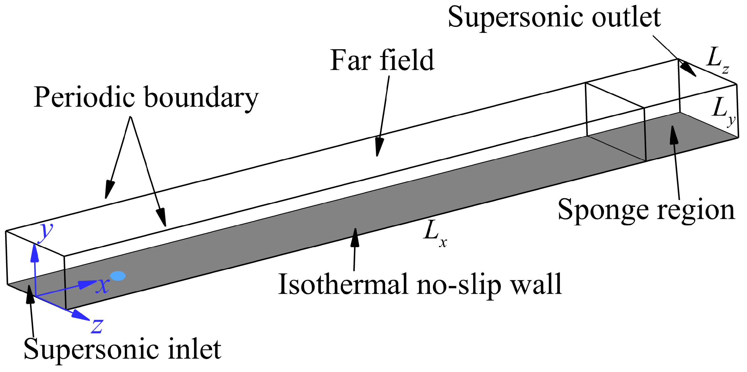
3.1. Description of Problem

The roughness configurations investigated in this study were implemented under isothermal wall conditions at temperature $T_w$.

Table 1. Freestream and wall conditions.

${\mathit{Ma}}_{\infty }$	${\mathit{Re}}_{\infty }$, m−1	${\mathit{T}}_{\infty }$, K	${\mathit{T}}_{\mathit{w}}$, K	${\mathit{\delta }}_{\mathit{r}}$, mm	${\mathit{Re}}_{\mathit{k}}$
3.5	1.08 × 107	92.55	290	0.6242	770

lists the specific inflow conditions and wall parameters. It can be seen that the freestream Mach number $M{a}_{\infty }$, Reynolds number $R{e}_{\infty }$ and static temperature $T_{\infty }$ are 3.5, $1.08$×${10}^7$ m⁻¹ and 92.55 K, respectively. The wall temperature $T_w$ is 290 K. The nominal boundary layer thickness ${\delta }_r$ and characteristic Reynolds number $R{e}_k$ at the roughness element are $0.6242$ mm and 770, respectively. A detailed description of the critical Reynolds number ($R{e}_k$) and related dimensionless parameters is provided in

Table A1. Summary of Key π-Groups in Supersonic Boundary Layer Transition Induced by Roughness Elements.

Dimensionless Parameter	Definition	Physical Significance	Role in the Investigated Problem
Mach number ($Ma$)	$Ma$ = $v/a$	Characterizes compressibility effects, governing shock formation, energy conversion (kinetic to internal) and flow separation thresholds.	In supersonic flow ($Ma$ = 3.5), compressibility dominates shock structures and shear layer stability, influencing vortex interactions.
Characteristic Reynolds number ($R{e}_k$)	$R{e}_k={\displaystyle \frac{{\rho }_k{u}_k{k}_r}{{\mu }_k}}$	Quantifies inertial-to-viscous force ratio at roughness height, determining critical instability thresholds.	The critical $R{e}_k$ = 770 triggers shear layer separation and vortex shedding, pivotal for transition onset.
Relative roughness height ($k/\delta$)	$k/\delta$	Ratio of roughness height to boundary layer thickness, defining perturbation intensity and separation scales.	Moderate $k/\delta$ = 0.64 balances disturbance strength and boundary layer adaptability, directly governing shear layer and vortex generation.
Spacing ratio ($S/W$)	$S/W$	Spanwise spacing-to-width ratio of roughness strips, modulating vortex interactions and energy transfer.	The S/W ratio magnitude affects vortex interactions and influences the variation in transition location.

of Appendix A.

The characteristic Reynolds number is defined as [38]:

$$R{e}_k={\displaystyle \frac{{\rho }_k{u}_k{k}_r}{{\mu }_k}}$$

(14)

where $R{e}_k$, ${\rho }_k$ and ${\mu }_k$ represent the Reynolds number, density and dynamic viscosity, respectively, of the fluid at the elevation corresponding to the roughness element within the unperturbed base flow. The parameter $k_r$ denotes the height of the roughness element. The shape function of the rough elements is defined as:

$$\begin{array}{c}{y}_1(x,z)=k_r\mathrm{R}\left(x\right)S\left(z\right),\\ R\left(x\right)=\left\{\begin{array}{cc}{\displaystyle \frac{1}{2}}\left[1-cos\left({\displaystyle \frac{2\pi }{x_r}}\left[x-x_s\right]\right)\right],\hfill & \left(x_s<x<x_s+x_r\right)\hfill \\ 0,\hfill & \mathrm{otherwise}\hfill \end{array}\right.\\ S\left(z\right)={\displaystyle \frac{1}{2}}\left[1-cos\left(10\pi {\displaystyle \frac{z}{L_z}}+\pi \right)\right]\end{array}$$

(15)

The geometry of the roughness element is defined by several key parameters: $k_r$, $x_r$, $x_s$ and $l_z$. In this context, $x_r$ correspond to the dimensions of the roughness element in the streamwise, respectively. Additionally, $x_s$ indicate the initial coordinates of the roughness element in the streamwise directions. For both the roughness elements and strip, the respective $k_r$ and $x_r$ parameters measure 0.4 mm and 1.8 mm. And $k_r$ represents the height of the roughness element and roughness strip, which is 0.4 mm. The centroid of the roughness element is positioned at x = 41.5 mm and z = 0 mm. Then the roughness element has dimensions of $l_x$ × $l_z$ × $k_r$ = 3.8 mm × 3.8 mm × 0.4 mm, where $l_x$ and $l_z$ represent the streamwise and spanwise extents, respectively. Furthermore, the roughness strips are characterized by dimensions of 3.8 mm × 10.8 mm × 0.4 mm, exhibiting a periodic pattern in the spanwise direction. Figure 1 offers a comprehensive depiction of the morphological features of both the roughness elements and strips on the wall surface, with the streamwise and spanwise grids illustrated at intervals of every three grid points.The roughness element and strip are demarcated by blue regions in the Figure 1. Both configurations feature refined grid clustering in the streamwise direction with uniform spacing, where the element height progressively increases with darker blue coloration. The roughness strip exhibits spanwise periodicity of 3, while maintaining identical geometric configurations to the isolated roughness elements.

The computational domain configuration is depicted in Figure 2. Supersonic flow enters the domain through the left boundary, with progressive mesh refinement applied downstream. To suppress numerical artifacts from the outflow boundary, a sponge zone is integrated at the domain’s trailing edge. The lateral boundaries of the computational domain were assigned periodic boundary conditions, while the supersonic outflow boundary was configured with a pressure-outlet condition. A non-reflective far-field boundary condition was imposed along the upper boundary of the computational domain, with the lower wall surface maintained under an isothermal no-slip condition. The inlet profile of the computational domain is set as a laminar boundary layer profile, which can be obtained by solving the following compressible laminar boundary layer similarity equations [39]:

$$\left.\begin{array}{c}{\displaystyle \frac{\mathrm{d}}{\mathrm{d}\eta }}\left({\displaystyle \frac{\rho \mu }{{\rho }_{\infty }{\mu }_{\infty }}}{\displaystyle \frac{{\mathrm{d}}^{2}f}{\mathrm{d}{\eta }^2}}\right)+f{\displaystyle \frac{{\mathrm{d}}^{2}f}{\mathrm{d}{\eta }^2}}=0\\ {\displaystyle \frac{\mathrm{d}}{\mathrm{d}\eta }}\left({\displaystyle \frac{\rho \mu }{{\rho }_{\infty }{\mu }_{\infty }}}{\displaystyle \frac{\mathrm{d}g}{\mathrm{d}\eta }}\right)+Prf{\displaystyle \frac{\mathrm{d}g}{\mathrm{d}\eta }}+Pr(\gamma -1)M_{\infty }^2{\displaystyle \frac{\rho \mu }{{\rho }_{\infty }{\mu }_{\infty }}}{\left({\displaystyle \frac{{\mathrm{d}}^{2}f}{\mathrm{d}{\eta }^2}}\right)}^2=0\end{array}\right\}$$

(16)

with

$${\displaystyle \frac{\mathrm{d}f}{\mathrm{d}\eta }}={\displaystyle \frac{u}{u_{\infty }}},g={\displaystyle \frac{T}{T_{\infty }}},\eta ={\displaystyle \frac{u_{\infty }}{\sqrt{2\xi }}}{\int }_0^y\rho \mathrm{d}y,\xi ={\int }_0^x{\rho }_{\infty }{u}_{\infty }{\mu }_{\infty }\mathrm{d}x$$

(17)

and

$$f\left(0\right)={\left.{\displaystyle \frac{\mathrm{d}f}{\mathrm{d}\eta }}\right|}_{\eta =0}=0,g\left(0\right)={\displaystyle \frac{T_w}{T_{\infty }}},\underset{\eta \to +\infty }{lim}{\displaystyle \frac{\mathrm{d}f}{\mathrm{d}\eta }}=\underset{\eta \to +\infty }{lim}g=1$$

(18)

The computational domain dimensions in this study are $L_x$ × $L_y$ × $L_z$ = 290 mm × 60 mm × 10.8 mm, with the primary computational domain spanning from x = 10 mm to x = 250 mm. The sponge zone extends along the streamwise direction from x = 250 mm to x = 300 mm, having a length of 50 mm.

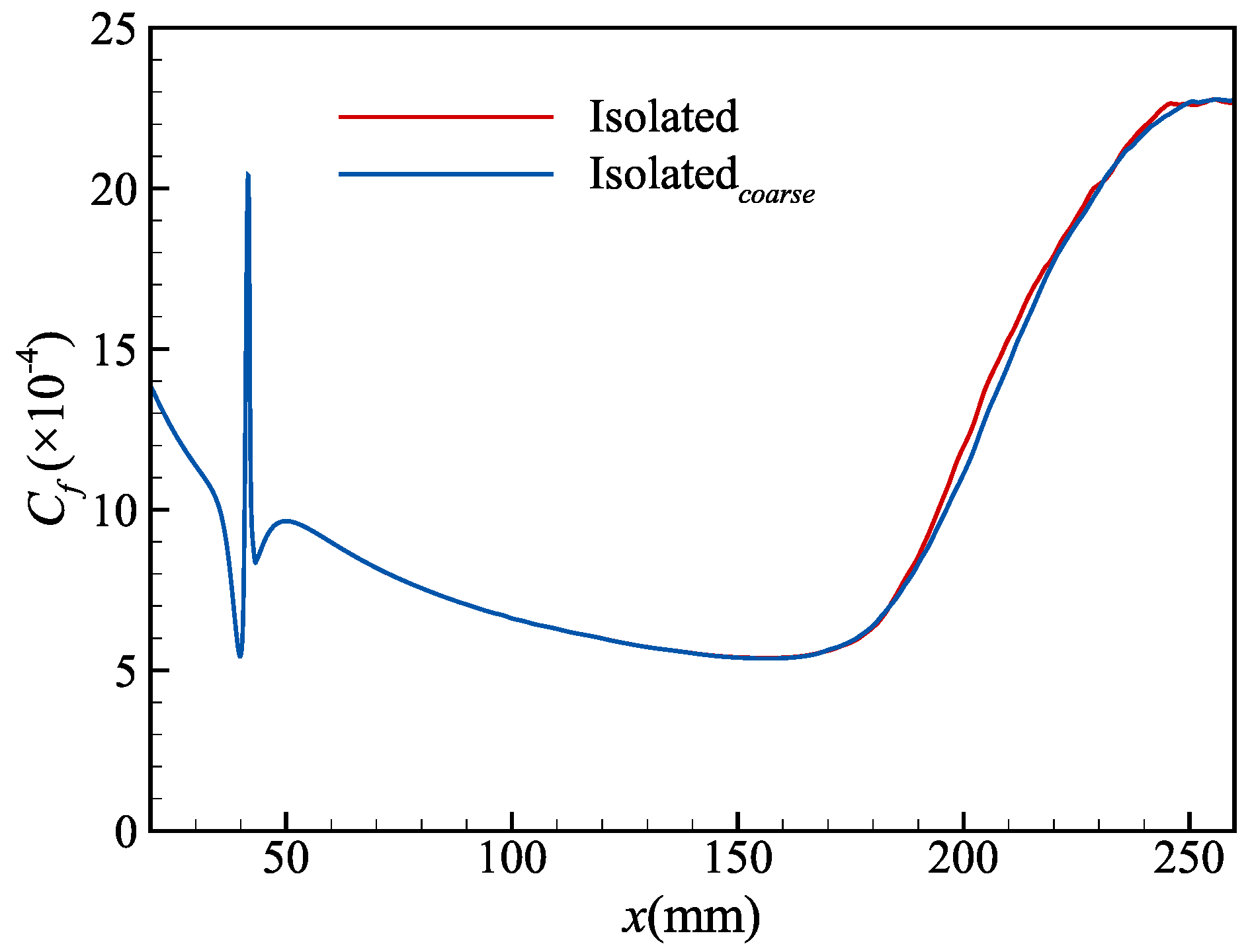
3.2. Grid Independence Study

Grid independence verification was performed to ensure computational accuracy by conducting numerical simulations on two distinct grid systems. The grid counts and resolutions are summarized in

Table 2. Details for the grid independence study.

Case	${\mathit{N}}_{\mathit{x}}\times {\mathit{N}}_{\mathit{y}}\times {\mathit{N}}_{\mathit{z}}$	$\Delta {\mathit{x}}_{\mathit{max}}^{+}\times \Delta {\mathit{y}}_{\mathit{w}}^{+}\times \Delta {\mathit{z}}_{\mathit{max}}^{+}$
Isolated	3888 × 156 × 363	5.6 × 0.85 × 2.7
Isolatedcoarse	3120 × 135 × 289	7.0 × 0.95 × 3.4

, where the baseline grid for isolated roughness element simulations comprises $N_x\times N_y\times N_z$ = 3888 × 156 × 363 with grid resolution $\Delta x_{max}^{+}\times \Delta y_w^{+}\times \Delta z_{max}^{+}$ = 5.6 × 0.85 × 2.7, denoted as Isolated. A coarser grid ($N_x\times N_y\times N_z$ = 3120 × 135 × 289, $\Delta x_{max}^{+}\times \Delta y_w^{+}\times \Delta z_{max}^{+}$ = 7.0 × 0.95 × 3.4), labeled Isolated_coarse, serves as the comparative case. Notably, identical grid parameters were implemented for both roughness elements and strips in this study, and therefore are not reiterated herein.

Figure 3 compares the time- and spanwise-averaged skin friction coefficient $C_f$ distributions. Excellent agreement is observed between both grid systems from the inlet to x = 180 mm. Within the transitional regime downstream of x = 180 mm, the $C_f$ values for Isolated_coarse are slightly underpredicted compared to Isolated, albeit with marginal discrepancy. The current grid resolution therefore proves sufficient for DNS requirements, accurately capturing the complete transition process induced by roughness elements.

4. Transition Analysis of Roughness Elements and Strips

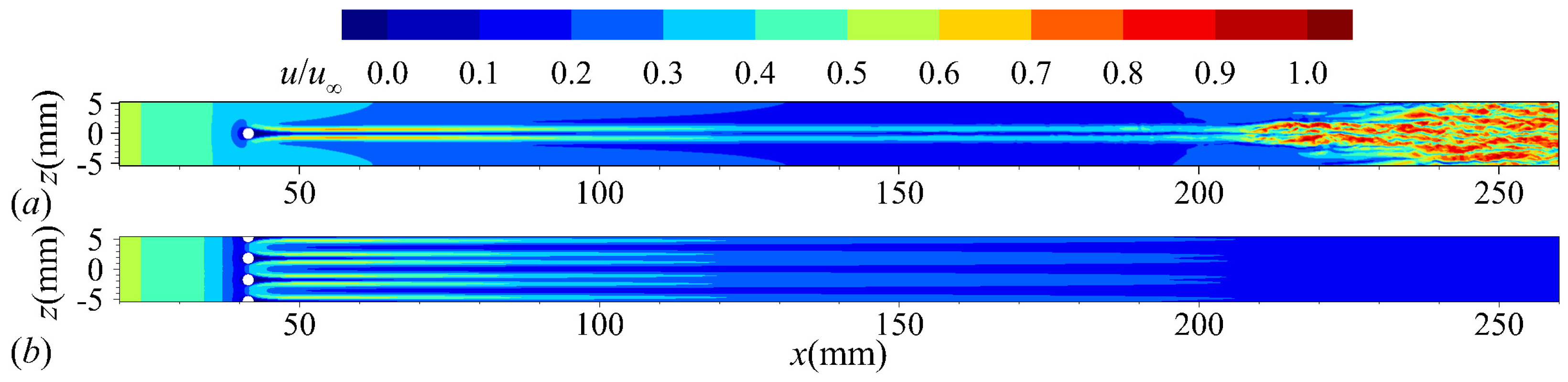
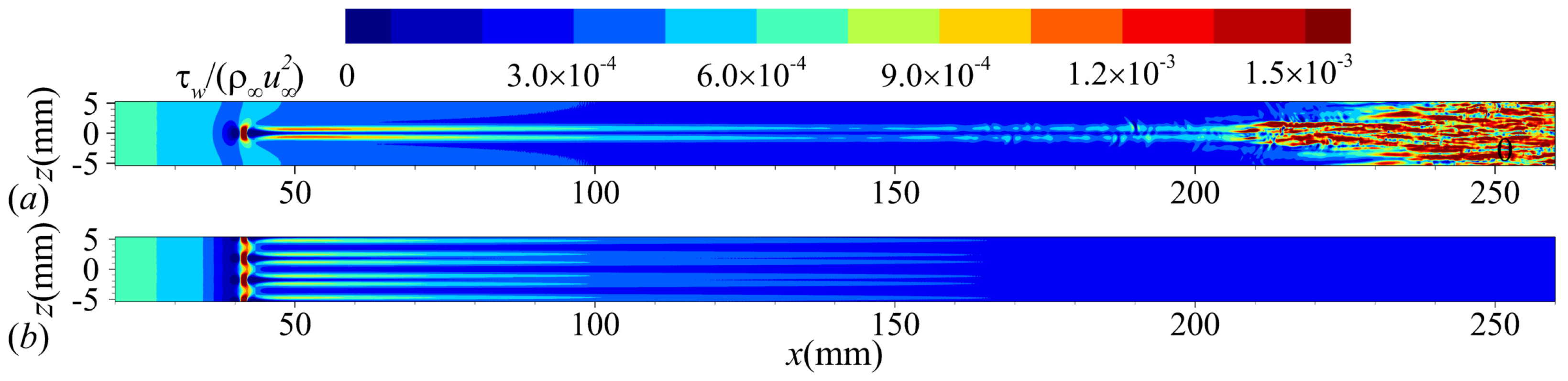
4.1. General Flow Features

This section examines the characteristic flow patterns induced by both isolated roughness elements and distributed roughness strips. Figure 4 illustrates the streamwise velocity u contours at y = 0.5$k_r$ for both configurations. For the isolated roughness case (Figure 4a), the incoming flow exhibits upstream deceleration, with two distinct high-momentum streaks emerging in the wake region. These streaks maintain coherence in the near-wake but undergo spanwise instability development further downstream. The streaks initially interact near the centerline, followed by progressive spanwise breakdown, ultimately leading to full turbulent transition across the spanwise domain. In contrast, the roughness strip configuration generates six high-momentum streaks downstream of the disturbance. These streaks exhibit gradual attenuation with downstream development, eventually dissipating without triggering turbulent transition.

Figure 5 illustrates the wall shear stress distributions on the respective surfaces under both the roughness element and roughness strip configurations. The distribution characteristics exhibit correspondence with the streamwise velocity contour patterns. As shown in Figure 5a, under the roughness element configuration, elevated wall shear stress is observed over the crest regions of individual roughness elements. Concurrently, two distinct high-shear stress streaks emerge in the wake region, demonstrating progressive streamwise attenuation. These streaks initiate interaction at approximately 210 mm in the streamwise direction, ultimately manifesting as a pronounced high-shear stress region in the downstream spanwise direction. Similarly, in the roughness strip configuration as shown in Figure 5b, localized shear stress intensification occurs at the apex of each roughness element, with inter-element regions developing streaks exhibiting streamwise-decaying intensity downstream of adjacent roughness elements. Moreover, the diminished shear stress intensity in the wake region of the roughness strip configuration compared to the roughness element configuration provides further elucidation for the velocity distribution characteristics observed in Figure 4.

Figure 6 presents the time- and spanwise-averaged flow statistics for both roughness element and strip cases. In Figure 6a, the temporally and spatially averaged skin friction coefficient $C_f$ for the isolated roughness case exhibits three distinct phases: gradual upstream attenuation due to adverse pressure gradients; abrupt amplification at the roughness station at x = 180 mm caused by flow stagnation and shear layer detachment; and progressive downstream relaxation. The sharp $C_f$ rise at x = 180 mm correlates with the onset of high-momentum streak interactions, marking the initiation of nonlinear instability mechanisms. Figure 6b quantifies the evolution of the momentum thickness Reynolds number $R{e}_{\theta }$, expressed as follows:

$$R{e}_{\theta }={\displaystyle \frac{{\rho }_{\infty }{u}_{\infty }\theta }{{\mu }_{\infty }}}$$

(19)

$$\theta ={\int }_0^{\infty }{\displaystyle \frac{\rho u}{{\rho }_{\infty }{u}_{\infty }}}\left(1-{\displaystyle \frac{u}{u_{\infty }}}\right)dy$$

(20)

Figure 6b reveals distinct evolutionary trends in the $R{e}_{\theta }$: (1) gradual growth in the upstream laminar region, (2) abrupt amplification at the roughness station and (3) accelerated growth beyond x = 180 mm, indicative of transition onset. Cross-referencing the $C_f$ and $R{e}_{\theta }$ profiles with the streamwise velocity contours at y = 0.5$k_r$ demonstrates strong quantitative agreement, validating the coupled nature of these transition indicators.

To further examine the typical flow characteristics of roughness elements and strips, Figure 7 illustrates the distribution of the wall friction coefficient $C_f$, pressure distribution and streamline patterns at cross-sections of z = 0 mm for the roughness element and z = −1.8 mm for the roughness strip. Additionally, it depicts the streamwise vortex distribution and streamline features at the cross-section of x = 60 mm.

The analysis indicates that the flow structures in both scenarios are comparable. In the upstream region, the incoming flow decelerates, resulting in a pressure increase ahead of both the roughness element and strip, with a shock wave forming at the top. The streamline patterns through the z-sections reveal a separation zone preceding both the roughness element and strip. In the wake region, distinct $C_f$ streaks are evident, with multiple pairs of streaks observed behind the roughness strip and a single pair behind the roughness element. Notably, the $C_f$ streaks behind the roughness strip are more confined. Examination of the flow characteristics at the x = 60 mm cross-section reveals typical structures such as counter-rotating vortex pairs and horseshoe vortices. Multiple vortex pairs are present behind the roughness strip, with the vortex intensity being comparatively weaker. The local shear strength for the roughness element at sections Figure 8a z = 0 mm and Figure 8b z = −1.8 mm is presented in Figure 8, and it is defined as follows:

$$u_s=\sqrt{{\left({\displaystyle \frac{\partial u}{\partial y}}\right)}^2+{\left({\displaystyle \frac{\partial u}{\partial z}}\right)}^2}$$

(21)

It is observed that the shear layer gradually detaches and evolves into a distinct separated shear layer above the roughness element’s upper surface. This phenomenon significantly enhances the likelihood of interaction with counter-rotating vortex pairs, thereby facilitating the transition from laminar to turbulent flow. From Figure 8, it can be inferred that the shear strength of the detached shear layer at the top of the roughness strip is relatively weak and diminishes at a faster rate.

To further elucidate the correlation between the detached shear layer over the roughness element and the counter-rotating vortex pairs in the wake region, Figure 9 provides an analysis of the streamwise vorticity distribution associated with both the roughness element and strip at the cross-section of x = 60 mm. In the corresponding figure, streamwise vorticity is color-coded, with thin black solid lines depicting the projection of the roughness element and strip. Examining the streamwise velocity contours, along with the thick black solid lines representing the roughness element and strip projection on this cross-section, it is evident from the streamwise vorticity plot that counter-rotating vortex pairs emerge beneath the separated shear layer over the roughness element. The airflow navigates around the roughness element, giving rise to horseshoe vortices on both sides. The vortex system associated with the roughness strip exhibits similarities to that of the roughness element; however, the roughness strip generates multiple pairs of counter-rotating and horseshoe vortices. Furthermore, the vortex strength downstream of the roughness strip is markedly lower than that observed behind the roughness element.

Considering the streamwise vorticity, mathematically defined as $w_x=\partial w/\partial y-\partial v/\partial z$, a more in-depth investigation of streamwise vortices is conducted in Figure 10 and Figure 11. These figures present spanwise and wall-normal velocity gradient contour plots at x = 60 mm for both the roughness element and roughness strip. The black solid lines in these figures outline the projected boundaries of the roughness element and roughness strip on this cross-section. The velocity gradient is observed to be more pronounced as the flow passes over the roughness element than over the roughness strip. This suggests that the spanwise and wall-normal velocity gradients are larger in the case of the roughness element, leading to stronger vortex structures in its downstream region.

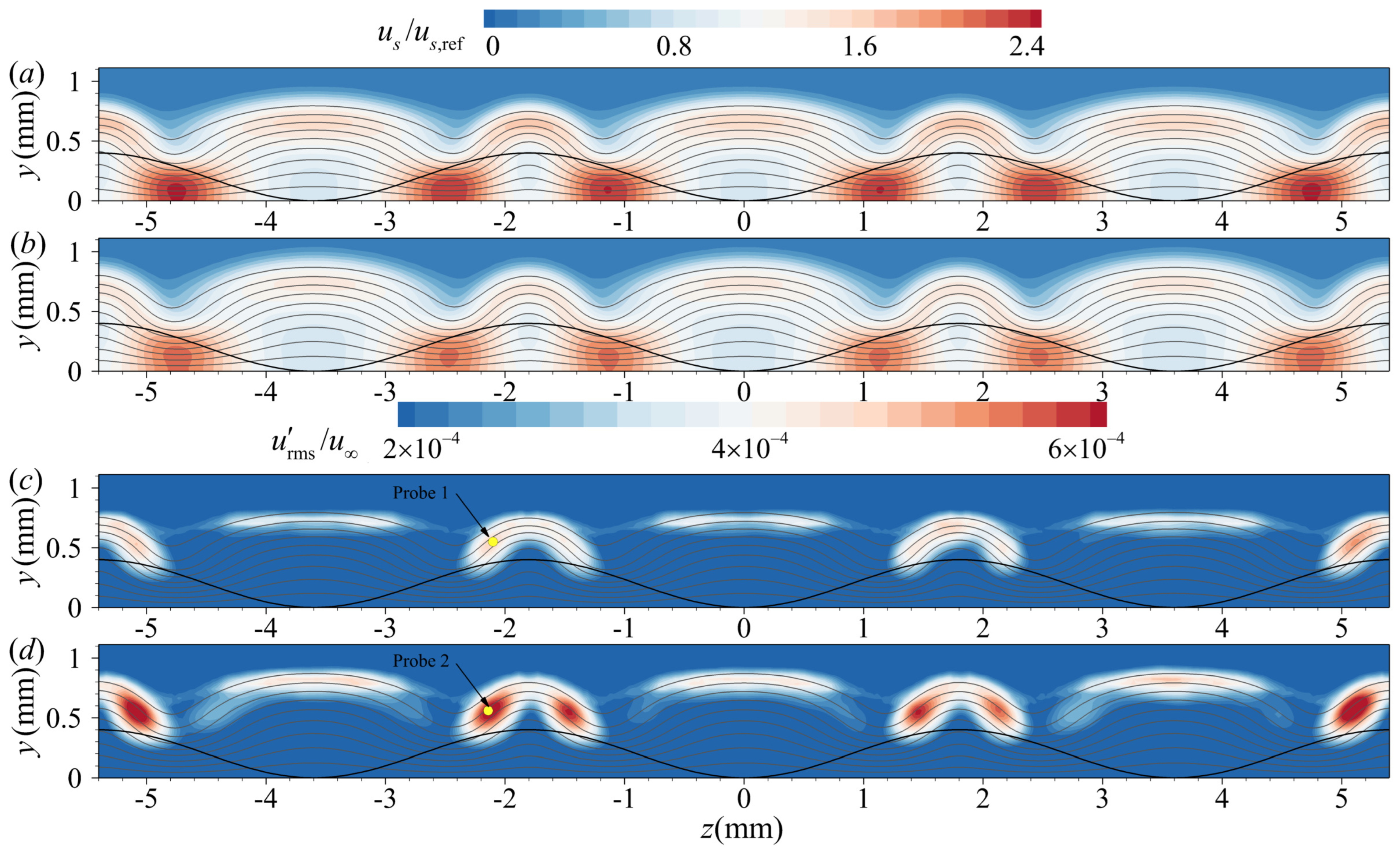
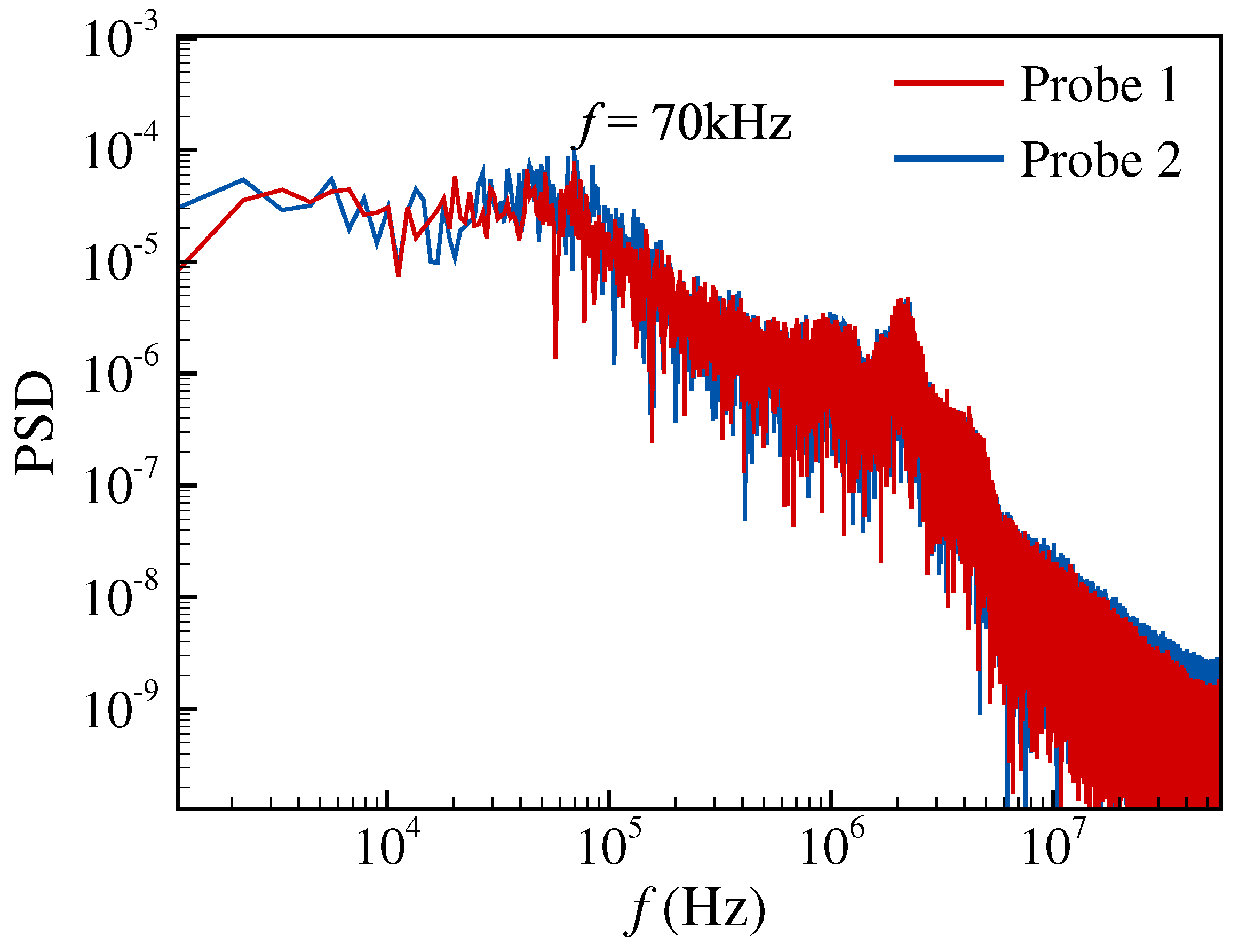
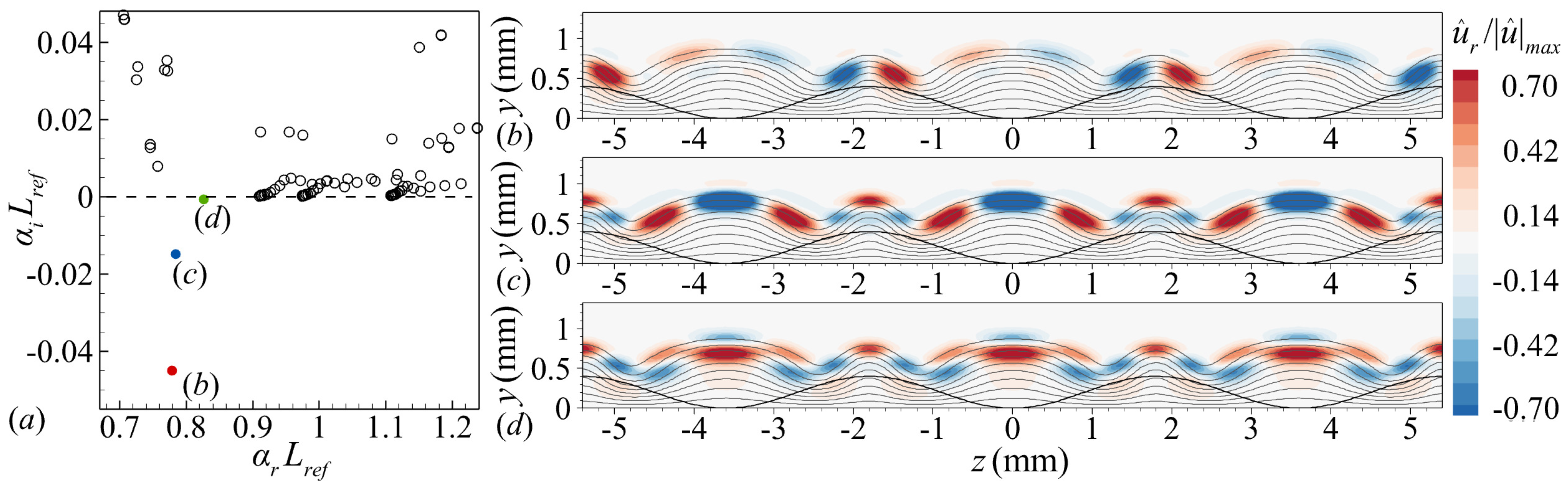
4.2. Instabilities in the Wake Region of the Roughness Element

The preceding analysis suggests that roughness elements and strips play a crucial role in promoting the transition from laminar to turbulent flow. To further investigate this phenomenon, this section focuses on the stability characteristics of the wake region behind the roughness element.

Figure 12 illustrates the shear strength and velocity fluctuation at cross-sections of x = 70 mm and x = 80 mm for the roughness element. In this figure, thin black solid lines delineate the streamwise velocity contours, while thick black solid lines highlight the projected boundaries of the roughness element and strip at these cross-sections. Figure 12a,b visualize shear strength distributions, whereas Figure 12c,d represent velocity fluctuations. Notably, Probes 2 and 4 are positioned at the upper boundary of the separated shear layer, while Probes 1 and 3 are located at the lateral root of the detached shear layer. The analysis on the same cross-section reveals that the separated shear layer at the roughness element crest exhibits higher shear strength, with both shear peak values and velocity fluctuation peaks concentrated on the z = 0 plane. However, lower-intensity fluctuations are observed at both sides of the shear layer (i.e., roughness element flanks) within the x = 80 mm cross-section. As the flow progresses further downstream, the intensity of the upper shear layer gradually diminishes, whereas velocity fluctuations increase.

To integrate these findings, power spectral density (PSD) analysis was performed on four probes (Probe 1–4) at the two cross-sections, with the results presented in Figure 13. The figure reveals two distinct amplitude peaks on both cross-sections, where all four measurement probes exhibit maximum energy at f = 138 kHz, with identical peak frequencies across the probes. This frequency synchronization indicates dominant control over the development of both the shear layer and counter-rotating vortex pairs. The consistent peak frequencies between cross-sections demonstrate that all four probes reside within the same vortex system. Additionally, the secondary peaks’ lower amplitudes render their influence on the flow field negligible; therefore, subsequent analyses exclude these components.

Furthermore, a BiGlobal stability analysis was conducted at the cross-section x = 80 mm for f = 138 kHz, with the results illustrated in Figure 14. This figure showcases streamwise velocity contours, where thin black solid lines indicate the streamwise velocity and thick black solid lines mark the projected outline of the roughness element. Figure 14a displays a portion of the eigenvalue spectrum, identifying five distinct unstable modes. Figure 14b–f display the real components of the streamwise velocity eigenfunctions (${\widehat{u}}_r$) corresponding to these modes. In Figure 14, mode b exhibits a higher growth rate, with its modal distribution demonstrating symmetry about the z = 0 mm cross-section. By combining the streamwise velocity contours and modal distribution, it can be observed that the peak values of mode bare predominantly concentrated within the separated shear layer at the crest of the roughness element. Meanwhile, in Figure 14c, the mode has the second-largest growth rate and its distribution is antisymmetric about the z = 0 mm cross-section, while weaker distributions are observed within the shear layers on both sides of the roughness element. Based on these distribution features, modes b and c are, respectively, designated as symmetric and antisymmetric modes. Modes d–f in Figure 14 display antisymmetric, symmetric and antisymmetric distribution patterns correspondingly. However, these three modes exhibit relatively low growth rates and more dispersed modal distributions, resulting in negligible influence on wake disturbances. Based on the comprehensive analysis above, it can be observed that mode b, which has dominant growth characteristics, has its modal distribution peaks concentrated within the separated shear layer region originating from the roughness element crest. Consequently, the BiGlobal stability analysis further substantiates that the primary instability in the wake originates from the interplay between the detached shear layer and the counter-rotating vortex pairs downstream of the roughness element, with the symmetric mode exerting a dominant influence. This finding precisely corresponds with the results shown in Figure 12.

4.3. Instabilities in the Wake Region of Roughness Strip

This section investigates the stability characteristics of roughness strip wakes to elucidate fundamental differences between isolated roughness elements and distributed strips in triggering boundary layer transition.

Figure 15 illustrates the spatial distributions of shear strength magnitude and velocity perturbation amplitudes at two streamwise stations (x = 70 mm and x = 80 mm) downstream of the roughness strip. In this figure, thin black solid lines denote streamwise velocity contours, while thick black solid lines outline the projections of the roughness elements and roughness strips onto the cross-sections. Figure 15a,b depict shear strength variations, while Figure 15c,d illustrate velocity fluctuation distributions. Probes 1 and 2 are positioned at the lateral root of the separated shear layer. A cross-sectional analysis reveals that the shear strength at the upper boundary of the separated shear layer over the roughness elements is on par with that between adjacent roughness elements, with peak distributions exhibiting significant dispersion. Velocity fluctuation peaks are observed on both sides of the shear layer above the roughness elements, with substantial fluctuations spanning across neighboring roughness structures. In the streamwise direction, the shear strength of the separated shear layer over the roughness elements and between adjacent roughness elements diminishes progressively, whereas velocity fluctuations intensify. A comparative analysis between Figure 12 and Figure 15 reveals that the velocity fluctuation intensity downstream of the roughness strip is one order of magnitude lower than that downstream of the roughness element. Combined with the streamwise vorticity contours in Figure 9, this observation indicates that the reduced inter-element spacing within the roughness strip creates an aerodynamic shielding effect analogous to a “barrier”, which diminishes vortex strength downstream. Furthermore, vortex-vortex interactions suppress sustained vortex growth in the wake region.

Expanding upon these findings, PSD analyses of Probes 1 and 2 at both cross-sections are conducted, with the results presented in Figure 16. The PSD analysis reveals that the energy of Probes 1 and 2 (located at the lateral root of the separated shear layer) attains its peak at 70 kHz. This phenomenon is attributed to the probes being embedded within counter-rotating vortex pairs. The figure also reveals the presence of a secondary peak, whose intensity is one order of magnitude lower than the primary peak. Given its negligible impact on wake disturbances, this secondary component will not be subjected to further analysis in subsequent discussions.

Subsequently, BiGlobal stability analysis is performed at x = 80 mm for the dominant frequency f = 70 kHz, with the results depicted in Figure 17. Thin black solid lines represent streamwise velocity contours, and thick black solid lines demarcate the roughness strip projection. Figure 17a displays three unstable modes b, c and d at the specified frequency, with their modal distributions illustrated in the right panel. Among these, the antisymmetric mode in Figure 17b exhibits the most pronounced growth rate, with its modal peaks concentrated within the separated shear layer above the roughness elements. Figure 17c corresponds to a symmetric mode, with its modal distribution predominantly concentrated within the shear layer between two adjacent roughness elements. The modal intensity in this region exceeds that observed in the shear layer at the roughness element crests. Figure 17d exhibits a symmetric mode characterized by spanwise-uniform distribution, manifesting a vertically stratified structure within the upper shear layer region. The modal characteristics observed in Figure 17 indicate that the dominant instability is primarily associated with the antisymmetric mode illustrated in Figure 17b. So generally, BiGlobal stability analysis of the roughness strip wake reveals that the primary instability mechanism originates from the coupling between the shear layer separated from the roughness element crests and the downstream counter-rotating vortex pairs. However, unlike the isolated roughness element case, the antisymmetric mode dominates wake development in the roughness strip configuration.

5. Conclusions

This study examines the mechanisms by which roughness elements and strips with distinct geometries influence the transition from laminar to turbulent flow over an isothermal no-slip flat plate under supersonic flow conditions. To capture the complete transition process, DNS were conducted. Subsequently, the key flow characteristics were analyzed, followed by an in-depth investigation of the instability mechanisms associated with wake vortices using BiGlobal stability analysis.

The DNS results indicate that roughness elements effectively trigger laminar-to-turbulent transition within the boundary layer. In contrast, roughness strips do not directly cause transition, though they still generate unsteady flow structures in their wake. Visualization of the upper shear layers and wake vortices reveals that the dominant sources of instability arise from the top shear layer and counter-rotating vortex pairs in the wake. For roughness elements, a single pair of counter-rotating vortices interact with the separated shear layer at the top. Conversely, in the case of roughness strips, multiple counter-rotating vortex pairs interact with not only the top separated shear layer but also the shear layer between adjacent roughness elements and the horseshoe vortices. The vortical structures behind roughness strips exhibit comparatively weaker intensity. Analysis of the streamwise shear strength and velocity fluctuations shows that, for roughness elements, peak values are predominantly concentrated in the upper region of the separated shear layer. On the other hand, roughness strips exhibit a broader distribution of shear strength peaks, while velocity fluctuation peaks appear on both sides of the top separated shear layer and within the shear layer between adjacent roughness elements. Furthermore, shear strength and velocity fluctuation peaks are primarily distributed along both sides of the roughness element crests. BiGlobal stability analysis identifies two primary unstable modes in the wake: symmetric and antisymmetric. The results indicate that, for roughness elements, the symmetric mode exhibits a higher growth rate, whereas, for roughness strips, the antisymmetric mode tends to dominate with a larger growth rate.

The influence of roughness element height on boundary layer transition has been investigated through flow visualization and DNS by Han et al. [40] and Kosuke et al. [41], respectively. Consequently, further research and experimental investigations are required to systematically examine the effects of roughness element shape parameters and roughness strips spacing on transition mechanisms.

Currently, it should be noted that DNS imposes extremely high requirements on grid quantity and time step size, requiring substantial computational costs (As shown in Appendix B the computational resources and time used in this study). Meanwhile, BiGlobal neglects the influence of nonlinear disturbances, which may underestimate the threshold of actual flow and fails to address stability issues in fully three-dimensional non-uniform flows. Therefore, it is necessary to enhance their practicality and efficiency through hybrid methods, multi-scale coupling and the development of high-performance computing infrastructure.

References

1. Bernardini, M.; Pirozzoli, S.; Orlandi, P.; Lele, S.K. Parameterization of Boundary-Layer Transition Induced by Isolated Roughness Elements. AIAA J. 2014, 52, 2261–22619. [Google Scholar] [CrossRef]
2. Berry, S.A.; Horvath, T.J. Discrete-Roughness Transition for Hypersonic Flight Vehicles. J. Spacecr. Rocket. 2008, 45, 16–27. [Google Scholar] [CrossRef]
3. Choudhari, M.; Norris, A.; Li, F.; Chang, C.-L.; Edwards, J. Wake Instabilities behind Discrete Roughness Elements in High Speed Boundary Layers. In Proceedings of the 51st AIAA Aerospace Sciences Meeting Including the New Horizons Forum and Aerospace Exposition, Grapevine, TX, USA, 7–10 January 2013; p. 81. [Google Scholar]
4. Lu, Y.; Zeng, F.; Liu, H.; Liu, Z.; Yan, C. Direct numerical simulation of roughness-induced transition controlled by two-dimensional wall blowing. J. Fluid Mech. 2021, 28, 920. [Google Scholar] [CrossRef]
5. Fu, S.; Wang, L. RANS modeling of high-speed aerodynamic flow transition with consideration of stability theory. Prog. Aerosp. Sci. 2013, 58, 36–59. [Google Scholar] [CrossRef]
6. Lu, Y.; Liu, Z.; Zhou, T.; Yan, C. Stability analysis of roughness-disturbed boundary layer controlled by wall-blowing. Phys. Fluids 2022, 34, 104–114. [Google Scholar] [CrossRef]
7. Van den Eynde, J.P.; Sandham, N.D. Numerical Simulations of Transition due to Isolated Roughness Elements at Mach 6. AIAA J. 2016, 54, 53–65. [Google Scholar] [CrossRef]
8. Kneer, S.; Guo, Z.; Kloker, M.J. Control of laminar breakdown in a supersonic boundary layer employing streaks. J. Fluid Mech. 2022, A53, 9–32. [Google Scholar] [CrossRef]
9. De Tullio, N.; Paredes, P.; Sandham, N.D.; Theofilis, V. Laminar–turbulent transition induced by a discrete roughness element in a supersonic boundary layer. J. Fluid Mech. 2013, 735, 13–46. [Google Scholar] [CrossRef]
10. Balakumar, P.; Kegerise, M. Roughness-Induced Transition in a Supersonic Boundary Layer. AIAA J. 2016, 54, 22–37. [Google Scholar] [CrossRef]
11. Choudhari, M.; Li, F.; Chang, C.-L.; Edwards, J.; Kegerise, M.; King, R. LLaminar-Turbulent Transition behind Discrete Roughness Elements in a High-Speed Boundary Layer. In Proceedings of the 48th AIAA Aerospace Sciences Meeting Including the New Horizons Forum and Aerospace Exposition, Orlando, FL, USA, 4–7 January 2010; p. 1575. [Google Scholar]
12. Semper, M.T.; Bowersox, R.D.W. Tripping of a Hypersonic Low-Reynolds-Number Boundary Layer. AIAA J. 2017, 55, 8–17. [Google Scholar] [CrossRef]
13. Bartkowicz, M.; Subbareddy, P.; Candler, G. Numerical Simulations of Roughness Induced Instability in the Purdue Mach 6 Wind Tunnel. In Proceedings of the 40th Fluid Dynamics Conference and Exhibit, Chicago, IL, USA, 28 June–1 July 2010; p. 4723. [Google Scholar]
14. Casper, K.; Wheaton, B.; Johnson, H.; Schneider, S. Effect of Freestream Noise on Roughness-Induced Transition at Mach 6. In Proceedings of the 38th Fluid Dynamics Conference and Exhibit, Seattle, WA, USA, 23–26 June 2008; p. 4291. [Google Scholar]
15. Wang, L.; Yang, R.; Zhou, Y.; Zhao, Y. Roughness effect of an acoustic metasurface on supersonic boundary layer transition. Appl. Phys. Lett. 2023, 123, 141701. [Google Scholar] [CrossRef]
16. Kurz, H.B.E.; Kloker, M.J. Mechanisms of flow tripping by discrete roughness elements in a swept-wing boundary layer. J. Fluid Mech. 2016, 796, 58–94. [Google Scholar] [CrossRef]
17. Bernardini, M.; Pirozzoli, S.; Orlandi, P. Compressibility effects on roughness-induced boundary layer transition. Int. J. Heat Fluid Flow 2012, 35, 45–51. [Google Scholar] [CrossRef]
18. Subbareddy, P.K.; Bartkowicz, M.D.; Candler, G.V. Direct numerical simulation of high-speed transition due to an isolated roughness element. J. Fluid Mech. 2014, 748, 48–78. [Google Scholar] [CrossRef]
19. De Tullio, N.; Sandham, N.D. Influence of boundary-layer disturbances on the instability of a roughness wake in a high-speed boundary layer. J. Fluid Mech. 2015, 763, 36–65. [Google Scholar] [CrossRef]
20. Shrestha, P.; Candler, G.V. Direct numerical simulation of high-speed transition due to roughness elements. J. Fluid Mech. 2019, 868, 62–88. [Google Scholar] [CrossRef]
21. Liu, Z.; Lu, Y.; Liang, J.; Huang, H. Roughness-Induced Transition in Supersonic Boundary Layers with Wall Heating and Cooling Effects. AIAA J. 2024, 62, 58–75. [Google Scholar] [CrossRef]
22. Whitehead, A.H. Flow-Field and Drag Characteristics of Several Boundary-Layer Tripping Elements in Hypersonic Flow; NTRS: Chicago, IL, USA, 1969. [Google Scholar]
23. Shrestha, P.; Candler, G.V. Direct Numerical Simulation of Trip Induced Transition. In Proceedings of the 46th AIAA Fluid Dynamics Conference, Washington, DC, USA, 13–17 June 2016; p. 4380. [Google Scholar]
24. Shrestha, P.; Nichols, J.W.; Jovanovic, M.R.; Candler, G.V. Study of Trip-Induced Hypersonic Boundary Layer Transition. In Proceedings of the 47th AIAA Fluid Dynamics Conference, Denver, CO, USA, 5–9 June 2017; p. 4513. [Google Scholar]
25. Schneider, S.P. Effects of Roughness on Hypersonic Boundary-Layer Transition. J. Spacecr. Rocket. 2008, 45, 193–208. [Google Scholar] [CrossRef]
26. De Baets, G.; Szabó, A.; Nagy, P.T.; Paál, G.; Vanierschot, M. Vortex Characterization and Parametric Study of Miniature Vortex Generators and Their Near-Field Boundary Layer Effects. Appl. Sci. 2024, 14, 6966. [Google Scholar] [CrossRef]
27. Huang, H.; Liu, Z.; Liu, M.; Tan, H. Direct numerical simulation of distributed roughness induced transition in a supersonic boundary layer. Phys. Fluids 2024, 36, 124115. [Google Scholar] [CrossRef]
28. Liu, H.; Peng, K.; Zhao, Y.; Yu, Q.; Kong, Z.; Chen, J. Direct numerical simulation of supersonic boundary layer transition induced by gap-type roughness. Adv. Aerodyn. 2024, 6, 16. [Google Scholar] [CrossRef]
29. Liu, Z.; Huang, H.; Tan, H.; Liu, M. Control of Roughness-Induced Transition in Supersonic Flows by Local Wall Heating Strips. J. Fluid Mech. 2024, 999, A16. [Google Scholar] [CrossRef]
30. Li, X.; Fu, D.; Ma, Y. Direct Numerical Simulation of Hypersonic Boundary Layer Transition over a Blunt Cone. AIAA J. 2008, 46, 899–913. [Google Scholar] [CrossRef]
31. Jiang, G.; Shu, C. Efficient Implementation of Weighted ENO Schemes. J. Comput. Phys. 1996, 126, 2–28. [Google Scholar] [CrossRef]
32. Martín, M.P.; Taylor, E.M.; Wu, M.; Weirs, V.G. A bandwidth-optimized WENO scheme for the effective direct numerical simulation of compressible turbulence. J. Comput. Phys. 2006, 220, 70–89. [Google Scholar] [CrossRef]
33. Steger, J.L.; Warming, R.F. Flux vector splitting of the inviscid gasdynamic equations with application to finite-difference methods. J. Comput. Phys. 1981, 40, 63–93. [Google Scholar] [CrossRef]
34. Zhang, W.; Samtaney, R. BiGlobal linear stability analysis on low-Re flow past an airfoil at high angle of attack. Phys. Fluids 2016, 28, 44–105. [Google Scholar] [CrossRef]
35. Sun, Y.; Taira, K.; Cattafesta, L.N.; Ukeiley, L.S. Biglobal instabilities of compressible open-cavity flows. J. Fluid Mech. 2017, 826, 270–301. [Google Scholar] [CrossRef]
36. Fernández-Gámiz, U.; Marika, V.C.; Réthoré, P.-E.; Sørensen, N.N.; Egusquiza, E. Testing of self-similarity and helical symmetry in vortex generator flow simulations. Wind. Energy 2016, 19, 43–52. [Google Scholar] [CrossRef]
37. Fassbender, H.; Kressner, D. Structured Eigenvalue Problems. Gamm-Mitteilungen 2006, 29, 297–318. [Google Scholar] [CrossRef]
38. Redford, J.A.; Sandham, N.D.; Roberts, G.T. Compressibility Effects on Boundary-Layer Transition Induced by an Isolated Roughness Element. AIAA J. 2010, 48, 18–30. [Google Scholar] [CrossRef]
39. White, F.M. Viscous Fluid Flow, 3rd ed.; McGraw-Hill: New York, NY, USA, 2006. [Google Scholar]
40. Han, J.; He, L.; Xu, X.; Wu, Z. Experimental Investigation of a Roughness Element Wake on a Hypersonic Flat Plate. Aerospace 2022, 9, 574. [Google Scholar] [CrossRef]
41. Nakagawa, K.; Takahiro, T.; Takahiro, I. DNS Study on Turbulent Transition Induced by an Interaction between Freestream Turbulence and Cylindrical Roughness in Swept Flat-Plate Boundary Layer. Aerospace 2023, 10, 128. [Google Scholar] [CrossRef]
Figure 1. Shape characteristics of the (a) roughness element and (b) roughness strip on the wall surface.
Aerospace 12 00242 g001
Figure 2. Computational domain setup.
Aerospace 12 00242 g002
Figure 3. Results of grid independence study.
Aerospace 12 00242 g003
Figure 4. Instantaneous streamwise velocity at y = 0.5 k r for (a) the roughness element and (b) the roughness strip.
Aerospace 12 00242 g004
Figure 5. Wall shear stress distribution of (a) the roughness elements and (b) the roughness strip.
Aerospace 12 00242 g005
Figure 6. Time- and spanwise-averaged flow results for the roughness element and strip: (a) wall friction coefficient C f ; (b) momentum thickness Reynolds number R e θ .
Aerospace 12 00242 g006
Figure 7. Flow characteristics around (a) the roughness element and (b) the roughness strip.
Aerospace 12 00242 g007
Figure 8. Local shear strength of (a) the roughness element at z = 0 mm and (b) the roughness strip at z = −1.8 mm.
Aerospace 12 00242 g008
Figure 9. Streamwise vorticity of (a) the roughness element and (b) the roughness strip at the cross-section of x = 60 mm.
Aerospace 12 00242 g009
Figure 10. Spanwise velocity gradient of (a) the roughness element and (b) the roughness strip at the cross-section of x = 60 mm.
Aerospace 12 00242 g010
Figure 11. Wall-normal velocity gradient of (a) the roughness strip and (b) the roughness strip at the cross-section of x = 60 mm.
Aerospace 12 00242 g011
Figure 12. Shear strength (a,b) and velocity fluctuation (c,d) of the roughness element at (a,c) x = 70 mm and (b,d) x = 80 mm.
Aerospace 12 00242 g012
Figure 13. PSD results of streamwise velocity fluctuation of roughness element at (a) probe 1 and probe 3 and (b) probe 2 and probe 4.
Aerospace 12 00242 g013
Figure 14. BiGlobal analysis results of (a) eigenvalue spectrum and (bf) real part of the streamwise velocity shape functions for roughness element. The results are obtained for f = 138 kHz at x = 80 mm. The thin black solid lines in (bf) are streamwise velocity isolines, and the thick black solid lines in (bf) represent the the projected outline of the roughness element.
Aerospace 12 00242 g014
Figure 15. Shear strength (a,b) and velocity fluctuation (c,d) of the roughness strip at (a,c) x = 70 mm and (b,d) x = 80 mm.
Aerospace 12 00242 g015
Figure 16. PSD results of streamwise velocity fluctuation of roughness strip at (red) probe 1 and (blue) probe 2.
Aerospace 12 00242 g016
Figure 17. BiGlobal analysis results of (a) eigenvalue spectrum and (bd) real part of the streamwise velocity shape functions for roughness strip. The results are obtained for f = 70 kHz at x = 80 mm. The thin black solid lines in (bd) are streamwise velocity isolines, and the thick black solid lines in (bd) represent the the projected outline of the roughness strip.
Aerospace 12 00242 g017