Research on the Dynamic Modeling of Rigid–Flexible Composite Spacecraft Under Fixed Constraints Based on the ANCF

Abstract

Dynamically modeling the flexible characteristics of large-scale jointed composite spacecraft is challenging. In this study, a dynamic modeling method for rigid–flexible composite spacecraft is proposed based on the absolute nodal coordinate formulation (ANCF). First, the spacecraft in the jointed composite is simplified as a rigid body, and the docking mechanisms between spacecraft are approximated using the fully parameterized beam model. Next, regarding the constraints between the beam and the rigid body, the beam’s absolute nodal coordinates are converted into rigid body coordinates. This allows the dynamic equations to be simplified using independent coordinates, reducing the model dimension. Finally, system damping is increased through the mean stress noise reduction method, which suppresses high-frequency components in the dynamic model and further reduces the rigidity of the dynamic equations for the composite body. This modeling method decreases the complexity of the composite body dynamics and avoids the difficulty of solving algebraic–differential equations exhibited by Lagrange multiplier methods, facilitating numerical simulations. The proposed method is applicable to both tree and mesh topologies. MATLAB simulations demonstrate that the proposed dynamic model alleviates the dimensionality disaster caused by conventional algorithms, significantly reducing computation time. The simulation results are consistent with ADAMS. The proposed model exhibits displacement errors less than 1 mm, highlighting its efficiency and accuracy.

1. Introduction

Composite spacecraft serve as a crucial means for surpassing the limitations of single launches and constructing large-scale space structures, such as space solar power stations and large-aperture antennas. Consequently, they have become a prominent research focus in the aerospace field [1]. Composite spacecraft exhibit complex topological structures and coupling between rigid and flexible components, making accurately modeling their dynamics and achieving efficient model solutions challenging [2].

In the field of flexible body dynamic modeling, conventional methods primarily include the floating coordinate method, incremental finite element method, and absolute nodal coordinate formulation (ANCF) [3]. The floating coordinate method has been widely applied in various multibody dynamics commercial software, like ADAMS-2019; it is specifically suitable for dynamic modeling and analysis of multibody systems with small deformations, small rotations, or low rotational motion [4]. Composite spacecraft belong to drifting-based multibody systems, where their attitude generally requires stability in a specific direction. As a result, spacecraft often undergo spinning at a certain angular velocity in the inertial reference frame. Considering the demands of attitude maneuvering and on-orbit operations, composite spacecraft typically fail to meet the floating coordinate method requirements of small rotations or low rotational speeds, making this method inapplicable [5]. On the other hand, the incremental finite element method cannot accurately describe the rigid body motion of systems undergoing large rotations, so it is also unsuitable for composite spacecraft with orbital motion characteristics.

Shabana [6] proposed the ANCF, which assumes the relaxation of rigid cross-sections in flexible bodies. It precisely describes the rigid displacements and deformations of beam elements through the position vector coordinates and gradient vector coordinates at the nodes in the absolute coordinate system. This formulation cleverly integrates both aspects into a single displacement field, and it thereby is able to describe complex geometric configurations. The dynamic models established based on the ANCF have constant mass matrices, and the system equations do not include centrifugal force or Coriolis force terms, reducing the computational complexity to some extent [7]. ANCF-based dynamic models of rods, beams, plates, and other structures have found wide applications and research in areas such as tethered satellites [8], complex robots [9], and space deployment mechanisms [10].

The finite element method is the most widely used approach in the field of rigid–flexible coupling multibody dynamics. Its core idea is to “divide and conquer” [11] by assembling simplified elements according to their topological structure, which mathematically involves decomposing and assembling the element mass matrix, damping matrix, and stiffness matrix [12]. Yu [13] proposed a direct assembly method for rigid body and flexible body position constraints, reducing the system dimension and improving computational efficiency. Hu [14] addressed the violation problem in the dynamic equations of multiflexible body systems by introducing a recursive absolute nodal coordinate algorithm that solves the system state incrementally for each element, significantly reducing computational complexity. Kim [15] proposed an efficient method for computing elastic forces by approximating them with a third-degree polynomial in displacement.

However, the rigid–flexible coupling dynamics of composite spacecraft ultimately result in a set of second-order nonlinear differential equations. Due to the coupling of rigid and flexible elements, these differential equations typically exhibit strong stiffness, with Lipschitz constants reaching magnitudes of 106 or higher. Consequently, a challenge arises in rigid–flexible coupling dynamics: as the stiffness of a flexible body increases, i.e., the elastic modulus or shear modulus becomes larger, the motion of the object tends to approach simple rigid body motion. However, solving the dynamic differential equation system only becomes more difficult [16]. In engineering analysis, employing stiff differential equation solvers is common; otherwise, obtaining numerical solutions within a reasonable period becomes challenging. Stiff differential equation solvers can be divided into two categories. The first category addresses first-order differential equations and includes methods such as the backward differentiation formula (BDF) [17], implicit Runge–Kutta methods [18], and Rosenbrock methods [19]. The second category addresses second-order differential equations and includes methods such as the Newmark method [20], Wilson-θ method [21], HHT method [22], and generalized-α method. These methods all employ numerical damping to remove high-frequency components from the system, ensuring that the integration step does not accumulate errors due to amplification when the step length is far greater than the smallest vibration period. Qi [23] and others proposed a noise reduction dynamic model for multiflexible body systems that increases damping and suppresses excessively high frequencies using the mean stress method, effectively reducing system stiffness and significantly improving the solution efficiency. Zhang [24] applied this method to ANCF-based beam elements and verified the feasibility of the noise reduction dynamic model. However, the noise reduction dynamic model has yet to be applied and validated in the context of rigid–flexible coupling dynamics.

Given the large number of modules in composite spacecraft and their strong dynamic equations, assembling rigid–flexible elements and efficiently solving the dynamic equations are critical issues that must be addressed. Considering that the individual dimensions of spacecraft within the composite are much smaller than the overall size and are more rigid, it is necessary to simplify dynamic modeling by treating the rigid docking mechanisms as flexible beams as possible. This simplification of the model helps reduce computational complexity and facilitates the analysis of stress, strain, and vibration characteristics at the connection points.

In this study, a direct assembly method is utilized to couple rigid and flexible elements, effectively addressing the complex position and orientation constraints between rigid units. The independent coordinates are obtained by exploiting the geometric relationship between the units, resulting in a simplified dynamic model of the rigid–flexible coupling system. To undertake the challenge of solving the dynamic equations for high-degree-of-freedom systems, a noise reduction model that can filter out high-frequency components is employed in flexible element modeling, thereby enhancing computational efficiency.

In this study, the dynamic response characteristics of composite spacecraft under orbital dynamics environments are investigated. Specifically, the vibration response characteristics of the composite spacecraft under the influence of the gravity gradient are examined. The findings provide valuable insights for spacecraft orbit design and vibration suppression.

2. Rigid–Flexible Coupling Dynamic Modeling Based on the ANCF

In a composite spacecraft, individual spacecraft are interconnected through docking mechanisms. In this paper, due to the high tiling efficiency and structural stability of hexagons, each spacecraft is simplified as a rigid hexagonal prism module, with the rigid bodies connected to each other through docking mechanisms. In contrast to rigid modules, docking mechanisms can be considered flexible beams due to their mechanical clearances and large spans. Therefore, the composite spacecraft inherently forms a network-like topology of a rigid–flexible coupling multibody system, as shown in Figure 1. When the spacecraft undergoes attitude or orbital maneuvers in space, it exhibits vibration characteristics distinct from those of a pure rigid body due to spatial disturbances and its own dynamic driving. These vibrations can impact the attitude control of the composite spacecraft.

2.1. Dynamic Modeling of Noise Reduction in Beam Elements Based on ANCF

The response of a rigid–flexible coupled multibody system is primarily influenced by low-frequency modes, with the contribution of high-frequency modes being negligible. Moreover, structural damping rapidly attenuates high-frequency responses, and the finite element discretization inherently provides a poor approximation for high-frequency modes. Therefore, achieving high precision in computing high-frequency responses during the solution process of the system’s dynamic equations is neither realistic nor necessary. Consequently, in this section, the high-frequency components induced by elastic forces in the system are treated as noise and suppressed through filtering in the modeling process.

The flexible body in the system is represented using the fully parameterized beam model based on the ANCF, as shown in Figure 1. Here, $O_i-X_i{Y}_i{Z}_i$ is the inertial reference coordinate system, $r_i$ and $r_j$ are the absolute position coordinates of nodes $i$ and $j$, and $r_{i,\mathrm{\alpha }}\left(\mathrm{\alpha }=x,y,z\right)$ and $r_{j,\mathrm{\alpha }}\left(\mathrm{\alpha }=x,y,z\right)$ are the gradient vectors of nodes $i$ and $j$. The position vector of any point on the beam at time in the inertial frame can be represented as

$$r\left(x_b,t\right)=S\left(x_b\right)e\left(t\right),$$

(1)

where $e=\left[\begin{array}{cccccccc}{r}_i& r_{i,x}& r_{i,y}& r_{i,z}& r_j& r_{j,x}& r_{j,y}& r_{j,z}\end{array}\right]$ are the nodal coordinate vectors of the beam element, and $S\left(x_b\right)$ represents the shape function of the element. $x_b$ represents the position coordinates of a point in the body coordinate system of the beam.

The ANCF method introduces three geometric configurations, namely, the reference configuration, the intermediate configuration, and the current configuration, to describe complex geometries, as illustrated in Figure 2. Usually, the reference configuration and the intermediate configuration of the beam element are the same, as illustrated in Figure 3, thus satisfying the following relationship between the position gradient matrices:

$$\left\{\begin{array}{c}{J}_0=I_3\\ J{J}_s=I_3\end{array}\right.$$

(2)

Here, $I$ is the third-order identity matrix, and $J$ is the position gradient matrix, defined as follows:

$$J={\displaystyle \frac{\partial r}{\partial r_0}}=\left[\begin{array}{ccc}{S}_{,1}e& S_{,2}e& S_{,3}e\end{array}\right]$$

(3)

In the equation,

$${\left(S_{,j}\right)}_i={\left[\begin{array}{ccc}{S}_{i,x}^{\mathrm{T}}& S_{i,y}^{\mathrm{T}}& S_{i,z}^{\mathrm{T}}\end{array}\right]}^{\mathrm{T}} i,j=1,2,3,$$

(4)

where ${\left(S_{,j}\right)}_i$ represents the i-th row of matrix $S_{,j}$.

$$S_{i,\mathrm{\alpha }}={\displaystyle \frac{\partial S_i}{\partial \mathrm{\alpha }}} \mathrm{\alpha }=x,y,z$$

(5)

$S_{i,\mathrm{\alpha }}$ represents the partial derivatives of the shape functions with respect to x, y, and z from the i-th row.

According to the fundamental theory of continuum mechanics, the Green–Lagrange strain is defined as follows:

$$\epsilon ={\displaystyle \frac{1}{2}}\left(J^{\mathrm{T}}J-I\right)=\left[\begin{array}{ccc}{\epsilon }_{11}& {\epsilon }_{12}& {\epsilon }_{13}\\ {\epsilon }_{12}& {\epsilon }_{22}& {\epsilon }_{23}\\ {\epsilon }_{13}& {\epsilon }_{23}& {\epsilon }_{33}\end{array}\right]$$

(6)

After substituting Equation (3) into Equation (6), the resulting system reveals six distinct components of strain.

$$\begin{array}{l}{\epsilon }_{11}={\displaystyle \frac{1}{2}}\left(e^{\mathrm{T}}{S}_{,1}^{\mathrm{T}}{S}_{,1}e-1\right)\hfill \\ {\epsilon }_{22}={\displaystyle \frac{1}{2}}\left(e^{\mathrm{T}}{S}_{,2}^{\mathrm{T}}{S}_{,2}e-1\right)\hfill \\ {\epsilon }_{33}={\displaystyle \frac{1}{2}}\left(e^{\mathrm{T}}{S}_{,3}^{\mathrm{T}}{S}_{,3}e-1\right)\hfill \\ {\epsilon }_{12}={\displaystyle \frac{1}{2}}\left(e^{\mathrm{T}}{S}_{,1}^{\mathrm{T}}{S}_{,2}e\right)\hfill \\ {\epsilon }_{13}={\displaystyle \frac{1}{2}}\left(e^{\mathrm{T}}{S}_{,1}^{\mathrm{T}}{S}_{,3}e\right)\hfill \\ {\epsilon }_{23}={\displaystyle \frac{1}{2}}\left(e^{\mathrm{T}}{S}_{,2}^{\mathrm{T}}{S}_{,3}e\right)\hfill \end{array}$$

(7)

The strain component vector can be defined as ${\epsilon }_{\mathrm{v}}={\left[\begin{array}{cccccc}{\epsilon }_{11}& {\epsilon }_{22}& {\epsilon }_{33}& {\epsilon }_{12}& {\epsilon }_{13}& {\epsilon }_{23}\end{array}\right]}^{\mathrm{T}}$ and can be determined by employing the Lamé constitutive equation:

$${\sigma }_{\mathrm{v}}=E{\epsilon }_{\mathrm{v}}$$

(8)

In this context, ${\sigma }_{\mathrm{v}}=\left[\begin{array}{cccccc}{\sigma }_{11}& {\sigma }_{22}& {\sigma }_{33}& {\sigma }_{12}& {\sigma }_{13}& {\sigma }_{23}\end{array}\right]$ represents the second type of Piola–Kirchhoff stress.

The elastic matrix of the material is as follows:

$$E=\left[\begin{array}{cccccc}\lambda +2\mathrm{\mu }& \lambda & \lambda & 0& 0& 0\\ \lambda & \lambda +2\mathrm{\mu }& \lambda & 0& 0& 0\\ \lambda & \lambda & \lambda +2\mathrm{\mu }& 0& 0& 0\\ 0& 0& 0& \mathrm{\mu }& 0& 0\\ 0& 0& 0& 0& \mathrm{\mu }& 0\\ 0& 0& 0& 0& 0& \mathrm{\mu }\end{array}\right]$$

(9)

where $\lambda$ and $\mathrm{\mu }$ represent the Lamé constants, $\lambda =Ev/\left[\left(1+v\right)\left(1-2v\right)\right]$, and $\mathrm{\mu }=E/2\left(1+v\right)$. $E$ denotes the elastic moduli, and $v$ represents Poisson’s ratio.

Therefore, the virtual power of elastic forces for ANCF-based beam elements can be expressed as follows:

$$\delta P_{\mathrm{s}}={\displaystyle {\int }_V{\sigma }_{\mathrm{v}}^{\mathrm{T}}}\delta {\dot{\epsilon }}_{\mathrm{v}}dV=Q_{\mathrm{s}}^{\mathrm{T}}\delta \dot{e}$$

(10)

where $V$ represents the volume domain of the beam element in the undeformed configuration, and $Q_{\mathrm{s}}={\displaystyle {\int }_V{D}_{\epsilon }^{\mathrm{T}}E{\epsilon }_{\mathrm{v}}dV}$ represents the vector of elastic forces of the element. The equation is as follows:

$$D_{\epsilon }={\displaystyle \frac{\partial {\epsilon }_{\mathrm{v}}}{\partial e^{\mathrm{T}}}}={\left[\begin{array}{cccccc}{\displaystyle \frac{\partial {\epsilon }_{11}}{\partial e}}& {\displaystyle \frac{\partial {\epsilon }_{22}}{\partial e}}& {\displaystyle \frac{\partial {\epsilon }_{33}}{\partial e}}& {\displaystyle \frac{\partial {\epsilon }_{12}}{\partial e}}& {\displaystyle \frac{\partial {\epsilon }_{13}}{\partial e}}& {\displaystyle \frac{\partial {\epsilon }_{23}}{\partial e}}\end{array}\right]}^{\mathrm{T}}$$

(11)

The partial derivative of the strain component vector with respect to the coordinate vector of the element nodes can be obtained from Equation (7).

$${\displaystyle \frac{\partial {\epsilon }_{ij}}{\partial e}}={\displaystyle \frac{1}{2}}\left(S_{,i}^{\mathrm{T}}{S}_{,j}+S_{,j}^{\mathrm{T}}{S}_{,i}\right)e$$

(12)

The virtual power of the inertial forces of the element can be expressed as follows:

$$\mathrm{\delta }{P}_{\mathrm{i}}={\displaystyle {\int }_V\mathrm{\rho }{\ddot{r}}^{\mathrm{T}}}\mathrm{\delta }\dot{r}dV={\left(M\ddot{e}\right)}^{\mathrm{T}}\mathrm{\delta }\dot{e}$$

(13)

where $\mathrm{\rho }$ represents the material density of the element in the undeformed configuration. The mass matrix of the element, denoted as $M$, is a constant matrix derived from $M={\displaystyle {\int }_V\mathrm{\rho }{S}^{\mathrm{T}}}SdV$.

The virtual power of the external forces acting on the element can be expressed as follows:

$$\mathrm{\delta }{P}_{\mathrm{e}}={\displaystyle {\int }_V{f}_{\mathrm{e}}^{\mathrm{T}}\mathrm{\delta }\dot{r}}dV=Q_{\mathrm{e}}^{\mathrm{T}}\mathrm{\delta }\dot{e}$$

(14)

Here, $Q_{\mathrm{e}}$ denotes the generalized external force vector, which is obtained from $Q_{\mathrm{e}}={\displaystyle {\int }_V{S}^{\mathrm{T}}{f}_{\mathrm{e}}dV}$.

The dynamic equation of ANCF-based beam elements can be expressed as follows:

$$M\ddot{e}+Q_{\mathrm{s}}=Q_{\mathrm{e}}$$

(15)

The simplified form of the elastic force vector, using the method of invariant matrices to enhance the efficiency of numerical simulations, is expressed as follows:

$$Q_{\mathrm{s}}=K\left(e\right)e$$

(16)

In this case,

$$K\left(e\right)=K_2\left(e\right)+K_1$$

(17)

$$K_1=-{\displaystyle \frac{3\lambda +2\mathrm{\mu }}{2}}{\displaystyle \sum _{\mathrm{\alpha }=1}^3{\displaystyle {\int }_V(S_{,\mathrm{\alpha }}^{\mathrm{T}}{S}_{,\mathrm{\alpha }}e{e}^{\mathrm{T}}{S}_{,\mathrm{\alpha }}^{\mathrm{T}}{S}_{,\mathrm{\alpha }})dV}}$$

(18)

$$K_2\left(e\right)=e^{\mathrm{T}}{\left(C_{K_2}\right)}_{ij}e$$

(19)

$$\begin{array}{l}{\left(C_{K_2}\right)}_{ij}={\displaystyle \frac{\lambda +2\mathrm{\mu }}{2}}{\displaystyle \sum _{\mathrm{\alpha }=1}^3{\displaystyle {\int }_V{\left(S_{,\mathrm{\alpha }}^{\mathrm{T}}{S}_{,\mathrm{\alpha }}\right)}_i^{\mathrm{T}}{\left(S_{,\mathrm{\alpha }}^{\mathrm{T}}{S}_{,\mathrm{\alpha }}\right)}_{j}dV}}\\ \hspace{1em}\hspace{1em}\hspace{1em}+{\displaystyle \frac{\lambda }{2}}{\displaystyle \sum _{\mathrm{\alpha }=1}^3{\displaystyle \sum _{\begin{array}{l}\mathrm{\beta }=1\\ \mathrm{\alpha }\ne \mathrm{\beta }\end{array}}^3{\displaystyle {\int }_V{\left(S_{,\mathrm{\alpha }}^{\mathrm{T}}{S}_{,\mathrm{\alpha }}\right)}_i^{\mathrm{T}}{\left(S_{,\mathrm{\beta }}^{\mathrm{T}}{S}_{,\mathrm{\beta }}\right)}_{j}dV}}}\\ \hspace{1em}\hspace{1em}\hspace{1em}+\mathrm{\mu }{\displaystyle \sum _{\mathrm{\alpha }=1}^3{\displaystyle \sum _{\begin{array}{l}\mathrm{\beta }=1\\ \mathrm{\alpha }\ne \mathrm{\beta }\end{array}}^3{\displaystyle {\int }_V{\left(S_{,\mathrm{\alpha }}^{\mathrm{T}}{S}_{,\mathrm{\beta }}\right)}_i^{\mathrm{T}}{\left(S_{,\mathrm{\alpha }}^{\mathrm{T}}{S}_{,\mathrm{\beta }}\right)}_{j}dV}}}\end{array}$$

(20)

In the above equation, ${\left(•\right)}_{ij}$ represents the element in the i-th row and j-th column of the matrix, while ${\left(•\right)}_i$ represents the i-th row of the matrix.

The high-frequency oscillation component in the absolute nodal coordinate response based on the ANCF model mainly originates from high-frequency oscillating stress. To eliminate the high-frequency components from the stress formulation, the instantaneous stress $\sigma$ can be replaced with the average stress $\overline{\sigma }$ over the time interval $\mathrm{\tau }\in \left[t,t+h\right]$.

$$\sigma \left(\mathrm{\tau }\right)\approx \sigma \left(t\right)+\left(\mathrm{\tau }-t\right)\dot{\sigma }\left(t\right)+{\displaystyle \frac{1}{2}}{\left(\mathrm{\tau }-t\right)}^2\ddot{\sigma }\left(t\right)$$

(21)

The average stress within this time interval is calculated as follows:

$$\overline{\sigma }\left(\mathrm{\tau }\right)={\displaystyle \frac{1}{h}}{\displaystyle {\int }_t^{t+h}\sigma \left(\mathrm{\tau }\right)d\mathrm{\tau }}\approx \sigma \left(t\right)+{\mathrm{\alpha }}_h\dot{\sigma }\left(t\right)+{\mathrm{\beta }}_h\ddot{\sigma }\left(t\right)$$

(22)

where ${\mathrm{\alpha }}_h=h/2$, ${\mathrm{\beta }}_h=h^2/6$, and $h$ is the smoothing factor, which adjusts the length of the integration range. The larger $h$ is, the stronger the filtering effect. According to the model denoising method, by replacing ${\sigma }_{\mathrm{v}}$ with ${\overline{\sigma }}_{\mathrm{v}}$ in Equation (10), we obtain the following:

$$\begin{array}{l}\mathrm{\delta }{P}_{\mathrm{s}}={\displaystyle {\int }_V{\overline{\sigma }}_{\mathrm{v}}^{\mathrm{T}}}\mathrm{\delta }{\dot{\epsilon }}_{\mathrm{v}}dV={{\displaystyle {\int }_V\left(\sigma +{\mathrm{\alpha }}_h\dot{\sigma }+{\mathrm{\beta }}_h\ddot{\sigma }\right)}}^{\mathrm{T}}\mathrm{\delta }{\dot{\epsilon }}_{\mathrm{v}}dV\\ ={{\displaystyle {\int }_V\left({\epsilon }_{\mathrm{v}}+{\mathrm{\alpha }}_h{\dot{\epsilon }}_{\mathrm{v}}+{\mathrm{\beta }}_h{\ddot{\epsilon }}_{\mathrm{v}}\right)}}^{\mathrm{T}}{E}^{\mathrm{T}}\mathrm{\delta }{\dot{\epsilon }}_{\mathrm{v}}dV\end{array}$$

(23)

In the above equation, ${\dot{\epsilon }}_{\mathrm{v}}=D_{\epsilon }\dot{e}$ and ${\ddot{\epsilon }}_{\mathrm{v}}=D_{\epsilon }\ddot{e}+{\dot{D}}_{\epsilon }\dot{e}$. After simplifying the equation, the following is obtained:

$$\mathrm{\delta }{P}_{\mathrm{s}}={\overline{Q}}_{\mathrm{s}}^{\mathrm{T}}\mathrm{\delta }\dot{e}$$

(24)

$${\overline{Q}}_{\mathrm{s}}=Q_{\mathrm{s}}+\left({\mathrm{\alpha }}_h{K}_{t1}+{\mathrm{\beta }}_h{\dot{K}}_C\right)\dot{e}+{\mathrm{\beta }}_h{K}_{t1}\ddot{e}$$

(25)

$$K_{t1}={\displaystyle {\int }_V{D}_{\epsilon }^{\mathrm{T}}E}{D}_{\epsilon }dV$$

(26)

$${\dot{K}}_C={\displaystyle {\int }_V{D}_{\epsilon }^{\mathrm{T}}E}{\dot{D}}_{\epsilon }dV$$

(27)

In conclusion, the formula for the denoising dynamic model of the beam element based on ANCF is as follows:

$$\overline{M}\ddot{e}+\overline{C}\dot{e}+Q_{\mathrm{s}}=Q_{\mathrm{e}}$$

(28)

where

$$\overline{M}=M+{\mathrm{\beta }}_h{K}_{t1}$$

(29)

$$\overline{C}={\mathrm{\alpha }}_h{K}_{t1}+{\mathrm{\beta }}_h{\dot{K}}_C$$

(30)

By combining the elastic force and external force vectors, the general dynamic form is obtained:

$$\overline{M}\ddot{e}+\overline{C}\dot{e}=\overline{Q}$$

(31)

where

$$\overline{Q}=Q_{\mathrm{e}}-Q_{\mathrm{s}}$$

(32)

2.2. Dynamic Modeling Based on the Direct Assembly Method

In the previous section, the beam and rigid-body elements must be assembled through a set of constraint equations. Without loss of generality, the interface between the rigid body and the flexible mechanism in the combined spacecraft can be represented as a fixed hinge constraint, as shown in Figure 1. Furthermore, the fixed hinge constraint can be simplified and transformed into other types of constraints, such as revolute pairs and hinged pairs.

In Figure 4, rigid body a is rigidly connected to flexible body i at node m, and rigid body b is also rigidly connected to flexible body j at node n. In multibody dynamics, constraints represent a reduction in degrees of freedom, and the direct assembly method essentially determines the system’s dependent coordinates based on the constraint relationship. Taking the node as an example, the pose coordinates of the rigid body satisfy the following constraint relationship with the absolute nodal coordinates of the flexible body:

$$r_s^{\mathrm{n}}=r_a^{\mathrm{r}}+A^{\mathrm{T}}\left({\theta }_a^{\mathrm{r}}\right){\overline{u}}_{a,s}$$

(33)

$$r_{s,x}^{\mathrm{n}}=A^{\mathrm{T}}\left({\theta }_a^{\mathrm{r}}\right){\overline{u}}_{a,s,x}$$

(34)

$$r_{s,y}^{\mathrm{n}}=A^{\mathrm{T}}\left({\theta }_a^{\mathrm{r}}\right){\overline{u}}_{a,s,y}$$

(35)

$$r_{s,z}^{\mathrm{n}}=A^{\mathrm{T}}\left({\theta }_a^{\mathrm{r}}\right){\overline{u}}_{a,s,z}$$

(36)

In this equation, $r_s^{\mathrm{n}}$ represents the absolute position coordinates of node s; $r_{s,\mathrm{\alpha }}^{\mathrm{n}}\left(\mathrm{\alpha }=x,y,z\right)$ represents the absolute gradient vector along the α-axis at node s; $r_a^{\mathrm{r}}$ represents the absolute position coordinates of rigid body a; ${\overline{u}}_{a,s}$ represents the position coordinates of node s in the local frame of rigid body a; ${\overline{u}}_{a,s,\mathrm{\alpha }}\left(\mathrm{\alpha }=x,y,z\right)$ represents the gradient vector along the α-axis of node s in the local frame of rigid body a; $A\left({\theta }_a^{\mathrm{r}}\right)$ represents the transformation matrix from the inertial frame to the local frame of rigid body a; and ${\theta }_a^{\mathrm{r}}$ represents the pose parameters of rigid body a, referring to the Euler angles in a 3-2-1 sequence.

Equation (33) represents the positional constraint at node s. Equations (34)–(36) represent the orientation constraint at node s. According to the principle of virtual work, the virtual displacement, virtual velocity, and virtual acceleration of the generalized coordinates at node s can be expressed as follows:

$$\mathrm{\delta }{q}_s^{\mathrm{n}}={\displaystyle \frac{\partial q_s^{\mathrm{n}}}{\partial q_a^{\mathrm{r}}}}\mathrm{\delta }{q}_a^{\mathrm{r}}={\Phi }_a\mathrm{\delta }{q}_a^{\mathrm{r}}$$

(37)

$${\dot{q}}_s^{\mathrm{n}}={\Phi }_a{\dot{q}}_a^{\mathrm{r}}$$

(38)

$${\ddot{q}}_s^{\mathrm{n}}={\Phi }_a{\ddot{q}}_a^{\mathrm{r}}+{\dot{\Phi }}_a{\dot{q}}_a^{\mathrm{r}}$$

(39)

where $q_a^{\mathrm{r}}={\left[\begin{array}{cc}{\left(r_a^{\mathrm{r}}\right)}^{\mathrm{T}}& {\left({\theta }_a^{\mathrm{r}}\right)}^{\mathrm{T}}\end{array}\right]}^{\mathrm{T}}$, $q_s^{\mathrm{n}}={\left[\begin{array}{cccc}{\left(r_s^{\mathrm{n}}\right)}^{\mathrm{T}}& {\left(r_{s,x}^{\mathrm{n}}\right)}^{\mathrm{T}}& {\left(r_{s,y}^{\mathrm{n}}\right)}^{\mathrm{T}}& {\left(r_{s,z}^{\mathrm{n}}\right)}^{\mathrm{T}}\end{array}\right]}^{\mathrm{T}}$.

$${\Phi }_a=\left[\begin{array}{cc}{I}_3& {\displaystyle \frac{\partial A^{\mathrm{T}}\left({\theta }_a^{\mathrm{r}}\right){\overline{u}}_{a,s}}{\partial {\theta }_a^{\mathrm{r}}}}\\ O_{3\times 3}& {\displaystyle \frac{\partial A^{\mathrm{T}}\left({\theta }_a^{\mathrm{r}}\right){\overline{u}}_{a,s,x}}{\partial {\theta }_a^{\mathrm{r}}}}\\ O_{3\times 3}& {\displaystyle \frac{\partial A^{\mathrm{T}}\left({\theta }_a^{\mathrm{r}}\right){\overline{u}}_{a,s,y}}{\partial {\theta }_a^{\mathrm{r}}}}\\ O_{3\times 3}& {\displaystyle \frac{\partial A^{\mathrm{T}}\left({\theta }_a^{\mathrm{r}}\right){\overline{u}}_{a,s,z}}{\partial {\theta }_a^{\mathrm{r}}}}\end{array}\right]$$

(40)

The dynamic equation of rigid body a is as follows:

$$M_a^{\mathrm{r}}{\ddot{q}}_a^{\mathrm{r}}-Q_a^{\mathrm{r}}=0$$

(41)

Here, $M_a^{\mathrm{r}}$ represents the mass matrix of rigid body a and $Q_a^{\mathrm{r}}$ represents the external force vector acting on rigid body a.

Similarly, the dynamic equation for flexible body i is as follows:

$$M_i^{\mathrm{f}}{\ddot{q}}_i^{\mathrm{f}}+C_i^{\mathrm{f}}{\dot{q}}_i^{\mathrm{f}}-Q_i^{\mathrm{f}}=0$$

(42)

Here, $M_i^{\mathrm{f}}$ represents the mass matrix of flexible body i, while $C_i^{\mathrm{f}}$ represents the damping matrix of flexible body i. $q_i^{\mathrm{f}}={\left[\begin{array}{cc}{\left(q_s^{\mathrm{n}}\right)}^{\mathrm{T}}& {\left(q_t^{\mathrm{n}}\right)}^{\mathrm{T}}\end{array}\right]}^{\mathrm{T}}$ represents the generalized coordinate vector of the endpoints, and $Q_i^{\mathrm{f}}=Q_i^{\mathrm{e}}-Q_i^{\mathrm{s}}$ represents the generalized resultant force vector of flexible body i, encompassing both elastic forces and generalized external forces.

According to the principle of virtual work, the virtual work completed by the inertia force of a rigid body and the generalized force on virtual displacement $\mathrm{\delta }{q}_a^{\mathrm{r}}$ is given by the following:

$$\mathrm{\delta }{W}^r={\left(\mathrm{\delta }{q}_a^{\mathrm{r}}\right)}^{\mathrm{T}}\left(M_a^{\mathrm{r}}{\ddot{q}}_a^{\mathrm{r}}-Q_a^{\mathrm{r}}\right)$$

(43)

The virtual work completed by the inertia force and the generalized force on the virtual displacement $\mathrm{\delta }{q}_s^{\mathrm{n}}$ of a flexible body is given by the following:

$$\mathrm{\delta }{W}^{\mathrm{f}}={\left(\mathrm{\delta }{q}_i^{\mathrm{f}}\right)}^{\mathrm{T}}\left(M_i^{\mathrm{f}}{\ddot{q}}_i^{\mathrm{f}}+C_i^{\mathrm{f}}{\dot{q}}_i^{\mathrm{f}}-Q_i^{\mathrm{f}}\right)$$

(44)

Expanding Equation (44) and substituting in Equations (37) and (39), we obtain the following:

$$\mathrm{\delta }{W}^{\mathrm{f}}={\left(\left[\begin{array}{cc}\mathrm{\delta }{q}_a^{\mathrm{r}}& \mathrm{\delta }{q}_t^{\mathrm{n}}\end{array}\right]\right)}^{\mathrm{T}}\left({\overline{M}}_i^{\mathrm{f}}\left[\begin{array}{c}{\ddot{q}}_a^{\mathrm{r}}\\ {\ddot{q}}_t^{\mathrm{n}}\end{array}\right]+{\overline{C}}_i^{\mathrm{f}}\left[\begin{array}{c}{\dot{q}}_a^{\mathrm{r}}\\ {\dot{q}}_t^{\mathrm{n}}\end{array}\right]-{\overline{Q}}_i^{\mathrm{f}}\right)$$

(45)

The dynamic equation for the flexible element is as follows:

$${\overline{M}}_i^{\mathrm{f}}\left[\begin{array}{c}{\ddot{q}}_a^{\mathrm{r}}\\ {\ddot{q}}_t^{\mathrm{n}}\end{array}\right]+{\overline{C}}_i^{\mathrm{f}}\left[\begin{array}{c}{\dot{q}}_a^{\mathrm{r}}\\ {\dot{q}}_t^{\mathrm{n}}\end{array}\right]={\overline{Q}}_i^{\mathrm{f}}$$

(46)

where

$${\overline{M}}_i^{\mathrm{f}}=\left[\begin{array}{cc}{\Phi }_a^{\mathrm{T}}{\left(M_i^{\mathrm{f}}\right)}_{11}{\Phi }_a& {\Phi }_a^{\mathrm{T}}{\left(M_i^{\mathrm{f}}\right)}_{12}\\ {\left(M_i^{\mathrm{f}}\right)}_{21}{\Phi }_a& {\left(M_i^{\mathrm{f}}\right)}_{22}\end{array}\right]$$

(47)

$${\overline{C}}_i^{\mathrm{f}}=\left[\begin{array}{cc}{\Phi }_a^{\mathrm{T}}{\left(C_i^{\mathrm{f}}\right)}_{11}{\Phi }_a+{\Phi }_a^{\mathrm{T}}{\left(M_i^{\mathrm{f}}\right)}_{11}{\dot{\Phi }}_a& {\Phi }_a^{\mathrm{T}}{\left(C_i^{\mathrm{f}}\right)}_{12}\\ {\left(C_i^{\mathrm{f}}\right)}_{21}{\Phi }_a+{\left(M_i^{\mathrm{f}}\right)}_{21}{\dot{\Phi }}_a& {\left(C_i^{\mathrm{f}}\right)}_{22}\end{array}\right]$$

(48)

$${\overline{Q}}_i^{\mathrm{f}}=\left[\begin{array}{c}{\Phi }_a^{\mathrm{T}}{\left(Q_i^{\mathrm{f}}\right)}_1\\ {\left(Q_i^{\mathrm{f}}\right)}_2\end{array}\right]$$

(49)

$$M_i^{\mathrm{f}}=\left[\begin{array}{cc}{\left(M_i^{\mathrm{f}}\right)}_{11}& {\left(M_i^{\mathrm{f}}\right)}_{12}\\ {\left(M_i^{\mathrm{f}}\right)}_{21}& {\left(M_i^{\mathrm{f}}\right)}_{22}\end{array}\right]C_i^{\mathrm{f}}=\left[\begin{array}{cc}{\left(C_i^{\mathrm{f}}\right)}_{11}& {\left(C_i^{\mathrm{f}}\right)}_{12}\\ {\left(C_i^{\mathrm{f}}\right)}_{21}& {\left(C_i^{\mathrm{f}}\right)}_{22}\end{array}\right]Q_i^{\mathrm{f}}=\left[\begin{array}{c}{\left(Q_i^{\mathrm{f}}\right)}_1\\ {\left(Q_i^{\mathrm{f}}\right)}_2\end{array}\right]$$

(50)

In these expressions, ${\left(M_i^{\mathrm{f}}\right)}_{11}$, ${\left(M_i^{\mathrm{f}}\right)}_{12}$, ${\left(M_i^{\mathrm{f}}\right)}_{21}$, and ${\left(M_i^{\mathrm{f}}\right)}_{22}$ are submatrices obtained by dividing the mass matrix $M_i^{\mathrm{f}}$ according to the dimensions of the nodal coordinates. Similarly, ${\left(C_i^{\mathrm{f}}\right)}_{11}$, ${\left(C_i^{\mathrm{f}}\right)}_{12}$, ${\left(C_i^{\mathrm{f}}\right)}_{21}$, and ${\left(C_i^{\mathrm{f}}\right)}_{22}$ are submatrices obtained by dividing the damping matrix $C_i^{\mathrm{f}}$ according to the dimensions of the nodal coordinates. Likewise, ${\left(Q_i^{\mathrm{f}}\right)}_1$ and ${\left(Q_i^{\mathrm{f}}\right)}_2$ are subvectors obtained by dividing the generalized force vector q according to the dimensions of the nodal coordinates.

Equation (46), which was derived earlier, represents the unit dynamic equation for a flexible body with a fixed connection to a rigid body at the initial node. The unit dynamic equation for a fixed connection to a rigid body at the terminal node has the same form. Taking node t as an example, the generalized mass matrix, generalized damping matrix, and generalized force vector are as follows:

$${\overline{M}}_j^{\mathrm{f}}=\left[\begin{array}{cc}{\left(M_j^{\mathrm{f}}\right)}_{11}& {\left(M_j^{\mathrm{f}}\right)}_{12}{\Phi }_b\\ {\Phi }_b^{\mathrm{T}}{\left(M_j^{\mathrm{f}}\right)}_{21}& {\Phi }_b^{\mathrm{T}}{\left(M_j^{\mathrm{f}}\right)}_{22}{\Phi }_b\end{array}\right]$$

(51)

$${\overline{C}}_j^{\mathrm{f}}=\left[\begin{array}{cc}{\left(C_j^{\mathrm{f}}\right)}_{11}& {\left(C_j^{\mathrm{f}}\right)}_{12}{\Phi }_b+{\left(M_j^{\mathrm{f}}\right)}_{12}{\dot{\Phi }}_b\\ {\Phi }_b^{\mathrm{T}}{\left(C_j^{\mathrm{f}}\right)}_{21}& {\Phi }_b^{\mathrm{T}}{\left(C_j^{\mathrm{f}}\right)}_{22}{\Phi }_b+{\Phi }_b^{\mathrm{T}}{\left(M_j^{\mathrm{f}}\right)}_{22}{\dot{\Phi }}_b\end{array}\right]$$

(52)

$${\overline{Q}}_j^{\mathrm{f}}=\left[\begin{array}{c}{\left(Q_j^{\mathrm{f}}\right)}_1\\ {\Phi }_b^{\mathrm{T}}{\left(Q_j^{\mathrm{f}}\right)}_2\end{array}\right]$$

(53)

Finally, by organizing the generalized mass matrices, generalized damping matrices, and generalized force vectors of all units based on the system’s generalized coordinates, the following form of the system’s dynamic equation can be obtained.

$$\overline{M}\ddot{q}+\overline{C}\dot{q}=\overline{Q}$$

(54)

Here, $\overline{M}$ represents the generalized mass matrix of the system, $\overline{C}$ denotes the generalized damping matrix of the system, and $\overline{Q}$ represents the generalized force vector of the system. Equation (52) illustrates that even if the flexible unit is a fully elastic body, i.e., the unit damping matrix $C_j^{\mathrm{f}}$ is $0$, the system still exhibits damping characteristics after the rigid–flexible units are assembled. This contributes positively to maintaining the stability of the system.

The addition of interelement constraints through the Lagrange multiplier method is a more general approach. Its dynamic form is shown below.

$$\left\{\begin{array}{c}M\ddot{q}+C\dot{q}=Q\\ \tilde{C}\left(q,t\right)=0\end{array}\right.$$

(55)

The second-order differential equation above represents the dynamic equation of the system, while the algebraic equation below represents the constraint equation of the system. Together, they form a system of differential–algebraic equations (DAEs). By introducing Lagrange multipliers, Equation (56) can be transformed into the following augmented form.

$$\left[\begin{array}{cc}M& {\tilde{C}}_q^{\mathrm{T}}\\ {\tilde{C}}_q& 0\end{array}\right]\left[\begin{array}{c}\ddot{q}\\ \lambda \end{array}\right]=\left[\begin{array}{c}Q-C\dot{q}\\ Q_c\end{array}\right]$$

(56)

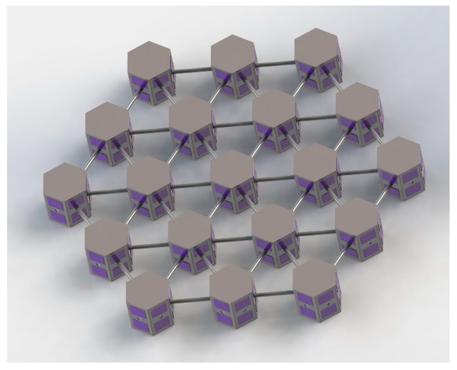
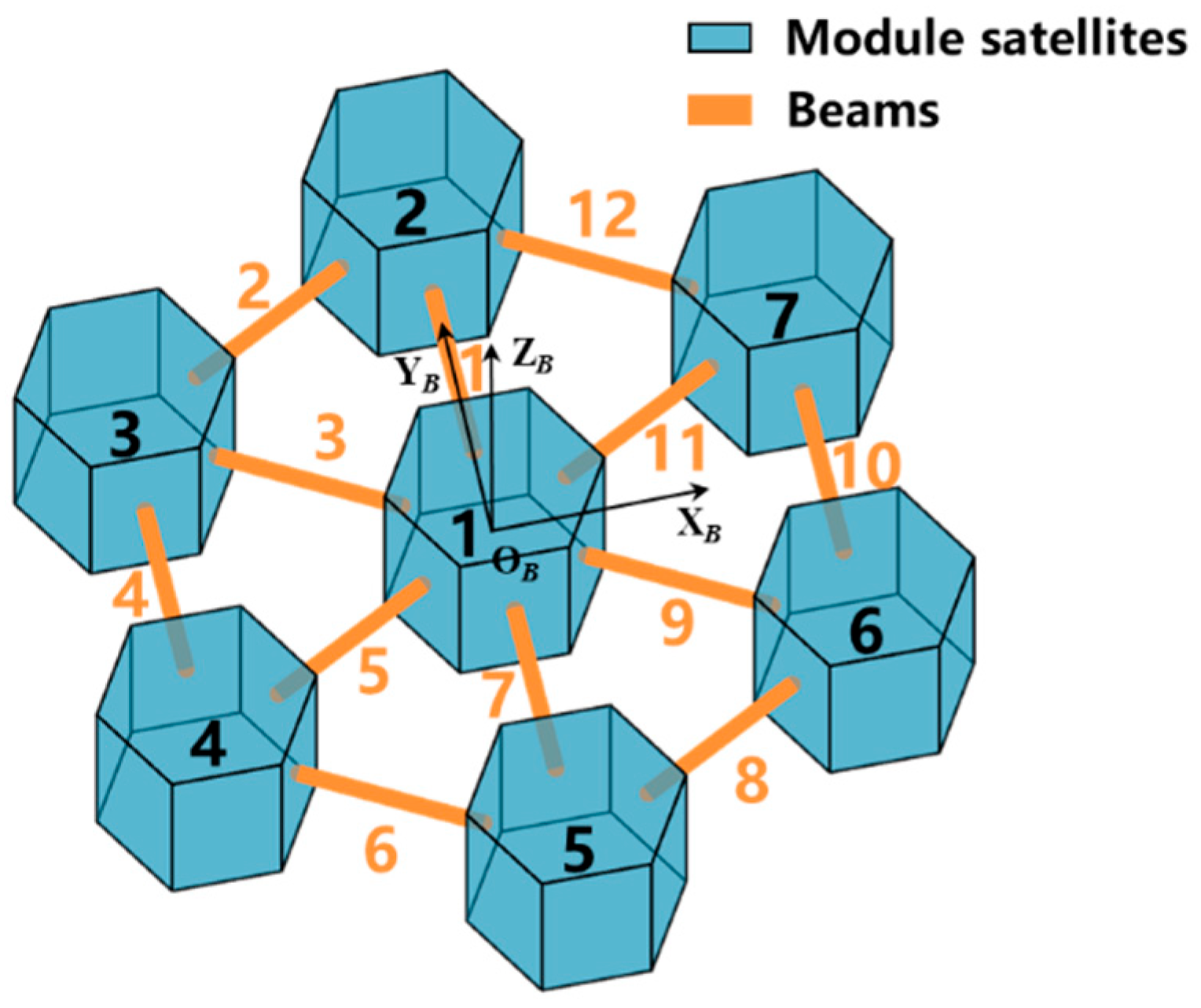
• Comparing Equations (54) and (56) demonstrates that the dynamic equations based on the direct assembly method of the ANCF have lower dimensions than those of the Lagrange multiplier method. Taking the constellation spacecraft with a mesh topology as shown in Figure 1 as an example, Figure 5 presents the relationship between the dynamic dimension and the number of modular satellites.

The following observations can be made from Figure 5:

1. The dynamic dimension of the system is approximately proportional to the number of modular satellites.

2. The dynamic dimension based on the direct assembly method of the ANCF is approximately half of that the Lagrange multiplier method.

Therefore, the proposed algorithm in this paper effectively reduces dimensionality disaster compared to the Lagrange multiplier method, leading to higher computational efficiency.

3. Force Analysis of Rigid–Flexible Composites in a Gravitational Field

The gravitational field is the fundamental mechanical environment for a composite spacecraft in orbit. The gravitational gradient effect is more pronounced on the composite structure due to the large-scale nature of the spacecraft. Additionally, the dynamic characteristics of the rigid and flexible components of the composite structure differ in the presence of a gravity field, leading to unique dynamic behaviors of the composite structure. The gravity acting on the rigid components of the composite structure can be simplified as a force passing through the center of mass and a gravity gradient torque. On the other hand, the gravity acting on the flexible components is a distributed force composed of the sum of gravity forces acting on each element. To simplify the model, without loss of generality, the following assumptions are made:

The orbital motion of the composite structure is decoupled from the vibrational motion of each spacecraft unit.

The scale of the flexible beam units is below the decimeter level, making the gravitational gradient effects on these units negligible compared to the effects on the larger composite structure and rigid bodies.

Each flexible beam unit undergoes small vibrations; thus, the gravity variations caused by the deformations of each unit can be disregarded.

The force analysis of the rigid–flexible coupled composite spacecraft in the gravitational field is depicted in the following figure:

In Figure 6, $O^{\mathrm{I}}-X^{\mathrm{I}}{Y}^{\mathrm{I}}{Z}^{\mathrm{I}}$ denotes the Earth-centered inertial coordinate system, $O^{\mathrm{C}}-X^{\mathrm{C}}{Y}^{\mathrm{C}}{Z}^{\mathrm{C}}$ represents the orbital translational coordinate system, and $O^{\mathrm{B}}-X^{\mathrm{B}}{Y}^{\mathrm{B}}{Z}^{\mathrm{B}}$ corresponds to the fixed-body coordinate system. The three axes of the orbital translational coordinate system align with those of the Earth-centered inertial coordinate system, while the origin moves along the reference trajectory in accordance with orbital dynamics. The dynamic modeling of the rigid–flexible coupled spacecraft is established in the orbital translational coordinate system, where the total external torque has the same form as that established in the inertial frame. However, the total external force must be separated into coupled accelerations.

The gravitational acceleration acting on any module can be determined using the universal law of gravitation:

$$a_{\mathrm{g}}^{\mathrm{I}}=-\mathrm{\mu }{\displaystyle \frac{r_{\mathrm{r}}^{\mathrm{I}}}{{‖r_{\mathrm{r}}^{\mathrm{I}}‖}^3}}$$

(57)

Here, μ represents the universal gravitational constant, and $r_{\mathrm{r}}^{\mathrm{I}}$ represents the position vector of the module’s center of mass in the inertial frame.

The translational acceleration of the orbital translational coordinate system, denoted as $O^{\mathrm{C}}-X^{\mathrm{C}}{Y}^{\mathrm{C}}{Z}^{\mathrm{C}}$, is given by the following:

$$a_{\mathrm{C}}^{\mathrm{I}}=-\mu {\displaystyle \frac{r_{\mathrm{C}}}{{‖r_{\mathrm{C}}‖}^3}}$$

(58)

Here, $r_{\mathrm{C}}$ represents the position of the origin of the orbital translational coordinate system in the Earth-centered inertial frame.

According to the principle of velocity superposition in mechanics, we can calculate the acceleration of the module in the translational coordinate system of the orbit as follows:

$$a_{\mathrm{g}}^{\mathrm{C}}=a_{\mathrm{g}}^{\mathrm{I}}-a_{\mathrm{C}}^{\mathrm{I}}$$

(59)

The corresponding gravity is given by the following:

$$F_{\mathrm{g}}^{\mathrm{C}}=m{a}_{\mathrm{g}}^{\mathrm{C}}$$

(60)

For any module, the torque exerted by the gradient of gravity is given by the following:

$$T_{\mathrm{g}}={\displaystyle \frac{3\mathrm{\mu }}{{‖r_{\mathrm{r}}^{\mathrm{I}}‖}^5}}\left(r_{\mathrm{r}}^{\mathrm{I}}\times I_{\mathrm{s}}{r}_{\mathrm{r}}^{\mathrm{I}}\right)$$

(61)

Here, $I_{\mathrm{s}}$ represents the moment of inertia matrix of the module.

The gravity experienced by any flexible beam element can be expressed as follows:

$$F_{\mathrm{g}}^{\mathrm{f}}={\displaystyle {\int }_V{S}^{\mathrm{T}}}\left(-\mathrm{\mu }{\displaystyle \frac{r_{\mathrm{f}}^{\mathrm{I}}}{{‖r_{\mathrm{f}}^{\mathrm{I}}‖}^3}}\right)dV$$

(62)

Here, $r_{\mathrm{f}}^{\mathrm{I}}$ represents the position of a point on the beam element in the Earth-centered inertial frame.

We can derive the gravity formulas for the overall assembly, rigid modules, and flexible beam elements by using Equations (60)–(62), respectively. Additionally, under assumption 3, when calculating Equation (62), we can approximate the flexible beam elements as rigid bodies to reduce computational complexity.

4. Verification of the Dynamic Response of Rigid–Flexible Composite Structures Through Simulation

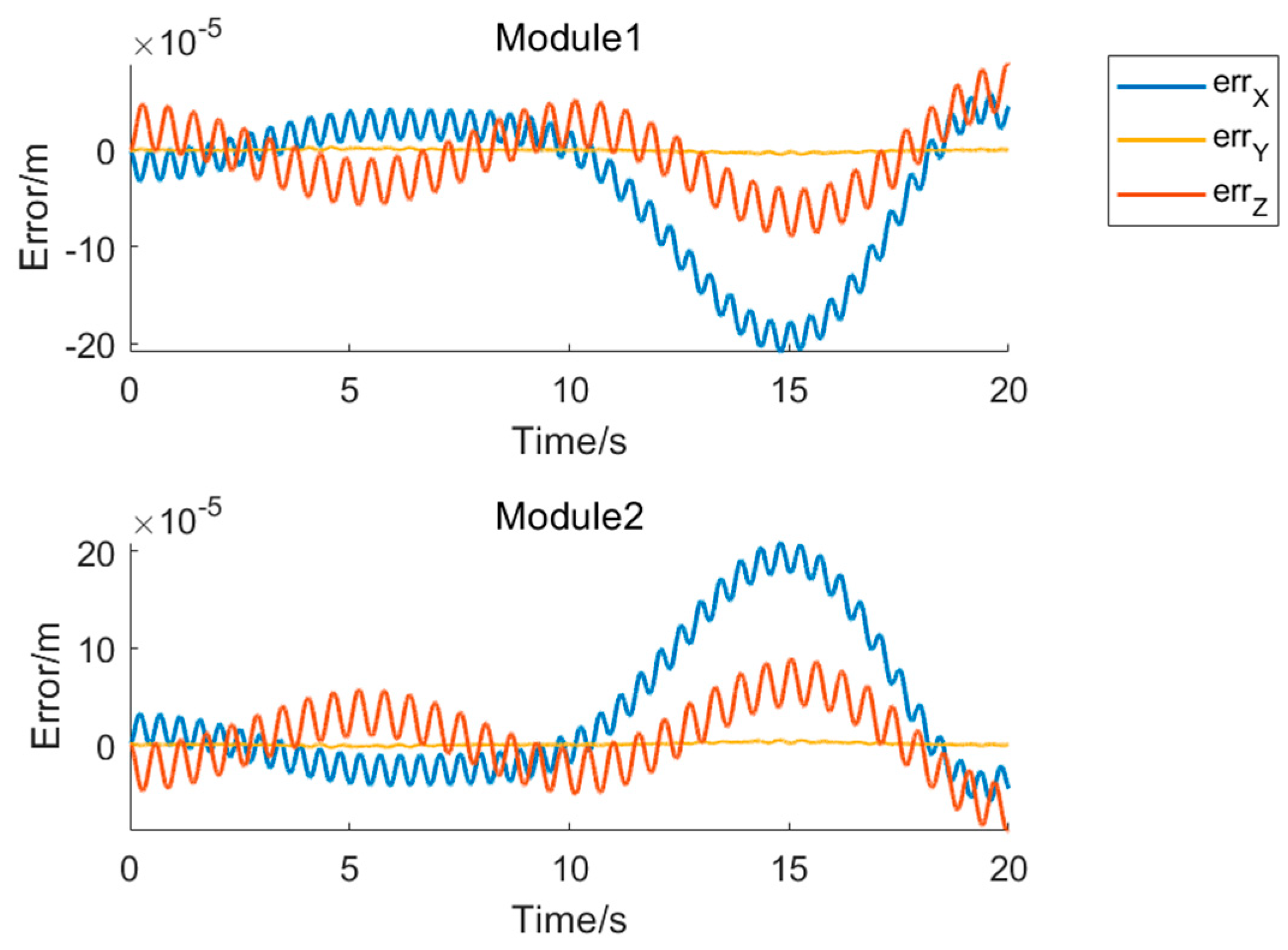
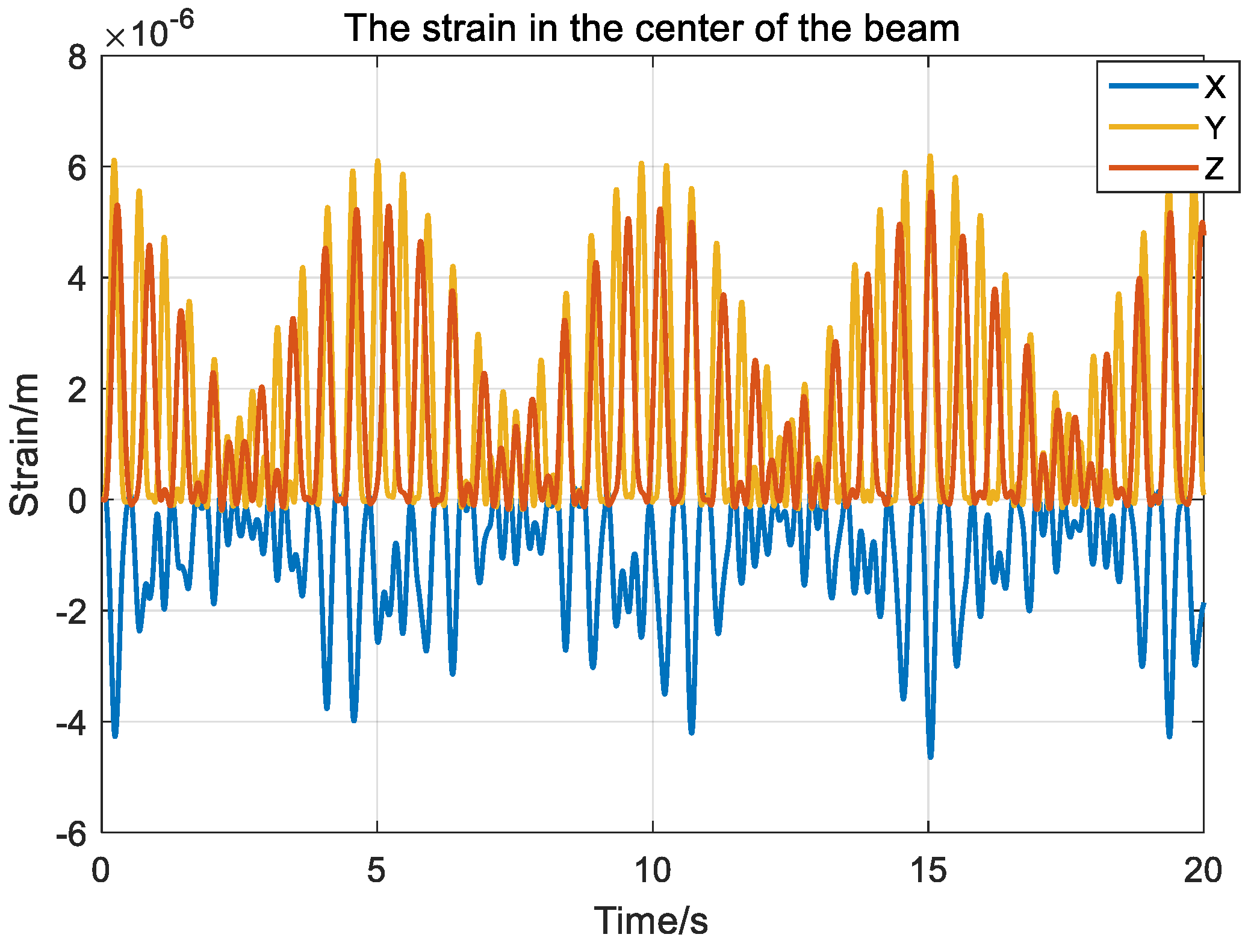
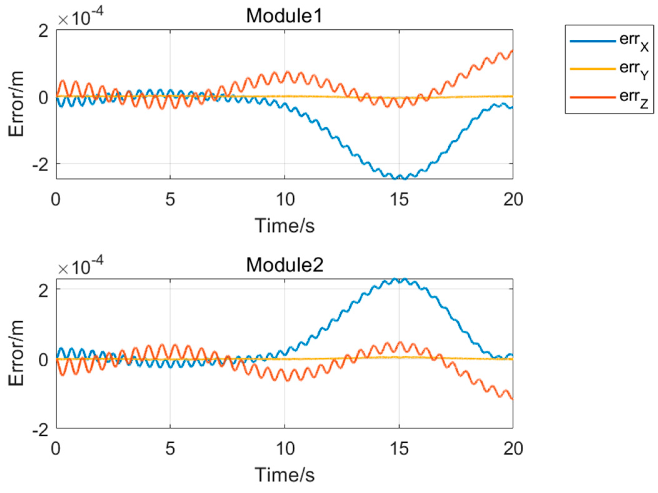
4.1. Analysis of Vibration Response in Dual-Module Composite Structures

To verify the accuracy and efficiency of the algorithm proposed in this paper, we conducted simulation verification using MATLAB on a dual-module dumbbell-shaped rigid–flexible composite spacecraft (shown in Figure 7). The computed results were compared and analyzed with the professional software ADAMS.

According to the previous assumption, the spacecraft module is enveloped by a regular hexagonal prism. The radius of the inscribed circle of its base hexagon is 0.5 m, and the height of the module is 0.8 m. The mass of the spacecraft is 50 kg, and its moment of inertia matrix is as follows:

$$I_s=\left[\begin{array}{ccc}2.1& 0& 0\\ 0& 3.2& 0\\ 0& 0& 1.8\end{array}\right]\left(\mathrm{kg}·{\mathrm{m}}^2\right)$$

(63)

The connecting flexible beam is a three-dimensional fully parameterized beam. It has a length $l=0.2 \mathrm{m}$, cross-sectional area $A=\left(0.01\times 0.01\right) {\mathrm{m}}^2$, Young’s modulus $E=2.1\times {10}^8\mathrm{Pa}$, Poisson’s ratio $v=0.27$, and density $\mathrm{\rho }=2700 {\mathrm{kg}/\mathrm{m}}^3$, and it is divided into two 0.1 m segments. The damping factor is set to 0, and the system does not include structural damping. In the MATLAB simulation, the rigid integrator ode23t is utilized with a relative tolerance of 10⁻³ and an absolute tolerance of 10⁻⁶.

A cyclic torque excitation, T_g, with a frequency of 0.1 Hz is applied along the X and Z axes in the fixed-body coordinate system of Module 1 and Module 2.

The errors of the two methods are shown below:

The curve below depicts the change in position of the combined center of mass.

The statistical analyses of the results of the algorithm used in this study and those of the ADAMS simulation are presented in the

Table 1. Error statistics of the algorithm used in this study and ADAMS simulation results.

Parameters	Module 1			Module 2
	X-Axis	Y-Axis	Z-Axis	X-Axis	Y-Axis	Z-Axis
Mean (m)	−3.63 × 10−5	−1.17 × 10−7	−6.63 × 10−6	3.63 × 10−5	1.17 × 10−7	6.63 × 10−6
Variance (m2)	5.72 × 10−9	1.94 × 10−12	1.32 × 10−9	5.72 × 10−9	1.94 × 10−12	1.32 × 10−9

.

Figure 8 presents the centroid position curves of the two modules, comparing the proposed method with ADAMS simulation results, while Figure 9 displays the corresponding error curves. The aforementioned curves and simulation results illustrate that the algorithm used in this study exhibits trends consistent with those of ADAMS and demonstrates a high level of conformity. The positional error remains within 0.2 mm throughout the 20 s simulation duration, with a variance of less than 6 × 10⁻⁹ m². Additionally, under symmetric excitation, the motion of Module 1 and Module 2 displays a center symmetric characteristic that aligns with the dynamic features of symmetric excitation. Figure 10 illustrates the center of mass of the assembly. In the ADAMS simulation, the center of mass remains at the origin with a data precision of seven significant digits, yielding an error of approximately 10⁻¹⁶ m. However, there may be occasional jumps at certain moments, with the maximum error not exceeding 10⁻⁸ m. In the MATLAB simulation results, the mean error of the center of mass is 1.35 × 10⁻¹⁴ m. Although this error is larger than that of ADAMS by two orders of magnitude, the absence of jumps indicates that the algorithm in this paper has better stability.

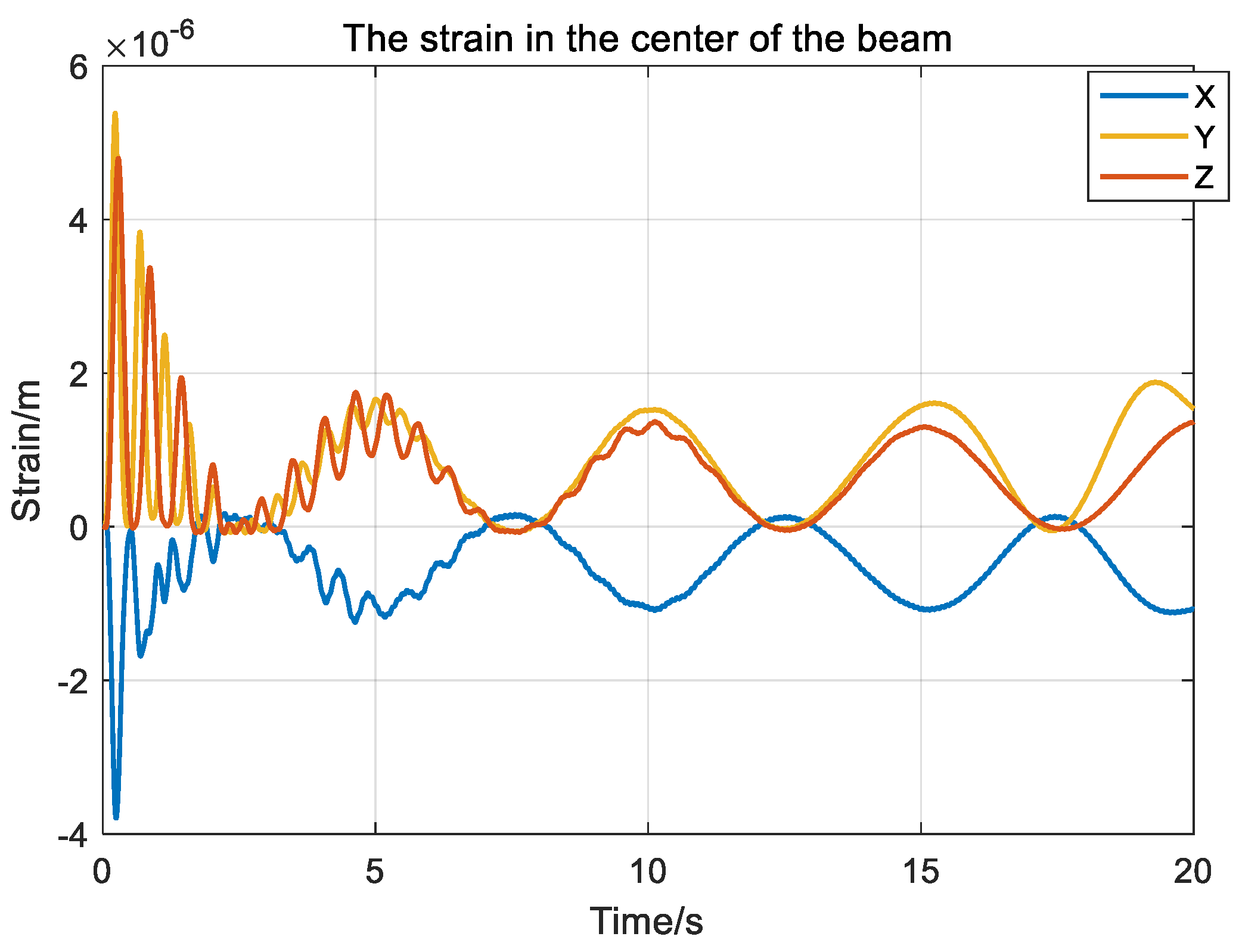
4.2. Analysis of the Impact of the Smoothing Factor on the Vibration of Dual-Module Assemblies

Section 2.1 demonstrates that the smoothing factor can suppress the high-frequency components of a system and increase the stability of the system. The objective of this case study is to verify the effect of the smoothing factor in the coupled rigid–flexible dynamic model. The simulation conditions are consistent with those discussed in Section 4.1. The corresponding dynamic simulation results for a smoothing factor of 0, 0.00001, and 0.0001 are presented below.

Figure 11 demonstrates that when the smoothing factor is zero, the strain magnitude at the midpoint of the beam oscillates within the range of 6 × 10⁻⁶ m and exhibits significant high-frequency components. Figure 12 demonstrates that when the smoothing factor is 0.00001, the strain amplitude at the midpoint of the beam progressively decreases, although noticeable high-frequency components still exist. Finally, Figure 13 indicates that when the smoothing factor is 0.00001, the strain amplitude at the midpoint of the beam decreases to within 2 × 10⁻⁶ m. Furthermore, the high-frequency components in the strain are suppressed, indicating greater system stability.

Comparing Figure 14 and Figure 15 reveals an increase in the error between the module displacement and ADAMS simulation results after a smoothing factor is introduced. Compared to the case with a smoothing factor of 0, the position error of the three axes increases when the smoothing factor is 0.00001, with a percentage ranging from 61.8% to 917.6%. However, these increases do not exceed an order of magnitude, and the overall error remains below 0.1 mm. The variance of the three axes also increases, ranging from 16.7% to 884.1%, with these increases also remaining within the same order of magnitude. When the smoothing factor is set to 0.0001, the error on the X-axis increases only by a range of 4.82% to 8.75%. The error on the Y-axis increases 837.4-fold but is still below 0.1 mm. Surprisingly, the error on the Z-axis decreases by 20.2%. The variance of the X-axis increases by a range of 1.5% to 3.1%, the variance of the Y-axis increases by approximately 400-fold, and the variance of the Z-axis changes by less than 1%.

The above indicates that the smoothing factor increases the error in the dynamic simulations. However, by selecting an appropriate smoothing factor, the stability of the dynamics can be enhanced while ensuring a certain level of accuracy.

Table 2. Comparison of position errors between smoothing factor of 0.00001 and ADAMS.

Parameters	Module 1			Module 2
	X-Axis	Y-Axis	Z-Axis	X-Axis	Y-Axis	Z-Axis
Mean (m)	−6.96 × 10−5	−9.82 × 10−7	2.32 × 10−5	5.88 × 10−5	7.20 × 10−7	−1.29 × 10−5
Variance (m2)	7.20 × 10−9	3.65 × 10−12	1.48 × 10−9	6.56 × 10−9	3.30 × 10−12	1.29 × 10−9

and

Table 3. Comparison of position errors between smoothing factor of 0.0001 and ADAMS.

Parameters	Module 1			Module 2
	X-Axis	Y-Axis	Z-Axis	X-Axis	Y-Axis	Z-Axis
Mean (m)	−3.78 × 10−5	−9.77 × 10−5	−5.28 × 10−6	3.95 × 10−5	9.81 × 10−5	5.28 × 10−6
Variance (m2)	5.80 × 10−9	7.55 × 10−9	1.32 × 10−9	5.89 × 10−9	7.80 × 10−9	1.32 × 10−9

present a statistical analysis of the module position errors in dynamic simulations compared to those of ADAMS under different smoothing factors. When the smoothing factor is constant, the position errors are all less than 0.1 mm, with a variance smaller than 10⁻⁸ m². As the smoothing factor increases from 10⁻⁵ to 10⁻⁴, the position errors slightly increase but remain below 0.1 mm, while the variance still remains below 10⁻⁸ m².

The simulation CPU time for different smoothing factors is shown in

Table 4. Simulation time statistics.

Smoothing Factor	0	0.00001	0.0001	0
Integrator	ODE45	ODE45	ODE45	ODE23t
CPU Time/s	16,156.9	15,242.3	4107.4	3517.8

. When the smoothing factor is 0.0001, the simulation time significantly decreases, approaching the efficiency of the ODE23t integrator designed for stiff differential equation systems. This validates that the smoothing factor can be controlled to adjust system stiffness and improve simulation efficiency.

In conclusion, incorporating a noise model in ANCF dynamics enables us to adjust the smoothing factor to balance accuracy, stability, and simulation efficiency. This expands the scope of applicability of this modeling method.

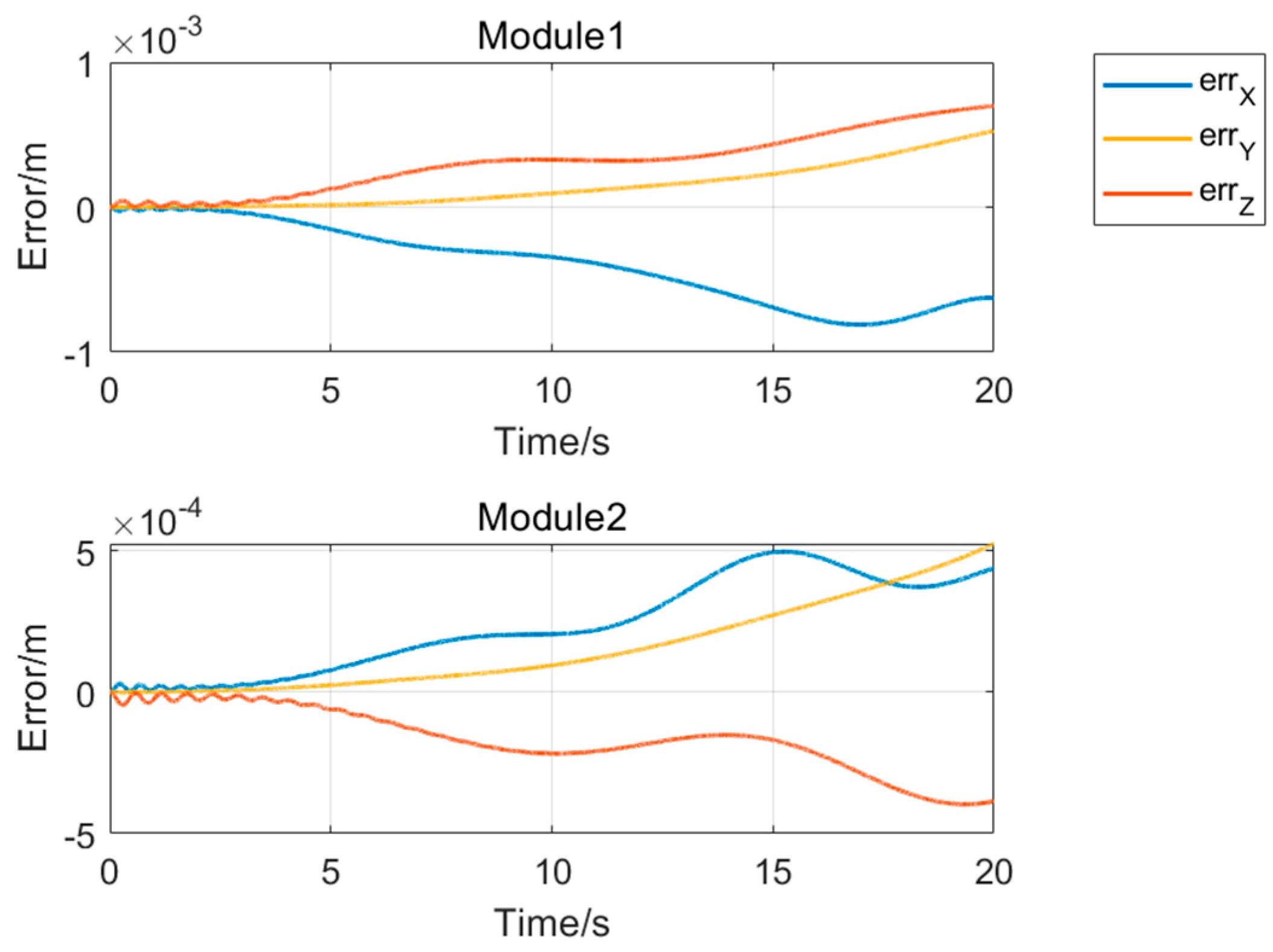
4.3. Vibration Response Analysis of a Seven-Module Assembly in a Gravitational Environment

In this analysis, the dynamic characteristics of rigid–flexible coupled spacecraft under the constraints of orbital dynamics are examined and analyzed, with particular consideration given to the influence of gravity gradient torque in a gravity environment. Additionally, the vibration characteristics of the combined spacecraft in orbit are examined through Fourier transformation analysis. The initial reference orbit is a circular orbit at an altitude of 500 km, with the six orbital elements shown in

Table 5. The initial reference orbit’s six orbital elements.

Semi-Major Axis/km	Eccentricity	Inclination/°	RAAN/°	Argument of Perigee/°
6878.137	0.001	0	0	0

.

The combined spacecraft comprises seven rigid body modules, as depicted in Figure 16. The length of the connecting beams is 1 m, while the parameters for the remaining rigid and flexible beam units are the same as those in Section 4.1.

The axial displacement vibrations of the connecting beam’s end nodes are depicted in Figure 17.

The vibration frequencies of the end nodes were obtained through Fourier transformation and are shown in Figure 18.

The above figure reveals that the connecting beams experience vibrations at the nanometer level in a gravity environment. Through frequency domain analysis, the first-order frequency is determined to be 4.4 Hz, the second-order frequency is 5.6 Hz, and the third-order frequency is 6.35 Hz. The presence of gravity in the environment induces vibrations in the coupled rigid–flexible combined spacecraft. Although the amplitude is minimal, the low frequencies pose a risk of resonance when subjected to disturbances from other space factors.

Based on the aforementioned simulation, the length of the connecting beams is increased to 10 m. The axial displacement vibration of the end nodes of each connecting beam is shown in Figure 19, and the amplitude–frequency characteristics are depicted in Figure 20. The first three resonant frequencies of the end node vibrations are 1.35 Hz, 1.75 Hz, and 2.05 Hz. Evidently, increasing the length of the beam results in a decrease in the characteristic frequencies. Therefore, larger-scale coupled rigid–flexible spacecraft exhibit lower characteristic frequencies and poorer stability.

5. Conclusions

In this paper, dynamic modeling of a mesh topology rigid–flexible coupled spacecraft is addressed. A direct assembly method based on the absolute nodal coordinate formulation (ANCF) is proposed that reduces the dimension of dynamics by half when compared to the Lagrange multiplier method. Additionally, for the first time, a noise reduction model for flexible beam elements is applied to the rigid–flexible coupling dynamic model. Furthermore, the external forces experienced in the gravitational environment are transformed and incorporated into the rigid–flexible coupling dynamics, establishing the fundamental dynamic model of the spacecraft in orbit. The accuracy of the proposed algorithm is validated by comparing the proposed algorithm with ADAMS dynamics, and mm-level precision is achieved. By adjusting the smoothing factor, the simulation efficiency can be improved several times while maintaining precision in the mm-level range. Under the influence of gravity, the combined spacecraft with a mesh topology configuration exhibits slight vibrations, with identical characteristic frequencies of each connecting flexible beam. Moreover, the characteristic frequency decreases as the length of the connecting beam increases. In conclusion, the proposed direct assembly dynamic modeling method based on ANCF for rigid–flexible coupling can be used for dynamic modeling in the space environment and can analyze the characteristic frequencies of different configurations, providing references for the configuration design of combined spacecraft.

References

1. He, G.; Cao, D.; Wei, J.; Cao, Y.; Chen, Z. Study on analytical global modes for a multi-panel structure connected with flexible hinges. Appl. Math. Model. 2021, 91, 1081–1099. [Google Scholar] [CrossRef]
2. Wang, E.; Wu, S.; Liu, Y.; Wu, Z.; Liu, X. Distributed vibration control of a large solar power satellite. Astrodynamics 2019, 3, 189–203. [Google Scholar] [CrossRef]
3. Shabana, A.A. An Absolute Nodal Coordinate Formulation for the Large Rotation and Deformation Analysis of Flexible Bodies; Technical Report; Department of Mechanical Engineering, University of Illinois at Chicago: Chicago, IL, USA, 1996. [Google Scholar]
4. Zwölfer, A.; Gerstmayr, J. The nodal-based floating frame of reference formulation with modal reduction. Acta Mech. 2020, 232, 835–851. [Google Scholar] [CrossRef]
5. Sun, J.; Tian, Q.; Hu, H.; Pedersen, N.L. Axially variable-length solid element of absolute nodal coordinate formulation. Acta Mech. Sin. 2019, 35, 653–663. [Google Scholar] [CrossRef]
6. Shabana, A.A.; Schwertassek, R. Equivalence of the floating frame of reference approach and finite element formulations. Int. J. Non-Linear Mech. 1998, 33, 417–432. [Google Scholar] [CrossRef]
7. Shabana, A.A. Computational Continuum Mechanics, 2nd ed.; Cambridge University Press: New York, NY, USA, 2012. [Google Scholar] [CrossRef]
8. Luo, C.Q.; Sun, J.L.; Wen, H.; Jin, D.P. Dynamics of a tethered satellite formation for space exploration modeled via ANCF. Acta Astronaut. 2020, 177, 882–890. [Google Scholar] [CrossRef]
9. Htun, T.Z.; Suzuki, H.; Garcia-Vallejo, D. Dynamic modeling of a radially multilayered tether cable for a remotely-operated underwater vehicle (ROV) based on the absolute nodal coordinate formulation (ANCF). Mech. Mach. Theory 2020, 153, 103961. [Google Scholar] [CrossRef]
10. Otsuka, K.; Makihara, K. Absolute Nodal Coordinate Beam Element for Modeling Flexible and Deployable Aerospace Structures. AIAA J. 2019, 57, 1344–1346. [Google Scholar] [CrossRef]
11. Westin, C.; Irani, R.A. Efficient semi-implicit numerical integration of ANCF and ALE-ANCF cable models with holonomic constraints. Comput. Mech. 2023, 71, 789–800. [Google Scholar] [CrossRef]
12. Desai, C.S.; Kundu, T.; Lei, X. Introductory Finite Element Method. Appl. Mech. Rev. 2002, 55, 284–288. [Google Scholar] [CrossRef]
13. Yu, L.; Zhao, Z.; Tang, J.; Ren, G. Integration of absolute nodal elements into multibody system. Nonlinear Dyn. 2010, 62, 931–943. [Google Scholar] [CrossRef]
14. Hu, J.; Wang, T. A recursive absolute nodal coordinate formulation with O(n) algorithm complexity. Chin. J. Theor. Appl. Mech. 2016, 48, 1172–1183. [Google Scholar] [CrossRef]
15. Kim, E.; Cho, M. Design of a planar multibody dynamic system with ANCF beam elements based on an element-wise stiffness evaluation procedure. Struct. Multidiscip. Optim. 2018, 58, 1095–1107. [Google Scholar] [CrossRef]
16. Ren, H.; Zhou, P. Implementation details of DAE integrators for multibody system dynamics. J. Dyn. Control 2021, 19, 1–28. [Google Scholar]
17. Yan, Y.; Chen, W.; Wang, C.; Wise, S.M. A second-order energy stable BDF numerical scheme for the Cahn-Hilliard equation. Commun. Comput. Phys. 2018, 23, 572–602. [Google Scholar] [CrossRef]
18. Zhang, H.; Zhang, R.; Zanoni, A.; Masarati , P. Performance of implicit A-stable time integration methods for multibody system dynamics. Multibody Syst. Dyn. 2022, 54, 263–301. [Google Scholar] [CrossRef]
19. Jia, C.; Su, H.; Guo, W.; Masarati, P. An Unconditionally Stable Integration Method for Structural Nonlinear Dynamic Problems. Mathematics 2023, 11, 2987. [Google Scholar] [CrossRef]
20. Amiri-Hezaveh, A.; Ostoja-Starzewski, M. A convolutional-iterative solver for nonlinear dynamical systems. Appl. Math. Lett. 2022, 130, 107990. [Google Scholar] [CrossRef]
21. Hanafi, M.R.; Babaei, M.; Narjabadifam, P. New Formulation for dynamic analysis of nonlinear time-history of vibrations of structures under earthquake loading. J. Civ. Environ. Eng. 2023, 54, 22–35. [Google Scholar] [CrossRef]
22. Yang, Y.; Chen, Y.; Zhang, B.; Xie, F.; Qiu, D. A Time-varying Amplitude and Frequency Description Method of Instantaneous Signal in Power System Based on HHT. In Proceedings of the 2023 IEEE 6th International Electrical and Energy Conference (CIEEC), Hefei, China, 12–14 May 2023; IEEE: New York, NY, USA, 2023; pp. 1255–1260. [Google Scholar] [CrossRef]
23. Qi, Z.; Cao, Y.; Wang, G. Model smoothing methods in numerical analysis of flexible multibody systems. Chin. J. Theor. Appl. Mech. 2018, 50, 863–870. [Google Scholar] [CrossRef]
24. Zhang, Z.; Zhou, X.; Mao, H.; Song, H. Model denoising based on absolute node coordinate method. J. Vib. Shock 2021, 40, 139–146. [Google Scholar]
Figure 1. Schematic diagram of rigid–flexible coupled spacecraft.
Aerospace 12 00207 g001
Figure 2. Fully parameterized beam element.
Aerospace 12 00207 g002
Figure 3. Relationship between three configurations in ANCF.
Aerospace 12 00207 g003
Figure 4. A conceptual diagram of the combined spacecraft with a rigid–flexible body assembly.
Aerospace 12 00207 g004
Figure 5. The relationship between the system’s dynamic dimension and the number of modular satellites.
Aerospace 12 00207 g005
Figure 6. The gravitational forces acting on the composite spacecraft.
Aerospace 12 00207 g006
Figure 7. The dumbbell-shaped configuration of the composite spacecraft.
Aerospace 12 00207 g007
Figure 8. A comparison of the displacement simulation results of the dual module under cyclic excitation in MATLAB R2024b and ADAMS 2024.1.
Aerospace 12 00207 g008
Figure 9. The difference in displacement simulation results between MATLAB and ADAMS for the dual module under cyclic excitation.
Aerospace 12 00207 g009
Figure 10. Graph of combined center of mass variation.
Aerospace 12 00207 g010
Figure 11. The strain variation curve at the midpoint of the beam for a smoothing factor of 0.
Aerospace 12 00207 g011
Figure 12. The strain variation curve at the midpoint of the beam for a smoothing factor of 0.00001.
Aerospace 12 00207 g012
Figure 13. The strain variation curve at the midpoint of the beam for a smoothing factor of 0.0001.
Aerospace 12 00207 g013
Figure 14. Error curve of module position for smoothing factor of 0.00001.
Aerospace 12 00207 g014
Figure 15. Error curve of module position for smoothing factor of 0.0001.
Aerospace 12 00207 g015
Figure 16. The configuration of the combined spacecraft with seven modules.
Aerospace 12 00207 g016
Figure 17. The axial displacement of the end nodes of the flexible beam (1 m).
Aerospace 12 00207 g017
Figure 18. The amplitude–frequency characteristics of the axial vibrations at the end nodes of the flexible beam (1 m).
Aerospace 12 00207 g018
Figure 19. The axial displacement of the end nodes of the flexible beam (10 m).
Aerospace 12 00207 g019
Figure 20. The amplitude–frequency characteristics of the axial vibrations at the end nodes of the flexible beam (10 m).
Aerospace 12 00207 g020