An Initial Trajectory Design for the Multi-Target Exploration of the Electric Sail

Abstract

The electric sail (E-sail), as an emerging propulsion system with an infinite specific impulse, is particularly suitable for ultra-long-distance multi-target deep-space exploration missions. If multiple gravity assists are considered during the exploration process, it can effectively improve the exploration efficiency of the E-sail. This paper proposes a fast optimization algorithm for deep-space multi-target exploration trajectories for the E-sail, which achieves the exploration of multiple celestial bodies and solar-system boundaries in one flight, and introduces a gravity assist to improve the flight speed of the E-sail during the exploration process. By comparing simulation examples under different conditions, the effectiveness of the algorithm proposed in this paper has been demonstrated. This is of great significance for the initial rapid design of complex deep-space exploration missions such as the E-sail multi-target exploration.

1. Introduction

Exploring important celestial bodies and boundaries of the solar system is of great significance [1], as it can help humanity gain a deeper understanding of the solar system [2]. However, ultra-long-distance deep-space exploration missions not only make the initial mission design very complex, but also require efficient propulsion systems. Traditional pulse engines have a low specific impulse, require a large amount of fuel consumption, and are costly. The E-sail generates thrust by utilizing the dynamic pressure of the solar wind, without the need for fuel consumption, and has an infinite specific impulse [3,4,5,6]. Current research assumes to continuously steer the E-sail and neglects uncertainties associated with solar wind properties [7,8]. It can provide continuous thrust throughout the entire mission cycle, making it very suitable for ultra-long-distance and long-term deep-space exploration missions [9,10,11].

Due to the continuous and low thrust generated by the E-sail, it takes a long time for the E-sail to reach a high flight speed. Therefore, considering the gravitational assistance of celestial bodies during flyby exploration can quickly increase the flight speed of the E-sail [12]. However, this makes the efficient design and optimization of its flight trajectory extremely challenging, and the strong nonlinearity of the problem makes the solving process very difficult. The traditional direct and indirect methods [13,14] used for trajectory optimization have low computational efficiency and require high-precision optimization initial values [15,16,17]. Therefore, in recent years, the shape-based methods [18,19] have been proposed to design the transfer trajectory of such continuous low-thrust spacecraft [20,21]. The shape-based methods have high computational efficiency [22,23,24] and can be quickly optimized to obtain high-precision transfer trajectories [25,26,27,28]. Petropoulos et al. [29] first proposed using exponential sine functions to describe the flight trajectory of the spacecraft, and then optimizing coefficients to satisfy the corresponding constraints. Taheri and Abdelkhalik proposed using the Finite Fourier Series shape-based method to obtain two-dimensional [30,31] and three-dimensional [32] transfer trajectories of the low-thrust spacecraft detecting planets or asteroids. Fan et al. [20] also demonstrated that for asteroid exploration, the Bezier shape-based method can achieve better performance indicators in a shorter time compared to the Finite Fourier Series shape-based method; compared with the direct method, the Bezier shape-based method can obtain feasible solutions with very little difference in performance indicators in a very short time. Unlike trajectory design in asteroid exploration, in the trajectory optimization problem of the joint exploration of multiple celestial bodies and solar-system boundaries, the constraints are more complex. The final arrival point of the E-sail is not a specific celestial body, but the solar-system boundary. At this point, the E-sail has either flown to the solar-system boundary [33] or obtained the energy to fly to the solar-system boundary [10]. At the same time, the influence of gravity-assist processes on trajectory design also needs to be considered. Therefore, the trajectory optimization process of the multi-target exploration problem studied in this paper is more complex.

Therefore, this paper uses the Bezier shape-based method to design the transfer trajectory of the E-sail multi-target and solar-system boundary exploration with the gravity assist, and proves the effectiveness of the proposed algorithm by comparing multiple complex exploration examples. The organizational structure of the subsequent chapters is as follows: in Section 2, the corresponding mathematical models are established; Section 3 provides a brief description of the Bezier shape-based method; in Section 4, various simulation examples are compared; and Section 5 provides the conclusion.

2. Problem Description

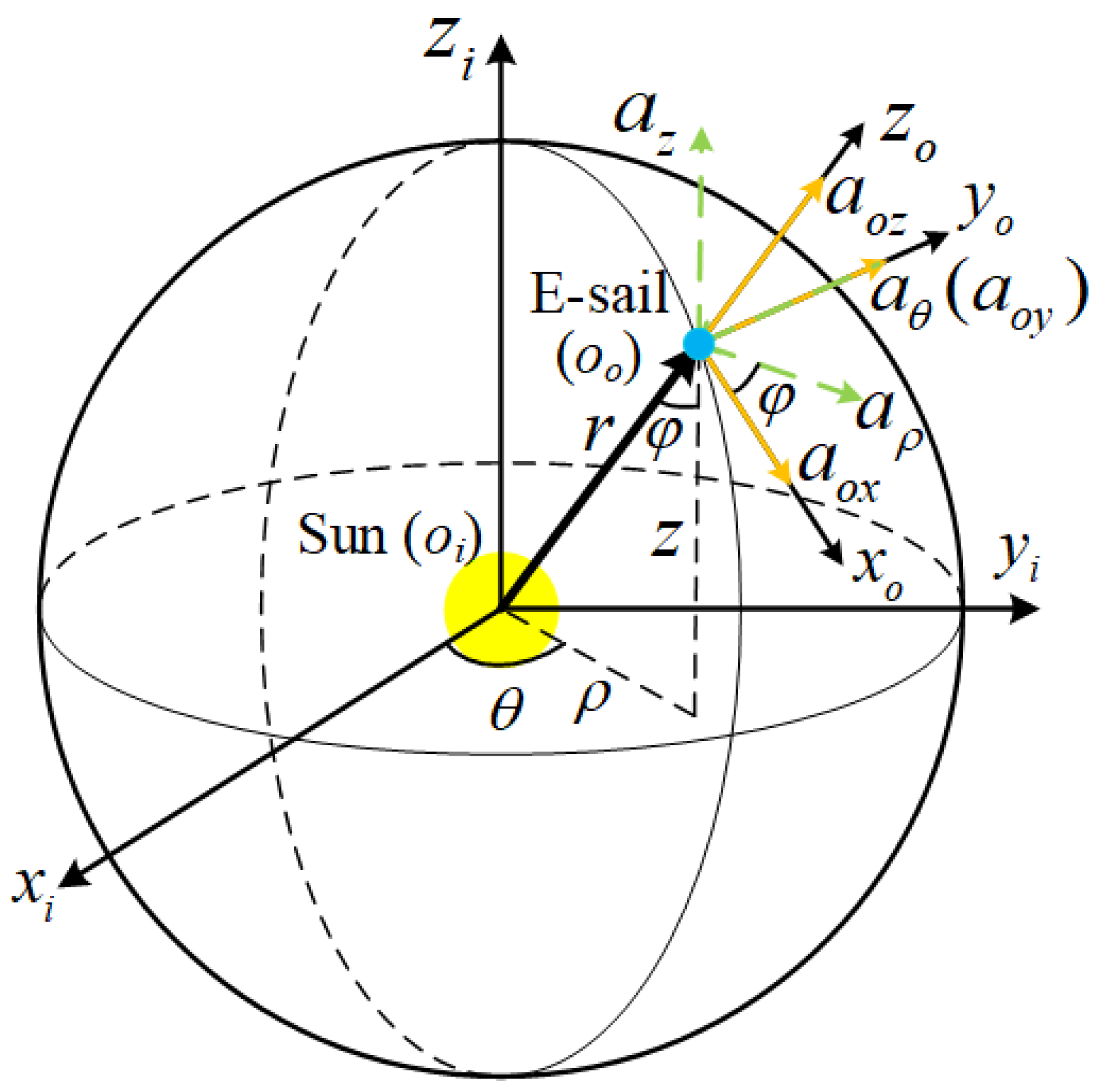
2.1. Coordinate Systems

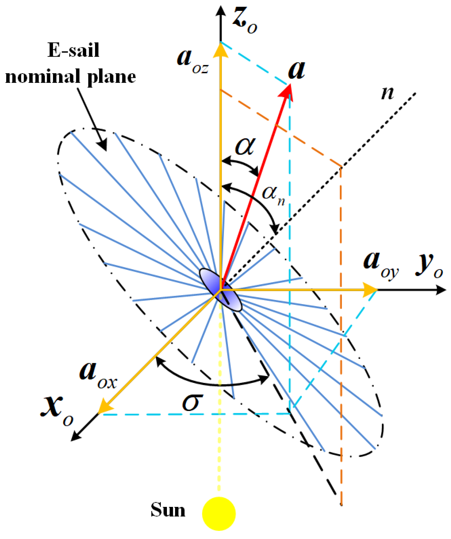
As shown in Figure 1 and Figure 2, this section uses $o_i{x}_i{y}_i{z}_i$, $o_o{x}_o{y}_o{z}_o$ and $(\rho ,\theta ,z)$ to describe the E-sail, where $o_i{x}_i{y}_i{z}_i$ is the heliocentric ecliptic inertial system, $o_o{x}_o{y}_o{z}_o$ is the orbital reference system, and $(\rho ,\theta ,z)$ is a set of cylindrical coordinates. The origin $o_i$ is the center of the sun, with the positive $x_i$-axis pointing towards the vernal equinox at epoch J2000.0, the positive $z_i$-axis perpendicular to the ecliptic plane at J2000.0 and pointing towards the north pole of the ecliptic, and the $y_i$-axis forming a right-handed system with the $x_i$-axis and $z_i$-axis. The $o_o$ is located in the center of mass of the E-sail, the $z_o$-axis points from the sun towards the E-sail, the $y_o$-axis is perpendicular to the $z_o$-axis and the normal axis of the ecliptic plane, the $y_o$-axis is perpendicular to the ($z_o$, $z_i$) plane and has the same direction as the E-sail inertial velocity, and the $x_o$-axis completes the right-handed system. $\rho$ is the distance between the projection point of the E-sail on the $x_i{o}_i{y}_i$ plane and the origin, $\theta$ is the azimuth angle, z is the height of the E-sail. $a_{ox}$, $a_{oy}$, $a_{oz}$, $a_{\rho }$, $a_{\theta }$, and $a_z$ are the corresponding propulsive acceleration components. n is the unit vector perpendicular to the nominal plane of the sail, ${\alpha }_n\in \left[0,\pi /2\right]$ is the pitch angle, $\sigma \in \left[0,2\pi \right]$ is the angle between the $x_o$-axis and the component of $\mathit{n}$ in the $o_o{x}_o{y}_o$ plane, and $\alpha$ is the angle between the propulsive acceleration vector $\mathit{a}$ and the $z_o$-axis.

2.2. Thrust Model

The analytical propulsive acceleration components of the E-sail in $o_o{x}_o{y}_o{z}_o$ are

$$\left[\begin{array}{c}{a}_{ox}\\ a_{oy}\\ a_{oz}\end{array}\right]={\displaystyle \frac{a_c{r}_{\oplus }\kappa }{2r}}\left[\begin{array}{c}\cos {\alpha }_n\sin {\alpha }_n\cos \sigma \\ \cos {\alpha }_n\sin {\alpha }_n\sin \sigma \\ {\cos }^2{\alpha }_n+1\end{array}\right]$$

(1)

where $r=\sqrt{{\rho }^2+z^2}$, $r_{\oplus }=1\mathrm{au}$, $a_c$ is the characteristic acceleration, and $\kappa \in \left[0,1\right]$ is the thrust coefficient of the E-sail that is assumed to be continuously adjustable, thereby continuously changing thrust magnitude. From Figure 1, it can be seen that the propulsion acceleration components of the E-sail in $(\rho ,\theta ,z)$ and $o_o{x}_o{y}_o{z}_o$ only need to rotate $\phi$ around the $y_o$-axis, thus obtaining:

$$\left[\begin{array}{c}{a}_{\rho }\\ a_{\theta }\\ a_z\end{array}\right]=\left[\begin{array}{ccc}\cos \phi & 0& \sin \phi \\ 0& 1& 0\\ -\sin \phi & 0& \cos \phi \end{array}\right]\left[\begin{array}{c}{a}_{ox}\\ a_{oy}\\ a_{oz}\end{array}\right]=\left[\begin{array}{c}\cos \phi a_{ox}+\sin \phi a_{oz}\\ a_{oy}\\ -\sin \phi a_{ox}+\cos \phi a_{oz}\end{array}\right]$$

(2)

where $\sin \phi =\rho /\sqrt{{\rho }^2+z^2}$ and $\cos \phi =z/\sqrt{{\rho }^2+z^2}$.

The equations of motion of the E-sail are

$$\begin{array}{cc}\hfill & \ddot{\rho }-\rho {\dot{\theta }}^2+{\mu }_{\odot }\rho /r^3=a_{\rho }\hfill \\ \hfill & \rho \ddot{\theta }+2\dot{\rho }\dot{\theta }=a_{\theta }\hfill \\ \hfill & \ddot{z}+{\mu }_{\odot }z/r^3=a_z\hfill \end{array}$$

(3)

where ${\mu }_{\odot }$ is the gravitational parameter of the sun.

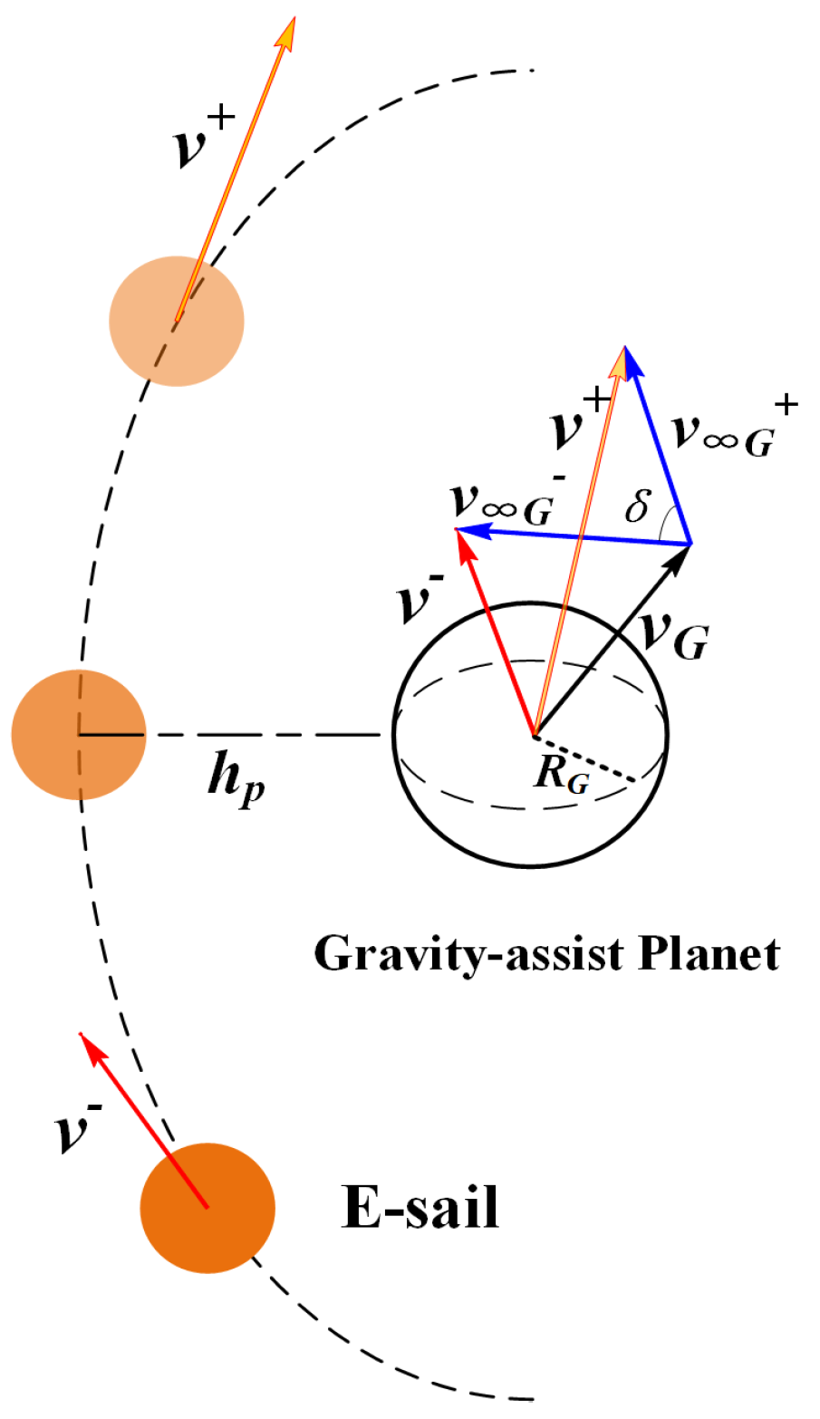
2.3. Gravity-Assist Models

In $o_i{x}_i{y}_i{z}_i$, when the position of the gravity-assist planet coincides with the position of the E-sail, the gravity-assist process is instantaneously completed, ignoring all disturbances. The gravity-assisted process is shown in Figure 3, and the kinematic equation is as follows:

$$\begin{array}{cc}\hfill & {\mathit{v}}_{\infty G}^{-}={\mathit{v}}^{-}-{\mathit{v}}_G\hfill \\ \hfill & {\mathit{v}}_{\infty G}^{+}={\mathit{v}}^{+}-{\mathit{v}}_G\hfill \\ \hfill & \parallel {\mathit{v}}_{\infty G}^{-}\parallel =\parallel {\mathit{v}}_{\infty G}^{+}\parallel =v_{\infty }\hfill \\ \hfill & \delta =arccos\left({\displaystyle \frac{{\mathit{v}}_{\infty G}^{+}·{\mathit{v}}_{\infty G}^{-}}{v_{\infty }^2}}\right)\hfill \\ \hfill & h_p={\displaystyle \frac{{\mu }_G}{v_{\infty }^2}}\left({\displaystyle \frac{1}{sin\left(\frac{\delta }{2}\right)}}-1\right)-R_G\hfill \end{array}$$

(4)

where ${\mu }_G$, $R_G$, and ${\mathit{v}}_G$ are the gravitational parameter, the average radius, and the heliocentric velocity vector of the gravity-assist planet, respectively. Before and after the gravity-assist process, ${\mathit{v}}^{-}$ and ${\mathit{v}}^{+}$ are the heliocentric velocity vectors of the E-sail, and ${\mathit{v}}_{\infty G}^{-}$ and ${\mathit{v}}_{\infty G}^{+}$ are the relative velocity vectors of the gravity-assist planet and the E-sail. $v_{\infty }$ is the modulus of ${\mathit{v}}_{\infty G}^{-}$ and ${\mathit{v}}_{\infty G}^{+}$, $\delta$ is the angle between ${\mathit{v}}_{\infty G}^{-}$ and ${\mathit{v}}_{\infty G}^{+}$, and $h_p$ is the gravity-assist pericenter altitude.

2.4. Constraint Conditions

By (1), we can obtain

$$\begin{array}{cc}\hfill a_{ox}^2+a_{oy}^2& ={\left({\displaystyle \frac{a_c{r}_{\oplus }\kappa }{2r}}\right)}^2{\cos }^2\left({\alpha }_n\right){\sin }^2\left({\alpha }_n\right)\hfill \\ \hfill {\cos }^2\left({\alpha }_n\right)& =\left(2r{a}_{oz}\right)/\left(a_c{r}_{\oplus }\kappa \right)-1\hfill \end{array}$$

(5)

Through (5), the equation about $\kappa$ can be obtained as follows:

$$2{\left({\displaystyle \frac{a_c{r}_{\oplus }}{2r}}\right)}^2{\kappa }^2-3\left({\displaystyle \frac{a_c{r}_{\oplus }{a}_{oz}}{2r}}\right)\kappa +(a_{ox}^2+a_{oy}^2+a_{oz}^2)=0$$

(6)

When ${\alpha }_n=0(a_{ox}=a_{oy}=0)$, solving (6) yields:

$$\kappa ={\displaystyle \frac{r\left(3a_{oz}-\sqrt{a_{oz}^2-8a_{ox}^2-8a_{oy}^2}\right)}{2a_c{r}_{\oplus }}}$$

(7)

Through (2), $\kappa$ can be expressed in the following form:

$$\kappa ={\displaystyle \frac{r·\left(3\left(\sin \phi ·a_{\rho }+\cos \phi ·a_z\right)-\sqrt{D}\right)}{2a_c{r}_{\oplus }}}$$

(8)

where

$$\begin{array}{cc}\hfill D=& {(\sin \phi ·a_{\rho }+\cos \phi ·a_z)}^2-8a_{\theta }^2-8{(\cos \phi ·a_{\rho }-\sin \phi ·a_z)}^2\ge 0\hfill \end{array}$$

When the E-sail performs orbit transfer, the following boundary conditions need to be met:

$$\begin{array}{cccc}\rho (\tau =0)={\rho }_i& \rho (\tau =1)={\rho }_f& {\rho }^{\prime }(\tau =0)=T{\dot{\rho }}_i& {\rho }^{\prime }(\tau =1)=T{\dot{\rho }}_f\\ \theta (\tau =0)={\theta }_i& \theta (\tau =1)={\theta }_f& {\theta }^{\prime }(\tau =0)=T{\dot{\theta }}_i& {\theta }^{\prime }(\tau =1)=T{\dot{\theta }}_f\\ z(\tau =0)=z_i& z(\tau =1)=z_f& z^{\prime }(\tau =0)=T{\dot{z}}_i& z^{\prime }(\tau =1)=T{\dot{z}}_f\end{array}$$

(9)

where $0\le \tau =t/T\le 1$, T is the total flight time, superscrs the total flight time, superscript ^˙ and ^′ denote the derivative with respect to the flight time t and $\tau$, respectively, and subscripts “i” and “f” denote the initial and final conditions, respectively.

In the problem of escaping the solar system studied in this paper, it is required that E-sail ultimately obtains the energy to fly to the boundary of the solar system [10]:

$${\epsilon }_f\triangleq {\displaystyle \frac{v_f^2}{2}}-{\displaystyle \frac{\mu }{r_f}}={\displaystyle \frac{V_{\infty }^2}{2}}$$

(10)

where $v_f$ is the flight speed of the E-sail when it reaches the condition of escaping the solar system, and $V_{\infty }$ is the hyperbolic transition speed of the E-sail. When $V_{\infty }=0$, it can be considered that the E-sail has reached the condition necessary to escape from the solar system.

3. The Bezier Shape-Based Method

In the Bezier shape-based method, the coordinates of the E-sail are expressed in the following form:

$$\begin{array}{cc}\hfill \zeta \left(\tau \right)& =\sum _{j=0}^{n_{\zeta }}{B}_{\zeta ,j}\left(\tau \right)P_{\zeta ,j},\zeta =\rho ,\theta ,z\hfill \end{array}$$

(11)

where $n_{\zeta }$ are the orders of the Bezier curve, and $P_{\zeta ,j}(j\in \left[0,n_{\zeta }\right])$ are the unknown Bezier coefficients. The unknown Bezier coefficients are variables that need to be optimized, while the Bezier orders can be manually adjusted. $B_{\zeta ,j}\left(\tau \right)$ are as follows:

$$\begin{array}{ccc}\hfill B_{\zeta ,j}\left(\tau \right)& ={\displaystyle \frac{n_{\zeta }!}{j!(n_{\zeta }-j)!}}{\tau }^j{(1-\tau )}^{n_{\zeta }-j}\hfill & \hfill j\in \left[0,n_{\zeta }\right]\end{array}$$

(12)

The trajectory is constrained at m Legendre–Gauss distribution points.

$${\tau }_1=0<{\tau }_2<\cdots <{\tau }_{m-1}<{\tau }_m=1$$

(13)

Therefore, $\zeta$ can be written as

$$\begin{array}{c}{\left[\zeta \right]}_{m\times 1}={\left[B_{\zeta }\right]}_{m\times (n_{\zeta }+1)}{\left[P_{\zeta }\right]}_{(n_{\zeta }+1)\times 1}\end{array}$$

(14)

where $\left[P_{\zeta }\right]={\left[\begin{array}{ccccc}{P}_{\zeta ,0}& P_{\zeta ,1}& {\left[X_{\zeta }\right]}_{(n_{\zeta }-3)\times 1}^{\mathrm{T}}& P_{\zeta ,n_{\zeta }-1}& P_{\zeta ,n_{\zeta }}\end{array}\right]}^{\mathrm{T}}$. $P_{\zeta ,0}$, $P_{\zeta ,1}$, $P_{\zeta ,n_{\zeta }-1}$, $P_{\zeta ,n_{\zeta }}$ can be obtained by the boundary conditions in (9). ${\left[X_{\zeta }\right]}_{(n_{\zeta }-3)\times 1}$ are the unknown coefficients.

The flight time for the E-sail to complete all exploration missions is the performance indicator that needs to be optimized. When the E-sail needs to fly over $n_p$ planets and then fly towards the boundary of the solar system, this problem can be transformed into the following nonlinear programming problem for global optimization:

$$\begin{array}{cc}\hfill & \underset{{\left[X_{\rho }\right]}_1,\cdots ,{\left[X_z\right]}_{n_p},\left[X_{\rho }\right],\left[X_{\theta }\right],\left[X_z\right],T_1,\cdots ,T_{n_p},T_{ss},h_{p_1},\cdots ,h_{p_{n_p}},{\mathit{v}}_1^{-},\cdots ,{\mathit{v}}_{n_p}^{-}}{min}\sum T_{\mathrm{total}}\hfill \\ \hfill \mathrm{s}.\mathrm{t}.& {\left[\kappa \right]}_1\ge 0,{\left[\kappa \right]}_1\le 1,{\left[D\right]}_1\ge 0,{\left[a_{oz}\right]}_1\ge 0,\cdots ,\hfill \\ \hfill & {\left[\kappa \right]}_{n_p}\ge 0,{\left[\kappa \right]}_{n_p}\le 1,{\left[D\right]}_{n_p}\ge 0,{\left[a_{oz}\right]}_{n_p}\ge 0\hfill \\ \hfill & h_{p_1}\ge h_{p_1}^{min},\cdots ,h_{p_{n_p}}\ge h_{p_{n_p}}^{min}\hfill \end{array}$$

(15)

where $T_{ss}$ refers to the flight time required to reach the boundary conditions of the solar system from the last planet, $h_p$ and $h_{p_{n_p}}^{min}$ are the gravity-assist altitude of the E-sail and the minimum gravity-assist altitude of the $n_p$th planet, and ${\mathit{v}}_{n_p}^{-}$ is the heliocentric velocity vector of the E-sail before the gravity-assist process of the $n_p$th planet. The nonlinear programming problem in (15) is solved by using the interior point method that is implemented by using the function “fmincon”.

4. Simulation Analysis

In the initial trajectory design, the orders and number of discrete points of the Bezier shape-based method are selected as $n_{\rho }=n_{\theta }=n_z=8$, $m=$ 120. The characteristic acceleration of the E-sail is 0.0015 $\mathrm{m}/{\mathrm{s}}^2$. To ensure the safety of E-sail, the minimum gravity-assist altitude for each planet is set to $h_p^{min}=70\mathrm{km}$.

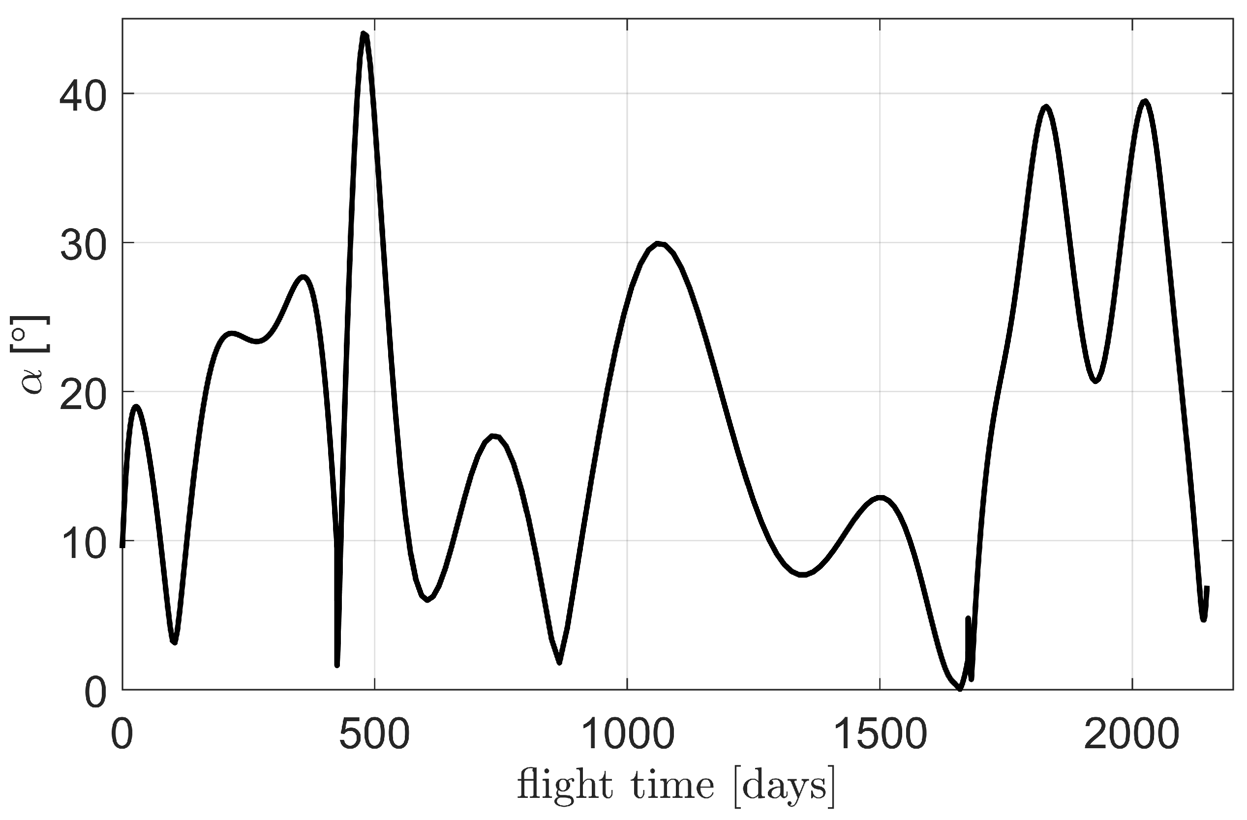
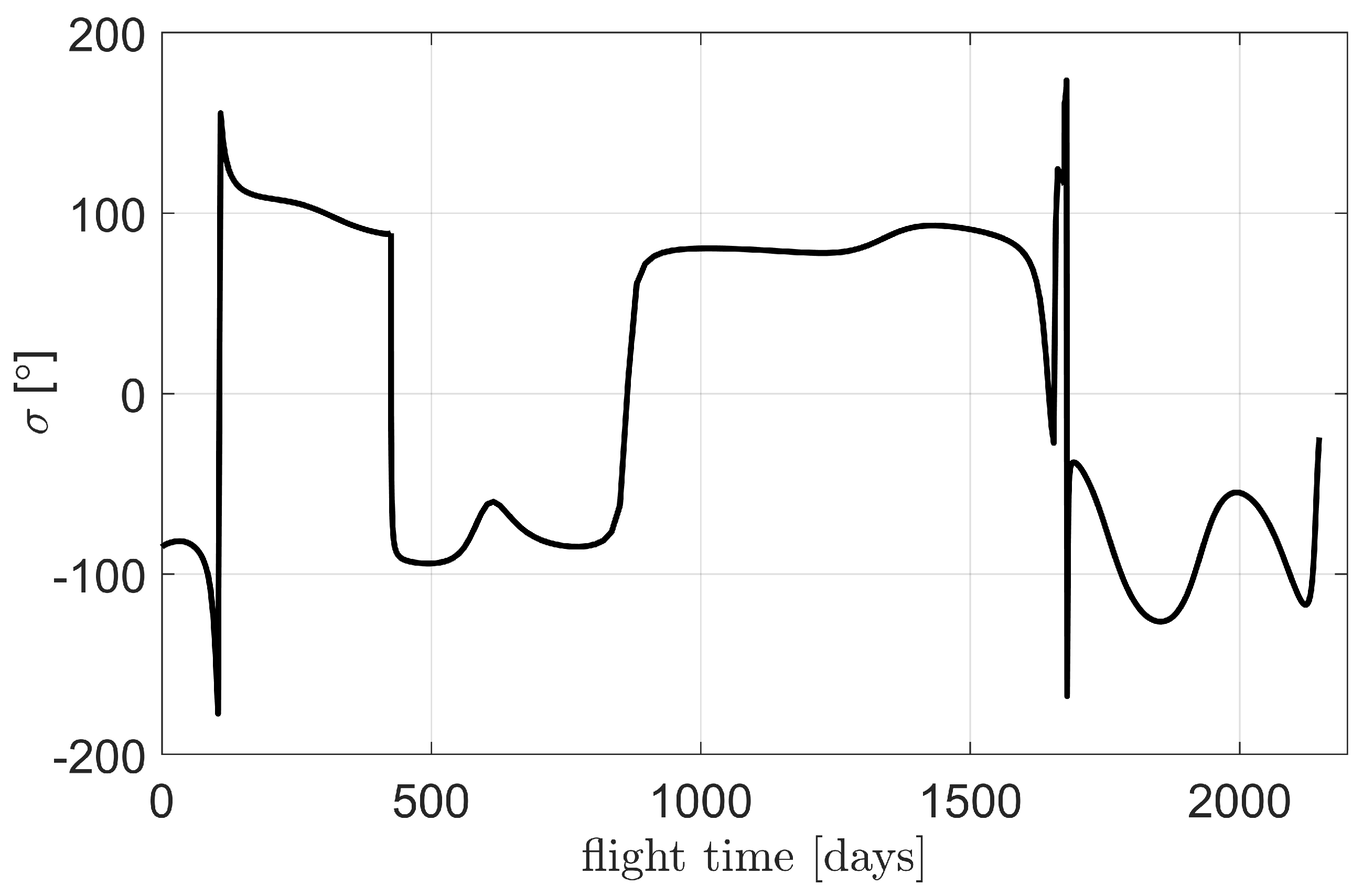
4.1. Mars Gravity Assistance—Solar-System Boundary Exploration

In this simulation example, the E-sail first flies over Mars for exploration, uses Mars for gravity-assist acceleration, and then flies towards the boundary of the solar system. The Modified Julian Day (MJD) for the launch date of the E-sail is 59,096. The simulation results are shown in Figure 4, Figure 5, Figure 6 and Figure 7.

Figure 4 shows the flight trajectories of E-sail’s flyby exploration of Mars, using Mars gravity-assist to increase the heliocentric velocity, and finally reaching the conditions for escaping the solar system. In Figure 4, the diamond represents the position of Mars where the E-sail flew over it. Figure 5 shows the propulsive acceleration curves of the E-sail regarding Mars gravity-assist and solar-system boundary exploration in the orbital coordinate system. Figure 6 and Figure 7 show the time-varying curves of $\alpha$ and $\sigma$ of the E-sail during Mars gravity-assist and solar-system boundary exploration, respectively.

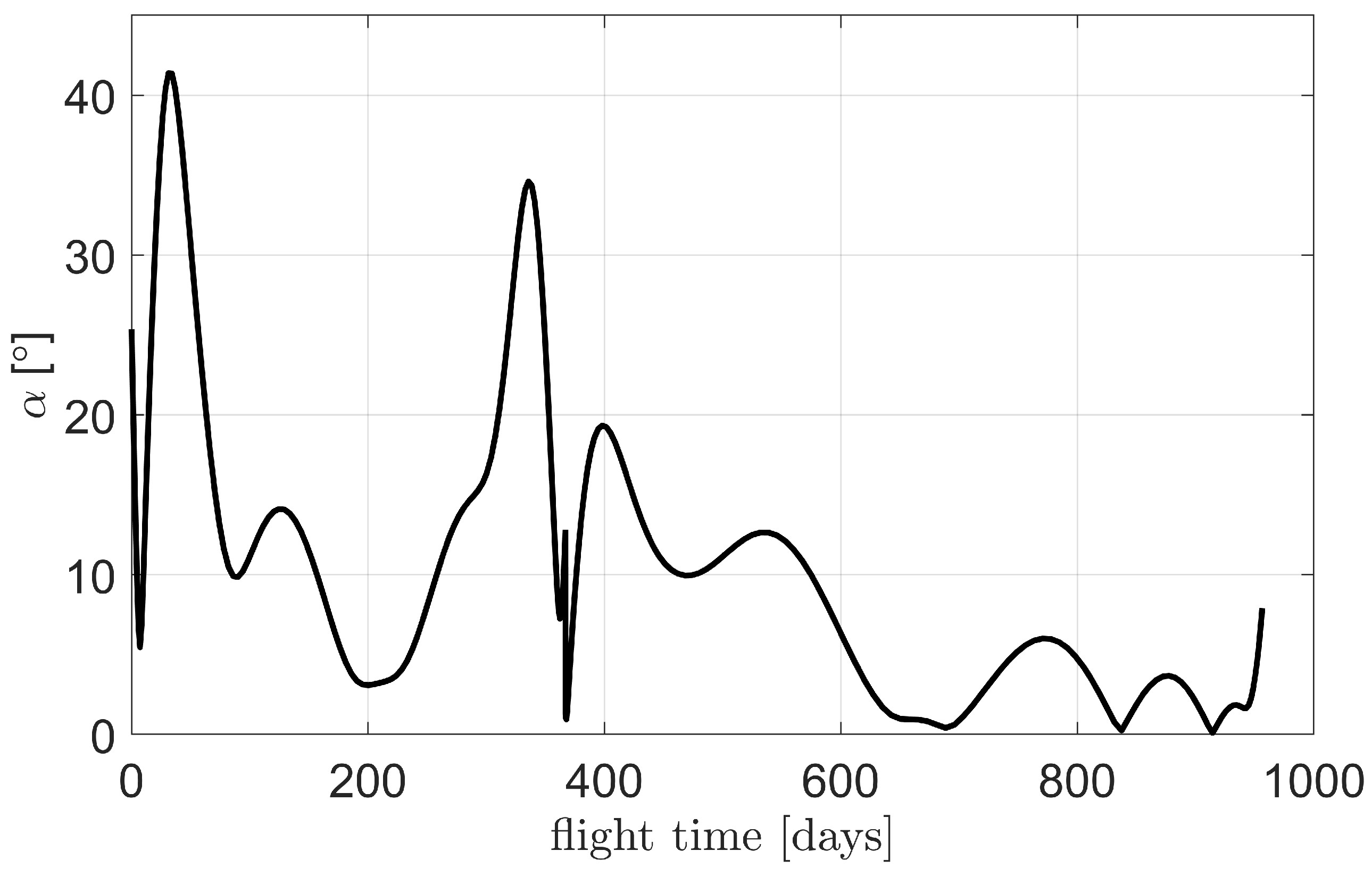
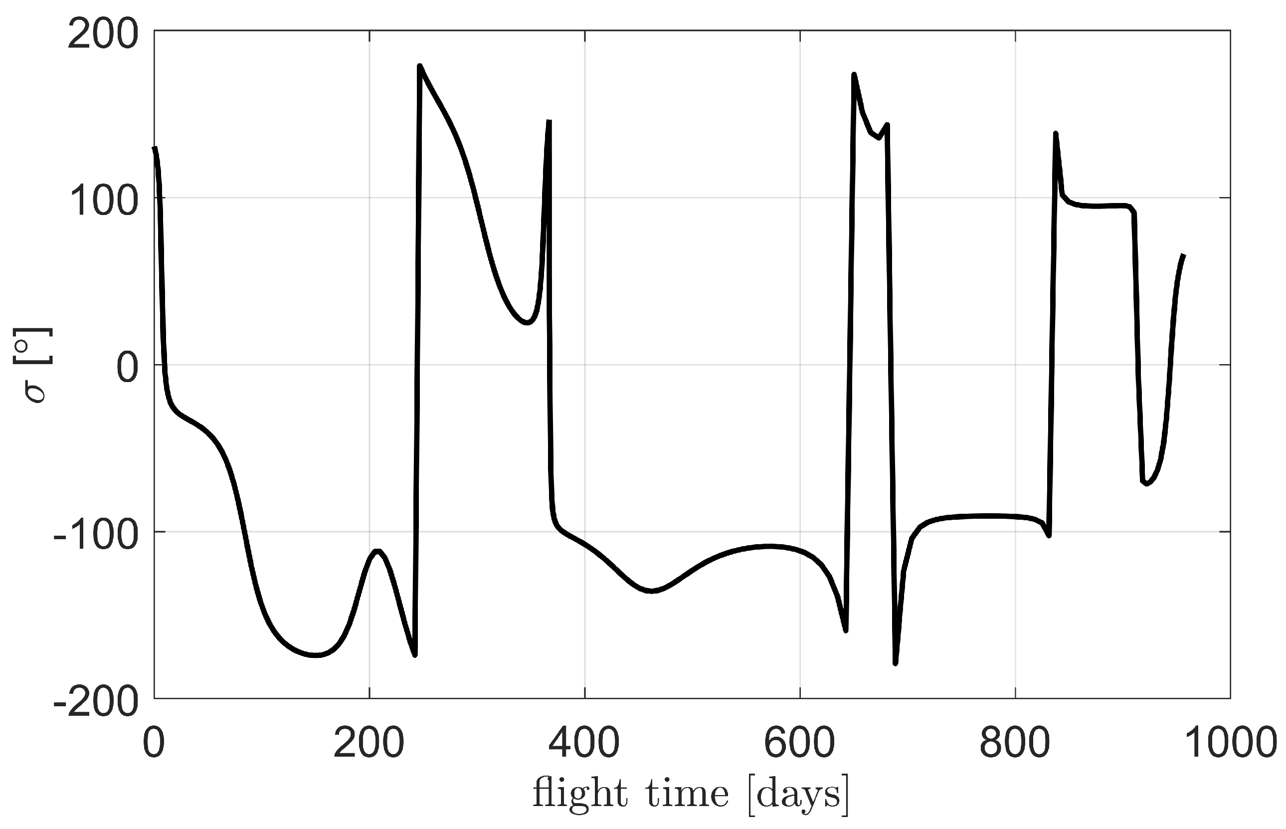
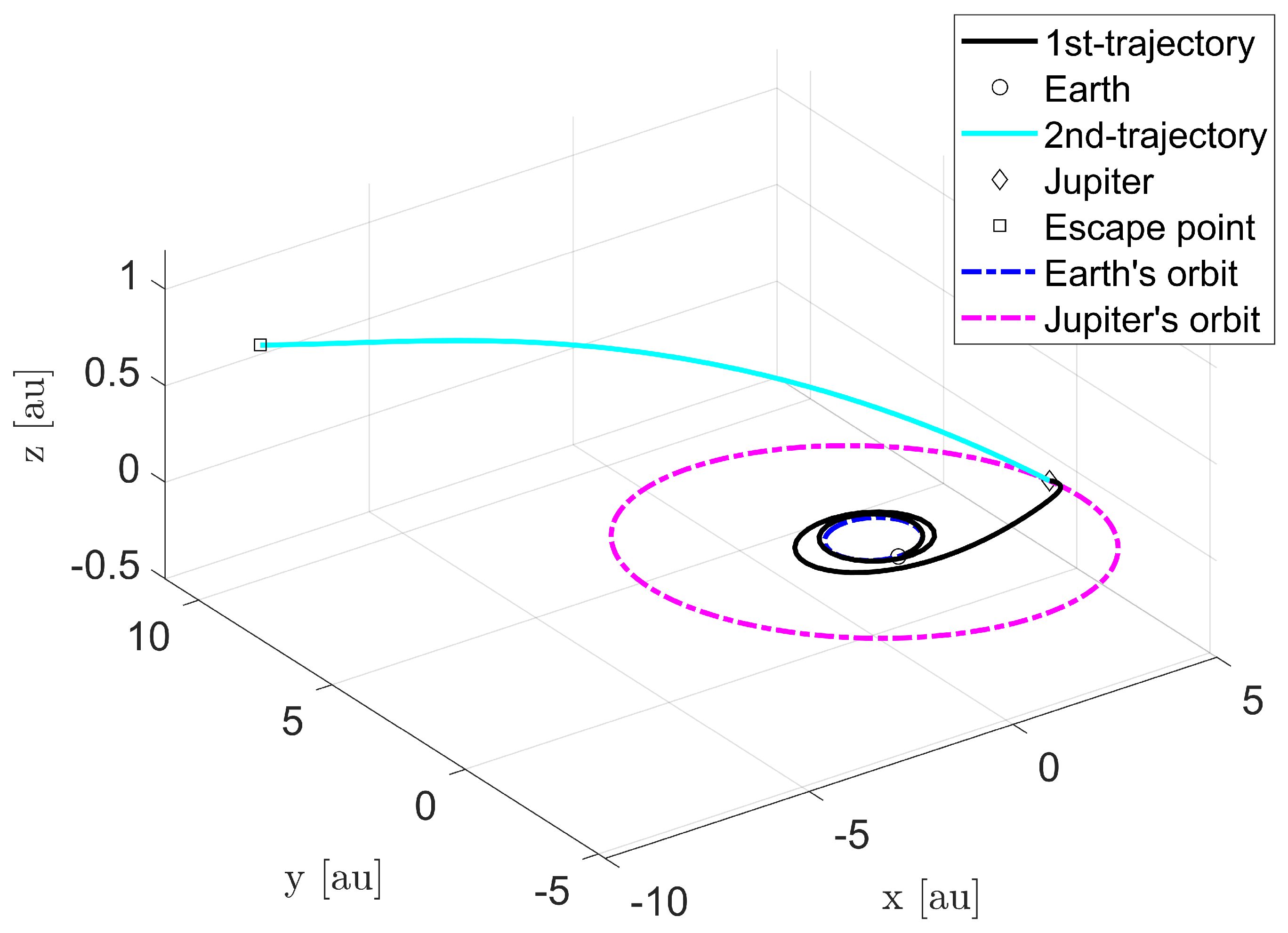
4.2. Jupiter Gravity Assistance—Solar-System Boundary Exploration

In this simulation example, the E-sail first flies over Jupiter for exploration, uses Jupiter for gravity-assist acceleration, and then flies towards the boundary of the solar system. The MJD for the launch date of the E-sail is 62,306. The simulation results are shown in Figure 8, Figure 9, Figure 10 and Figure 11.

Figure 8 shows the flight trajectories of the E-sail’s flyby exploration of Jupiter, using Jupiter gravity-assist for acceleration, and finally reaching the conditions for escaping the solar system. In Figure 8, the diamond represents the position of Jupiter where the E-sail flew over it. Figure 9 shows the propulsive acceleration curves of the E-sail regarding Jupiter gravity-assist and solar-system boundary exploration in the orbital coordinate system. Figure 10 and Figure 11 show the time-varying curves of $\alpha$ and $\sigma$ of the E-sail during Jupiter gravity-assist and solar-system boundary exploration, respectively. Due to the distance between Jupiter and Earth, flying directly to Jupiter for gravitational assistance makes the flight process of the E-sail very difficult. Therefore, the attitude adjustment of E-sail is more complex, and the adjustment range of $\alpha$ is larger.

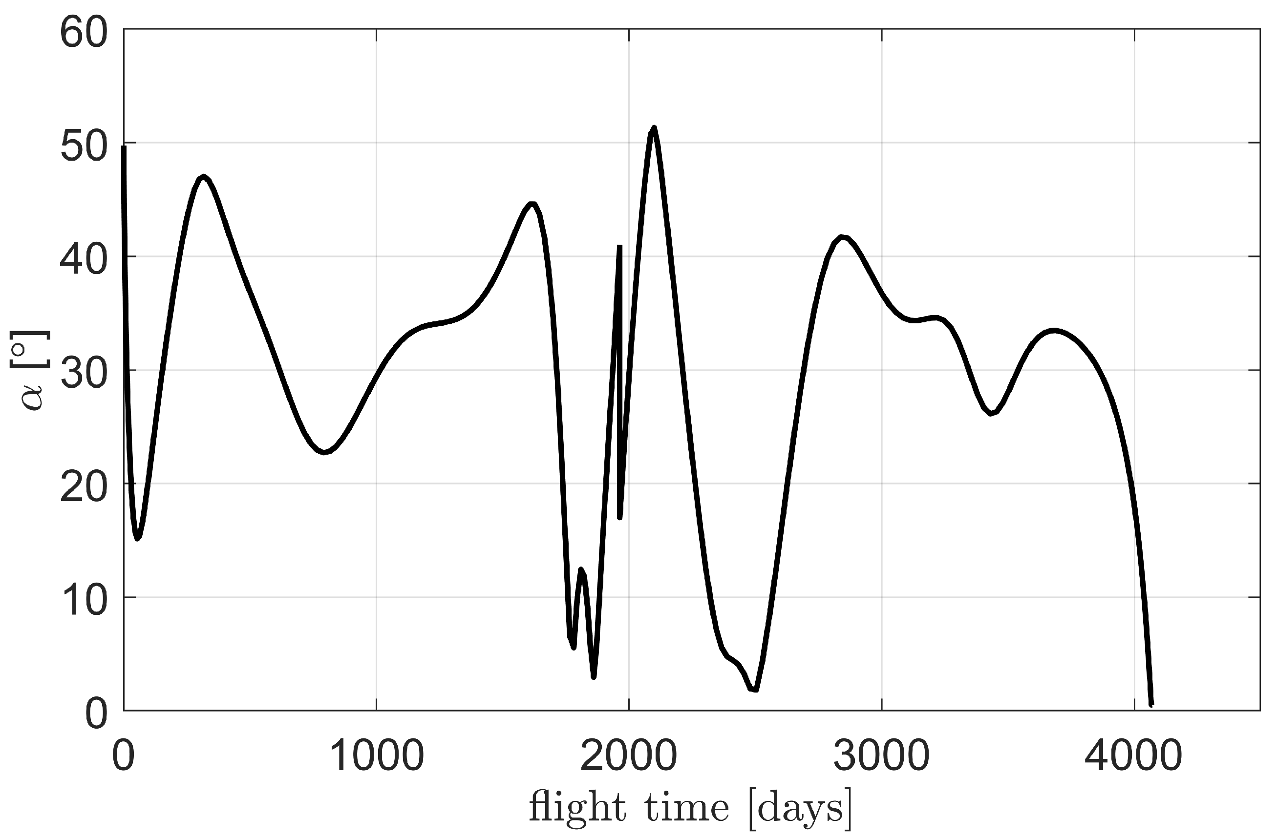
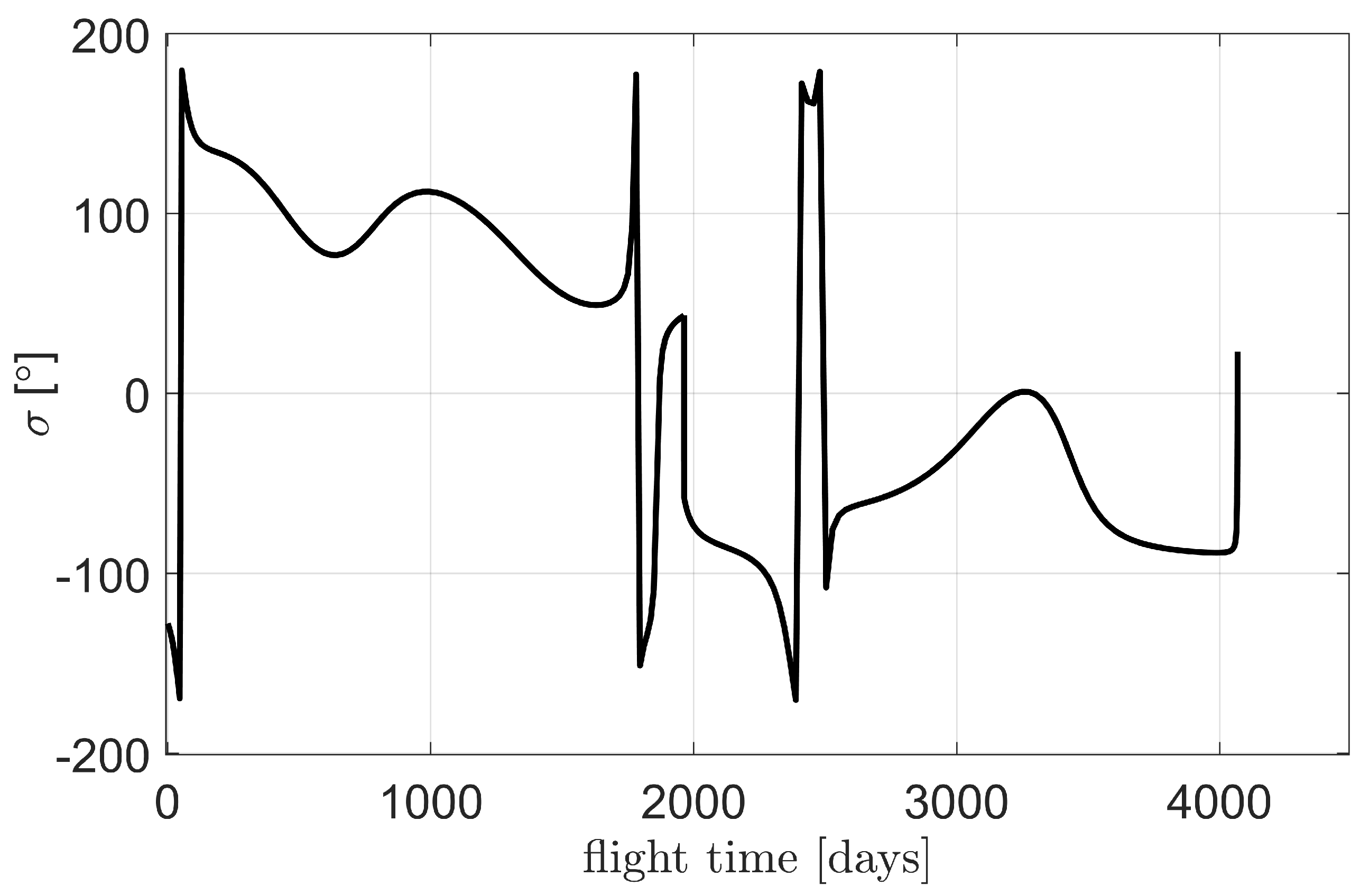
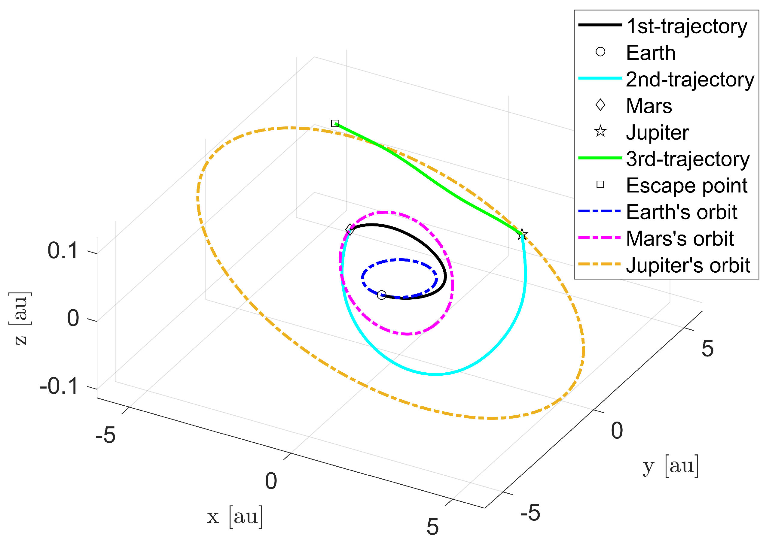
4.3. Mars–Jupiter Gravity Assistance—Solar-System Boundary Exploration

In this simulation example, the E-sail first flies over Mars for exploration and uses Mars for gravity-assist acceleration, then flies over Jupiter for exploration and uses Jupiter for gravity-assist acceleration again, and finally flies towards the boundary of the solar system. The MJD for the launch date of the E-sail is 59,022. The simulation results are shown in Figure 12, Figure 13, Figure 14 and Figure 15.

Figure 12 shows the flight trajectories of the E-sail’s flyby exploration of Mars and Jupiter, using Mars and Jupiter gravity-assist for acceleration, and finally reaching the conditions for escaping the solar system. In Figure 12, the diamond represents the position of Mars where the E-sail flew over Mars, and the star represents the position of Jupiter where the E-sail flew over Jupiter. Figure 13 shows the propulsive acceleration curves of the E-sail regarding Mars and Jupiter gravity-assist and solar-system boundary exploration in the orbital coordinate system. Figure 14 and Figure 15 show the time-varying curves of $\alpha$ and $\sigma$ of the E-sail during Mars and Jupiter gravity-assist and solar-system boundary exploration, respectively.

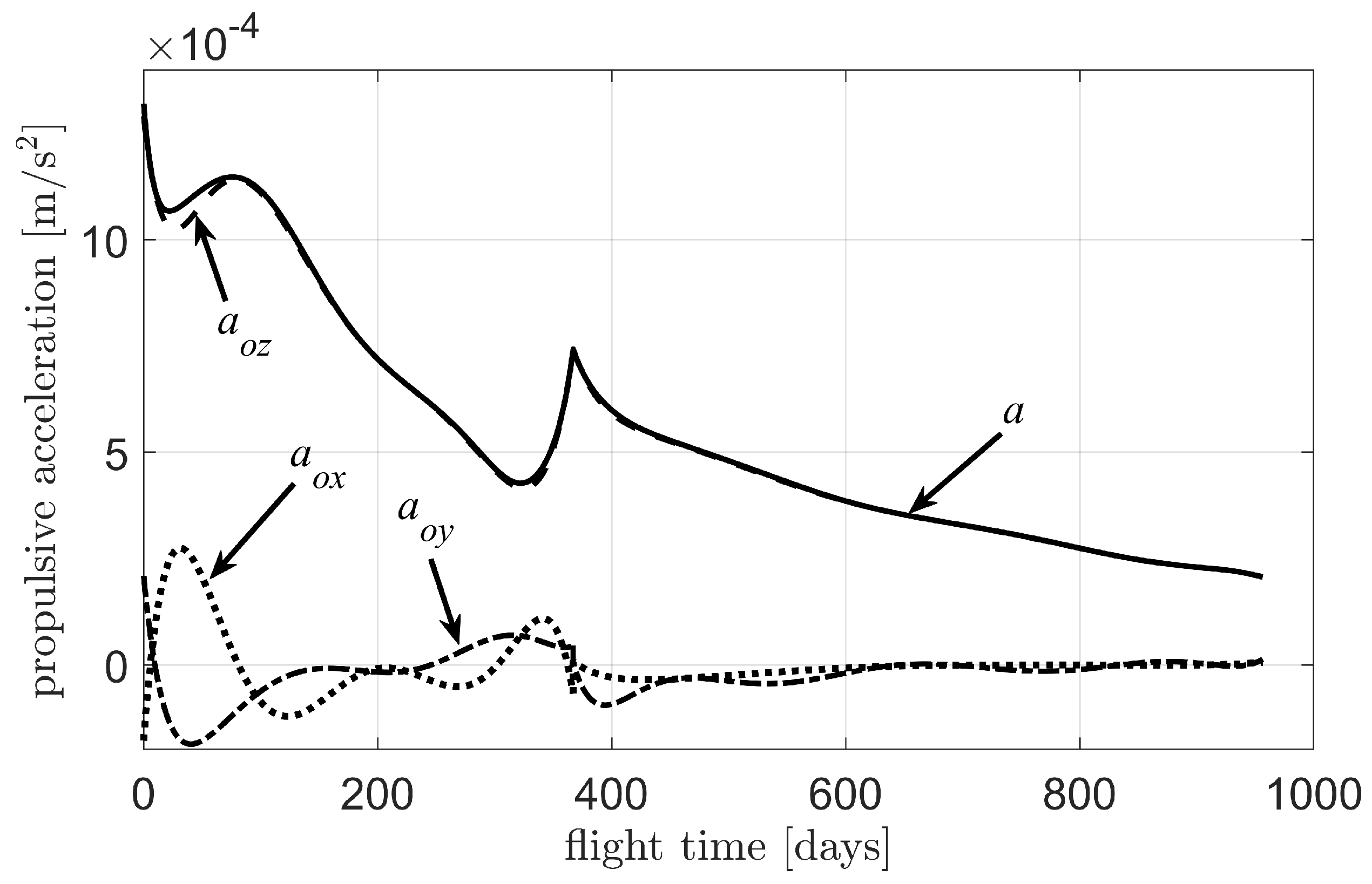
4.4. Simulation Analysis

The computation results of the above three simulation examples are shown in

Table 1. The computation results of the above three simulation examples.

Detection Modes	Detected Targets	Total Flight Time/Years	Computation Time/s
Mars–GA	Mars, SSB	2.62	9.4
Jupiter–GA	Jupiter, SSB	11.15	9.8
Mars–Jupiter–GA	Mars, Jupiter, SSB	5.88	98.8

“GA” stands for “Gravity Assistance”. “SSB” stands for “Solar System Boundary”.

. When using Mars gravity assistance to achieve Mars flyby exploration and obtain the energy to fly to the solar-system boundary, the required flight time is 2.62 years and the computation time is 9.4 s; when using Jupiter’s gravity assistance to achieve Jupiter flyby detection and obtain the energy to fly to the solar-system boundary, the required flight time is 11.15 years and the computation time is 9.8 s; and when utilizing the gravity assistance of Mars and Jupiter to achieve Mars and Jupiter flyby exploration and obtain the energy to fly to the solar-system boundary, the required flight time is 5.88 years and the computation time is 98.8 s. By comparison, it can be seen that when the number of planets involved in flyby detection and gravitational assistance remains constant, the overall computation time remains almost unchanged. However, due to the fact that Jupiter is farther away from Earth than Mars, the flight time for the E-sail to complete the exploration of Jupiter’s flyby has increased; as the number of planets observed with flybys increases, the overall computation time significantly increases due to the more complex flight process. Compared with using Jupiter gravity-assist alone, using multiple gravity assists can shorten the flight time of E-sail by 47.3%, which proves that multiple gravity assists can reduce the overall flight time. From the simulation analysis above, it can be seen that the method proposed in this paper can quickly obtain flight trajectories for different detection targets and flight situations. The efficiency of the algorithm proposed in this paper is of great significance for the rapid analysis of initial missions.

5. Conclusions

This paper proposes an optimization algorithm for multi-target exploration trajectories of the E-sail, which considers planetary flyby exploration, solar-system boundary exploration, and gravity-assisted maneuvering. Through simulation analysis, it is proven that when using a planet for gravitational assistance to achieve planetary flyby detection and solar-system boundary detection, the method proposed in this paper can obtain feasible solutions within 10 s; when using multiple forms of gravitational assistance, feasible solutions can also be obtained within 100 s. The method proposed in this article has good performance in quickly solving complex problems such as multi-planet detection, solar-system boundary detection, and gravity-assist maneuvering. This also proves that the method proposed in this article is of great significance for the rapid initial analysis of complex deep-space exploration missions.

References

1. Qi, N.; Fan, Z.; Huo, M.; Du, D.; Zhao, C. Fast trajectory generation and asteroid sequence selection in multispacecraft for multiasteroid exploration. IEEE Trans. Cybern. 2022, 52, 6071–6082. [Google Scholar] [CrossRef] [PubMed]
2. Simone, C.; Matteo, C.; Paolo, G.; Stefano, S. Proprioceptive swarms for celestial body exploration. Acta Astronaut. 2024, 223, 159–174. [Google Scholar]
3. Bassetto, M.; Niccolai, L.; Quarta, A.; Mengali, G. A comprehensive review of Electric Solar Wind Sail concept and its applications. Prog. Aerosp. Sci. 2022, 128, 100768. [Google Scholar] [CrossRef]
4. Palos, M.F.; Janhunen, P.; Toivanen, P.; Tajmar, M.; Iakubivskyi, I.; Micciani, A.; Orsini, N.; Kütt, J.; Rohtsalu, A.; Dalbins, J.; et al. Electric Sail Mission Expeditor, ESME: Software Architecture and Initial ESTCube Lunar Cubesat E-Sail Experiment Design. Aerospace 2023, 10, 694. [Google Scholar] [CrossRef]
5. Slavinskis, A.; Palos, M.F.; Dalbins, J.; Janhunen, P.; Tajmar, M.; Ivchenko, N.; Rohtsalu, A.; Micciani, A.; Orsini, N.; Moor, K.M.; et al. Electric Sail Test Cube–Lunar Nanospacecraft, ESTCube-LuNa: Solar Wind Propulsion Demonstration Mission Concept. Aerospace 2024, 11, 230. [Google Scholar] [CrossRef]
6. Niccolai, L. Optimal deep-space heliocentric transfers with an electric sail and an electric thruster. Adv. Space Res. 2024, 73, 85–94. [Google Scholar] [CrossRef]
7. Niccolai, L.; Anderlini, A.; Mengali, G.; Quarta, A. Impact of solar wind fluctuations on Electric Sail mission design. Aerosp. Sci. Technol. 2018, 82–83, 38–45. [Google Scholar] [CrossRef]
8. Caruso, A.; Niccolai, L.; Mengali, G.; Quarta, A. Electric sail trajectory correction in presence of environmental uncertainties. Aerosp. Sci. Technol. 2019, 94, 105395. [Google Scholar] [CrossRef]
9. Quarta, A.A. Impact of Pitch Angle Limitation on E-Sail Interplanetary Transfers. Aerospace 2024, 11, 729. [Google Scholar] [CrossRef]
10. Quarta, A.A.; Mengali, G. Electric Sail Mission Analysis for Outer Solar System Exploration. J. Guid. Control Dyn. 2010, 33, 740–755. [Google Scholar] [CrossRef]
11. Niccolai, L.; Quarta, A.; Mengali, G. Exploration of Asteroids and Comets with Innovative Propulsion Systems. In Handbook of Space Resources; Badescu, V., Zacny, K., Bar-Cohen, Y., Eds.; Springer: Cham, Switzerland, 2003; pp. 841–869. [Google Scholar]
12. Niccolai, L.; Bassetto, M.; Quarta, A.A.; Mengali, G. Optimal Earth Gravity-Assist Maneuvers with an Electric Solar Wind Sail. Aerospace 2022, 9, 717. [Google Scholar] [CrossRef]
13. Rao, A.V.; Benson, D.A.; Darby, C.; Patterson, M.A.; Francolin, C.; Sanders, I.; Huntington, G.T. Algorithm 902: GPOPS, a matlab software for solving multiple-phase optimal control problems using the Gauss pseudospectral method. ACM Trans. Math. Softw. 2010, 37, 22. [Google Scholar] [CrossRef]
14. Tang, G.; Jiang, F.; Li, J. Fuel-optimal low-thrust trajectory optimization using indirect method and successive convex programming. IEEE Trans. Aerosp. Electron. Syst. 2018, 54, 2053–2066. [Google Scholar] [CrossRef]
15. Oshima, K. Regularized direct method for low-thrust trajectory optimization: Minimum-fuel transfer between cislunar periodic orbits. Adv. Space Res. 2023, 72, 2051–2063. [Google Scholar] [CrossRef]
16. Sidhoum, Y.; Oguri, K. On the Performance of different smoothing methods for indirect low-thrust trajectory optimization. J. Astronaut. Sci. 2023, 70, 51. [Google Scholar] [CrossRef]
17. Quarta, A.; Mengali, G.; Bassetto, M.; Niccolai, L. Optimal Circle-to-Ellipse Orbit Transfer for Sun-Facing E-Sail. Aerospace 2022, 9, 671. [Google Scholar] [CrossRef]
18. Xie, C.; Zhang, G.; Zhang, Y. Shaping approximation for low-thrust trajectories with large out-of-plane motion. J. Guid. Control. Dyn. 2016, 39, 2776–2785. [Google Scholar] [CrossRef]
19. Zeng, K.; Geng, Y.; Wu, B. Shape-based analytic safe trajectory design for spacecraft equipped with low-thrust engines. Aerosp. Sci. Technol. 2017, 62, 87–97. [Google Scholar] [CrossRef]
20. Fan, Z.; Huo, M.; Qi, N.; Zhao, C.; Yu, Z.; Lin, T. Initial Design of Low-Thrust Trajectories Based on the Bezier Curve-based Shaping Approach. Proc. Inst. Mech. Eng. Part G J. Aerosp. Eng. 2020, 234, 1825–1835. [Google Scholar] [CrossRef]
21. Gondelach, D.J.; Noomen, R. Hodographic-shaping method for low-thrust interplanetary trajectory design. J. Apacecraft Rocket. 2015, 52, 728–738. [Google Scholar] [CrossRef]
22. Fan, Z.; Huo, M.; Quarta, A.A.; Mengali, G.; Qi, N. Improved Monte Carlo Tree Search-based approach to low-thrust multiple gravity-assist trajectory design. Aerosp. Sci. Technol. 2022, 130, 107946. [Google Scholar] [CrossRef]
23. Huo, M.; Fan, Z.; Qi, J.; Qi, N.; Zhu, D. Fast analysis of multi-asteroid exploration mission using multiple electric sails. J. Guid. Control. Dyn. 2023, 46, 1015–1022. [Google Scholar] [CrossRef]
24. Wall, B.J.; Conway, B.A. Shape-Based approach to low-thrust rendezvous trajectory design. J. Guid. Control Dyn. 2009, 32, 95–101. [Google Scholar] [CrossRef]
25. Shang, H.; Cui, P.; Qiao, D. A shape-based design approach to interplanetary low-thrust transfer trajectory. J. Astronaut. 2010, 31, 1569–1574. [Google Scholar]
26. Novak, D.M.; Vasile, M. Improved shaping approach to the preliminary design of low-thrust trajectories. J. Guid. Control Dyn. 2011, 34, 128–147. [Google Scholar] [CrossRef]
27. Huo, M.; Zhang, G.; Qi, N.; Liu, Y.; Shi, X. Initial trajectory design of electric solar wind sail based on finite Fourier series shape-based method. IEEE Trans. Aerosp. Electron. Syst. 2019, 55, 3674–3683. [Google Scholar] [CrossRef]
28. Huo, M.; Mengali, G.; Quarta, A.A.; Qi, N. Electric sail trajectory design with bezier curve-based shaping approach. Aerosp. Sci. Technol. 2019, 88, 126–135. [Google Scholar] [CrossRef]
29. Petropoulos, A.E.; Longuski, J.M. Shape-based algorithm for automated design of low-thrust, gravity-assist trajectories. J. Spacecr. Rocket. 2004, 41, 787–796. [Google Scholar] [CrossRef]
30. Abdelkhalik, O.; Taheri, E. Approximate on-off low-thrust space trajectories using Fourier series. J. Spacecr. Rocket. 2012, 49, 962–965. [Google Scholar] [CrossRef]
31. Taheri, E.; Abdelkhalik, O. Fast initial trajectory design for low-thrust restricted-three-body problems. J. Guid. Control Dyn. 2015, 38, 2146–2160. [Google Scholar] [CrossRef]
32. Taheri, E.; Abdelkhalik, O. Initial three-dimensional low-thrust trajectory design. Adv. Space Res. 2016, 57, 889–903. [Google Scholar] [CrossRef]
33. Bassetto, M.; Quarta, A.; Mengali, G. Locally-optimal electric sail transfer. Proc. Inst. Mech. Eng. Part G-J. Aerosp. Eng. 2019, 233, 166–179. [Google Scholar] [CrossRef]
Figure 1. Coordinate systems [27].
Aerospace 12 00196 g001
Figure 2. Propulsive acceleration’s characteristic angles [27].
Aerospace 12 00196 g002
Figure 3. Gravity-assist process.
Aerospace 12 00196 g003
Figure 4. Mars gravity-assist and solar-system boundary exploration transfer trajectories.
Aerospace 12 00196 g004
Figure 5. Time variation of the E-sail propulsive acceleration components in the orbital coordinate system (Mars–solar-system boundary).
Aerospace 12 00196 g005
Figure 6. Time variation of attitude angle α (Mars–solar-system boundary).
Aerospace 12 00196 g006
Figure 7. Time variation of attitude angle σ (Mars–solar-system boundary).
Aerospace 12 00196 g007
Figure 8. Jupiter gravity-assist and solar-system boundary exploration transfer trajectories.
Aerospace 12 00196 g008
Figure 9. Time variation of the E-sail propulsive acceleration components in the orbital coordinate system (Jupiter–solar-system boundary).
Aerospace 12 00196 g009
Figure 10. Time variation of attitude angle α (Jupiter–solar-system boundary).
Aerospace 12 00196 g010
Figure 11. Time variation of attitude angle σ (Jupiter–solar-system boundary).
Aerospace 12 00196 g011
Figure 12. Mars and Jupiter gravity-assist and solar-system boundary exploration transfer trajectories.
Aerospace 12 00196 g012
Figure 13. Time variation of the E-sail propulsive acceleration components in the orbital coordinate system (Mars–Jupiter–solar-system boundary).
Aerospace 12 00196 g013
Figure 14. Time variation of attitude angle α (Mars–Jupiter–solar-system boundary).
Aerospace 12 00196 g014
Figure 15. Time variation of attitude angle σ (Mars–Jupiter–solar-system boundary).
Aerospace 12 00196 g015